| Issue |
A&A
Volume 620, December 2018
|
|
|---|---|---|
| Article Number | A28 | |
| Number of page(s) | 16 | |
| Section | Catalogs and data | |
| DOI | https://doi.org/10.1051/0004-6361/201833588 | |
| Published online | 26 November 2018 | |
Deep XMM-Newton observations of the northern disc of M 31
I. Source catalogue⋆,⋆⋆
1
Dr. Karl Remeis Observatory and ECAP, Universität Erlangen-Nürnberg, Sternwartstr. 7, 96049 Bamberg, Germany
e-mail: manami.sasaki@fau.de
2
Max-Planck-Institut für extraterrestrische Physik, Giessenbachstraße, 85748 Garching, Germany
3
Department of Astronomy, San Diego State University, San Diego, CA, 92182 USA
4
Institute of Space Sciences (IEEC-CSIC), Campus UAB, Carrer de Can Magrans, s/n, 08193 Barcelona, Spain
5
Institut für Astronomie und Astrophysik, Universität Tübingen, Sand 1, 72076 Tübingen, Germany
6
Astronomy Department, University of Washington, Box 351580
Seattle, WA, 98195 USA
7
Harvard-Smithsonian Center for Astrophysics, 60 Garden Street, Cambridge, MA, 02138 USA
8
Department of Astrophysics, Astronomy & Mechanics, Faculty of Physics, University of Athens, 15783 Athens, Greece
9
IAASARS, National Observatory of Athens, Vas. Pavlou & I. Metaxa, 15236 Penteli, Greece
10
American Community Schools of Athens, 129 Aghias Paraskevis Ave. & Kazantzaki Street, Halandri, 15234 Athens, Greece
11
Sternberg Astronomical Institute, Moscow State University, Universitetskii pr. 13, 119992 Moscow, Russia
12
Astro Space Center of Lebedev Physical Institute, Profsoyuznaya St. 84/32, 117997 Moscow, Russia
13
Zentrum fürAstronomie und Astrophysik, Technische Universität Berlin, Hardenbergstrasse 36, 10623 Berlin, Germany
14
Department of Mathematics, University of Évora, R. Romão Ramalho 59, 7000 Évora, Portugal
15
Western Sydney University, Locked Bag 1791, Penrith, NSW, 2751 Australia
16
CSIRO Astronomy and Space Science, PO Box 1130
Bentley Delivery Centre, WA, 6983 Australia
17
School of Cosmic Physics, Dublin Institute for Advanced Studies, 31 Fitzwillam Place, Dublin 2, Ireland
18
Space Telescope Science Institute, 3700 San Martin Drive, Baltimore, MD, 21218 USA
Received:
7
June
2018
Accepted:
19
September
2018
Context. We carried out new observations of two fields in the star-forming northern ring of M 31 with XMM-Newton with each one of them consisting of two exposures of about 100 ks each. A previous XMM-Newton survey of the entire M 31 galaxy revealed extended diffuse X-ray emission in these regions.
Aims. We study the population of X-ray sources in the northern disc of M 31 by compiling a complete list of X-ray sources down to a sensitivity limit of ∼7 × 1034 erg s−1 (0.5–2.0 keV) and improve the identification of the X-ray sources. The major objective of the observing programme was the study of the hot phase of the interstellar medium (ISM) in M 31. The analysis of the diffuse emission and the study of the ISM is presented in a separate paper.
Methods. We analysed the spectral properties of all detected sources using hardness ratios and spectra if the statistics were high enough. We also checked for variability. In order to classify the sources detected in the new deep XMM-Newton observations, we cross-correlated the source list with the source catalogue of a new survey of the northern disc of M 31 carried out with the Chandra X-ray Observatory and the Hubble Space Telescope (Panchromatic Hubble Andromeda Treasury, PHAT) as well as with other existing catalogues.
Results. We detected a total of 389 sources in the two fields of the northern disc of M 31 observed with XMM-Newton. We identified 43 foreground stars and candidates and 50 background sources. Based on a comparison with the results of the Chandra/PHAT survey, we classify 24 hard X-ray sources as new candidates for X-ray binaries. In total, we identified 34 X-ray binaries and candidates and 18 supernova remnants (SNRs) and candidates. We studied the spectral properties of the four brightest SNRs and confirmed five new X-ray SNRs. Three of the four SNRs, for which a spectral analysis was performed, show emission mainly below 2 keV, which is consistent with shocked ISM. The spectra of two of them also require an additional component with a higher temperature. The SNR [SPH11] 1535 has a harder spectrum and might suggest that there is a pulsar-wind nebula inside the SNR. For all SNRs in the observed fields, we measured the X-ray flux or calculated upper limits. We also carried out short-term and long-term variability studies of the X-ray sources and found five new sources showing clear variability. In addition, we studied the spectral properties of the transient source SWIFT J004420.1+413702, which shows significant variation in flux over a period of seven months (June 2015 to January 2016) and associated change in absorption. Based on the likely optical counterpart detected in the Chandra/PHAT survey, the source is classified as a low-mass X-ray binary.
Key words: galaxies: individual: M 31 / X-rays: binaries / X-rays: ISM / ISM: supernova remnants
Based on observations obtained with XMM-Newton, an ESA science mission with instruments and contributions directly funded by ESA Member States and NASA.
Tables A.1–A.6 are only available at the CDS via anonymous ftp to cdsarc.u-strasbg.fr (130.79.128.5) or via http://cdsarc.u-strasbg.fr/viz-bin/qcat?J/A+A/620/A28
© ESO 2018
1. Introduction
The Andromeda galaxy (M 31) is the largest galaxy in the Local Group and the nearest spiral galaxy to the Milky Way, located at a distance of 783 kpc (Conn et al. 2016). With a similar mass and metallicity to our Galaxy, it is also the closest example of the type of galaxy that dominates redshift surveys. This archetypal spiral galaxy thus provides a unique opportunity to study and understand the nature and the evolution of a galaxy similar to our own.
The star-formation history in M 31 has been studied in detail in observations with both the Hubble Space Telescope (HST) and large ground-based telescopes (e.g., the Local Group Survey, LGS, Massey et al. 2002, 2006). Deep HST photometry has shown that the mean age of the disc of M 31 is 6 − 8 Gyr (Brown et al. 2006). Williams (2003) measured a mean star-formation rate of about 1 M⊙ yr−1 in the full disc of M 31 and produced maps of star-formation rate in different age ranges. In addition, the northern disc was observed with the HST over a period of 4 years in the Panchromatic Hubble Andromeda Treasury (PHAT) survey (Dalcanton et al. 2012). Each field was observed with the Advanced Camera for Surveys (ACS) and the Wide Field Camera 3 (WFC3) yielding photometry of over 100 million stars in M 31 from the near-infrared (NIR) to the ultraviolet (UV) (Williams et al. 2014b). Based on these data the star-formation history has been measured on a scale of a few hundred parsecs (Williams et al. 2017).
At longer wavelengths, Gordon et al. (2006), using data taken with the Spitzer Space Telescope, showed that M 31 has spiral-arm structures merged with a prominent star-forming ring at a radius of ∼10 kpc. The newest images of the Herschel Space Observatory show a radial gradient in the gas-to-dust ratio and indicate that there are two distinct regions in M 31 with different dust properties inside and outside R ≈ 3.1 kpc (Smith et al. 2012; Fritz et al. 2012). In addition to the well-known dust ring at a radius of ∼10 kpc (Brinks & Shane 1984; Dame et al. 1993) with enhanced star formation, Block et al. (2006) found a dust ring with a radius of 1–1.5 kpc, which had apparently been created in an encounter with a companion galaxy, most likely M 32.
The first observations of individual sources in M 31 in X-rays were performed with the Einstein Observatory in the energy band of 0.2–4.5 keV and yielded the first catalogues of X-ray sources in the field of M 31 (van Speybroeck et al. 1979; Trinchieri & Fabbiano 1991). In the 1990s, M 31 was observed with the Röntgen Satellite ROSAT in the 0.1–2.4 keV band. A total of 560 sources were confirmed in the field of M 31 (Supper et al. 1997, 2001). More recent observations with the next-generation X-ray satellites Chandra X-ray Observatory and X-ray Multi-Mirror Mission (XMM-Newton) have provided a comprehensive list of X-ray sources and allowed the study of individual objects (e.g. Osborne et al. 2001; Kong et al. 2002b; Kaaret 2002; Williams et al. 2004, 2006; Pietsch et al. 2005; Trudolyubov et al. 2005; Stiele et al. 2008; Barnard et al. 2008; Vulic et al. 2016) in selected regions as well as in a survey of the entire M 31 galaxy performed with XMM-Newton between June 2006 and February 2008. The catalogue of the first XMM-Newton survey of M 31 with 856 sources was published by Pietsch et al. (2005; hereafter PFH05) and an updated XMM-Newton catalogue with 1948 sources by Stiele et al. (2011), hereafter SPH11).
We performed new deep observations of the northern star-forming disc of M 31 with XMM-Newton in order to study the morphology and properties of the hot interstellar medium (ISM) and to study the star-formation history of M 31 by achieving a much lower flux limit than before and thus obtaining a more complete sample of X-ray sources in M 31. The first results relating to transient sources were reported by Henze et al. (2015a, b, 2016a, b, c). In this paper, we present the point source catalogue of the new deep XMM-Newton observations of the northern disc of M 31. The study of the ISM using the new XMM-Newton data is presented in a dedicated paper by Kavanagh et al. (in prep.).
2. Observations and data analysis
We observed two fields in the northern disc of M 31 in a large programme (LP) of XMM-Newton (PI: M. Sasaki). The data were taken with the European Photon Imaging Cameras (EPICs, Strüder et al. 2001; Turner et al. 2001) in full-frame mode using the thin filter for the pn camera (EPIC-pn) and the medium filter for the two MOS cameras (EPIC-MOS1/2) in order to minimise the contamination from background and maximise the sensitivity for soft diffuse emission. Each of the two fields was observed twice. The observation IDs and effective exposure times are given in Table 1. We had requested a total exposure of 200 ks for each field split into two observations separated by 6 months to study the variability of the sources. While the first three observations (ObsIDs 0763120101, 0763120301, and 0763120401) were carried out with exposure times of ∼90–100 ks, observation 0763120201 was affected by high background flares. The data were analysed using the XMM-Newton Science Analysis System (SAS) version 15.0.0. Data processing and analysis were performed in the same manner as in Sturm et al. (2013).
List of XMM-Newton LP observations of the northern disc of M 31.
2.1. Source detection
In order to perform source detection, images of each observation were created for each one of the three cameras in the energy bands of B1 = 0.2–0.5 keV, B2 = 0.5–1.0 keV, B3 = 1.0–2.0 keV, B4 = 2.0–4.5 keV, and B5 = 4.5–12.0 keV. Source detection was performed simultaneously on all 15 images for each observation. Details of the source detection routine and possible uncertainties can be found in Sturm et al. (2013). We thus obtained one final source list for each observation. This source list includes information such as the source position, detection likelihood, count rate, and hardness ratios (see Sect. 3.1) for each detection.
2.2. Astrometry correction
In order to improve the astrometry of the XMM-Newton sources, we cross-correlated the source list obtained from the source detection routine with the USNO-B1.0 catalogue (Monet et al. 2003) in the optical and the 2MASS catalogue (Skrutskie et al. 2006) in the NIR for each observation. The USNO-B1.0 catalogue also contains proper motion information for the stars, which was taken into account when comparing the X-ray position with the optical position. For each cross-correlation result, the optical/NIR position at the epoch of the XMM-Newton observation was plotted on optical I, V, U images of the Local Group Survey (LGS, Massey et al. 2002, 2006) together with the XMM-Newton positions and verified by eye. In addition, the list was cross-correlated with the XMM-Newton catalogue of SPH11, in which the X-ray sources had been classified. Of particular interest for the astrometric correction are the foreground stars (fgStars) and the background active galactic nuclei (AGNs). Only firm correlations between the optical/NIR and the X-ray positions of sources which had been identified as foreground stars or as AGNs were used to calculate the weighted mean of the linear offset between the optical/NIR and X-ray positions for RA and Dec separately, using the inverse of the positional error of the X-ray detections as weights. The weighted means of the offsets in RA or Dec for the four observations were in the range of 0.01″–2.13″. These weighted means were then used to correct the attitude information for each observation (see Table 1). The entire source detection routine and the following cross-correlation of the source lists with the catalogues were carried out once more using the astrometrically aligned data. The linear offset to the optical and NIR positions for X-ray sources identified as foreground stars or AGNs was reduced to < 0.5″. After the correction, the offsets between coordinates had a mean dispersion of ∼1.2″, which is comparable to the mean positional error of the detections (1.25″).
2.3. Artefacts
The raw source list produced by the standard detection algorithm includes some false detections, which have to be removed. False detections arise for a number of reasons: out-of-time (OOT) events, chip gaps, edges of the field of view (FOV), or wings of the point-spread function (PSF) of brighter sources. Therefore, not all the significant detections resulting from the source detection routine are real astrophysical sources. In addition, part of a diffuse emission in a region crowded with sources can also be listed as a source.
Out-of-time events are caused when bright sources are observed with EPIC-pn. In this case many photons are registered while the CCD is read out, resulting in incorrect values for the position along the read-out (RAWY) and thus causing the emission spread over the entire column. Detections of OOT events as sources can be identified and removed by comparing the EPIC-pn image to the EPIC-MOS1/2 images of the same observation.
In order to remove the false detections, we inspected all images one by one and verified the detections in our source list. Also, the detections on different cameras and different observations were compared with each other. False detections caused by OOT events, chip gaps, FOV edges, and wings of the PSF were marked as such and removed from the final source list. Sources detected inside a crowded region with supernova remnants (SNRs) or H II regions were marked as “diffuse”. Such a detection was kept in the source list if it could be clearly identified with a source after the comparison with other catalogues and data (see Sect. 2.5). The number of detected sources in the four observations was originally 187, 125, 206, and 153, from which 9, 2, 10, and 9 sources were removed, respectively (sorted by ObsID).
2.4. Final source list
Once the artefacts were removed, the four detection lists of the four new XMM-Newton LP observations were combined into one final source list with 389 sources. Since each of the two positions in the northern disc of M 31 was observed twice, most of the sources were detected in two observations. In overlapping regions, there are also sources which are detected three or four times. In these cases of multiple detections, the detection with the highest detection likelihood, and thus the most statistically significant detection, was selected for the final source list. Typically, this also corresponds to the detection with the best positional accuracy. The final source list can be found in Table A.1. This table also includes the classification of the sources, either from Sasaki et al. (2012, see Sect. 2.5) or newly defined in this work. Candidates of a source class are given in <> brackets. A mosaic image of the four observations is shown in Fig. 1. More SNRs and X-ray binaries (XRBs) are found closer to the galactic centre than in the other parts of the galactic disc (see Fig. 1, left). In addition, SNRs are likely located in the ring of M 31. Supersoft sources are found closer to the nuclear region.
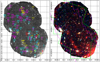 |
Fig. 1. Left: exposure-corrected mosaic image in the energy band 0.2–1.0 keV. Marked sources are: cyan (XRBs and candidates), yellow (SNRs and candidates), red (SSSs and candidates). XRBs and candidates, for which a spectral analysis was performed, are additionally marked with a circle (see Sect. 3.2). Background sources with fitted spectra are marked with magenta circles. Right: exposure-corrected mosaic images of the XMM-Newton LP observations of the northern disc of M 31 in three colours (red: 0.2–1.0 keV, green: 1.0–2.0 keV, blue = 2.0–12.0 keV) with the footprints of the new Chandra survey and the PHAT survey shown by solid green line and dashed magenta line, respectively. All images are shown in log-scale. |
2.5. Cross-correlation with other catalogues
The XMM-Newton LP source list was cross-correlated with the catalogue of the XMM-Newton survey of M 31 by SPH11 by searching for sources with positions that are consistent in the two catalogues within the 3σ positional errors. The source list was also compared with the revised list of SNRs and candidates compiled by Sasaki et al. (2012; hereafter SPH12). In addition, the source list was compared to other catalogues and publications in order to classify the sources detected in the new XMM-Newton LP survey of the northern disc of M 31, again by identifying correlations within 3σ errors for the positions: list of radio sources (Galvin et al. 2012; Galvin & Filipovic 2014), catalogue of optical SNRs (Lee & Lee 2014), studies of XRBs by for example Barnard et al. (2008, 2012, 2014b), Williams et al. (2014a), and the study of globular cluster (GC) sources using the Nuclear Spectroscopic Telescope Array (NuSTAR) by Maccarone et al. (2016). We used the source classifications by SPH11 as a basis and used the newer studies to confirm or revise the classifications.
2.6. Comparison to Chandra and PHAT data
Williams et al. (2018) performed a new survey of the northern disc of M 31 with Chandra and present a combined analysis of the Chandra data with the PHAT results. They also performed a detailed study of the stellar population at the position of the X-ray sources in the new Chandra catalogue. We cross-correlated the new XMM-Newton LP source list with the source list of the new Chandra survey of M 31. Even though the areas of the sky observed with both Chandra and XMM-Newton do not agree perfectly (see Fig. 1, right), there are 197 sources that have been detected with both. For these sources we obtained more accurate X-ray positions from the Chandra data, while the XMM-Newton data allow us to study the spectra and time variability of the sources (see Sects. 3.2 and 5). Based on the comparison to the results of Chandra and Hubble surveys we identified X-ray sources that coincide with foreground stars in the Milky Way, stars, globular clusters or young clusters in M 31, or background galaxies or galaxy clusters.
Nine out of the 43 foreground stars and candidates are also detected with Chandra and were confirmed as foreground stars based on the PHAT data. In addition, we identified 24 hard X-ray sources coinciding with stars or stellar clusters in M 31, which makes them new likely candidates for XRBs.
3. Analysis of spectral properties
3.1. Hardness ratios
Since we detect sources in different energy bands, we can obtain information about their spectral properties by calculating their hardness ratios, which are defined as:

for i = 1, …4, where Bi is the count rate and EBi is the corresponding error in each energy band. The count rates and errors are determined by the source-detection routine based on the maximum-likelihood algorithm, which is applied to particle-background-filtered, vignetting- and exposure-corrected images in each band for each EPIC for each observation (see, e.g., SPH11 or Sturm et al. 2013, for details). All detections fulfill the requirement that the detection maximum likelihood MLdet = −ln(P) > 6, with P being the detection probability for Poissonian background fluctuations. We assume that the number of counts is high enough in each band to calculate the hardness ratios and to propagate the errors. However, this is of course not the case for all sources: for example, for a super-soft source (SSS), the hardness ratios HR3 and HR4, and most likely also HR2, will not yield meaningful values. Therefore, for further discussion, we only consider hardness ratios HRi with errors < 0.3. The hardness ratio diagrams are shown in Fig. 2.
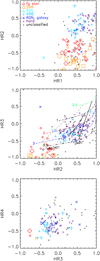 |
Fig. 2. Hardness ratio diagrams for sources detected in the four new XMM-Newton observations of the northern disc of M 31. Only sources with hardness ratio errors EHRi < 0.3 are shown. Different symbols are used for different source classes: red diamonds for foreground stars, orange squares for SNRs, cyan triangles for SSSs, light-blue crosses for X-ray binaries, and dark-blue Xs for background sources. Hard sources, which either can be AGNs or X-ray binaries, are marked with purple circles. Small symbols indicate candidates for each class, confirmed classifications are marked with large symbols. Black dots are used for unclassified sources. In HR2–HR3 diagram lines indicate the predicted position for sources with a power-law spectrum (dash-dotted lines) for Γ = 1 (black), 2 (red), 3 (blue) and a disc black-body spectrum (dashed-dot-dotted lines) for kT = 0.5 keV (black), 1.0 keV (light blue), 2.0 keV (green) for different absorbing foreground NH (thin dotted for 1020 cm−2, dashed for 1021 cm−2, and thick solid for 5 × 1021 cm−2). |
We have also calculated the hardness ratios for different types of spectral models in order to compare the distribution of sources in the hardness ratio diagram to expected spectral properties of the sources. In particular, we would like to understand if we see a difference between the XRBs in M 31 and the background sources. For AGNs we assume a power-law spectrum with Γ = 1–3 (Corral et al. 2011). The spectrum of an XRB in the hard state is also dominated by a similar power-law model. In the soft state, however, a disc black-body model will better describe the source (see, e.g. Becker & Wolff 2005; Remillard & McClintock 2006; and references therein).
There is a clear separation in HR2 between soft (foreground stars, super-soft sources [SSSs], and SNRs) and hard (XRBs and AGNs) sources, as can be seen in the upper panels of Fig. 2. In addition, there seems to be a separating trend between the sources in the background and in M 31, which are all found in the upper-right quadrant of the HR1–HR2 diagram (Fig. 2, top).
In Fig. 3 we show the count rate of each source versus hardness ratio HR2. It is obvious that the brightest sources are XRBs. In addition, the diagram reveals that the brightest XRBs are neither soft nor hard (HR2 = 0.0 − 0.5).
3.2. Spectra
We extracted spectra for all sources with a number of counts ≳100. The spectra of these sources were fitted with a power-law model. The aim of the analysis was to determine if the hard X-ray sources are members of M 31, background galaxies, or AGNs. If the column density is comparable to the Galactic foreground column density NH, MW in the direction of M 31 (Stark et al. 1992), the source is most likely located in M 31. If the column density is higher than the Galactic NH, MW the source either has an additional significantly high intrinsic NH or is located far behind M 31. The optical counterpart of the source allows us to verify whether the source is a member of M 31 or is a background source. Therefore, the column density of a yet unclassified X-ray source can help us to determine its nature.
The results of the spectral analysis are given in Tables A.2 and A.3. Table A.2 lists sources for which the optical PHAT counterparts indicate that they are members of M 31, while sources in Table A.3 have PHAT counterparts that are likely background sources. Both tables list the source ID, coordinates, the Galactic foreground NH, additional column density, photon index of the power-law spectrum, reduced χ2 with degrees of freedom, the name of the observation, and the EPIC instruments used for the spectral analysis. An additional NH was applied for sources for which the column density was higher than the Galactic column density when we first fitted the spectrum with one absorbing NH. In such a case, we froze the first NH to the Galactic NH and included a second NH which accounts for absorption in M 31 or for intrinsic absorption of the source.
If the source was detected in more than one EPIC, a simultaneous fit was performed for the source using the spectral data of all available EPIC detectors. For brighter sources that were detected in two observations, the result of the fit of the data with higher photon statistics is given in Tables A.2 and A.3. If a source was too faint for a spectral analysis in one observation, but was detected in two observations and the fluxes of the source were similar in the two observations, we used the SAS task epicspeccombine to combine the source spectra, background spectra, and ancillary response and response matrix files of each EPIC of two observations. We were thus able to improve the photon statistics of the spectra of these sources.
In Fig. 4 we show the distribution of the obtained NH and photon index Γ for the two samples. The NH is the sum of the Galactic foreground NH and the additional NH obtained by the spectral fit. The distribution of Γ seems to be similar for M 31 and background sources. The distribution of NH, by contrast, has a peak around NH = 1.5 × 1021 cm−2 corresponding to the average NH in the direction of M 31 (Milky Way and M 31 combined), and an additional distribution at higher NH for the sources suggested to be background galaxies based on PHAT data. We thus confirm the classification of these sources to be in background of M 31 through their X-ray spectra. However, this result also shows that there are background sources with NH values that are not significantly higher than the Galactic foreground. Therefore, the absorbing column density NH alone is not sufficient to separate M 31 sources from background sources.
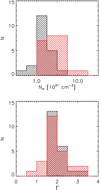 |
Fig. 4. Histograms showing the distribution of spectral fit parameters NH (Galactic and additional NH combined) and Γ for XMM-Newton sources suggested to be located in M 31 (black) and to be background sources (red) based on PHAT data. |
4. X-ray luminosity function
Using the sources from the final source list, we calculated the X-ray luminosity functions (XLFs) for the energy ranges of 0.5–2.0 keV and 2.0–10.0 keV. To estimate the contribution of background sources, we modelled the background based on the AGN XLF of the COSMOS survey (Cappelluti et al. 2009, shown in green in Fig. 5). The flux limits of the COSMOS survey were 1.7 × 10⁻¹⁵ erg cm−2 s−1 and 9.3 × 10⁻¹⁵ erg cm−2 s−1 for the 0.5–2 keV and 2–10 keV bands, respectively. We calculated the numbers of background sources by taking into account that they are more absorbed (NH = 2.3 × 1021 cm−2 for Field 1 and 3.0 × 1021 cm−2 for Field 2, Kalberla et al. 2005) than sources in the foreground of M 31 without intrinsic absorption (NH = 7 × 1020 cm−2) and extrapolated to lower fluxes. The flux was calculated assuming a power-law spectrum with a photon index of Γ = 2.0 for the softer band (0.2–5.0 keV) and Γ = 1.7 for 2.0–10.0 keV (Cappelluti et al. 2009).
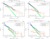 |
Fig. 5. Cumulative X-ray luminosity functions for Fields 1 (left panel) and 2 (right panel) in the bands of 0.5–2.0 keV (upper diagrams) and 2.0–10.0 keV (lower diagrams). The cumulative XLF of all observed sources without foreground stars is shown as black solid line (error ranges with dotted lines), and the XLF that has been incompleteness-corrected is shown as blue lines. The green lines show the estimated contribution of background AGNs in the field based on the study of Cappelluti et al. (2009). The XLF after subtracting the background AGN contribution is shown in orange. The XLF of classified M 31 sources is shown in red. |
In Fig. 5 we show the cumulative X-ray luminosity functions of Fields 1 and 2 in the bands of 0.5–2.0 keV and 2.0–10.0 keV calculated from the sources detected in observations OBS1 and OBS3. Sources identified as foreground stars are not included. The black lines show the cumulative XLF calculated from the detected sources, while the blue lines show the same XLFs after correcting for incompleteness. The completeness correction is based on sky-coverage function of each observation. The details can be found in Ducci et al. (2013), Saeedi et al. (2016) for example. The green line is the calculated XLF of background AGNs (Cappelluti et al. 2009) corrected for the absorption through M 31 and scaled for the observed field size. If we subtract this contribution from the corrected XLF, we should obtain the XLF of sources in M 31 (orange lines). This is compared to the XLFs of sources, which have been classified as SSSs, SNRs, or XRBs in the softer band and as XRBs in the harder band (red lines).
We have also calculated the cumulative XLFs for the merged data of OBS1 and OBS2 for Field 1 and OBS3 and OBS4 for Field 2. However, since OBS2 and OBS4 are shorter than OBS1 and OBS3, merging the results only introduces more artefacts. While merging the data helps to detect more fainter sources, it is not possible to clearly separate artefacts from real sources. In addition, both fields have been observed with large offsets of a few arcminutes between the two pointings, which increases the systematic errors due to inconsistent coverage of the fields. Therefore, we decided to use only the longer exposures.
If we compare the XLFs of Fields 1 and 2 it is obvious that more sources are detected in Field 1, which is closer to the nuclear region of M 31. The majority of these sources are probably low-mass X-ray binaries (LMXBs). We also compare the XLF to those of the XRBs in the Milky Way and the Small Magellanic Cloud (SMC) in Fig. 6. While the data of the Milky Way and the SMC cover the entire galaxy, our M 31 data only include the northern disc covering an area of 0.13 deg2. For the comparison with the Milky Way and the SMC, we scaled the XLF of M 31 to the apparent size of the disc of 1.34 deg2 based on the parameters of the luminous disc obtained by Courteau et al. (2011). The XLF of M 31 is consistent with that of the entire XRB population in the Milky Way.
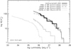 |
Fig. 6. XLFs of sources in M 31 (thick black line), X-ray binaries in the Milky Way (solid grey line), LMXBs in the Milky Way (dashed grey line), HMXBs in the Milky Way (dotted grey line), and HMXBs in the SMC (dotted light-grey line). The data for the Milky Way are taken from Grimm et al. (2002) and those for the SMC from Sturm et al. (2013). The XLF of M 31 is rescaled to the size of the entire luminous disc (see Sect. 4). |
5. Variability studies
5.1. Flux change between two epochs
We analysed the long-term variability of the objects in the cleaned source catalogue based on their EPIC count rates. Since the number of counts of all detections used for the variability study is high enough (> 20), one can assume Gaussian statistics. The search for change in flux between the two observations at a specific position is based on cross-matching of the coordinates in each epoch of the south and north fields (Fields 1 and 2, respectively). The matching radius was chosen to be 6″ to account for systematic offsets and the EPIC point spread function (PSF) especially for faint objects or those close to chip gaps. The result is shown in Fig. 7. Variable sources are marked with blue diamonds, whereas those that show no changes are indicated as black circles.
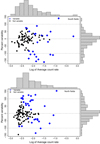 |
Fig. 7. Fractional normalised variability vs. average count rate for all sources detected in each of the two epochs of the south (Field 1, upper panel) and north (Field 2, lower panel) XMM-Newton EPIC fields. These diagrams show the change of flux between two observations, which are about half a year apart. Sources with significant variability are marked with filled blue diamonds. Non-variable sources where the real difference in their count rates is smaller than their (quadratically added) uncertainty are marked with filled black circles. Dashed grey lines mark the zero and 100% variability levels. Marginal histograms show the distributions of average count rates and fractional normalised variability. |
The corresponding count rates and source numbers are listed in Tables A.4 and A.5 for Fields 1 and 2, respectively. A source was classified as variable (blue sources in Fig. 7) if its difference in count rate between OBS1 and OBS2 or OBS3 and OBS4 (column “Difference”) was larger than three times the square root of the quadratically added uncertainties (columns “Error1” and “Error2”, or “Error3” and “Error4”). In the column “Significance”, the ratio between the “Difference” and  or
or  is given. The fractional variability in Fig. 7, listed as “Variability” and given as a percentage in Tables A.4 and A.5, was computed as the “Difference” divided by the “Mean Rate”. In total, 55 sources show significant variability between the two epochs in Fields 1 and 2. A total of 154 sources could not be matched and were detected only in one observation, even though they were observed at least twice. They are listed in Table A.6 and could be transient sources.
5.2. Light curves
5.2.1. Light curve construction and inspection
For each source in the cleaned catalogue we extracted a source and background light curve using the XMMSAS tools evselect and epiclccorr. The source region sizes were scaled based on the EPIC count rate. For pn, the background regions were determined using the new ebkgreg tool. For the MOS data we assumed a generic background annulus for a first approximation. The light curves were binned to 1 ks resolution for the few bright objects or 10 ks resolution for the many fainter objects. A standard energy band of 0.2–5.0 keV was used. Light curves of variable sources are shown and discussed in Sect. 5.4.
We made an initial classification of the variability in each background-subtracted light curve based on its variance and linear trend. In addition, we computed a smoothing fit (moving average) to identify non-linear patterns like short-term flares. We examined each light curve by eye to validate our method.
Light curves that show significant change in flux were studied in more detail in a second step. Here, we chose a tailored time binning and energy range to characterise the light curve shape in more quantitative detail. In addition, we defined source and background regions by hand to optimise the event extraction. All errors are 1σ and all upper limits are 3σ unless specifically stated otherwise. The majority of the statistical analysis was carried out within the R software environment (R Development Core Team 2011). We thus found a total of six sources that are clearly variable, two of which show flares during an observation (Sect. 5.4).
5.2.2. Variability search with the PCA
We also followed a different approach for variability detection in our sample. This approach is inspired by variability search techniques used in the optical band where accurate estimates of brightness measurement errors are often not available. We characterise each light curve with the logarithm of its average count rate and a set of 18 variability indices quantifying the light curve smoothness and scatter (for the definition of these indices see Sokolovsky et al. 2017). All the indices are designed to highlight variability, but we do not know a priori which indices will work best for our data set and variability patterns that are present in it. We therefore combine the variability indices using the principal component analysis (PCA, Pearson 1901) and identify sources that are more variable (according to the PCA combination of indices) than the majority of sources in the field. The PCA is an unsupervised, non-parametric, linear decomposition of data into new coordinates (admixture coefficients α) of an optimal set of uncorrelated axes (the eigenvectors of the variance-covariance matrix of the input data set, the principal components, hereafter, PCs). The PCs (PC1–PC18) can be thought of as variability indices, each being a linear combination of the input variability indices, while the admixture coefficients (α1–α18) are the values of these indices. The first few PCs are expected to be optimal indices. The first PC, PC1, accounts for the highest data variance possible (more widespread information), PC2 (uncorrelated to PC1) encodes most of the remaining variance, etc. High values of the first two admixture coefficients (α1 and α2) have been found to generally indicate variable sources (Sokolovsky et al. 2017; Moretti et al. 2018). For a general discussion of the impact of measurement errors on the PCA analysis see Hellton & Thoresen (2014).
The method was applied to the light curves of detections in the two M 31 fields, separately for the three EPIC detectors MOS1/2 and pn. Sources which were detected in both fields are first treated as two sources (due to largely different off-axis angles). Any source with α1 or α2 values that differ by at least three standard deviations (3σ) from the corresponding median values was considered to be a variable candidate (Fig. 8). Thus, the variability of the selected candidates is significant at > 3σ level. A total of 8, 12, and 8 sources were identified as candidate variables in MOS1, MOS2, and pn respectively, while these numbers have not been screened yet for sources which have been detected by many cameras or in two observations. Table 2 lists the final candidates for variable sources identified with this method and their classification. Sources 46, 146, and 171, which are classified as XRBs, were found to be variable. In addition, the PCA indicates that source 141, which is most likely a flaring star in the foreground (Sect. 5.4.2), and eight additional sources are probably variable (see Table 2). Of particular interest are sources 290 and 333, which have been classified as XRB candidates as a star was found in the PHAT data inside the error circle of the Chandra counterpart in each case. Source 300 is a bright SNR with a spectrum that is consistent with thermal emission from shocked plasma, with no significant hard emission detected at ≳2 keV (Sect. 6.4). It is rather unlikely that this source shows variability on timescales of ks. This indicates that using only statistical indices is not sufficient to clearly identify variable sources. Sources with clearly visible variability in their light curves are further discussed in Sect. 5.4.
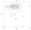 |
Fig. 8. Distribution of the admixture coefficients α1 and α2 of the PCA of MOS1 light curves. This diagram shows the variability on timescales of 1 ks. The sources marked with blue dots show significant variability consistently in all data. In this plot, source 146 appears twice since it was detected in both fields. |
Sources found to be variable based on PCA.
5.3. Pulsations
We also searched for pulsations using the barycentre-corrected events for each source. We applied different methods of timing analyses. First, we performed a  analysis (Buccheri et al. 1983, 1988) using the first and the second harmonic values of n = 1, 2 for sources that were detected on EPIC-pn. We searched for periodic signals in the period range of the Nyquist limit of 0.146 s (corresponding to twice the time resolution of EPIC-pn in full frame mode) to a period corresponding to the length of the observation. For the bright sources (> 300 counts in one EPIC), we also used the Lomb-Scargle technique for unevenly sampled time series (Scargle 1982). We calculated the Lomb-Scargle periodogram for the light curves of all observations together. However, no significant pulsation was detected for any of the sources.
5.4. Variable sources
5.4.1. Sources with variability on short timescales
Source 46 (J004344.5+412410). This is the recurrent transient 2E 161, which was first detected with the Einstein Observatory (Trinchieri & Fabbiano 1991). Its detection in our new data was first reported by Henze et al. (2016a). The source was neither detected by PFH05 nor by SPH11 in their M 31 mosaics. It was classified as a black hole candidate by Barnard et al. (2014a). A long-term X-ray light curve was published by Hofmann et al. (2013) showing indications of flare-like variability.
The source shows noticeable variability on timescales of hours in our survey data. The most prominent feature is an apparent dip at the beginning of observation 2, followed by a gradual increase in flux with potential plateaus and a continuing variability on smaller scales (Fig. 9). An analysis of different energy bands indicates that the variability happened primarily at energies below 2 keV but extended to higher energies as well. Its variability was also confirmed by the PCA.
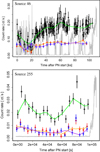 |
Fig. 9. XMM-Newton EPIC light curves of sources 46 and 255 (0.2–5.0 keV), which show variability on short timescales: pn (black), MOS1 (red), and MOS2 (blue) data points are plotted with the corresponding uncertainties. The green (pn), orange (MOS1), and purple (MOS2) curves are smoothing fits. Time resolution was optimised to the source count rate. The grey light curve shows the (scaled pn) background. |
Source 255 ([SPH11] 1551, J004456.3+415937). This is a bright, long-known ROSAT source. PFH05 and SPH11 classified it as a foreground star candidate. In the 3XMM-DR4 (the third XMM-Newton serendipitous source catalogue, Rosen et al. 2016), it was classified as non-variable, even though some EPIC light curves suggest variability. The pn light curve in Fig. 9 shows a long, slow dip of about 70 ks in duration.
5.4.2. Flare sources
Two sources (141 and 153) showed clear indications of a flaring event; both during observation 3 (which had low background up until the final 10 ks). Here we study their flux variability in detail. The light curves of the entire observation as well as a time range focused on the flare are shown in Fig. 10.
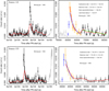 |
Fig. 10. Top: light curves of source 141 (upper panels) and source 153 (lower panels). Left panels: entire pn light curve (black, 0.2–5.0 keV) with a smoothing fit overlaid in red. The background light curve is shown in grey. MOS light curves are not shown since the photon statistics are too low. Right panels: analysis of the individual stages of the flare in a time window around it. Blue data points show the rise to maximum. The early decline (orange) in both sources can be reasonably well modelled with an exponential decline (blue fit curve; compare the red smoothing fit). The decline rates are given in units of cts s−1. Before the flare there are no indications for variability in either source. The binned count rates are entirely consistent with a Poisson process. |
Source 141 (J004417.7+415033). This source showed a clear and prominent flare detected in the pn and MOS data (Fig. 10, upper panels), which was also confirmed by PCA. The flare appears to be a primarily soft event, based on the light curves in different energy bands.
The flux rises from quiescence by an order of magnitude to peak within about 1.5–2 ks (i.e. ∼1 h; blue data points in Fig. 10, upper right). This time-scale was verified using shorter bins. Following the initial (exponential) decline, there seemed to be a re-brightening with a subsequent slow decline. This decline is consistent with a linear (green line) or exponential trend; there is no strong reason to favour either model. Source 141 is present in the catalogues of SPH11 (number 1426) and PFH05 (number 546) and was classified as a foreground star. The suggested counterpart is the object 2MASS 00441774+4150327, which has a NIR colour of J − Ks = 0.878 ± 0.058. This colour is consistent with the source being an M-type dwarf. Overall, the event is likely to have been a stellar flare.
Source 153 (J004423.0+415536). This source is also a flare object. It was located outside of MOS1 and on a chip gap of MOS2, resulting in a pn-only light curve (Fig. 10). Similar to source 141, the flare is observed in the softer band.
As can be seen in Fig. 10 (lower panels), the flux of source 153 rises from quiescence by an order of magnitude to peak within about 1–1.5 ks (i.e. ∼20 min; blue data points). Again the rise time was verified using shorter bins. The light curve suggests that immediately after the initial (exponential) decline (orange data points) the count rate remains somewhat elevated for about 6 ks until dropping back to a lower level.
During this elevated stage (about 52 ks after start) the light curve count rate appears to be Poissonian but its mean is about a factor of two higher than before the flare. A statistical rank-sum test (U-test or Mann–Whitney test; Mann & Whitney 1947) indicates that the respective distributions are significantly different at the 95% level (p-value of 0.003). This test is a non-parametric equivalent of the popular Student’s t-test and is used to check for shifts in the mean location between two (cumulative) distributions.
The significant finding indicates that the count rate remains elevated for a certain time after the flare. Source 153 is not present in any X-ray catalogue so far. We note that there is a 2MASS source, 2MASS 00442305+4155351 with J − Ks = 0.878 ± 0.058, which is a late K- or early M-type star, only 1.1″ away from our X-ray position. The 2MASS object is a likely counterpart for our X-ray source in which case the source can be classified as a foreground flaring star.
5.4.3. Sources with potential variability
Source 168 ([SPH11] 1461, J004428.7+414948). This source shows possible variability on timescales of hours (Fig. 11). Here, the signal-to-noise ratio and the flux are rather low overall but the behaviour in the three EPIC detectors looks consistent. The variability appears to be strongest in the 0.2–1 keV band.
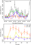 |
Fig. 11. Upper: XMM-Newton EPIC light curves (0.2–5.0 keV) of the possibly variable source 168 (pn in black, MOS1 in red, and MOS2 in blue). The colours are the same as in Fig. 9. Lower: light curves of source 168 in three energy bands: 0.2–1.0 keV (red), 1.0–2.0 keV (yellow), and 2.0–5.0 keV (blue). The variability is significant in the softest band. |
SPH11 classified this source as a possible foreground star. We have found a 2MASS source (2MASS 00442880+4149476) only 0.4″ away from the XMM-Newton position. The 3XMM catalogue contains two faint potential past detections (ML = 6 and 12; 3XMM J004428.8+414947) with no sign of variability. The NIR counterpart is a likely M-Type star with J − Ks = 0.876 ± 0.048.
5.4.4. Source with spectral variability: Source 146 (SWIFT J004420.1+413702)
The source SWIFT J004420.1+413702 was first detected as a transient source by Pietsch et al. (2008) based on observations with the Swift satellite in combination with earlier ROSAT data. The unabsorbed flux at the time of the Swift detection in 2008 was (4.6 ± 0.7)×10−13 erg s−1 cm−2 (0.5–5.0 keV) assuming an absorbed power-law model with an absorption of NH = 6.6 × 1020 cm−2 and a photon index of Γ = 1.7.
The PCA has shown that it is significantly variable. We have identified a spectral change of SWIFT J004420.1+413702, for which we have data from four epochs: June 2015 (XMM-Newton), August 2015 (XMM-Newton), October 2015 (Chandra), and January 2016 (XMM-Newton). Figure 12 shows the XMM-Newton EPIC as well as Chandra ACIS-I spectra of the source SWIFT J004420.1+413702, sorted chronologically (June 2015 [pn, MOS1], August 2015 [pn, MOS1], October 2015 [Chandra ACIS-I], January 2016 [pn, MOS2]). We fit all spectra with an absorbed power-law model. The fit results are summarised in Table 3 for the three cases: 1. both NH and Γ are free, 2. NH is fixed to the Galactic foreground value of NH = 7 × 1020 cm−2, and 3. photon index is frozen to Γ = 1.7.
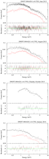 |
Fig. 12. Spectra of SWIFT J004420.1+413702 with an absorbed power-law model (NH and Γ free). For June and August 2015, and January 2016, the pn spectrum is shown in black and the MOS (1 or 2, see text) spectrum in red. |
Spectral fit results for SWIFT J004420.1+413702.
If we fix the NH to the Galactic foreground value, the photon index does not vary significantly (case 2), however, the fit statistics get worse for the spectra taken in June and August 2015, when the source was brighter.
If we assume that the shape of the intrinsic spectrum does not change (Γ = 1.7 = const, case 3) the NH values change significantly from June 2015 to January 2016, decreasing from NH = 1.1 ± 0.1 × 1021 cm−2 in August 2015 when the source was bright (absorbed flux of 3.6 ± 0.4 × 10⁻¹³ erg s−1 cm−2 and unabsorbed flux of 4.2 ± 0.5 × 10⁻¹³ erg s−1 cm−2 in the energy range of 0.5–5.0 keV) to 0.6 ± 0.2 × 1021 cm−2 about 5 months later when the source was about seven times fainter (absorbed flux of 5.4 ± 0.8 × 10⁻¹⁴ erg s−1 cm−2 and unabsorbed flux of 5.9 ± 0.8 × 10⁻¹⁴ erg s−1 cm−2).
Therefore, the source seems to show higher absorption when it is brighter and to be less absorbed when it becomes fainter without changing its intrinsic spectrum. The photon index of Γ = 1.7 is relatively inconsistent with that of a high-mass X-ray binary (HMXB); these typically have a harder spectrum. At the X-ray position, a low-mass star was found in the Chandra/PHAT survey (Williams et al. 2018), also suggesting the classification of SWIFT J004420.1+413702 as a LMXB.
6. Supernova remnants
One of the major objectives of the XMM-Newton LP observations of the northern disc of M 31 was the study of the population of SNRs. Detailed studies of several SNRs in M 31 using Chandra were performed by Kong et al. (2002a, 2003), Williams et al. (2004) for example. We had studied the SNRs detected in the XMM-Newton survey of the entire M 31 galaxy using the XMM-Newton data in X-rays and the LGS data in the optical (SPH12). We cross-correlated the new source list of the northern disc with the list of SNRs and SNR candidates of SPH12.
Lee & Lee (2014; LL14 hereafter) created a list of optical SNRs using the LGS data and classified different types of SNRs based on the optical morphology and possible progenitor. The cross-correlation of the list of X-ray SNRs with the list of LL14 has shown that not all optical SNRs are bright enough in X-rays to be detected and vice versa (see also, e.g., Bozzetto et al. 2017). All SNRs detected in the XMM-Newton LP data have HR1 > 0.0 and HR2 < 0.0, with the majority having HR2 < −0.5. X-ray sources which have an optical SNR as a counterpart and fulfill these hardness ratio criteria were newly classified as SNRs (sources 102, 213, 222, 238, and 240). In Table 4 we list the SNRs detected in the XMM-Newton LP of the northern disc. For all the SNRs and candidates in this list we extracted the spectrum. The faintest detected SNR has a flux of 4.2 × 10⁻¹⁶ erg s−1 cm−2 (0.3–10.0 keV), corresponding to a luminosity of 3.1 × 1034 erg s−1 (0.3–10.0 keV).
List of SNR detected in the new XMM-Newton LP data and their X-ray flux.
There are four sources with enough counts to make spectral fitting worthwhile (pn source counts ≳500, MOS source counts ≳150): [SPH11] 1234, 1275, 1535, and 1599. The fit results are summarised in Table 6 and the spectra are shown in Fig. 13. For the rest of the X-ray-detected SNRs, the flux was derived from the extracted spectra by assuming a thermal model (APEC). We also derived X-ray upper limits for the optical SNRs of LL14, which are listed in Table 5. For the flux calculation based on count rates, we assumed the same thermal spectrum as used by SPH12, that is, with kT = 0.2 keV, absorbed by a column density of NH = 7 × 1020 cm−2 for the Milky Way and an additional column density of NH = 1 × 1021 cm−2.
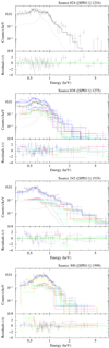 |
Fig. 13. Spectra and best fit models of the SNRs [SPH11] 1234, 1275, 1535 (APEC+APEC), and 1599 (APEC). Different colours are used to show spectra taken from different EPIC detectors and observations. |
List of optical SNRs detected by LL14 in the field of view of the new XMM-Newton LP observations and the X-ray flux upper limits (EPIC-pn).
6.1. Source 24 ([SPH11] 1234, J004327.8+411829)
This is the brightest X-ray SNR in M 31 and is also confirmed in the optical and radio. The X-ray SNR was spatially resolved with Chandra (Kong et al. 2002a). [SPH11] 1234 was located at the edge of the FOV of observation 1 and was also only observed with pn. The new spectrum can be fitted well with two APEC components (see Table 6). The two components have temperatures of 0.18 keV and 0.8 keV, indicating a mix of different plasma components. Neither a fit with a single non-equilibrium ionisation (NEI) model nor with a thermal model combined with a power law yielded a reasonable result. The two-temperature spectrum is consistent with a young SNR, with the lower-temperature component corresponding to ISM emission and the higher-temperature component to that of ejecta. Its unabsorbed flux is 9.6 × 10⁻¹⁴ erg s−1 cm−2 (0.35–2.0 keV) or 1.1 × 10⁻¹³ erg s−1 cm−2 (0.3–10.0 keV), corresponding to an intrinsic luminosity of 7.2 × 1036 erg s−1 cm−2 (0.35–2.0 keV). This source is therefore significantly fainter than the brightest SNRs in the Magellanic Clouds (van der Heyden et al. 2004; Filipović et al. 2008; Maggi et al. 2016).
Spectral fit parameters for the best fit models for the four brightest SNRs in the FOVs of the XMM-Newton LP.
6.2. Source 38 ([SPH11] 1275, J004339.1+412653)
The SNR [SPH11] 1275 was also detected in the optical and radio. The optical narrow band images of LGS and the [S II]/Hα image show an extended but rather compact source (SPH12). The spectrum of [SPH11] 1275 can be fit with two thermal components (APECs). A power-law component instead of the harder thermal component does not improve the quality of the fit. This source also seems to show both ISM and ejecta components. Its unabsorbed flux is 2.5 × 10⁻¹⁴ erg s−1 cm−2 (0.35–2.0 keV) or 2.6 × 10⁻¹⁴ erg s−1 cm−2 (0.3–10.0 keV), corresponding to an intrinsic luminosity of 1.9 × 1036 erg s−1 cm−2 (0.35–2.0 keV).
6.3. Source 242 ([SPH11] 1535, J004451.0+412906)
SPH12 have reported the detection of two stars at the position of this SNR, one detected in V and one in I. Therefore, depending on the nature of these two optical point sources, the X-ray emission might be contaminated. In the LGS narrow band images, one can see a circular shell source. The [S II]/Hα image also suggests the optical shell to be an SNR. The X-ray spectrum of [SPH11] 1535 is well fit with a thermal model consisting of two APEC components (Table 6). The temperatures are kT = 0.2 keV and 3.5 keV. The harder component can also be well modelled with a power-law with a photon index of Γ = 2.4(−0.4, +0.3), while the absorption and the softer component are the same as in the fit with a hot thermal component. The lower temperature is consistent with what has been derived for [SPH11] 1234 and 1599. Most likely this component corresponds to shocked ISM. The additional harder component either corresponds to ejecta emission with a relatively high temperature of 3.5 keV or it might indicate the existence of a pulsar wind nebula. The unabsorbed flux of this source is 1.6 × 10⁻¹⁴ erg s−1 cm−2 (0.35–2.0 keV) or 2.3 × 10⁻¹³ erg s−1 cm−2 (0.3–10.0 keV). At the distance of M 31, this corresponds to an unabsorbed luminosity of 1.2 × 1036 erg s−1 cm−2 in the energy range of 0.35–2.0 keV.
6.4. Source 300 ([SPH11] 1599, J004513.8+413615)
The spectrum of the SNR [SPH11] 1599 is well fit with one APEC component. The temperature is kT = 0.24 keV, similar to the lower temperatures of the two components for [SPH11] 1234 and 1535. Therefore, its emission seems to be dominated by that of the shocked ISM. The intrinsic absorption is high (NH = 4.1 × 1021 cm−2) and indicates that the SNR is embedded in higher density gas. The unabsorbed flux of this source is 2.1 × 10⁻¹³ erg s−1 cm−2 (0.35–2.0 keV) or 2.4 × 10⁻¹³ erg s−1 cm−2 (0.3–10.0 keV), which corresponds to an intrinsic luminosity of 1.6 × 1037 erg s−1 in the energy range of 0.35–2.0 keV, making it approximately as bright as the brightest SNR in the Magellanic Clouds or M 33 (van der Heyden et al. 2004; Filipović et al. 2008; Long et al. 2010; Maggi et al. 2016; Garofali et al. 2017).
7. Summary
We carried out deep XMM-Newton observations of two fields in the northern disc of M 31. We obtained a list of 389 sources through a combined analysis of all four observations. The new catalogue of XMM-Newton sources in the northern disc of M 31 contains 43 foreground stars and candidates, 50 background sources, 34 XRBs and candidates, and 18 SNRs and candidates.
Based on the XMM-Newton spectra of sources for which an optical counterpart was found in the PHAT data in the Chandra/PHAT survey, we find higher NH for sources which are likely background galaxies. Optical photometry combined with X-ray spectral analysis allows us to distinguish between M 31 and background sources.
There are 55 sources that show variability between the two epochs. A further 154 sources, including bright objects, are only detected in one epoch each and could be transient sources. However, there are also many faint sources with low detection likelihood among these “single-detection” objects. We have identified sources with interesting variability in their light curves: flares (sources 141 and 153), likely flares (source 168), and dips (sources 255 and 46). Based on PCA, we identify 12 sources as variable.
We detect the transient source SWIFT J004420.1+413702 and show that its flux changes significantly from June 2015 to January 2016. We analyse its spectrum at different epochs and show that the change in flux is correlated with a change in absorption. This source is classified as a LMXB, since a low-mass star was detected in the PHAT data.
The cumulative XLFs calculated for the two fields in two energy bands (0.5–2.0 keV and 2.0–10.0 keV) show that a higher number of sources are detected in the field closer to the nuclear region. More luminous sources are also found in this field. We have detected M 31 sources down to luminosities of ∼7 × 1034 erg s−1 in the softer band (0.5–2.0 keV) and to ∼4 × 1035 erg s−1 in the harder band (2.0–10.0 keV).
We perform spectral analysis of the four brightest SNRs. All four sources indicate a shocked ISM component with a temperature of kT ≈ 0.2 keV. Two SNRs have an additional thermal component with a temperature of kT ≈ 0.8 keV, which might correspond to ejecta emission.
Source 242 ([SPH11] 1535, J004451.0+412906) has a significantly harder X-ray spectrum with emission in addition to the shocked ISM component, which can either be modelled as that of a thermal plasma with a temperature of kT = 3.5 keV or with a power-law with a photon index of Γ = 2.4. This source might harbour a pulsar wind nebula and requires further investigation.
We identify five sources as new X-ray SNRs based on their hardness ratios and optical counterparts. Many of the detected SNRs are very faint in X-rays with fluxes of < 10−15 erg s−1 cm−2, corresponding to luminosities of < 1034 erg s−1 in the energy band of 0.35–2.0 keV. We thus have a sample of SNRs in the northern disc with approximately two times the sensitivity of the SNR population obtained from the XMM M 31 survey (SPH12). A deep coverage of the entire M 31 galaxy like in our new study of the northern disc will allow us to study the complete sample of faint X-ray SNRs, providing information on the environments in which SNRs originate, their interaction with the ambient ISM, and how long SNRs survive in the ISM. A detailed analysis of the ISM using the new XMM-Newton data will be presented in Kavanagh et al. (in prep.).
Acknowledgments
This research was funded by the German Bundesministerium für Wirtschaft und Technologie and the Deutsches Zentrum für Luft- und Raumfahrt (BMWi/DLR) through the grant FKZ 50 OR 1510. M.S. acknowledges support by the Deutsche Forschungsgemeinschaft (DFG) through the Heisenberg fellowship SA 2131/3-1, the Heisenberg research grant SA 2131/4-1, and the Heisenberg professor grant SA 2131/5-1. M.S., B.W., and P.P. acknowledge partial support for this research through the Chandra Research Visitors Program. M.H. acknowledges the support of the Spanish Ministry of Economy and Competitiveness (MINECO) under the grant FDPI-2013-16933 as well as the support of the Generalitat de Catalunya/CERCA programme. Support for B.F.W. was provided by Chandra Award Number GO5-16085X issued by the Chandra X-ray Observatory Center, which is operated by the Smithsonian Astrophysical Observatory for and on behalf of the National Aeronautics and Space Administration under contract NAS8-03060. D.H., A.K., and K.S. are supported by the European Space Agency (ESA) under the “Hubble Catalog of Variables” programme, contract No. 4000112940. D.B. acknowledges partial support from the DFG through project ISM-SPP 1573. This research has made use of the the SIMBAD database, and the VizieR catalogue access tool operated at CDS, Strasbourg, France.
References
- Barnard, R., Stiele, H., Hatzidimitriou, D., et al. 2008, ApJ, 689, 1215 [NASA ADS] [CrossRef] [Google Scholar]
- Barnard, R., Garcia, M., & Murray, S. S. 2012, ApJ, 757, 40 [NASA ADS] [CrossRef] [Google Scholar]
- Barnard, R., Garcia, M. R., Primini, F., et al. 2014a, ApJ, 780, 83 [NASA ADS] [CrossRef] [Google Scholar]
- Barnard, R., Garcia, M. R., Primini, F., & Murray, S. S. 2014b, ApJ, 791, 33 [NASA ADS] [CrossRef] [Google Scholar]
- Becker, P. A., & Wolff, M. T. 2005, ApJ, 630, 465 [NASA ADS] [CrossRef] [Google Scholar]
- Block, D. L., Bournaud, F., Combes, F., et al. 2006, Nature, 443, 832 [NASA ADS] [CrossRef] [Google Scholar]
- Bozzetto, L. M., Filipović, M. D., Vukotić, B., et al. 2017, ApJS, 230, 2 [NASA ADS] [CrossRef] [Google Scholar]
- Brinks, E., & Shane, W. W. 1984, A&AS, 55, 179 [NASA ADS] [Google Scholar]
- Brown, T. M., Smith, E., Ferguson, H. C., et al. 2006, ApJ, 652, 323 [NASA ADS] [CrossRef] [Google Scholar]
- Buccheri, R., Bennett, K., Bignami, G. F., et al. 1983, A&A, 128, 245 [NASA ADS] [Google Scholar]
- Buccheri, R., Maccarone, M. C., Sacco, B., & di Gesu, V. 1988, A&A, 201, 194 [NASA ADS] [Google Scholar]
- Cappelluti, N., Brusa, M., Hasinger, G., et al. 2009, A&A, 497, 635 [NASA ADS] [CrossRef] [EDP Sciences] [Google Scholar]
- Conn, A. R., McMonigal, B., Bate, N. F., et al. 2016, MNRAS, 458, 3282 [NASA ADS] [CrossRef] [Google Scholar]
- Corral, A., Della Ceca, R., Caccianiga, A., et al. 2011, A&A, 530, A42 [NASA ADS] [CrossRef] [EDP Sciences] [Google Scholar]
- Courteau, S., Widrow, L. M., McDonald, M., et al. 2011, ApJ, 739, 20 [NASA ADS] [CrossRef] [Google Scholar]
- Dalcanton, J. J., Williams, B. F., Lang, D., et al. 2012, ApJS, 200, 18 [NASA ADS] [CrossRef] [Google Scholar]
- Dame, T. M., Koper, E., Israel, F. P., & Thaddeus, P. 1993, ApJ, 418, 730 [NASA ADS] [CrossRef] [Google Scholar]
- Ducci, L., Sasaki, M., Haberl, F., & Pietsch, W. 2013, A&A, 553, A7 [NASA ADS] [CrossRef] [EDP Sciences] [Google Scholar]
- Filipović, M. D., Haberl, F., Winkler, P. F., et al. 2008, A&A, 485, 63 [NASA ADS] [CrossRef] [EDP Sciences] [Google Scholar]
- Fritz, J., Gentile, G., Smith, M. W. L., et al. 2012, A&A, 546, A34 [NASA ADS] [CrossRef] [EDP Sciences] [Google Scholar]
- Galvin, T. J., & Filipovic, M. D. 2014, Serb. Astron. J., 189, 15 [NASA ADS] [CrossRef] [Google Scholar]
- Galvin, T. J., Filipovic, M. D., Crawford, E. J., et al. 2012, Serb. Astron. J., 184, 41 [Google Scholar]
- Garofali, K., Williams, B. F., Plucinsky, P. P., et al. 2017, MNRAS, 472, 308 [NASA ADS] [CrossRef] [Google Scholar]
- Gordon, K. D., Bailin, J., Engelbracht, C. W., et al. 2006, ApJ, 638, L87 [Google Scholar]
- Grimm, H.-J., Gilfanov, M., & Sunyaev, R. 2002, A&A, 391, 923 [NASA ADS] [CrossRef] [EDP Sciences] [Google Scholar]
- Hellton, K. H., & Thoresen, M. 2014, Scand. J. Stat., 41, 1051 [CrossRef] [Google Scholar]
- Henze, M., Sasaki, M., Haberl, F., & Hatzidimitriou, D. 2015a, ATel, 8227 [Google Scholar]
- Henze, M., Sasaki, M., Haberl, F., & Hatzidimitriou, D. 2015b, ATel, 8228 [Google Scholar]
- Henze, M., Sasaki, M., Haberl, F., Williams, B. F., & Hatzidimitriou, D. 2016a, ATel, 8827 [Google Scholar]
- Henze, M., Sasaki, M., Haberl, F., Williams, B. F., & Hatzidimitriou, D. 2016b, ATel, 8825 [Google Scholar]
- Henze, M., Sasaki, M., & Haberl, F. 2016c, ATel, 8826 [Google Scholar]
- Hofmann, F., Pietsch, W., Henze, M., et al. 2013, A&A, 555, A65 [NASA ADS] [CrossRef] [EDP Sciences] [Google Scholar]
- Kaaret, P. 2002, ApJ, 578, 114 [NASA ADS] [CrossRef] [Google Scholar]
- Kalberla, P. M. W., Burton, W. B., Hartmann, D., et al. 2005, A&A, 440, 775 [NASA ADS] [CrossRef] [EDP Sciences] [Google Scholar]
- Kong, A. K. H., Garcia, M. R., Primini, F. A., & Murray, S. S. 2002a, ApJ, 580, L125 [NASA ADS] [CrossRef] [Google Scholar]
- Kong, A. K. H., Garcia, M. R., Primini, F. A., et al. 2002b, ApJ, 577, 738 [NASA ADS] [CrossRef] [Google Scholar]
- Kong, A. K. H., Sjouwerman, L. O., Williams, B. F., Garcia, M. R., & Dickel, J. R. 2003, ApJ, 590, L21 [NASA ADS] [CrossRef] [Google Scholar]
- Lee, J. H., & Lee, M. G. 2014, ApJ, 786, 130 [NASA ADS] [CrossRef] [Google Scholar]
- Long, K. S., Blair, W. P., Winkler, P. F., et al. 2010, ApJS, 187, 495 [NASA ADS] [CrossRef] [Google Scholar]
- Maccarone, T. J., Yukita, M., Hornschemeier, A., et al. 2016, MNRAS, 458, 3633 [NASA ADS] [CrossRef] [Google Scholar]
- Maggi, P., Haberl, F., Kavanagh, P. J., et al. 2016, A&A, 585, A162 [NASA ADS] [CrossRef] [EDP Sciences] [Google Scholar]
- Mann, H. B., & Whitney, D. R. 1947, Ann. Math. Stat., 18, 50 [CrossRef] [Google Scholar]
- Massey, P., Hodge, P. W., Holmes, S., et al. 2002, Amer. Astron. Soc. Meet. Abstr., BAAS, 34, 1272 [NASA ADS] [Google Scholar]
- Massey, P., Olsen, K. A. G., Hodge, P. W., et al. 2006, AJ, 131, 2478 [NASA ADS] [CrossRef] [Google Scholar]
- Monet, D. G., Levine, S. E., Canzian, B., et al. 2003, AJ, 125, 984 [NASA ADS] [CrossRef] [Google Scholar]
- Moretti, M. I., Hatzidimitriou, D., Karampelas, A., et al. 2018, MNRAS, 477, 2664 [NASA ADS] [CrossRef] [Google Scholar]
- Osborne, J. P., Borozdin, K. N., Trudolyubov, S. P., et al. 2001, A&A, 378, 800 [NASA ADS] [CrossRef] [EDP Sciences] [Google Scholar]
- Pearson, K. 1901, Phil. Mag., 2, 559 [Google Scholar]
- Pietsch, W., Freyberg, M., & Haberl, F. 2005, A&A, 434, 483 [NASA ADS] [CrossRef] [EDP Sciences] [Google Scholar]
- Pietsch, W., Freyberg, M., Henze, M., Stiele, H., & Immler, S. 2008, ATel, 1671 [Google Scholar]
- R Development Core Team 2011, R: A Language and Environment for Statistical Computing, R Foundation for Statistical Computing, Vienna, Austria [Google Scholar]
- Remillard, R. A., & McClintock, J. E. 2006, ARA&A, 44, 49 [NASA ADS] [CrossRef] [Google Scholar]
- Rosen, S. R., Webb, N. A., Watson, M. G., et al. 2016, A&A, 590, A1 [NASA ADS] [CrossRef] [EDP Sciences] [Google Scholar]
- Saeedi, S., Sasaki, M., & Ducci, L. 2016, A&A, 586, A64 [NASA ADS] [CrossRef] [EDP Sciences] [Google Scholar]
- Sasaki, M., Pietsch, W., Haberl, F., et al. 2012, A&A, 544, A144 [NASA ADS] [CrossRef] [EDP Sciences] [Google Scholar]
- Scargle, J. D. 1982, ApJ, 263, 835 [NASA ADS] [CrossRef] [Google Scholar]
- Skrutskie, M. F., Cutri, R. M., Stiening, R., et al. 2006, AJ, 131, 1163 [NASA ADS] [CrossRef] [Google Scholar]
- Smith, M. W. L., Eales, S. A., Gomez, H. L., et al. 2012, ApJ, 756, 40 [NASA ADS] [CrossRef] [Google Scholar]
- Sokolovsky, K. V., Gavras, P., Karampelas, A., et al. 2017, MNRAS, 464, 274 [NASA ADS] [CrossRef] [Google Scholar]
- Stark, A. A., Gammie, C. F., Wilson, R. W., et al. 1992, ApJS, 79, 77 [NASA ADS] [CrossRef] [Google Scholar]
- Stiele, H., Pietsch, W., Haberl, F., & Freyberg, M. 2008, A&A, 480, 599 [NASA ADS] [CrossRef] [EDP Sciences] [Google Scholar]
- Stiele, H., Pietsch, W., Haberl, F., et al. 2011, A&A, 534, A55 [NASA ADS] [CrossRef] [EDP Sciences] [Google Scholar]
- Strüder, L., Briel, U., Dennerl, K., et al. 2001, A&A, 365, L18 [NASA ADS] [CrossRef] [EDP Sciences] [Google Scholar]
- Sturm, R., Haberl, F., Pietsch, W., et al. 2013, A&A, 558, A3 [NASA ADS] [CrossRef] [EDP Sciences] [Google Scholar]
- Supper, R., Hasinger, G., Pietsch, W., et al. 1997, A&A, 317, 328 [NASA ADS] [Google Scholar]
- Supper, R., Hasinger, G., Lewin, W. H. G., et al. 2001, A&A, 373, 63 [NASA ADS] [CrossRef] [EDP Sciences] [Google Scholar]
- Trinchieri, G., & Fabbiano, G. 1991, ApJ, 382, 82 [NASA ADS] [CrossRef] [Google Scholar]
- Trudolyubov, S., Kotov, O., Priedhorsky, W., Cordova, F., & Mason, K. 2005, ApJ, 634, 314 [NASA ADS] [CrossRef] [Google Scholar]
- Turner, M. J. L., Abbey, A., Arnaud, M., et al. 2001, A&A, 365, L27 [NASA ADS] [CrossRef] [EDP Sciences] [Google Scholar]
- van der Heyden, K. J., Bleeker, J. A. M., & Kaastra, J. S. 2004, A&A, 421, 1031 [NASA ADS] [CrossRef] [EDP Sciences] [Google Scholar]
- van Speybroeck, L., Epstein, A., Forman, W., et al. 1979, ApJ, 234, L45 [NASA ADS] [CrossRef] [Google Scholar]
- Vulic, N., Gallagher, S. C., & Barmby, P. 2016, MNRAS, 461, 3443 [NASA ADS] [CrossRef] [Google Scholar]
- Williams, B. F. 2003, AJ, 126, 1312 [NASA ADS] [CrossRef] [Google Scholar]
- Williams, B. F., Sjouwerman, L. O., Kong, A. K. H., et al. 2004, ApJ, 615, 720 [NASA ADS] [CrossRef] [Google Scholar]
- Williams, B. F., Naik, S., Garcia, M. R., & Callanan, P. J. 2006, ApJ, 643, 356 [NASA ADS] [CrossRef] [Google Scholar]
- Williams, B. F., Hatzidimitriou, D., Green, J., et al. 2014a, MNRAS, 443, 2499 [NASA ADS] [CrossRef] [Google Scholar]
- Williams, B. F., Lang, D., Dalcanton, J. J., et al. 2014b, ApJS, 215, 9 [NASA ADS] [CrossRef] [Google Scholar]
- Williams, B. F., Dolphin, A. E., Dalcanton, J. J., et al. 2017, ApJ, 846, 145 [NASA ADS] [CrossRef] [Google Scholar]
- Williams, B. F., Lazzarini, M., Plucinsky, P., et al. 2018, ApJS, in press [arXiv:1808.10487] [Google Scholar]
All Tables
List of optical SNRs detected by LL14 in the field of view of the new XMM-Newton LP observations and the X-ray flux upper limits (EPIC-pn).
Spectral fit parameters for the best fit models for the four brightest SNRs in the FOVs of the XMM-Newton LP.
All Figures
|
Fig. 1. Left: exposure-corrected mosaic image in the energy band 0.2–1.0 keV. Marked sources are: cyan (XRBs and candidates), yellow (SNRs and candidates), red (SSSs and candidates). XRBs and candidates, for which a spectral analysis was performed, are additionally marked with a circle (see Sect. 3.2). Background sources with fitted spectra are marked with magenta circles. Right: exposure-corrected mosaic images of the XMM-Newton LP observations of the northern disc of M 31 in three colours (red: 0.2–1.0 keV, green: 1.0–2.0 keV, blue = 2.0–12.0 keV) with the footprints of the new Chandra survey and the PHAT survey shown by solid green line and dashed magenta line, respectively. All images are shown in log-scale. |
| In the text | |
|
Fig. 2. Hardness ratio diagrams for sources detected in the four new XMM-Newton observations of the northern disc of M 31. Only sources with hardness ratio errors EHRi < 0.3 are shown. Different symbols are used for different source classes: red diamonds for foreground stars, orange squares for SNRs, cyan triangles for SSSs, light-blue crosses for X-ray binaries, and dark-blue Xs for background sources. Hard sources, which either can be AGNs or X-ray binaries, are marked with purple circles. Small symbols indicate candidates for each class, confirmed classifications are marked with large symbols. Black dots are used for unclassified sources. In HR2–HR3 diagram lines indicate the predicted position for sources with a power-law spectrum (dash-dotted lines) for Γ = 1 (black), 2 (red), 3 (blue) and a disc black-body spectrum (dashed-dot-dotted lines) for kT = 0.5 keV (black), 1.0 keV (light blue), 2.0 keV (green) for different absorbing foreground NH (thin dotted for 1020 cm−2, dashed for 1021 cm−2, and thick solid for 5 × 1021 cm−2). |
| In the text | |
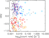 |
Fig. 3. Hardness ratio HR2 over logarithm of count rate (s−1). Same symbols as in Fig. 2 are used. |
| In the text | |
|
Fig. 4. Histograms showing the distribution of spectral fit parameters NH (Galactic and additional NH combined) and Γ for XMM-Newton sources suggested to be located in M 31 (black) and to be background sources (red) based on PHAT data. |
| In the text | |
|
Fig. 5. Cumulative X-ray luminosity functions for Fields 1 (left panel) and 2 (right panel) in the bands of 0.5–2.0 keV (upper diagrams) and 2.0–10.0 keV (lower diagrams). The cumulative XLF of all observed sources without foreground stars is shown as black solid line (error ranges with dotted lines), and the XLF that has been incompleteness-corrected is shown as blue lines. The green lines show the estimated contribution of background AGNs in the field based on the study of Cappelluti et al. (2009). The XLF after subtracting the background AGN contribution is shown in orange. The XLF of classified M 31 sources is shown in red. |
| In the text | |
|
Fig. 6. XLFs of sources in M 31 (thick black line), X-ray binaries in the Milky Way (solid grey line), LMXBs in the Milky Way (dashed grey line), HMXBs in the Milky Way (dotted grey line), and HMXBs in the SMC (dotted light-grey line). The data for the Milky Way are taken from Grimm et al. (2002) and those for the SMC from Sturm et al. (2013). The XLF of M 31 is rescaled to the size of the entire luminous disc (see Sect. 4). |
| In the text | |
|
Fig. 7. Fractional normalised variability vs. average count rate for all sources detected in each of the two epochs of the south (Field 1, upper panel) and north (Field 2, lower panel) XMM-Newton EPIC fields. These diagrams show the change of flux between two observations, which are about half a year apart. Sources with significant variability are marked with filled blue diamonds. Non-variable sources where the real difference in their count rates is smaller than their (quadratically added) uncertainty are marked with filled black circles. Dashed grey lines mark the zero and 100% variability levels. Marginal histograms show the distributions of average count rates and fractional normalised variability. |
| In the text | |
|
Fig. 8. Distribution of the admixture coefficients α1 and α2 of the PCA of MOS1 light curves. This diagram shows the variability on timescales of 1 ks. The sources marked with blue dots show significant variability consistently in all data. In this plot, source 146 appears twice since it was detected in both fields. |
| In the text | |
|
Fig. 9. XMM-Newton EPIC light curves of sources 46 and 255 (0.2–5.0 keV), which show variability on short timescales: pn (black), MOS1 (red), and MOS2 (blue) data points are plotted with the corresponding uncertainties. The green (pn), orange (MOS1), and purple (MOS2) curves are smoothing fits. Time resolution was optimised to the source count rate. The grey light curve shows the (scaled pn) background. |
| In the text | |
|
Fig. 10. Top: light curves of source 141 (upper panels) and source 153 (lower panels). Left panels: entire pn light curve (black, 0.2–5.0 keV) with a smoothing fit overlaid in red. The background light curve is shown in grey. MOS light curves are not shown since the photon statistics are too low. Right panels: analysis of the individual stages of the flare in a time window around it. Blue data points show the rise to maximum. The early decline (orange) in both sources can be reasonably well modelled with an exponential decline (blue fit curve; compare the red smoothing fit). The decline rates are given in units of cts s−1. Before the flare there are no indications for variability in either source. The binned count rates are entirely consistent with a Poisson process. |
| In the text | |
|
Fig. 11. Upper: XMM-Newton EPIC light curves (0.2–5.0 keV) of the possibly variable source 168 (pn in black, MOS1 in red, and MOS2 in blue). The colours are the same as in Fig. 9. Lower: light curves of source 168 in three energy bands: 0.2–1.0 keV (red), 1.0–2.0 keV (yellow), and 2.0–5.0 keV (blue). The variability is significant in the softest band. |
| In the text | |
|
Fig. 12. Spectra of SWIFT J004420.1+413702 with an absorbed power-law model (NH and Γ free). For June and August 2015, and January 2016, the pn spectrum is shown in black and the MOS (1 or 2, see text) spectrum in red. |
| In the text | |
|
Fig. 13. Spectra and best fit models of the SNRs [SPH11] 1234, 1275, 1535 (APEC+APEC), and 1599 (APEC). Different colours are used to show spectra taken from different EPIC detectors and observations. |
| In the text | |
Current usage metrics show cumulative count of Article Views (full-text article views including HTML views, PDF and ePub downloads, according to the available data) and Abstracts Views on Vision4Press platform.
Data correspond to usage on the plateform after 2015. The current usage metrics is available 48-96 hours after online publication and is updated daily on week days.
Initial download of the metrics may take a while.