| Issue |
A&A
Volume 618, October 2018
|
|
|---|---|---|
| Article Number | A171 | |
| Number of page(s) | 35 | |
| Section | Stellar structure and evolution | |
| DOI | https://doi.org/10.1051/0004-6361/201833177 | |
| Published online | 01 November 2018 | |
Warm CO in evolved stars from the THROES catalogue
I. Herschel-PACS spectroscopy of O-rich envelopes⋆
1 Department of Astrophysics, Astrobiology Centre (CSIC-INTA), ESAC campus, PO Box 78, 28691 Villanueva de la Cañada,Madrid, Spain
e-mail: This email address is being protected from spambots. You need JavaScript enabled to view it.
2 European Space Astronomy Centre, European Space Agency, PO Box 78, 28691 Villanueva de la Cañada, Madrid, Spain
3 Institute for Solar Physics, Department of Astronomy, Stockholm University, AlbaNova University Centre, 106 91 Stockholm, Sweden
Received:
6
April
2018
Accepted:
1
August
2018
Abstract
In this work (Paper I), we analyse Herschel-PACS spectroscopy for a subsample of 23 O-rich and 3 S-type evolved stars, in different evolutionary stages from the asymptotic giant branch (AGB) to the planetary nebula (PN) phase, from the THROES catalogue. (C-rich targets are separately studied in Paper II). The broad spectral range covered by PACS (∼55–210 μm) includes a large number of high-J CO lines, from J = 14 − 13 to J = 45 − 44 (v = 0), that allow us to study the warm inner layers of the circumstellar envelopes (CSEs) of these objects, at typical distances from the star of ≈1014–1015 cm and ≈1016 cm for AGBs and post-AGB-PNe, respectively. We have generated CO rotational diagrams for each object to derive the rotational temperature, total mass within the CO-emitting region and average mass-loss rate during the ejection of these layers. We present first order estimations of these basic physical parameters using a large number of high-J CO rotational lines, with upper-level energies from Eup ∼ 580 to 5000 K, for a relatively big set of evolved low-to-intermediate mass stars in different AGB-to-PN evolutionary stages. We derive rotational temperatures ranging from Trot ∼ 200 to 700 K, with typical values around 500 K for AGBs and systematically lower, ∼200 K, for objects in more advanced evolutionary stages (post-AGBs and PNe). Our values of Trot are one order or magnitude higher than the temperatures of the outer CSE layers derived from low-J CO line studies. The total mass of the inner CSE regions where the PACS CO lines arise is found to range from MH2 ∼ 10−6 to ≈10−2 M⊙, which is expected to represent a small fraction of the total CSE mass. The mass-loss rates estimated are in the range Ṁ ∼ 10−7 − 10−4 M⊙yr−1, in agreement (within uncertainties) with values found in the literature. We find a clear anticorrelation between MH2 and Ṁ vs. Trot that probably results from a combination of most efficient line cooling and higher line opacities in high mass-loss rate objects. For some strong CO emitters in our sample, a double temperature (hot and warm) component is inferred. The temperatures of the warm and hot components are ∼400–500 K and ∼600–900 K, respectively. The mass of the warm component (∼10−5–8 × 10⁻² M⊙) is always larger than that of the hot component, by a factor of between two and ten. The warm-to-hot MH2 and Trot ratios in our sample are correlated and are consistent with an average temperature radial profile of ∝ r−0.5 ± 0.1, that is, slightly shallower than in the outer envelope layers, in agreement with recent studies.
Key words: stars: AGB and post-AGB / circumstellar matter / stars: mass-loss / planetary nebulae: general / infrared: stars / stars: evolution
Herschel is an ESA space observatory with science instruments provided by European-led Principal Investigator consortia and with important participation from NASA.
Note to the Reader: Following the publication of the corrigendum, the article was corrected on November 21, 2018.
© ESO 2018
1. Introduction
The asymptotic giant branch (AGB) is one of the late stages in the evolution of low and intermediate mass stars (1 M ⊙ ≲ M ≲ 8 M⊙). At this phase, stars are very luminous (∼104 L⊙) and cool, with effective temperatures ranging from Teff ∼ 2000 to 4000 K. The stellar radius of a typical AGB star is of about 1 AU, i.e. R⋆ ≈ 1013 cm. AGB stars are dominated by an intense mass loss process with rates that range, typically, between 10−7 and 10−4 M⊙ yr−1. For complete reviews see, for example, Habing (1996), Herwig (2005), Höfner & Olofsson (2018).
The vigorous mass loss generates a circumstellar envelope (CSE) of gas and dust around these evolved objects. The mass loss is thought to be produced by the combination of two mechanisms: pulsations and radiation pressure on dust (Bowen 1988; Simis et al. 2001). Both mechanisms work together driving a slow, dense stellar wind. The wind is strongly accelerated from the dust condensation region (at a few stellar radii, ≈1014 cm), reaching terminal velocities of about 5 to 25 km s−1 at distances from the star of ≳10–20 R⋆. The temperature of the gas decreases along the CSE from 2000–2500 K, close to the stellar atmosphere, to ∼1000 K in the dust condensation region, and progressively falling down to just a few tens of K in the most external envelope layers, at ≈1016 − 1017 cm (e.g. Decin 2012).
The material ejected due to the mass loss process, is expected to enrich the interstellar medium (ISM) with stellar nucleosynthesis products. It is believed that about half of the elements heavier than Fe are formed in the AGB phase (Herwig 2005). The analysis of the molecular products found in the AGB CSEs is very useful to derive information on the nucleosynthesis history of the central star and to improve our current understanding of the complex circumstellar chemistry (e.g. Millar 2016).
The relative abundance of carbon and oxygen in the CSE completely determines the dominant chemistry of these envelopes. According to the ratio of carbon over oxygen atoms, we identify envelopes with a carbon-rich (C/O > 1) or oxygen-rich (C/O < 1) chemistry, with a few objects (known as S-stars) showing C/O ratios very close to unity. This chemical branching is very important and depends on the nucleosynthesis processes that have taken place in the interior of these stars during their AGB evolution, which are basically determined by the mass of the progenitor star and its initial metallicity. All stars are born with a C/O ∼ 0.5 and therefore O-rich. However, this chemical composition may change during their AGB evolution. According to theoretical models (Marigo et al. 2003; Karakas et al. 2009), low-mass progenitors (M < 2 M⊙) remain as O-rich objects throughout the whole AGB evolution, while those stars with higher initial masses, between 2 and 4 M⊙, may become C-rich objects during the AGB phase due to the thermal pulses and convective processes (dredge-ups) that enrich the surface of the AGB star with carbon, produced as a result of nuclear reactions. Finally, the most massive objects (AGB stars with initial masses in the range 4 M⊙ < M < 8 M⊙) remain also O-rich throughout their evolution in the AGB as they do not produce so much carbon, instead they convert carbon into nitrogen via the CN cycle (in a process known as hot bottom burning).
After the AGB phase the convective envelope is expelled and the hot core starts to ionize the surrounding material. When the bulk of the gas in the CSE is ionized the object is recognized as a planetary nebula (PN), see Kwok (2005).
The transition phase between AGBs and PNe is called the post-AGB phase. It is a very fast (≈103 − 104 yr) phase when the shell, formed in the AGB phase, detaches from the central star and the spherical symmetry is usually broken due to the effect of the onset of fast bipolar or multi-polar winds (Balick & Frank 2002).
The CO molecule is one of the most abundant species found in these objects as it is quickly and easily formed from the O and C atoms present in the envelope and it is also the most stable at the typical conditions found in these envelopes, CO molecules develop strong rotational emission lines which are very useful to trace the physical properties of the molecular envelopes around evolved stars in different evolutionary stages, from the AGB to the PN phase.
The molecular emission of CO has been studied over the last decades mainly at mm and sub-mm wavelength ranges using the low-J transitions that trace outer (> 1016 cm) relatively cold (10–50 K) regions of the CSE (Bujarrabal 1999; Schöier & Olofsson 2001; Teyssier et al. 2006; Ramstedt et al. 2009). Studying the hotter layers of the envelope, presumably closer to the central star, traced by high-J CO transitions has only been possible with space telescopes like the Infrared Space Observatory (ISO; see, for example Justtanont et al. 2000) and in more recent times with Herschel, particularly, making use of PACS spectroscopy data (see, Groenewegen et al. 2011; Ueta et al. 2014).
Here, we analyse, in a uniform and systematic way, PACS spectroscopy data of a sample of O-rich (and a few S-type) evolved stars from the THROES catalogue (Ramos-Medina et al. 2018). We focus our study on the high-excitation rotational transitions of the CO molecule detected in these stars. In Sect. 2, a general description of our sample is provided. After that, in Sect. 3, we present the main characteristics of the PACS instrument and provide a brief description of the major data reduction steps. In Sect. 4 we show the principal observational results, including our measurements of the CO line fluxes. The rotational diagram (RD) analysis method used in this work and the results derived can be found in Sects. 5 and 6, respectively. The analysis of our results is presented in Sect. 7. Finally, in Sect. 8 we summarize our main conclusions.
2. Sample information
In this work we have studied 26 evolved stars at different evolutionary stages, from the AGB to PN phase, taken from the THROES catalogue (Ramos-Medina et al. 2018). In its current version, the THROES catalogue contains PACS spectroscopic cubes for a total of 114 low-to-intermediate mass evolved stars. In this study, we focus on non C-rich targets, with most of our sources being O-rich objects but also including a few S-type AGB stars (Table D.1). Sources with a dominant C-rich chemistry are studied separately by da Silva Santos et al. (in prep., Paper II). Our sources are grouped in five main categories as originally defined in the THROES catalogue: classical O-rich and S-type AGB stars, OH/IR stars (strong far-IR emitters with intense OH maser lines, typically late-AGB or early post-AGB stars heavily obscured by dust at optical wavelengths), post-AGB objects, and PNe. For this study, we have selected objects with a minimum of three CO transitions detected with a ratio of S/N > 3, a total of 26 out of 66 non C-rich targets in the THROES catalogue.
In Fig. 1 we present IRAS fluxes and colours of the sources of our sample in comparison with the rest of objects (C-rich or CO non-detections of any chemical type) contained in the THROES catalogue. IRAS colours in this diagram are defined as: ![Mathematical equation: $ [12]{-}[25]=2.5\log_{10}\frac{\mathrm{IRAS}_{25}}{\mathrm{IRAS}_{12}} $](/articles/aa/full_html/2018/10/aa33177-18/aa33177-18-eq1.gif) and
and ![Mathematical equation: $ [25]{-}[60]=2.5\log_{10}\frac{\mathrm{IRAS}_{60}}{\mathrm{IRAS}_{25}} $](/articles/aa/full_html/2018/10/aa33177-18/aa33177-18-eq2.gif) . In the colour–colour diagram, the sources included in the THROES catalogue follow a well-known evolutionary sequence, with the AGBs located at the bottom left region (boxes: I, II, IIIa and VII) and the post-AGBs and PNe occupying the upper right area (boxes: V and VIII); more details can be found in van der Veen & Habing (1988). We note that the only OH/IR star located close to other PNe in region V is OH 231.8+4.2, which is a peculiar AGB star with a massive outflow with physical and chemical particularities uncommon for the AGB stage but approaching those of post-AGB objects (e.g. Alcolea et al. 2001; Sánchez Contreras et al. 2015).
. In the colour–colour diagram, the sources included in the THROES catalogue follow a well-known evolutionary sequence, with the AGBs located at the bottom left region (boxes: I, II, IIIa and VII) and the post-AGBs and PNe occupying the upper right area (boxes: V and VIII); more details can be found in van der Veen & Habing (1988). We note that the only OH/IR star located close to other PNe in region V is OH 231.8+4.2, which is a peculiar AGB star with a massive outflow with physical and chemical particularities uncommon for the AGB stage but approaching those of post-AGB objects (e.g. Alcolea et al. 2001; Sánchez Contreras et al. 2015).
All the objects of our sample except two, IRAS 17347-3139 and NGC 6537, have previous estimations of the mass loss rate but using low-J CO lines detected in the sub-millimetre and millimetre ranges (see Table D.2). Only for six objects namely, NML Tau, TX Cam, R Dor, R Cas, W Hya and W Aql, the mass loss rates provided come from recent works (Danilovich et al. 2014; Khouri et al. 2014; Maercker et al. 2016; Van de Sande et al. 2018) which are based on detailed non-local thermal equilibrium (non-LTE) radiative transfer models which make use of a combination of different sets of CO lines taken from several telescopes and including HIFI and PACS observations that, eventually, cover CO rotational lines up to J = 24 − 23. We have paid particular attention to the mass loss rates estimations derived in these works in order to test the results obtained with the rotational diagram method, used in this paper.
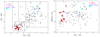 |
Fig. 1. IRAS colour–colour diagram (left) and 100 μm flux vs. [12]−[25] IRAS colour (right) of the THROES targets with good quality IRAS data (Quality Flag = 3) in the 12, 25, 60 and 100 μm bands. The colour–colour diagram is divided in different boxes where sources with common characteristics and evolutionary stages are located (see van der Veen & Habing 1988, for details). Objects with CO line detections, studied in this work, are highlighted using the symbol and colour code shown in the figure. In the rest of the plots presented throughout this paper, AGBs, OH/IRs, post-AGBs and PNe are coloured and symbol-coded as indicated in this figure. |
3. Observations and data reduction
PACS (Poglitsch et al. 2010) is an instrument onboard Herschel (Pilbratt et al. 2010) with photometric and spectroscopic capabilities in the FIR wavelength region. The PACS spectrometer covers the wavelength range from 51 to 210 μm in two different channels that operate simultaneously in the blue (51–105 μm) and red (102–220 μm) bands. The Field of View (FoV) covers a 47″×47″ region in the sky, it is structured in an array of 5 × 5 spatial pixels (“spaxels”), each spaxel is a 9.4″×9.4″ square. PACS provides a resolving power between 5500 and 940 (i.e. a spectral resolution of 55–320 km s−1) at short and long wavelengths, respectively, and the point spread function (PSF) of the PACS spectrometer ranges from ∼9″ in the blue band to ∼13″ in the red band. The PSF is described in da Silva Santos (2016) and Bocchio et al. (2016). Complete details about PACS instrument can be found in the PACS Observer’s Manual1.
In this work we have used one-dimensional (1D) PACS spectra, integrated over the emitting source, taken from the THROES catalogue (Ramos-Medina et al. 2018). THROES is a web-based catalogue that contains fully reduced PACS spectra, in 3D cubes structure (FITS files) and 1D spectra format (FITS and CSV files), for 114 low-to-intermediate mass evolved stars, covering a range of evolutionary stages from the AGB to the PN phase. The THROES catalogue is public and can be accessed online2.
The main goal of the THROES project was the production of enhanced PACS spectroscopic data through the systematic careful interactive reprocessing, for full science exploitation of the spectra. Apart from the standard data reduction steps (most of them) common to the pipeline, some extra corrections were added such as: flat-field, background correction and other post-processing corrections applied in particular cases to extract the science-ready 1D PACS spectra from the 3D data cubes. In this process, the extent of the sources and their precise position in the FoV of PACS were taken into account. Particular attention was given to the mispointed cases (those objects not perfectly centred on the central spaxel of the PACS field of view). Full details on the data reduction process of the THROES targets can be found in Ramos-Medina et al. (2018).
The complete 1D spectra reported here are formed by four individual sub-spectra that cover four different wavelength subranges resulting in a final spectral coverage that ranges from 55 to 95 μm (blue band) and from 105 to 190 μm (red band). All the objects included in this work have a full spectral coverage except RR Aql and T Cep, whose 1D PACS spectra cover only two of the spectral subranges: from 55 to 73 μm and from 105 to 147 μm.
4. Observational results
In Figs. 2 and 3 we display the continuum subtracted PACS spectra of the sources studied in this paper from 55 to 95 μm and from 110 to 190 μm, respectively. The continuum was fitted using a non-parametric method after identifying the line-free regions of the spectrum for each target.
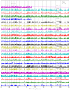 |
Fig. 2. PACS continuum subtracted spectra of our sample in the 55–75 μm range. The 12CO rotational lines are indicated by vertical dotted lines (see Table D.4). The upper-level rotational quantum number Ju of a few selected CO transitions are shown as a reference. The sources are sorted from top to bottom in these five groups: AGBs, S-type stars, extreme OH/IR stars, post-AGBs, and PNe. Within each category, targets are ordered based on the stellar effective temperature from the coolest source to the hottest one. |
The sources are sorted in Figs. 2 and 3 attending to their classification with the O-rich AGBs at the top, followed by S-type stars, OH/IR stars, post-AGB stars and PNe. Inside each group, the objects are sorted attending to the effective temperature of the central star, with the coolest object at the top and the hottest one at the bottom. The way the objects have been sorted evidences how different the spectra are along the different evolutionary stages from AGB phase to the PN stage. While the spectra of the envelopes around AGB stars show hundreds of molecular emission lines the density of emission lines in post-AGB objects is clearly lower. Finally, the most evolved objects, with highest temperatures of central stars, the PNe, show intense atomic emission lines in their envelopes and a lack of molecular features compared to the AGBs.
Rotational CO transitions in the ground vibrational state (v = 0) are the most prominent molecular lines found in all the spectra. We have detected and measured the integrated flux of CO v = 0 rotational lines with high-J levels, up to J = 42 (Eup ∼ 4700 K). We have checked that, as expected, the resolving power of PACS (of a few 100 km s−1) does not allow us to spectrally resolve the line profiles, which are expected to have full widths at half intensity similar to the terminal expansion velocity of the envelopes, FWHM ∼ 20–40 km s−1 in the majority of our sample. The PACS CO line profiles are also unresolved for a few post-AGB objects and PNs in our sample that are known to have fast outflows sampled by low-J transitions, that is OH 231.8+4.2 (Alcolea et al. 2001).
Apart from CO, we have also detected molecular emission lines from H2O, including orto- and para- configurations, OH, HCN or SiO amongst others. Some of these lines have been reported for some objects of our subsample in (e.g. Danilovich et al. 2014; Maercker et al. 2016). Atomic lines such as OI (63 μm), OIII (88 μm), NII (122 μm) and CII (158 μm) are also identified in post-AGBs and PNe, but not in AGBs. Finally, broad dust emission features associated to forsterite at 69 μm are also found in 4 objects: NGC 6537, NGC 6302, OH 231.8+4.2 and OH 26.5+0.6. Previous detections of forsterite in evolved stars with Herschel are shown, for example, in de Vries et al. (2015) and Blommaert et al. (2014). The integrated fluxes of the CO rotational emission lines detected in our sample are shown in Table D.4.
Certain CO rotational lines are known to be blended with transitions by other abundant species that lie within the same PACS spectral resolution element. We have identified, for example, the blend of CO (J = 23 − 22) with o–H2O (414–303), and that of CO(J = 22 − 21) with the 13CO(J = 23 − 22) and HNC (J = 28 − 27) transitions. Line blends were excluded in our RD analysis, but these lines are listed and integrated fluxes are reported in Table D.4 for completeness. In this table, we also list the lines that present a poor estimation of the underlying continuum level, although they have not been used for the rotational diagram analysis given their very large flux error bars. Finally, we note that the CO (J = 27 − 26) and (J = 26 − 25) transitions are missing for all targets since there is a gap in the 95–102 μm region of the PACS detector where these lines lie. The errors in the CO line fluxes are derived using the error associated to the fitting, estimated using the rms value of the continuum adjacent to the line, and assuming a flux calibration error of 15%.
In Fig. 4 we compare the integrated flux of the CO (J = 15−14) transition at 173.6 μm (FCO 15−14) with other observational parameters, in particular, with the IRAS 100 μm flux (IRAS100), the PACS continuum at 170 μm (PACS170), i.e. near the CO (J = 15−14) line, and the [12]–[25] IRAS colour. As expected, there is a correlation between the CO line strength and the IRAS100 and PACS170 continuum fluxes, which confirms that objects with stronger molecular emission show, typically, stronger continuum emission from dust as well. Of course, in addition to an intrinsic relation between these two observational parameters, there is also a dependence with the distance to the sources, which is partially responsible of the observed relation. The scatter of the points is significantly larger in the FCO 15−14 vs. IRAS100 distribution, which partially reflects the variability of the majority of the targets (pulsating AGB stars) given that PACS and IRAS observations were obtained at different epochs, as well as different instrument calibration uncertainties, background contamination sources, beam size and pointing, etc. These effects are discussed for the whole sample of the THROES catalogue in Ramos-Medina et al. (2018). We find an anticorrelation between the line-to-continuum (FCO 15−14/PACS170) ratio and the IRAS [12]–[25] colour, which are both distant-independent parameters. In general, we find that the ratio between the molecular emission and the dust emission is higher in less evolved objects than in the most evolved ones.
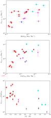 |
Fig. 4. Top: integrated flux of the CO J = 15−14 transition at 173.6 μm (FCO 15−14) against the IRAS 100 μm flux. Targets with no PACS data beyond ∼145 μm (i.e. not covering this CO transition; RR Aql and T Cep – see Fig. 3) or with bad quality (Quality Flag≠3) IRAS100 data (OH 26.5+0.6) are excluded. Middle: fluxes of the CO J = 15−14 transition and the adjacent continuum (PACS170). In this diagram, OH 26.5+0.6 is included. Bottom: line-to-continuum (F CO 15−14-to-PACS170) flux ratio against the IRAS colour [12]−[25]. |
5. CO emission analysis: rotational diagrams (RD)
The CO rotational lines provide a fundamental diagnostic of the physical conditions of the molecular gas. As a first approximation, we calculated the rotational population diagrams of the CO (Ju−J1) v = 0 transitions observed with PACS assuming optically thin emission under LTE conditions. We have used the approach presented by Justtanont et al. (2000), where the total flux observed is used to derive the total mass of the CO-emitting volume adopting the distance to the source indicated in Table D.2.
The concept of the RD analysis is very simple, see Goldsmith & Langer (1999). Assuming LTE, the population of each level Nu can be described by a single rotation temperature Trot, which is expected to be the same as the kinetic temperature, and given by the Boltzmann distribution:
 (1)
(1)
where NCO is the total number of CO molecules in the emitting volume, Q(Trot) is the rotational partition function and gu are the statistical weights for each upper level. Equation (1) can be rewritten in the following form:
 (2)
(2)
where Cτ is the opacity correction term defined as  by, e.g, Goldsmith & Langer (1999). The left hand side of Eq. (2) can be estimated using the relation between the observed flux of a single line and the number of molecules at the upper level (Nu):
 (3)
(3)
where F is the integrated line flux, λ is the rest wavelength of the transition, d is the distance to the source, Aul is the Einstein’s spontaneous emission coefficient associated to the transition, h is the Planck’s constant and c represents the speed of light.
In our RDs we represent  against
  and we apply a linear regression that allow us to obtain Trot (derived from the slope) and NCO (estimated from the intercept in the y-axis) following Eq. (2).
With the values of NCO and Trot derived from this first fitting we estimate those of τ and Cτ from Eq. (4) in Sect. 5.1. This initial estimation is used to obtain new values of  applying the correction shown in Eq. (2). Then we can apply a new linear fit to this new set of values to derive the so-called opacity corrected values for Trot and NCO that are the ones adopted for the rest of the analysis. We want to highlight that the opacity correction derived is moderate being the τ values estimated for each object close to 1 (see Sect. 5.1). Very high values of τ would lead to unreliable results from the RD analysis, see Goldsmith & Langer (1999) for details.
5.1. Opacity correction
The optical depth (τλ) of a CO line is given by:
 (4)
(4)
where  is the column density of CO in the upper level of the transition.
We need an estimation of Trot and  to calculate τ. Trot is directly extracted from the RDs and
  is derived from the total number of CO molecules, NCO, through the following, simplified, equation:
  . Where rCO represents the characteristic radius of the region where the bulk of the CO emission is produced.
The value of rCO is one of the main sources of uncertainty to compute the optical depth and the subsequent opacity correction term. Unfortunately, as mentioned in Sect. 3, the inner envelope layers where the CO PACS lines are produced are unresolved or barely resolved in the PACS spectroscopy cubes for most of the sources given the large PSF (∼9″–13″) and pixel size (9″.4) of the instrument (see Sect. 3). Therefore, the value of rCO needs to be adopted based on several criteria. These criteria are described in detail in Appendix B, and a summary is offered in the following paragraphs.
For AGB stars, an estimate of rCO is obtained by comparing the values of Trot deduced from our analysis, ∼200–700 K, with the radial temperature distribution T(r) in the envelopes of a number of AGB stars with detailed non-LTE excitation and radiative transfer studies of their CO emission. The gas temperature can be up to 2000 K near the dust condensation radius (∼1014 cm), and decreases gradually towards the outermost layers following, approximately, a power-law of the type ∼1/rα, with α ∼ 0.5−1.0, see Van de Sande et al. (2018); Maercker et al. (2016); Danilovich et al. (2014); Khouri et al. (2014). For our sample, we deduce a range of values of rCO from about 2×1014 cm to [2–4]×1015 cm, with the highest mass-loss rate objects requiring the largest values of rCO. The values of rCO adopted for our targets are given in Table D.3.
The CO column densities derived from our RD analysis adopting a range of rCO from ∼1014 to ∼1015 cm are moderate,
 < ∼ 1019cm2, resulting in line optical depths of the order of ∼0.9, and even lower in some cases, for the CO J = 14 → 13 transition, which is the line with the largest opacity in our study. For AGBs, we have tuned rCO to a value slightly larger than the radius of the wind layer where τJ = 14 → 13 ∼ 1; the latter is indeed the deepest region of the envelope observationally accessible, because of the almost null escape probability (
 ) from much deeper, optically thicker (τ ≫ 1) layers of the wind.
Not only for the AGB stars but also for the OH/IR stars, we find that values of the radius around rCO ∼ [2–4]×1015 cm result in line optical depths close to, but smaller than, unity (typically τ J = 14 → 13∼0.5–0.7) that result in moderate Cτ opacity correction factors. For all the objects studied in this work, the opacity correction is typically negligible for lines higher than J = 19−18.
Unlike for AGBs and OH/IR stars, for post-AGBs/PNe there are no theoretical or observationally constrained temperature profiles of the molecular gas component available in the literature. For these targets, we find that τJ = 14 → 13 approaches a value of ∼1 at distances of rCO ∼ 1×1016 cm, which therefore have been taken as a lower limit to the radius of the CO emitting volume detected with PACS. The PACS spectroscopy cubes indeed show extended, partially resolved nebulosities consistent with a linear diameter of ≲[1–2]×1017 cm (da Silva Santos 2016), in some of these cases. Using additional information on the molecular envelope extent from the literature and aiming to treat the sources as homogeneously as possible, we have adopted a common value of rCO = 6×1016 cm for the 5 post-AGBs/PNe in our sample, resulting in column densities of NCO ≲ 1–5×1017 cm−2 and small line optical depths of τJ = 14 → 13∼0.02–0.07.
It must be noted that, in addition, we have completed our analysis by systematically exploring a range of radii around the value of rCO adopted in each case to investigate the impact of this uncertain parameter in our results (see Fig. C.1). As expected, the smaller the rCO, the larger the opacity correction, which results in lower values of Trot and larger values of NCO. We note that after applying the Cτ correction, the slope of the RD increases, as a direct result of the frequency-dependence of Cτ and the typical values of Trot in our sample, see Appendix B. For example, in AGBs and OH/IR stars, values of rCO ≳ 5×1015 cm always result in negligible opacity corrections, whereas for values of rCO ≲ 8×1014 cm the opacity becomes larger than one for most targets, except for the sources with the lowest mass-loss rates (Ṁ ∼ 10−1 M⊙ yr−1, see Table D.2) where the CO lines remain optically thin at these radii.
6. Results
6.1. Rotational temperatures and total emitting mass of H2
The CO RDs of our targets, from which we derive the rotational temperature (Trot) and the total number of CO molecules (NCO) in the emitting volume, are shown in Figs. 5a–c. For most objects, the RDs include CO transitions with upper-level energies that range from Eup ∼ 580 K to Eup ≲ 2500 K and are well fitted using a single temperature component. The single-fit rotational temperatures obtained range from ∼200 K (NGC 6537) to ∼700 K (π Gru), with an average value of Trot ∼ 450 K.
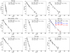 |
Fig. 5. RDs of CO for our targets (continues in 5b and 5c). For each source, the values of Trot and MH2 derived from the fits (solid lines) as well as the characteristic radius of the emitting envelope layers adopted (RCO) are shown (Sect. 5). The errors of Trot and MH2 represent the uncertainty of the fit considering the error bars of the individual points, which include formal errors due to the noise and absolute flux uncertainty of the PACS spectra. For a few sources, a double component fit was necessary. For these cases, the values of Trot and MH2 for the so-called warm (blue) and hot (red) components are also indicated. |
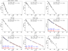 |
Fig. 5. continued. |
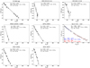 |
Fig. 5. continued. |
For a number of strong CO emitters (NML Tau, χ Cyg, W Aql, NML Cyg and IRAS 17347-3139) transitions with upper-level energies of up to Eup ∼ 5000 K are also detected. In these cases, the data points in the RD over the full Eup covered are not well reproduced by a single straight-line fit. A double-slope in the RD is expected if a range of temperatures occur along the line of sight.
We have formally tested that a double-slope fit is indeed most appropriate in these cases using statistical tools for model selection: F statistics and Bayesian Information Criterion (BIC), implemented in R programming language in the strucchange 3 package (see Paper II for more details). We refer to the CO emitting regions with the lowest and highest Trot values derived from the double-fit as the “warm” and “hot” CO components, respectively (Figs. 5a–c). The rotational temperatures of the warm and hot components are in the range ∼370–480 K and ∼570–900 K, respectively. As expected, the values of Trot obtained from a single-fit to the RDs are intermediate to those of the warm and hot components.
The total number of CO molecules in the emitting volume, NCO, derived from the RDs has been converted to total mass of molecular hydrogen using:
 (5)
(5)
where mH2 is the mass of a molecule of hydrogen (mH2 = 2.0159 a.u. = 3.3475 × 10⁻²⁴ g) and χCO is the CO-to-H2 fractional abundance, assumed to be 2 × 10⁻⁴ for O-rich objects (Ramstedt & Olofsson 2014) and 6 × 10⁻⁴ for S-type stars (Ramstedt & Olofsson 2014; Danilovich et al. 2014).
The resulting values of MH2 and Trot are listed for each target in Table D.3, together with a few other relevant parameters (such as the adopted rCO for the moderate opacity correction applied, Sect. 5.1). In Fig. 6 we show the MH2 and Trot values for each target, with and without the opacity correction, and the final histogram distributions.
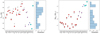 |
Fig. 6. Values of Trot and MH2 from our CO rotational diagram analysis (single fit; Sect. 6) before and after applying the opacity correction (grey and coloured symbols, respectively). |
The single-fit values of the total mass of the CO-emitting volume range between MH2 ∼ 3 × 10⁻⁶ M⊙ (X Her) and ∼5 × 10⁻² M⊙ (IRAS 17347-3139), with an average value of MH2 ∼ 4 × 10⁻³ M⊙. The opacity correction applied in all cases is small-to-moderate, which results in a mass-correction factor less than 20% in most sources. The source with the largest opacity correction (of a factor ∼1.5) is NML Cyg, the AGB star with the largest MH2, and highest mass-loss rate, in our sample (Table D.2).
The mass of the warm CO component is always larger than the mass of the hot component. For the warm component, these values vary from MH2 ∼ 1.3 × 10⁻⁵ to 7.8 × 10⁻² M⊙, and for the hot between 3.7 × 10⁻⁶ and 1.6 × 10⁻² M⊙. The warm-to-hot MH2 and Trot ratio, and their relation, is further examined in Sect. 7.
We have investigated if there are any trends between Trot and MH2, derived for our RD analysis, and other observational parameters, such as the terminal expansion velocity of the envelope (vexp) and the strength of the CO (J = 15−14) transition (Fig. 7). First, we notice that objects in the most advances stages of the evolution, namely, post-AGBs and PNe, systematically have the lowest temperatures, Trot ∼ 200–300 K, and the highest masses, MH2 > 0.01 M⊙ (see also Fig. 6). IRAS 17347-3139 is the only object with an exceptionally large Trot for its class. The distribution of Trot and MH2 for post-AGB and PNe is also much narrower than for AGBs and OH/IR. The latter show a broad range of Trot ∼ 200–700 K and MH2 ∼ 10−6 − 10−3 M⊙. This segregation of the sources exists before and after the opacity correction has been applied; the opacity correction is indeed marginal for post-AGBs and PNe (grey symbols in Fig. 6). The observed bias in favour of massive post-AGB/PNe could reflect that, in our sample, post-AGB/PNe are on average more distant (d > 1 kpc) than AGBs and OH/IRs stars, which hampers CO line detections in the less massive post-AGB/PNe.
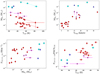 |
Fig. 7. Relation between MH2 and Trotderived from our CO RD analysis and other magnitudes. Top-left: MH2 vs. Trot. For objects (a total of five) with a double-Trot component, both the single-fit and double-fit values are connected with dashed lines for an easier identification. Top-right: values of MH2 (single-fit) vs. vexp taken from the literature. Bottom panels: integrated fluxes of CO (J = 15−14) line vs. MH2 (left) and the same line normalized to its adjacent continuum vs. Trot (right). |
We observe an anticorrelation between MH2 and Trot (Fig. 7, top-left panel). This is most clearly noticed amongst AGB and OH/IRs, which are more numerous and cover a broader range of Trot and MH2 values, but it is also followed by post-AGB/PNe. We note that for objects for which a double-Trot component has been identified (NML Tau, χ Cyg, W Aql, NML Cyg and IRAS 17347-3139), both the double- and the single-fit values (connected with dashed lines in Fig. 7, top-left panel) follow the trend. The object IRAS 17347-3139 is an outlier, since it has a much larger Trot than anticipated based on the overall properties of the rest of our sample. This object is known to be at the earliest stages of the post-AGB evolution and making a fast transition to the PN phase at present (Table D.2, see Gómez et al. 2005; Tafoya et al. 2009).
For AGBs and OH/IRs stars, there is also an evident linear correlation between MH2 and the terminal expansion velocity of the envelope (from the literature – Table D.3). As we will see in Sect. 7.4, this is linked to an analogue Ṁ-to-vexp relation, which is known to exist based on previous low-J CO studies of AGB CSEs (e.g. Danilovich et al. 2015) and that we corroborate in this work using higher-J CO lines. The post-AGB objects and PNe in our sample, however, show very similar values of the mass over a the full range of velocities.
As expected, the integrated flux of the CO lines correlate with the total mass of the CO-emitting volume and, as we will see later, with the average mass-loss rate of the envelopes. As an example we show this relation for the CO J = 15−14 transition (Eup ∼ 660 K) in Fig. 7 (bottom-left). There is a significant scatter in the line flux vs. MH2 relation since the latter also depends on the excitation temperature (Trot), the velocity field in the envelope, the optical depth, etc. (Sect. 5).
Finally, we investigated if a correlation exist between the CO J = 15−14 line integrated flux normalized to the underlying ∼170 μm-continuum observed with PACS (F CO 15−14/PACS170) and the parameters derived from the RD analysis. The strongest correlation is found with Trot (Fig. 7, bottom-right), which is somewhat expected since the mass and the distance dependence is removed in the line-to-continuum flux ratio. The relation between F CO 15−14/PACS170 with MH2 (not shown) has a much larger scatter and suggests a certain anticorrelation (given that Trot anticorrelates with MH2 in our sample).
In Sect. 7 we further discuss the observed trends.
6.2. Mass-loss rate
Using the values of the total emitting mass, we calculate the mass-loss rates (Ṁ) for each source in a simplified manner dividing the total mass by the crossing time of the CO-emitting layers, that is:
 (6)
(6)
Apart from MH2, derived from the RDs, we need to adopt a value for the expansion velocity (vexp), which has been taken from literature, as well as for the characteristic radius of the CO emitting region, for which we use the same value used for the estimation of the opacity correction, rCO. The values of Ṁ are given in Table D.2.
In Sect. 5, we already mentioned the uncertainties associated to the adoption of a particular linear radius for the emitting region of each source and the importance of exploring a wide range of values to determine a reasonable estimation of the opacity correction and, thus, of MH2. The same kind of analysis is even more important now, as the impact of rCO in the mass-loss rate estimation is larger than in the calculation of the opacity correction (it affects MH2 but also directly Ṁ as ∼ 1/rCO). Another uncertainty arises in vexp, however, this parameter is rather well known (from previous works), to an accuracy of ∼10–20% typically.
In Fig. C.2, we show, for every object, the different values of Ṁ and Trot that correspond to three different values of the radius around the adopted value. For each source, we have also plotted a grey region that represents the broad interval of mass-loss rates found in the literature. The latter are usually derived from the analysis of low-J CO lines and, therefore, they represent the average mass-loss rate in the outer envelope layers. These values of Ṁ from the literature have been re-scaled after matching the expansion velocity (vexp), the distance (d) and the relative abundance of CO ( χ CO) to the values adopted here, which is needed for a proper comparison with our estimates of Ṁ. The values of the mass-loss rates reported in the bibliography for each object are displayed in Table D.2 together with the associated interval range of mass-loss rates after scaling and relevant references. To our knowledge, for IRAS 17347-3139 and NGC 6537 there are no previous estimates of the gas mass-loss rate in the literature.
Our estimates of the mass-loss rates are shown in Fig. 8 plotted against the rotational temperature, the expansion velocity, and the CO (J = 15−14) line strength to explore any trends that may be present. In the Ṁ vs. Trot diagram we also include the mass-loss rates associated to the warm and hot component for objects with a double-slope in their RDs. There is an anti-correlation between Ṁ and Trot, which was expected based on a similar trend observed directly between MH2 and Trot (Fig. 7). This trend together with the clear correlation between Ṁ and vexp and, more scattered, trend with FCO 15−14 are briefly discussed in Sect. 7.
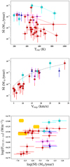 |
Fig. 8. Top: relation between Ṁ and Trot. Single- and double-fit (warm and hot) values, whenever these exist, are connected using dashed lines. Middle: relation between Ṁ and vexp. The distribution approaches a power-law of the type Ṁ ∝ vexp2.5 (dashed line). Bottom: integrated flux of the CO J = 15−14 line vs. Ṁ in a logarithmic scale. |
7. Analysis and interpretation of the results
In this section, we analyse and discuss the results obtained from the RDs as well as the correlations found between different magnitudes.
7.1. Rotational temperature and total mass
For most of our sources, a single-Trot component was sufficient to obtain a good fit of the CO RD, leading to single-fit rotational temperatures and total (H2) masses of the CO-emitting region of Trot ∼ 200–700 K and MH2 ∼3 × 10⁻⁶ − 5 × 10⁻² M⊙, respectively (Sect. 6).
The rotational temperatures of a few 100 K derived in this work using CO-PACS data (Ju ∼ 14–27, and up to Ju = 40 lines in some cases) are clearly larger than the typical values of Trot ∼ 10–100 K found from CO low-J line studies (most commonly using Ju < 4 lines at mm and sub-mm wavelengths) in the external layers of the CSE around evolved stars, at ≈1016 − 1017 cm from the center (e.g. Teyssier et al. 2006, and references therein). This corroborates that, as anticipated, the CO-PACS lines sample the warm, presumably inner, regions of the CSEs, probably at a typical/average distance from the central star of about ≈1015 cm for AGB stars (e.g. Danilovich et al. 2014).
We find that the total mass of the warm inner layers where the PACS CO (Ju > 14) lines mainly arise is typically a factor ∼100–1000 lower than the masses deduced from low-J CO line studies in the literature, reinforcing the idea that CO PACS lines sample mainly the inner part of the envelopes, which contains a small fraction of the total envelope mass.
For a total of five targets in our sample (NML Tau, π Gru, W Aql, χ Cyg and IRAS 17347-3139), the RD diagram shows a double slope and, thus, a double-Trot fit is most appropriate. Deviations from a single straight line fit of the RDs, most likely denoting a temperature stratification along the line of sight (see below), are not uncommon and have been previously found in a number of AGB and post-AGB CSEs using ISO and/or SPIRE CO spectra (e.g. Justtanont et al. 2000; Wesson et al. 2010; Matsuura et al. 2014; Cernicharo et al. 2015; Cordiner et al. 2016).
The rotational temperatures and masses of the hot and warm components of these five objects are displayed in Fig. 7 (together with the single-fit Trot and MH2 values derived for the whole sample). The mass of the warm component is always larger (by a factor 2–10) than that of the hot component. Adopting a constant mass-loss rate and a gas temperature that decreases with the distance, the difference between the mass of the warm and hot component suggests a CO-emitting volume smaller for the hot component than for the warm one.
We compare in detail the hot-to-warm MH2 and Trot ratios in Fig. 9. We find that the mass and temperature ratios are well correlated and follow approximately a power-law function. For AGB CSE with an inverse-square density profile, the latter is indeed expected if the temperature stratification within the emitting layers is described by a power-law function, T(r)∼1/rα. This is because, in this case, the total mass within a given CO-emitting volume is roughly proportional to its radius (MH2 ∝ r) and, therefore, it is easy to derive that:
 (7)
(7)
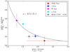 |
Fig. 9. Ratio of the mass and rotational temperatures for the hot and warm components, |
Fitting a power-law function to the set of points corresponding to our AGB stars4, we obtain α = 0.5 ± 0.1. This value is at the low end of the range of exponents found in the literature (from a combination of theoretical modelling and observational works) for AGB CSEs, typically α ∼ 0.5 − 1 (e.g. De Beck et al. 2010; Maercker et al. 2016; Danilovich et al. 2015, and references therein). There is some indication from recent works that the kinetic temperature distribution is shallower, with values of α down to ∼0.4, for the inner CSE layers (∼5×10¹⁴–3×1015 cm; De Beck et al. 2012; Lombaert et al. 2016) than for the outer regions, where the steepest temperature variations (α∼1–1.2) are found (≳1016 cm; Teyssier et al. 2006). This is indeed in very good agreement with the small value of α found in the inner envelope layers from our analysis. (The hot-to-warm mass vs. Trot trend with a similar value of α is also deduced in our sample of C-rich targets studied in Paper II). We believe that the empirical relation between the hot-to-warm ratio of MH2 and Trot therefore supports that the double-Trot component identified in some of our objects (and possibly also present in more targets for which CO Ju > 27 transitions remain undetected), is a natural consequence of the temperature stratification across the inner envelope layers. Detailed non-LTE excitation and radiative transfer of the CO emission including high-J transitions, Ju ∼ 14–40, are needed for a proper characteriztion of the temperature structure in the warm inner-wind regions of AGB stars. See Appendix A for a discussion of non-LTE effects on the RD analysis.
7.2. Comparison with other works: ṀTHROES vs. ṀBibliography
In Fig. 10 we show, for each source, the mass-loss rate estimated in this work for the adopted radius (rCO) against a mean value of gas mass-loss rates found in the bibliography (ṀBibliography). We assign error bars of a factor 3 to our estimates of the mass-loss rate; this is a common uncertainty value adopted in most molecular line-emission studies (e.g. Maercker et al. 2016). The error bars of ṀBibliography represent the low and high ends of the broad range of values found in bibliography after scaling to our d, vexp and χCO values, and is always ∼3 or more. For objects with only one value of Ṁ from the literature, an uncertainty factor of 3 has also been assumed after scaling.
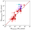 |
Fig. 10. Comparison of the mass-loss rates from this work and from the literature (Tables D.2 and D.3, respectively). The solid line represents a 1:1 ratio. Target colour and symbol code as in Fig. 1. The big circles are used to locate a few targets with previous ṀBibliography estimates obtained from non-LTE excitation and radiative transfer analysis of CO lines, including some of the PACS transitions. |
The comparison between our mass-loss rates and those found in the bibliography is in quite good agreement for all the objects, see also Fig. C.2. As already mentioned, we are particularly interested in the comparison of our Ṁ with those obtained from comprehensive non-LTE excitation and radiative transfer models that make use of some CO rotational lines (normally, J < 20) measured with PACS, which exist for a small sample of objects: for R Cas, NML Tau, TX Cam, R Dor, W Hya and W Aql (Van de Sande et al. 2018; Maercker et al. 2016; Khouri et al. 2014; Danilovich et al. 2014). We find that, also in these cases, discrepancies with our values are always within 50% for all sources except W Hya, demonstrating that the simple and approximate RD approach and the assumptions (e.g. the adopted size of the emitting layers) used in this work yield reasonable first estimate results.
Considering again our sample as a whole, our mass-loss rate estimations of post-AGBs and PNe seem to be systematically lower than those in the literature by a ∼20%. In principle, this small difference could suggest that the radius of the CO-emitting region is slightly smaller than the value of rCO adopted by us (at least in some objects). As it is shown in Fig. C.2, a fine tuning of rCO can be performed to obtain a perfect match between ṀBibliography and our estimates for each individual object. However, we prefer to treat the sources as homogeneously as possible and to be conservative avoiding the use of very small values of rCO, which would result in large opacities ( τ ≫ 1) and would consequently lead to unreliable opacity corrections.
A similar discrepancy is reported by Danilovich et al. (2015) from a CO-line study (including non-LTE radiative transfer modelling) of AGB CSEs in the SUCCESS programme including CO transitions from J = 1 − 0 to J = 9 − 8, as well as J = 14 − 13 in some targets. Their models give mass-loss rates that are on average 40% lower than those derived from past studies (see their Fig. 7). Danilovich et al. (2015) note that, as already mentioned here, most past studies are based on observations of a small number of low-J CO transitions (with similar excitation conditions, i.e., Eup), and conclude that taking a large sample of CO transitions, including high-J lines, properly into account when modelling mass-loss rates, results in lower derived values.
It is important to stress that the mass-loss rates derived in this work represent average values during the period of time when the warm, inner envelope layers were ejected, that is, during the last < 50–100 years, for AGBs, and the last ∼600–2000 years, for PNe (considering the values of rCO and vexp given in Table D.3). Since the low-J lines commonly used in the previous studies to derive ṀBibliography mainly trace the outer envelope layers, the discrepancies observed with respect to past studies could reflect a real time variation of the mass-loss rate in some cases. This is indeed the case of OH 231.8+4.2, where mass-loss rate when the bulk of the nebula was ejected during the last ≈1000 yr (∼2×10⁻⁴ M⊙, Alcolea et al. 2001) is much larger than the present-day mass-loss rate (< 2×10⁻⁵ M⊙), Sánchez Contreras et al. 2002). The upper limit to the present-day mass-loss rate of OH 231.8+4.2 is indeed in very good agreement with our estimate using high-J CO transitions.
Finally, as a word of caution we note that the mass-loss rates estimated for post-AGB objects and PNs are particularly uncertain as it is not easy to define essential parameters like rCO or vexp for these spatio-kinematically and morphologically complex objects. This makes the comparison with values from past studies subject to larger uncertainties. In spite of this, the agreement is reasonably good for the two post-AGBs and one PN in our sample with values of Ṁ reported in the literature.
7.3. Mass and mass-loss rate vs. Trot
As shown in Fig. 7, we find a statistically significant anticorrelation between the total mass of the PACS-CO emitting region, MH2, and the rotational temperature, Trot, derived from our RD analysis. As expected, a similar trend is present between the mass-loss rate, Ṁ, and Trot (Fig. 8).
Prior to this work, Teyssier et al. (2006) and Danilovich et al. (2015) noticed a tentative Ṁ vs. Trot anticorrelation based on their studies of the intermediate-to-outer regions of the envelopes of AGB and post-AGB stars using submm/mm-wavelength CO transitions. Particularly, Danilovich et al. (2015) reported Ṁ and Tkin at a representative distance of ≈1016 cm (i.e. ∼100 times the dust condensation radius) for a sample of 53 AGB stars. From their analysis, using self-consistent non-LTE radiative transfer models of the dust continuum emission and the CO emission transitions over a range of excitations (from J = 1 − 0 to J = 9 − 8, and in a few cases, up to J = 14 − 13), Danilovich et al. (2015) found that in general high mass-loss rate objects show relatively low temperatures (see their Fig. 6).
The temperatures of the regions studied by Danilovich et al. (2015), at distances ∼[1–2]×1016 cm, range between ∼10 and 80 K to be compared with the larger temperatures, ∼200–600 K, found by us at distances typically a factor ∼10 smaller in our AGB+OH/IR targets. This indicates that this trend is preserved from the inner envelope layers, traced by Ju ≥ 14 CO lines, through the outer parts of the CSE, sampled by lower-J transitions.
As discussed by Danilovich et al. (2015), a possible reason for the anticorrelation observed is the more efficient line cooling expected for high mass-loss rate objects (see also Groenewegen 1994, and references therein). In addition to this, we believe that optical depth effects can partially contribute to, and reinforce, the observed anticorrelation. This is because for high mass-loss rate objects, the τ CO∼1 surface layer, which is the deepest region that can be observationally sampled by a given CO line, is located at larger distances from the star where the gas kinetic temperature is lower.
7.4. Mass and mass-loss vs. expansion velocities
In Sect. 6 we already mentioned the presence of evident correlations between MH2 and vexp and between Ṁ and vexp (Figs. 7 and 8, respectively).
The correlation found between MH2 and vexp is stronger if we consider only the AGB and OH/IR stars in our sample. In AGB and OH/IRs stars, the observed correlation could be telling us about the processes which are responsible for the acceleration of the stellar wind. Since AGB winds are primarily driven by radiation pressure on dust, the most luminous objects (which are also the most massive) will exhibit the largest expansion velocities.
The fact that post-AGB and PNs deviate from the observed trend is probably related with the different mass-loss mechanism (not driven by radiation pressure on dust) in these latest stages (Bujarrabal et al. 2001).
Moreover, the expansion velocities of post-AGBs and PNs do not represent the terminal velocity of the present-day stellar wind but the result from the complex hydrodynamical interaction between the stellar high-velocity winds, that appear beyond the AGB phase, and the slow ambient circumstellar material (expelled in the previous AGB stage).
Based on the above conclusion that, in AGB stars, vexp correlates with MH2 via the stellar luminosity, the trend found between vexp and Ṁ is not surprising (Fig. 8). In this case, however, the post-AGBs and PNs in our sample do not deviate significantly from the general trend, although, as we mentioned above, the values and interpretation of vexp as well as the Ṁ derived (under simplifying assumptions) have to be regarded with caution.
The Ṁ-to-vexp relation has been observed before in other CO line studies in AGB CSEs. For example, Danilovich et al. (2015) report a correlation between Ṁ and vexp, including stars of different chemical types (O-rich, C-rich and S-stars), which is in very good agreement with our data-points (in spite of the lower-J transitions, J < 14, used by these authors). We have fitted a power-law function to the observed distribution (dashed line in Fig. 8-middle panel), the best fit gives an index of about 3 (i.e., Ṁ ∝vexp2.5 ) although the uncertainties associated to the fitting are important (2.5 ± 1).
7.5. Other trends
As shown in Sect. 6, we find a clear and expected correlation between the strength of the CO line emission, in particular, of the J = 15−14 line (F CO 15−14), with MH2 and Ṁ (Figs. 7 and 8, respectively). The correlation found by us is in very good agreement with that reported recently by Lombaert et al. (2016) using a number of CO transitions observed with PACS to model the envelopes of a sample of C-rich AGB CSEs with H2O emission. The dependence with the distance to the sources of F CO 15−14, MH2 and Ṁ partially explain the observed trend; additionally, the line flux is proportional to the amount of mass in the emitting volume (Eq. (3)), although other factors, such as the opacity and the excitation temperature, have an important influence.
The influence of the excitation temperature in the resulting strength of the CO lines relative to the continuum becomes evident in Fig. 8-bottom panel, where we see a clear correlation between FCO 15−14/PACS170 and Trot, which are both distance independent parameters. We find that objects with the lowest values of Trot show small line-to-continuum (FCO 15−14/PACS170) ratios. We have found from this work that post-AGBs and PNs have the most massive envelopes in our sample (> 0.01–0.1 M⊙), but in spite of this, they are relatively weak high-J CO emitters as a consequence of the relatively low excitation conditions prevailing in their envelopes (Trot ∼ 200–300 K). Other factors, such as a different gas-to-dust mass fraction at different evolutionary stages, may also lie behind the observed trend.
8. Summary
We have analysed Herschel-PACS 1D spectra of 26 evolved low-to-intermediate mass stars, in different evolutionary stages from the AGB to the PN phase, contained in the THROES catalogue5. Our sample includes 23 O-rich and 3 S-type objects (C-rich targets are separately studied in Paper II).
RDs using high-excitation CO v = 0 rotational emission lines, with upper-level energies Eup ∼ 580–5000 K, have been created to study the warm inner layers of the CSEs of these objects. We derive fundamental physical parameters such as: rotational temperatures (Trot), total molecular mass in the CO-emitting layers (MH2) and average mass-loss rates during the ejection of these layers (Ṁ).
The rotational temperatures are found to vary from ∼200 K to ∼700 K. For AGB and OH/IR stars, which represent ∼80% of our sample, the rotational temperatures are around Trot ∼ 500 K and systematically larger than for the most evolved objects, post-AGBs and PNs (Trot ∼ 200 K). These temperatures are one order of magnitude higher than estimated from past low-J CO line studies of the outer envelope. This is expected as, in the PACS far-infrared range, we are tracing gas that is closer to the central star (≈1015 cm for AGBs and ≈1016 cm for post-AGBs and PNs).
The total mass of the inner CSE regions where the PACS CO lines arise ranges from MH2 ∼ 10−6 to 10−2M⊙ in our sample, with the most evolved objects being the most massive. The values of MH2 found in this work are typically 100–1000 times lower than the total envelope mass obtained from previous low-J CO line studies.
The mass-loss rates estimated are in the range Ṁ ≈ 10−7 − 10−4 M⊙ yr−1, in agreement (within uncertainties) with values found in the literature.
For some strong CO emitters in our sample (NML Tau, χ Cyg, W Aql, NML Cyg and IRAS 17347−3139) a double temperature (hot and warm) component is inferred. The temperatures of the warm and hot components are ∼400–500 K and ∼600–900 K, respectively. The mass of the warm component (∼10−5 − 8 × 10⁻² M⊙) is always larger than that of the hot component, by a factor ∼2–10.
The warm-to-hot MH2 and Trot ratios in our sample are correlated and are consistent with an average temperature radial profile of ∝ r−0.5 ± 0.1, that is, slightly shallower than in the outer envelope layers, in agreement with recent studies.
We have explored the distributions of the different magnitudes and physical parameters of these objects and if any trends exist. We find that MH2 and Ṁ are both anticorrelated with Trot. This is interpreted as a combination of two different processes: CO line cooling and opacity effects. Previous works have also reported similar trends based on low-J CO line observations.
A strong correlation has been found, also, between MH2 and vexp, particularly for AGB stars. This correlation is also present in the Ṁ vs. vexp distribution, as expected. This trend, which is observed in past studies using low-J CO transitions, is consistent with the wind acceleration mechanism being more efficient in the more luminous and massive stars.
Although IRAS 17347-3139 does not deviate significantly from the observed hot-to-warm MH2 vs. Trot trend, we excluded this object from the fit because, being a young PNe, it does not necessarily follows the same density and temperature profiles of the AGB CSEs.
Also available from the Leiden Lambda Database web page.
Acknowledgments
We acknowledge support from the Faculty of the European Space Astronomy Centre (ESAC). C.S.C. acknowledges financial support by the Spanish MINECO through grants AYA2016-75066-C2-1-P and by the European Research Council through ERC grant 610256: NANOCOSMOS. We also acknowledge our referee, Kay Justtanont, for her useful and precise comments which have helped to improve our work.
References
- Alcolea, J., Bujarrabal, V., Sánchez Contreras, C., Neri, R., & Zweigle, J. 2001, A&A, 373, 932 [NASA ADS] [CrossRef] [EDP Sciences] [Google Scholar]
- Balick, B., & Frank, A. 2002, ARA&A, 40, 439 [NASA ADS] [CrossRef] [Google Scholar]
- Blommaert, J. A. D. L., de Vries, B. L., Waters, L. B. F. M., et al. 2014, A&A, 565, A109 [NASA ADS] [CrossRef] [EDP Sciences] [Google Scholar]
- Bocchio, M., Bianchi, S., & Abergel, A. 2016, A&A, 591, A117 [NASA ADS] [CrossRef] [EDP Sciences] [Google Scholar]
- Bowen, G. H. 1988, ApJ, 329, 299 [NASA ADS] [CrossRef] [Google Scholar]
- Bujarrabal, V. 1999, in Asymptotic Giant Branch Stars, eds. T. Le Bertre, A. Lebre, & C. Waelkens, IAU Symp., 191, 363 [Google Scholar]
- Bujarrabal, V., Castro-Carrizo, A., Alcolea, J., & Sánchez Contreras, C. 2001, A&A, 377, 868 [NASA ADS] [CrossRef] [EDP Sciences] [Google Scholar]
- Cernicharo, J., Teyssier, D., Quintana-Lacaci, G., et al. 2014, ApJ, 796, L21 [NASA ADS] [CrossRef] [Google Scholar]
- Cernicharo, J., McCarthy, M. C., Gottlieb, C. A., et al. 2015, ApJ, 806, L3 [NASA ADS] [CrossRef] [Google Scholar]
- Choi, Y. K., Brunthaler, A., Menten, K. M., & Reid, M. J. 1999, in Cosmic Masers - from OH to H0, eds. R. S. Booth, W. H. T. Vlemmings, & E. M. L. Humphreys, IAU Symp., 287, 407 [NASA ADS] [CrossRef] [Google Scholar]
- Cordiner, M. A., Boogert, A. C. A., Charnley, S. B., et al. 2016, ApJ, 828, 51 [NASA ADS] [CrossRef] [Google Scholar]
- Cox, N. L. J., Kerschbaum, F., van Marle, A.-J., et al. 2012, A&A, 537, A35 [NASA ADS] [CrossRef] [EDP Sciences] [Google Scholar]
- Danilovich, T., Bergman, P., Justtanont, K., et al. 2014, A&A, 569, A76 [NASA ADS] [CrossRef] [EDP Sciences] [Google Scholar]
- Danilovich, T., Teyssier, D., Justtanont, K., et al. 2015, A&A, 581, A60 [NASA ADS] [CrossRef] [EDP Sciences] [Google Scholar]
- da Silva Santos, J. M. 2016, Master’s Thesis, University of Porto, Portugal [Google Scholar]
- De Beck, E., Decin, L., de Koter, A., et al. 2010, A&A, 523, A18 [NASA ADS] [CrossRef] [EDP Sciences] [Google Scholar]
- De Beck, E., Lombaert, R., Agúndez, M., et al. 2012, A&A, 539, A108 [NASA ADS] [CrossRef] [EDP Sciences] [Google Scholar]
- Decin, L. 2012, Adv. Space Res., 50, 843 [NASA ADS] [CrossRef] [Google Scholar]
- Decin, L., Hony, S., de Koter, A., et al. 2007, A&A, 475, 233 [NASA ADS] [CrossRef] [EDP Sciences] [Google Scholar]
- Decin, L., Justtanont, K., De Beck, E., et al. 2010, A&A, 521, L4 [Google Scholar]
- de Vries, B. L., Maaskant, K. M., Min, M., et al. 2015, A&A, 576, A98 [NASA ADS] [CrossRef] [EDP Sciences] [Google Scholar]
- Dinh-V-Trung, Bujarrabal, V., Castro-Carrizo, A., Lim, J., & Kwok, S. 2008, ApJ, 673, 934 [NASA ADS] [CrossRef] [Google Scholar]
- Doan, L., Ramstedt, S., Vlemmings, W. H. T., et al. 2017, A&A, 605, A28 [NASA ADS] [CrossRef] [EDP Sciences] [Google Scholar]
- Goldsmith, P. F., & Langer, W. D. 1999, ApJ, 517, 209 [NASA ADS] [CrossRef] [Google Scholar]
- Gómez, J. F., de Gregorio-Monsalvo, I., Lovell, J. E. J., et al. 2005, MNRAS, 364, 738 [NASA ADS] [CrossRef] [Google Scholar]
- Groenewegen, M. A. T. 1994, A&A, 290, 531 [NASA ADS] [Google Scholar]
- Groenewegen, M. A. T., Waelkens, C., Barlow, M. J., et al. 2011, A&A, 526, A162 [NASA ADS] [CrossRef] [EDP Sciences] [Google Scholar]
- Habing, H. J. 1996, A&ARv, 7, 97 [NASA ADS] [CrossRef] [Google Scholar]
- He, J. H., Szczerba, R., Hasegawa, T. I., & Schmidt, M. R. 2014, ApJS, 210, 26 [NASA ADS] [CrossRef] [Google Scholar]
- He, J. H., Dinh-V-Trung, J. H., & Hasegawa, T. I. 2017, ApJ, 845, 38 [NASA ADS] [CrossRef] [Google Scholar]
- Heras, A. M., & Hony, S. 2005, A&A, 439, 171 [NASA ADS] [CrossRef] [EDP Sciences] [Google Scholar]
- Herwig, F. 2005, ARA&A, 43, 435 [NASA ADS] [CrossRef] [Google Scholar]
- Höfner, S., & Olofsson, H. 2018, A&ARv, 26, 1 [NASA ADS] [CrossRef] [Google Scholar]
- Justtanont, K., Barlow, M. J., Tielens, A. G. G. M., et al. 2000, A&A, 360, 1117 [NASA ADS] [Google Scholar]
- Justtanont, K., Decin, L., Schöier, F. L., et al. 2010, A&A, 521, L6 [NASA ADS] [CrossRef] [EDP Sciences] [Google Scholar]
- Justtanont, K., Teyssier, D., Barlow, M. J., et al. 2013, A&A, 556, A101 [NASA ADS] [CrossRef] [EDP Sciences] [Google Scholar]
- Karakas, A. I., van Raai, M. A., Lugaro, M., Sterling, N. C., & Dinerstein, H. L. 2009, ApJ, 690, 1130 [NASA ADS] [CrossRef] [Google Scholar]
- Khouri, T., de Koter, A., Decin, L., et al. 2014, A&A, 561, A5 [NASA ADS] [CrossRef] [EDP Sciences] [Google Scholar]
- Knapp, G. R., Phillips, T. G., Leighton, R. B., et al. 1982, ApJ, 252, 616 [NASA ADS] [CrossRef] [Google Scholar]
- Kwok, S. 2005, J. Korean Astron. Soc., 38, 271 [NASA ADS] [CrossRef] [Google Scholar]
- Lombaert, R., Decin, L., Royer, P., et al. 2016, A&A, 588, A124 [NASA ADS] [CrossRef] [EDP Sciences] [Google Scholar]
- Loup, C., Forveille, T., Omont, A., & Paul, J. F. 1993, A&AS, 99, 291 [NASA ADS] [Google Scholar]
- Maercker, M., Schöier, F. L., Olofsson, H., Bergman, P., & Ramstedt, S. 2008, A&A, 479, 779 [NASA ADS] [CrossRef] [EDP Sciences] [Google Scholar]
- Maercker, M., Danilovich, T., Olofsson, H., et al. 2016, A&A, 591, A44 [Google Scholar]
- Marigo, P., Bernard-Salas, J., Pottasch, S. R., Tielens, A. G. G. M., & Wesselius, P. R. 2003, A&A, 409, 619 [NASA ADS] [CrossRef] [EDP Sciences] [Google Scholar]
- Matsuura, M., Zijlstra, A. A., Gray, M. D., Molster, F. J., & Waters, L. B. F. M. 2005, MNRAS, 363, 628 [NASA ADS] [Google Scholar]
- Matsuura, M., Yates, J. A., Barlow, M. J., et al. 2014, MNRAS, 437, 532 [NASA ADS] [CrossRef] [Google Scholar]
- Meaburn, J., Lloyd, M., Vaytet, N. M. H., & López, J. A. 2008, MNRAS, 385, 269 [NASA ADS] [CrossRef] [Google Scholar]
- Millar, T. J. 2016, J. Phys. Conf. Ser., 728, 052001 [CrossRef] [Google Scholar]
- Nhung, P. T., Hoai, D. T., Winters, J. M., et al. 2015, A&A, 583, A64 [NASA ADS] [CrossRef] [EDP Sciences] [Google Scholar]
- Olofsson, H., González Delgado, D., Kerschbaum, F., & Schöier, F. L. 2002, A&A, 391, 1053 [NASA ADS] [CrossRef] [EDP Sciences] [Google Scholar]
- Pilbratt, G. L., Riedinger, J. R., Passvogel, T., et al. 2010, A&A, 518, L1 [CrossRef] [EDP Sciences] [Google Scholar]
- Poglitsch, A., Waelkens, C., Geis, N., et al. 2010, A&A, 518, L2 [NASA ADS] [CrossRef] [EDP Sciences] [Google Scholar]
- Ramos-Medina, J., Sánchez Contreras, C., García-Lario, P., et al. 2018, A&A, 611, A41 [NASA ADS] [CrossRef] [EDP Sciences] [Google Scholar]
- Ramstedt, S., & Olofsson, H. 2014, A&A, 566, A145 [NASA ADS] [CrossRef] [EDP Sciences] [Google Scholar]
- Ramstedt, S., Schöier, F. L., Olofsson, H., & Lundgren, A. A. 2006, A&A, 454, L103 [NASA ADS] [CrossRef] [EDP Sciences] [Google Scholar]
- Ramstedt, S., Schöier, F. L., Olofsson, H., & Lundgren, A. A. 2008, A&A, 487, 645 [NASA ADS] [CrossRef] [EDP Sciences] [Google Scholar]
- Ramstedt, S., Schöier, F. L., & Olofsson, H. 2009, A&A, 499, 515 [NASA ADS] [CrossRef] [EDP Sciences] [Google Scholar]
- Sánchez Contreras, C., & Sahai, R. 2012, ApJS, 203, 16 [NASA ADS] [CrossRef] [Google Scholar]
- Sánchez Contreras, C., Desmurs, J. F., Bujarrabal, V., Alcolea, J., & Colomer, F. 2002, A&A, 385, L1 [NASA ADS] [CrossRef] [EDP Sciences] [Google Scholar]
- Sánchez Contreras, C., Velilla Prieto, L., Agúndez, M., et al. 2015, A&A, 577, A52 [NASA ADS] [CrossRef] [EDP Sciences] [Google Scholar]
- Santander-García, M., Bujarrabal, V., Koning, N., & Steffen, W. 2015, A&A, 573, A56 [NASA ADS] [CrossRef] [EDP Sciences] [Google Scholar]
- Schöier, F. L., & Olofsson, H. 2001, A&A, 368, 969 [NASA ADS] [CrossRef] [EDP Sciences] [Google Scholar]
- Schöier, F. L., Maercker, M., Justtanont, K., et al. 2011, A&A, 530, A83 [NASA ADS] [CrossRef] [EDP Sciences] [Google Scholar]
- Simis, Y. J. W., Icke, V., & Dominik, C. 2001, A&A, 371, 205 [NASA ADS] [CrossRef] [EDP Sciences] [Google Scholar]
- Tafoya, D., Gómez, Y., Patel, N. A., et al. 2009, ApJ, 691, 611 [NASA ADS] [CrossRef] [Google Scholar]
- Teyssier, D., Hernandez, R., Bujarrabal, V., Yoshida, H., & Phillips, T. G. 2006, A&A, 450, 167 [NASA ADS] [CrossRef] [EDP Sciences] [Google Scholar]
- Teyssier, D., Cernicharo, J., Quintana-Lacaci, G., et al. 2015, in Why Galaxies Care about AGB Stars III: A Closer Look in Space and Time, eds. F. Kerschbaum, R. F. Wing, & J. Hron, ASP Conf. Ser., 497, 43 [Google Scholar]
- Ueta, T., Ladjal, D., Exter, K. M., et al. 2014, A&A, 565, A36 [NASA ADS] [CrossRef] [EDP Sciences] [Google Scholar]
- van der Veen, W. E. C. J., & Habing, H. J. 1988, A&A, 194, 125 [NASA ADS] [Google Scholar]
- Van de Sande, M., Decin, L., Lombaert, R., et al. 2018, A&A, 609, A63 [NASA ADS] [CrossRef] [EDP Sciences] [Google Scholar]
- Vickers, S. B., Frew, D. J., Parker, Q. A., & Bojičić, I. S. 2015, MNRAS, 447, 1673 [NASA ADS] [CrossRef] [EDP Sciences] [Google Scholar]
- Wesson, R., Cernicharo, J., Barlow, M. J., et al. 2010, A&A, 518, L144 [NASA ADS] [CrossRef] [EDP Sciences] [Google Scholar]
- Woods, P. M., Nyman, L.-Å., Schöier, F. L., et al. 2005, A&A, 429, 977 [NASA ADS] [CrossRef] [EDP Sciences] [MathSciNet] [Google Scholar]
- Yang, B., Stancil, P. C., Balakrishnan, N., & Forrey, R. C. 2010, ApJ, 718, 1062 [NASA ADS] [CrossRef] [Google Scholar]
Appendix A: Non-LTE effects
The rotational diagram (RD) method is a classical and widely used line-emission analysis technique useful to obtain a first estimate of the excitation temperature and mass of the gas in the line emitting region (Goldsmith & Langer 1999; Justtanont et al. 2000). As explained in Sect. 5, it is based on two major assumptions: optically thin emission and excitation under LTE conditions. A canonical opacity correction factor, Cτ, has been included to take into account moderate optical depth effects (Sect. 5). Here, we examine whether non-LTE excitation effects are expected to be significant in our sample and, if this is the case, what is the impact on the values of MH2 and Trot inferred from our RD analysis. We present several arguments that suggest that although small LTE deviations cannot be ruled out (particularly, in the lowest mass-loss rate objects), we expect a negligible impact on the derived values of MH2. Additionally, the double slope in the RD observed for some targets predominantly reflects the temperature stratification in the emitting layers.
A first simple evaluation of LTE deviations is obtained from the comparison of the critical densities of the CO transtions studied here and the densities expected in the CO-emitting regions in our sample. For most (80%) of our targets, the far-IR CO transitions detected and used in our RD analysis arise from states ∼500–2000 K above the ground, i.e. with upper-level rotational quantum numbers Ju ∼ 14–27. According to most recent collisional rate coefficients computed by Yang et al. (2010)6, these transitions have critical densities of ncrit ∼ 5×10⁵ and 3×106 cm−3, for Ju = 14 and Ju = 27, respectively, for a range of temperatures consistent with our estimates, ∼200 and 700 K, see Fig. 10 in Yang et al. (2010).
From the lowest to the highest mass-loss rate objects in our sample (Ṁ ∼ 2×10⁻⁷–1×10⁻⁴ M⊙ yr−1, Fig. 8), densities of nH2 ≳106 − 108 cm−3 are expected at the typical radius adopted (from rCO ∼ 4×10¹⁴ to rCO ∼ [1–4]×1015 cm, respectively – see Table D.2, Appendix B) consistent with CO population levels predominantly thermalized in most cases.
As already pointed out in pioneering studies of ISO-LWS observations of high-J CO lines using the RD approach, see Justtanont et al. 2000, the mere fact that we detect CO Ju ∼ 14–27 transitions together with a roughly linear distribution in the RD is a hint of high-density gas and level populations in this range of Ju close to thermal equilibrium.
For a few targets, we also detect CO lines with upper-levels above Ju > 27, which have critical densities of ncrit ∼ 106 − 107 cm−3 and, therefore, some LTE deviations cannot be rule out (but we note that these transitions presumably arise from regions closer to the center, within the dust formation layers).
The simple calculations above are indeed corroborated by non-LTE excitation and radiative transfer analysis computations of a selection of high-J CO transitions observed with PACS (from Ju = 14 to 38) on a sample of C-rich AGB CSEs by Lombaert et al. (2016). These authors conclude that over the broad range of mass-loss rates studied in their work, Ṁ ∼ 10−7–2×10⁻⁵ M⊙ yr−1, which is comparable to the range in our sample, the CO molecule is predominantly excited through collisions with H2, with a minor effect of far-IR radiative pumping due to the dust radiation field.
We stress that even under non-LTE conditions, for a simple diatomic molecule like CO, the RD method provides a reliable measure of the total mass within the emitting volume. This is because, although Trot may deviate from the kinetic temperature, Tkin, in regions where the local density is lower than the critical densities of the transitions considered, it does describe quite precisely the molecular excitation (i.e. the real level population). To test this idea and to check the reliability of our analysis, we have compared our values of MH2 and Ṁ with those obtained from state-of-the-art line excitation and radiative transfer models of high-J CO transitions, sometimes including PACS data, performed by other authors in objects of our sample. To our knowledge, these have been published for a total of 6 sources: R Cas, R Dor, TX Cam, NML Tau, W Hya and W Aql (see Van de Sande et al. 2018; Maercker et al. 2016; Danilovich et al. 2014; Khouri et al. 2014 and references therein). For these objects, the CO emission over a broad range of Eup has been modelled to derive the temperature, density and velocity profile across their ∼1014 − 1017 cm CSE layers, as well as the mass-loss rate of the stellar wind. As shown in Sect. 6, discrepancies between our values of Ṁ and those obtained from comprehensive non-LTE radiative transfer analysis are very small, always within 50%, demonstrating that the simple and approximate RD approach and the assumptions (e.g. the adopted size of the emitting layers) used in this work yield reasonable results.
An additional test of the reliability and uncertainties of the RD method is presented in Paper II, where we perform our RD analysis using multi-epoch CO-PACS spectra for the C-rich AGB star IRC+10216. This object shows prominent line variability (mainly of high-excitation transitions of CO and other molecules) denoting radiative farIR (ro-vibrational) pumping via the dust radiation field modulated by the stellar pulsation (Cernicharo et al. 2014; Teyssier et al. 2015; He et al. 2017). This object, thus, serves as a benchmark for testing the effect of radiative vs. collisional excitation and its impact of the values of MH2 and Trot derived from our RD analysis. We corroborate that, in spite of strong CO line flux variations and confirmed changes in the relative level population, the total number of emitting molecules (adding up all levels) from the RD analysis remains constant (within uncertainties, < 15%) at multiple epochs. This is true for both the warm and hot components (both identified in IRC+10216) and, thus, for the single-fit value of MH2.
We also find that line variability has also a small impact on the value of Trot derived at multiple epochs in IRC+10216. The values of Trot from the single-fit and warm component (using Ju < 27 transitions) remain essentially constant within uncertainties, consistent with negligible impact of non-LTE effects (if any). The highest-excitation CO lines (Ju > 27) show stronger variations and, as a consequence, the variations of Trot for the hot component are larger, of ≲±15% about the average, maybe denoting some repercussion of LTE deviations on Trot in this case.
Although it is improbable given our previous discussion, let us now consider whether the double slope in the RD diagram found for a few objects in our sample could predominantly result from non-LTE effects, with Trot deviating most significantly from Tkin for the highest-J CO transitions, and what would be the implications in this case.
Among our targets (O-rich and S-type), we find a double-Trot component in a total of five sources, covering a broad range of mass-loss rates, from Ṁ ∼ 2×10⁻⁷ to 8×10⁻⁵ M⊙ yr−1. The mass-loss rate distribution of these sources is the same as the sources for which only one Trot component is found. Moreover, we do not find any correlation between Ṁ and the properties of the hot and warm components (also including C-rich targets, see e.g. Fig. A.1), which makes improbable the double Trot component being predominantly a non-LTE effect (expected to be most remarkable in low mass-loss rate objects).
Moreover, to explain the observed double slope as a purely non-LTE effect, two conditions need to be simultaneously met in all double-Trot targets. First, a very specific value of the number density, in a narrow range around ∼107 cm−3, is needed to have Ju < 27 levels close to thermal equilibrium but Ju > 27 levels deviating perceivably from LTE (this would generate the double slope in the RD diagram). Second, a strong background radiation source Tbg > Tkin is required to reproduce a Trot that is higher for Ju > 27 transitions than for Ju < 27 lines. Dust mixed with the gas in the CO-emitting volume and heated by the stellar radiation to 800 K could produce the required Tbg. If this is the case, then it would also imply similarly high gas temperatures in the emitting region since the difference between the gas and dust temperature across these inner wind layers is expected to be moderate (of < 100 K) and to follow a similar radial dependence based on detailed dust-continuum and non-LTE radiative transfer CO emission models (e.g. for W Aql, Tkin ∼ Tdust ∼ 300 K at rCO = 2×1015 cm Danilovich et al. 2014). In the extreme case (e.g. maybe for very low mass-loss rate objects with densities < 106 cm−3) that Trot is totally decoupled from Tkin but very close to Tbg for all transitions from Ju = 14 to 40, then the double-slope of the RDs would most likely reflect the stratification of the dust temperature (rather than the gas) across the envelopes.
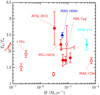 |
Fig. A.1. Ratio of the hot-to-warm rotational temperature vs. the mass-loss rates for objects with a double-Trot component: targets from this work (Paper I) are represented by open symbols, C-rich objects (from Paper II) are plotted using filled symbols. |
Summarizing, a minor impact of small LTE deviations on the values of MH2 and Ṁ is expected, even for the targets with the lowest mass-loss rates, Ṁ ≈ 10−7 M⊙ yr−1. The double slope of the RD is unlikely to be primarily due to large LTE deviations and points to a temperature stratification in the warm inner layers of the envelopes probed by PACS CO line emission. The temperature profile deduced is further discussed in Sect. 7.1.
Appendix B: The characteristic radius of the CO-emitting volume
In this appendix, we provide a more detailed description of the procedure that we have followed to decide on a “characteristic” radius of the CO-emitting volume (rCO) to be used to compute, and correct for, the CO line opacities (Sect. 5.1) and to obtain an estimate of the mean mass-loss rate of our targets (Sect. 6.2).
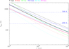 |
Fig. B.1. Power-law radial distribution of the gas kinetic temperature estimated from non-LTE excitation and radiative transfer models of the CO emission in a number of AGB envelopes (indicated at the top of the box using the same colour for the temperature laws) from the literature. References: Van de Sande et al. (2018); Maercker et al. (2016); Khouri et al. (2014); Decin et al. (2010). The solid and dotted lines of R Dor and IK Tau are different temperature profiles derived by different authors (solid from Maercker et al. 2016, and dotted from Van de Sande et al. 2018 – R Dor and Decin et al. 2010 – IK Tau). The thick black line is an average temperature law. |
For AGB CSEs (also including OH/IRs), a first estimate of the size of the CO-emitting volume is derived using the envelope temperature structure estimated from detailed non-LTE excitation and radiative tranfer calculations in the literature. These exist for many AGB CSEs using low-J CO transitions (typically Ju ≲ 6), and, for more reduced samples, also using certain CO transitions from higher J levels.
In Fig. B.1 we show temperature power-law radial profiles in the form
 that have been deduced in a number of previous works (references are given in the figure caption) for the few targets in our sample that include at least one high-J CO line observed with any of the three Herschel instruments (HIFI, SPIRE, or PACS). As we see in this figure, the full range of rotation temperatures deduced from our RD analysis, Trot ∼ 200–700 K (Sect. 6), is consistent with the bulk of the PACS CO emission studied here arising from layers between ∼2×10¹⁴ and ∼5×1015 cm, if we take together all the T(r) distributions in Fig. B.1 (coloured lines), or between ∼3×10¹⁴ and ∼3×1015 cm, if we use an average T(r) power-law (thick black line, in Fig. B.1). The quadratic mean of these two ranges is rCO ∼ 1015 cm, which we uniformly use as the reference value in most AGB stars to compute MH2, Trot, and Ṁ (but see more details below). Since the radius is, in any case, uncertain, we offer additional estimates of these parameters for a larger range of radius around the default rCO (Appendix C). As we will see next, for the lowest (larger) mass-loss rate AGB stars in our sample, the characteristic CO-radius could be a factor of ∼2–4 smaller (larger) than the rCO ∼ 1015 cm reference value.
In the following, we perform a case-by-case RD analyis of three targets (R Dor, W Aql, and TX Cam) that are representative of three main mass-loss regimes in our sample: low, medium and high (Ṁ ≈ M⊙ yr−1, ≈10−6 M⊙ yr−1, and ≳10−5 M⊙ yr−1, respectively) and for which detailed non-LTE excitation and radiative transfer studies of the CO emission including some mid-to-high Ju-CO transitions exist in the literature. The purpose is twofold: (1) to better illustrate our method to constrain rCO in our sample (needed to decide on a plausible reference value for a uniform analysis), and (2) to compare the mass-loss rates from our approximate RD analysis with those computed using more sophisticated modelling tools.
R Dor. Precise CO-modelling studies of the molecular envelope of this object, including CO transitions up to Ju = 16 (Eup = 750 K), have been carried out by Maercker et al. (2016) and Van de Sande et al. (2018), references to other molecular line studies using lower-Ju transitions are given in Table D.2;); . The gas temperature structure deduced from these works, which use the same set of CO lines, are not fully coincident (dotted and solid red lines in Fig. B.1). Van de Sande et al. (2018) claim that their model achieves a better fit to more lines, and therefore, we adopt the T(r) power-law determined by these authors, with an exponent α = 0.65.
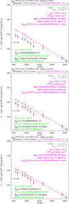 |
Fig. B.2. Rotational diagrams of the low mass-loss rate O-rich AGB star R Dor to illustrate the different steps that we have routinely followed to constrain rCO according to our temperature-opacity combined criteria (full details are given in the text, Appendix B). |
Our general procedure to determine an optimal/acceptable value of rCO is as follows. From a linear fit to the CO datapoints in the RD diagram (dotted line and black dots, respectively, in the top panel of Fig. B.2) we find a first or iteration-zero estimate of Trot(i = 0) before any opacity correction is applied. Assuming that Trot(i = 0) ∼ 570 K represents (or is close to) the average gas temperature within the CO-emitting volume and using the T(r) function depicted in Fig. B.1, we derive an initial value of rCO(i = 0) ∼ 2.5×1014 cm. We use this radius to compute the opacity of the different transitions. In this case, we obtain τ14 → 13∼1.8 for the CO J = 14 − 13 line, and smaller for higher-J lines (see Eq. (4)). After applying the opacity correction, through the frequency-dependent factor Cτ = τ/(1 − −e−τ), a second linear fit to the opacity-corrected datapoints is performed (pink line and dots, respectively, in top panel of Fig. B.2), resulting in a new estimate of Trot(i = 1). The latter always is smaller than the iteration-zero value because after applying the Cτ correction, the slope of the RD increases, as a direct result of the frequency-dependence of Cτ and the typical values of Trot that we measure in our sample. Comparing again the value of Trot(i = 1) ∼ 480 K with the T(r) law, we deduce a new value of rCO(i = 1) ∼ 3.4×1014 cm, where the gas would have such a temperature.
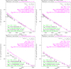 |
Fig. B.3. Rotational diagram of W Aql and NML Tau (bottom). Left: results of the RD for rCO = 1×1015 cm, which results in a perfect match between the opacity- and temperature-radius (labelled as rCO and rT, respectively, in the plot) but results in an undesired large opacity correction, τ14 → 13> 1. Right: results of the RD for rCO = 1.4×1015 cm, which satisfies our τ14 → 13 < 1 criteria. |
This exercise indicates that an intermediate value between rCO(i = 0) and rCO(i = 1) is needed to reach full consistency between the rCO value used for the opacity correction and the one that reproduces the opacity-corrected Trot derived (according to the T(r) adopted). In the particular case of R Dor, we find a perfect match between rCO(i = 0) and rCO(i = 1) for rCO ∼ 3.15×1014 cm (leading to Trot(i = 1) ∼ 500 K at this radius – Fig. B.1, middle panel).
An additional constrain to the radius is obtained from the fact that, as already explained in Sect. 5, the deepest layer traced by the observed CO emission must be such that τ< 1. In order to satisfy this moderate-opacity condition, a value of rCO slightly larger than the “perfect-match” rCO above is preferred. For R Dor, a value of rCO ∼ 3.5×1014 cm satisfies the opacity criteria (τ14 → 13< 1) and is, within uncertainties, still fully consistent with the radius where the final value of Trot is attained, adopting the T(r) law from previous works – Fig. B.2, bottom panel). The mass-loss rate that results adopting this value of the radius rCO ∼ 3.5×1014 cm, which guarantees line opacities lower than 1, is Ṁ ∼ 4×10⁻⁷ M⊙ yr−1.
In this and in most targets, in principle we cannot rule out a larger radius (leading to even lower line opacities), even if Trot deviates from the gas temperature predicted at that radius based on the T(r) law adopted. This is because there is no guarantee that the adopted T(r) is a 100% accurate representation of the real temperature structure in these inner-wind regions and because Trot may not be either a 100% accurate representation of the temperature of the gas (especially for low mass-loss rate objects). For R Dor, if we adopt the default radius of rCO ∼ 1×1015 cm previously established as a reasonable characteristic radius for the overall AGB class, we deduce a temperature of Trot ∼ 570 K and a mass-loss rate of Ṁ ∼ 1×10⁻⁷ M⊙ yr−1.
For R Dor, the mass-loss rates derived from Van de Sande et al. (2018) and Maercker et al. (2016) from their non-LTE CO excitation and radiative transfer analysis are very similar in both cases (∼2×10⁻⁷ M⊙ yr−1) and lie within the range of values estimated by us from our simple RD approach and the plausible range of rCO explored, Ṁ ∼ [1–4]×10−7 M⊙ yr−1.
W Aql. Non-LTE excitation and radiative transfer of the CO emission, including CO transitions up to Ju = 25 (Eup = 1796 K), have been carried out for this S-type AGB star by Danilovich et al. (2014). The mass-loss rate obtained in this work is Ṁ ∼ 4×10⁻⁶ M⊙ yr−1 (as quoted in Table D.2, where we provide additional references to other molecular line studies using lower-Ju transitions). Danilovich et al. (2014) derive the gas and dust temperature profile in the 2×10¹⁴–1017 cm envelope layers (see their Fig. 3). Both the gas and dust temperatures are quite similar throughout the whole envelope, with the dust being slighly cooler than the gas below 2×1015 cm (i.e. the region sampled by the PACS CO data). In this region, the gas and dust temperatures do not differ by more than 50% (in particular, at ∼1015 cm, values of Tdust∼ 400 K and Tkin ∼ 500 K are expected).
In Fig. B.1 we reproduce the gas temperature structure deduced by Danilovich et al. (2014); the exponent of this power-law function is α = 0.65. We have used this profile to constrain rCO following the same procedure explained in the previous paragraphs for R Dor. As we can see in the left panel of Fig. B.3, a radius of rCO ∼ 1×1015 cm produces a perfect match between the final (opacity-corrected) temperature derived (Trot ∼ 500 K) and the radius where this temperature is expected (rT) according to Danilovich et al. (2014). This value of the radius, however, results in line opacities larger than desirable and a mass-loss rate of Ṁ ∼ 9×10⁻⁶ M⊙ yr−1. In this case, the radius that produces τ14 → 13< 1 and simultaneously satisfies (within uncertainties) the temperature criteria is rCO ∼ 1.4×1015 cm (right panel of Fig. B.3. This results in a somewhat smaller mass-loss rate of Ṁ ∼ 5×10⁻⁶ M⊙ yr−1, which is in excellent agreement with previous estimates.
IK Tau. The physical properties of the circumstellar gas, including the temperature, velocity and density structure, have been determined from the radiative transfer modelling of the multi-transitional (sub)millimetre CO line observations by Decin et al. (2010) and Maercker et al. (2016). The temperature distributions from these two works differ substantially (as for R Dor) and are shown in Fig. B.1 (solid and dotted cyan lines).
Adopting the α = 0.6 distribution derived by Decin et al. (2010), we find that a radius of rCO ∼ 5×1014 cm produces a perfect match between the final (opacity-corrected) value of the temperature (Trot = 420 K) and the radius rT where this temperature is expected, however, it results in opaque lines (Fig. B.3, bottom-left). For IK Tau, a radius of rCO ∼ 9×1014 cm or larger is needed to meet the τ14 → 13< 1 criteria (Fig. B.3, bottom-rigth). This results in a somewhat smaller mass-loss rate of Ṁ ∼ 1×10⁻⁵ M⊙ yr−1, also in agreement with the range of values from previous estimates (Ṁ ∼ [0.2–3.5]×10−5 M⊙ yr−1, Table D.2).
Rest of the targets. We have followed this procedure to constrain the range of rCO values that are plausible (based on our opacity- and temperature- combined criteria) for each target individually. Whenever a T(r) distribution was available in the literature (this happened for a few targets, see Fig. B.1) we used that specific law, and for the rest we used a mean T(r) distribution represented by the thick black line in Fig. B.1 as a guide.
Remarks on the temperature profiles. The T(r) profiles used and represented in Fig. B.1, although obtained from detailed non-LTE excitation and radiatiave transfer models of the CO emission, are not free from large uncertainties. This is denoted by the discrepancies between the temperature structure derived for the same targets when computed by different teams (notable cases are R Dor and IK Tau, in spite of these being among the most studied and best characterized AGB envelopes). Moreover, the power-law distribution is only an approximation to the real temperature structure. Indeed, the latter can deviate significantly from a simple power-law in some regions, in particular, T(r) can have multiple-slopes as well as local minima and maxima as shown in De Beck et al. (De Beck et al. (2010), see their Fig. 9, )) and (Maercker et al. (2016), see their Fig. 5,)).
Additionally, given the moderate range of Ju in the CO transitions predominantly modelled and published to date, the curves represented in Fig. B.1 are expected to be most reliable in the intermediate-to-outer envelope layers, beyond ∼1015 cm. Recently, Lombaert et al. (2016) performed non-LTE excitation and radiative transfer models of a sample of C-rich AGB CSEs using a selection of seven high-J CO transitions observed with PACS and SPIRE covering levels from Ju = 15 to 38, that is, higher than in the studies represented in Fig. B.1. One interesting result from this study is that the temperature of the gas falls off less steeply, with a power-law exponent close to α ∼ 0.4 − 0.5, in the inner-warm envelope regions sampled by these high-J CO transitions. This is indeed consistent with the crude estimate of α deduced in this work by comparing the hot and warm envelope components for a few targets in our sample (see Sect. 7). More dedicated non-LTE excitation and radiative transfer models of the high-J CO emission in larger samples is needed to confirm this result and to obtain a more precise description of the temperature distribution in these inner and warm regions of the envelopes of AGB stars.
Final remark on the reference values of rCO. It is evident that the value of rCO derived using a temperature criteria is very model-dependent since it fully relies on T(r) and on Trot being a perfect representation of Tkin. For this reason, we prefer to be cautious and, after having explored carefully the range of plausible rCO values based on a temperature-opacity combined criteria for all targets, to use a set of (order-of-magnitude) estimates of rCO for the whole sample, rather than using the best-match radius individually found for each target. As shown in Table D.2, we chose a reference radius: rCO = 1×1015 cm for most AGB CSEs, rCO = [2–4]×1015 cm for high-Ṁ AGB CSEs (> 1×10⁻⁵ M⊙ yr−1) and rCO = [4–6]×1014 cm for low-Ṁ AGB CSEs (< 1×10⁻⁶ M⊙ yr−1).
As discussed in Sect. 5, the temperature profile in the molecular envelopes of post-AGB objects and PN is extremely poorly characterized due to a much more limited number of CO emission cartography and, most importantly, modelling studies (especially using high-J CO transitions). Based on the systematically low values of Trot in post-AGB objects and PNs found in this work (∼200 K) as well as their generally larger dimensions, we chose a reference value of the radius of rCO = 6×1016 cm in these cases (Table D.3), although we explored a larger range of rCO (examples are given in Figs. C.1 and C.2). This range of rCO resulted in negligible RD opacity corrections in all these sources.
Appendix C: Additional opacity and mass-loss rate plots
In this appendix we show, for each source, the values of the optical depth (τ, defined in Sect. 5.1) of the different CO transitions used to build the RDs for a range of values of the characteristic radius (rCO) of the CO-emitting volume (Fig. C.1). As we can see in this figure, the radius adopted implies a moderate value of τ and, therefore, a moderate opacity correction. The radius of the PACS CO-emitting region is the major source of uncertainty in the computation of τ and, therefore, of the emitting mass and mass-loss rates. It also has an effect on the rotational temperature. The values of MH2 and Trot for a range of rCO are plotted inside the boxes in Fig. C.1. The resulting mass-loss rates, Ṁ, are shown in Fig. C.2, together with the broad range of mass-loss rates found in the literature for each object, typically derived from low-J CO line studies (references are provided in Table D.2).
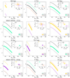 |
Fig. C.1. Plots of τ vs. Eup corresponding to different linear radii. In each chart there is a subgraphic showing MH2 vs. Trot. The thickest curve and the biggest point are those associated to the rCO shown in Table D.3. |
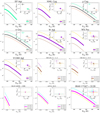 |
Fig. C.1. continued. |
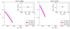 |
Fig. C.1. continued. |
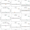 |
Fig. C.2. Plots of Ṁ vs. Trot. In each panel three different points, corresponding to three different rCO are shown. The point of the rCO shown in Table D.3 is bigger than the rest. The grey region represents the interval of mass-loss rates covered by previous works found in bibliography. For more details see Sect. 6. The linear radii explored are the same as the ones shown in Fig. C.1. |
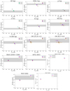 |
Fig. C.2. continued. |
Appendix D: Tables
Observations log.
Stellar and circumstellar information taken from the bibliography for the objects of the sample.
Results from our CO RD analysis (Sect. 6), including double-fit (hot and warm) components for NML Tau, χ Cyg, π Gru, W Aql, and IRAS 17347-3139.
Integrated fluxes of 12CO lines for 26 sources studied in this work.
All Tables
Stellar and circumstellar information taken from the bibliography for the objects of the sample.
Results from our CO RD analysis (Sect. 6), including double-fit (hot and warm) components for NML Tau, χ Cyg, π Gru, W Aql, and IRAS 17347-3139.
All Figures
|
Fig. 1. IRAS colour–colour diagram (left) and 100 μm flux vs. [12]−[25] IRAS colour (right) of the THROES targets with good quality IRAS data (Quality Flag = 3) in the 12, 25, 60 and 100 μm bands. The colour–colour diagram is divided in different boxes where sources with common characteristics and evolutionary stages are located (see van der Veen & Habing 1988, for details). Objects with CO line detections, studied in this work, are highlighted using the symbol and colour code shown in the figure. In the rest of the plots presented throughout this paper, AGBs, OH/IRs, post-AGBs and PNe are coloured and symbol-coded as indicated in this figure. |
| In the text | |
|
Fig. 2. PACS continuum subtracted spectra of our sample in the 55–75 μm range. The 12CO rotational lines are indicated by vertical dotted lines (see Table D.4). The upper-level rotational quantum number Ju of a few selected CO transitions are shown as a reference. The sources are sorted from top to bottom in these five groups: AGBs, S-type stars, extreme OH/IR stars, post-AGBs, and PNe. Within each category, targets are ordered based on the stellar effective temperature from the coolest source to the hottest one. |
| In the text | |
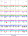 |
Fig. 3. The same as in Fig. 2 but covering the spectral range from 110 to 190 μm. |
| In the text | |
|
Fig. 4. Top: integrated flux of the CO J = 15−14 transition at 173.6 μm (FCO 15−14) against the IRAS 100 μm flux. Targets with no PACS data beyond ∼145 μm (i.e. not covering this CO transition; RR Aql and T Cep – see Fig. 3) or with bad quality (Quality Flag≠3) IRAS100 data (OH 26.5+0.6) are excluded. Middle: fluxes of the CO J = 15−14 transition and the adjacent continuum (PACS170). In this diagram, OH 26.5+0.6 is included. Bottom: line-to-continuum (F CO 15−14-to-PACS170) flux ratio against the IRAS colour [12]−[25]. |
| In the text | |
|
Fig. 5. RDs of CO for our targets (continues in 5b and 5c). For each source, the values of Trot and MH2 derived from the fits (solid lines) as well as the characteristic radius of the emitting envelope layers adopted (RCO) are shown (Sect. 5). The errors of Trot and MH2 represent the uncertainty of the fit considering the error bars of the individual points, which include formal errors due to the noise and absolute flux uncertainty of the PACS spectra. For a few sources, a double component fit was necessary. For these cases, the values of Trot and MH2 for the so-called warm (blue) and hot (red) components are also indicated. |
| In the text | |
|
Fig. 5. continued. |
| In the text | |
|
Fig. 5. continued. |
| In the text | |
|
Fig. 6. Values of Trot and MH2 from our CO rotational diagram analysis (single fit; Sect. 6) before and after applying the opacity correction (grey and coloured symbols, respectively). |
| In the text | |
|
Fig. 7. Relation between MH2 and Trotderived from our CO RD analysis and other magnitudes. Top-left: MH2 vs. Trot. For objects (a total of five) with a double-Trot component, both the single-fit and double-fit values are connected with dashed lines for an easier identification. Top-right: values of MH2 (single-fit) vs. vexp taken from the literature. Bottom panels: integrated fluxes of CO (J = 15−14) line vs. MH2 (left) and the same line normalized to its adjacent continuum vs. Trot (right). |
| In the text | |
|
Fig. 8. Top: relation between Ṁ and Trot. Single- and double-fit (warm and hot) values, whenever these exist, are connected using dashed lines. Middle: relation between Ṁ and vexp. The distribution approaches a power-law of the type Ṁ ∝ vexp2.5 (dashed line). Bottom: integrated flux of the CO J = 15−14 line vs. Ṁ in a logarithmic scale. |
| In the text | |
|
Fig. 9. Ratio of the mass and rotational temperatures for the hot and warm components, |
| In the text | |
|
Fig. 10. Comparison of the mass-loss rates from this work and from the literature (Tables D.2 and D.3, respectively). The solid line represents a 1:1 ratio. Target colour and symbol code as in Fig. 1. The big circles are used to locate a few targets with previous ṀBibliography estimates obtained from non-LTE excitation and radiative transfer analysis of CO lines, including some of the PACS transitions. |
| In the text | |
|
Fig. A.1. Ratio of the hot-to-warm rotational temperature vs. the mass-loss rates for objects with a double-Trot component: targets from this work (Paper I) are represented by open symbols, C-rich objects (from Paper II) are plotted using filled symbols. |
| In the text | |
|
Fig. B.1. Power-law radial distribution of the gas kinetic temperature estimated from non-LTE excitation and radiative transfer models of the CO emission in a number of AGB envelopes (indicated at the top of the box using the same colour for the temperature laws) from the literature. References: Van de Sande et al. (2018); Maercker et al. (2016); Khouri et al. (2014); Decin et al. (2010). The solid and dotted lines of R Dor and IK Tau are different temperature profiles derived by different authors (solid from Maercker et al. 2016, and dotted from Van de Sande et al. 2018 – R Dor and Decin et al. 2010 – IK Tau). The thick black line is an average temperature law. |
| In the text | |
|
Fig. B.2. Rotational diagrams of the low mass-loss rate O-rich AGB star R Dor to illustrate the different steps that we have routinely followed to constrain rCO according to our temperature-opacity combined criteria (full details are given in the text, Appendix B). |
| In the text | |
|
Fig. B.3. Rotational diagram of W Aql and NML Tau (bottom). Left: results of the RD for rCO = 1×1015 cm, which results in a perfect match between the opacity- and temperature-radius (labelled as rCO and rT, respectively, in the plot) but results in an undesired large opacity correction, τ14 → 13> 1. Right: results of the RD for rCO = 1.4×1015 cm, which satisfies our τ14 → 13 < 1 criteria. |
| In the text | |
|
Fig. C.1. Plots of τ vs. Eup corresponding to different linear radii. In each chart there is a subgraphic showing MH2 vs. Trot. The thickest curve and the biggest point are those associated to the rCO shown in Table D.3. |
| In the text | |
|
Fig. C.1. continued. |
| In the text | |
|
Fig. C.1. continued. |
| In the text | |
|
Fig. C.2. Plots of Ṁ vs. Trot. In each panel three different points, corresponding to three different rCO are shown. The point of the rCO shown in Table D.3 is bigger than the rest. The grey region represents the interval of mass-loss rates covered by previous works found in bibliography. For more details see Sect. 6. The linear radii explored are the same as the ones shown in Fig. C.1. |
| In the text | |
|
Fig. C.2. continued. |
| In the text | |
Current usage metrics show cumulative count of Article Views (full-text article views including HTML views, PDF and ePub downloads, according to the available data) and Abstracts Views on Vision4Press platform.
Data correspond to usage on the plateform after 2015. The current usage metrics is available 48-96 hours after online publication and is updated daily on week days.
Initial download of the metrics may take a while.