| Issue |
A&A
Volume 618, October 2018
|
|
|---|---|---|
| Article Number | A16 | |
| Number of page(s) | 21 | |
| Section | Stellar atmospheres | |
| DOI | https://doi.org/10.1051/0004-6361/201832852 | |
| Published online | 05 October 2018 | |
3D non-LTE corrections for Li abundance and 6Li/7Li isotopic ratio in solar-type stars⋆
I. Application to HD 207129 and HD 95456
1 Leibniz-Institut für Astrophysik Potsdam, An der Sternwarte 16, 14482 Potsdam, Germany
e-mail: This email address is being protected from spambots. You need JavaScript enabled to view it.
2 GEPI, Observatoire de Paris, PSL Research University, CNRS, Univ. Paris Diderot, Sorbonne Paris Cité, Place Jules Janssen, 92190 Meudon, France
3 Instituto de Astrofísica de Canarias, 38200 La Laguna, Tenerife, Spain
Received:
19
February
2018
Accepted:
29
June
2019
Abstract
Context. Convective motions in solar-type stellar atmospheres induce Doppler shifts that affect the strengths and shapes of spectral absorption lines and create slightly asymmetric line profiles. One-dimensional (1D) local thermodynamic equilibrium (LTE) studies of elemental abundances are not able to reproduce this phenomenon, which becomes particularly important when modeling the impact of isotopic fine structure, like the subtle depression created by the 6Li isotope on the red wing of the Li I resonance doublet line.
Aims. The purpose of this work is to provide corrections for the lithium abundance, A(Li), and the 6Li/7Li isotopic ratio that can easily be applied to correct 1D LTE lithium abundances in G and F dwarf stars of approximately solar mass and metallicity for three-dimensional (3D) and non-LTE (NLTE) effects.
Methods. The corrections for A(Li) and 6Li/7Li are computed using grids of 3D NLTE and 1D LTE synthetic lithium line profiles, generated from 3D hydro-dynamical CO5BOLD and 1D hydrostatic model atmospheres, respectively. For comparative purposes, all calculations are performed for three different line lists representing the Li I λ670.8 nm spectral region. The 3D NLTE corrections are then approximated by analytical expressions as a function of the stellar parameters (Teff, log ℊ, [Fe/H], ν sin i, A(Li), 6Li/7Li). These are applied to adjust the 1D LTE isotopic lithium abundances in two solar-type stars, HD 207129 and HD 95456, for which high-quality HARPS observations are available.
Results. The derived 3D NLTE corrections range between −0.01 and +0.11 dex for A(Li), and between −4.9 and −0.4% for 6Li/7Li, depending on the adopted stellar parameters. We confirm that the inferred 6Li abundance depends critically on the strength of the Si I 670.8025 nm line. Our findings show a general consistency with recent works on lithium abundance corrections. After the application of such corrections, we do not find a significant amount of 6Li in any of the two target stars.
Conclusions. In the case of 6Li/7Li, our corrections are always negative, showing that 1D LTE analysis can significantly overestimate the presence of 6Li (up to 4.9% points) in the atmospheres of solar-like dwarf stars. These results emphasize the importance of reliable 3D model atmospheres combined with NLTE line formation for deriving precise isotopic lithium abundances. Although 3D NLTE spectral synthesis implies an extensive computational effort, the results can be made accessible with parametric tools like the ones presented in this work.
Key words: stars: abundances / stars: atmospheres / radiative transfer / line: formation / line: profiles
The table with the 3D NLTE corrections is only available at the CDS via anonymous ftp to cdsarc.u-strasbg.fr (130.79.128.5) or via http://cdsweb.u-strasbg.fr/cgi-bin/qcat?J/A+A/618/A16
© ESO 2018
1. Introduction
The lithium abundance, A(Li)1, and the 6Li/7Li isotopic ratio measured in stellar atmospheres can provide valuable information contributing to understanding different problems in astrophysics such as stellar structure and evolution, stellar activity, exoplanetary system evolution and even cosmology. A reliable determination of the lithium content in stellar atmospheres is important, and apart from requiring high-resolution stellar spectra with high signal-to-noise ratios (S/Ns), it also requires realistic stellar atmosphere models allowing a sound theoretical interpretation of both the strength and the shape of the Li lines.
The stable isotope 7Li is among the few light elements that have been produced in the Big Bang. In contrast, the other stable isotope, 6Li, is not produced in significant amounts in standard Big Bang nucleosynthesis (e.g., Thomas et al. 1993), but mainly through spallation and α + α fusion reactions triggered by high-energy collisions between Galactic cosmic rays and He, C, N, O nuclei in the interstellar medium (e.g., Meneguzzi et al. 1971; Prantzos et al. 1993; Prantzos 2012). Additional 7Li is produced by the same mechanism, and partly by stellar nucleosynthesis as well. The current 6Li/7Li in the local interstellar medium (ISM) is measured to be ∼13% (Kawanomoto et al. 2009, see also Howk et al. 2012), while the solar system (meteoritic) 6Li/7Li is 8.2% (Lodders 2003).
Both 6Li and 7Li are very fragile with respect to nuclear reactions with protons and are destroyed in stellar interiors at temperatures above ∼2.0 × 10⁶ K and ∼2.5 × 10⁶ K, respectively (e.g., Pinsonneault 1997). According to standard stellar evolution models, 6Li, being the more fragile of the two isotopes, undergoes an intense destruction during pre-main sequence evolution (e.g., Forestini 1994; Proffitt & Michaud 1989; Montalbán & Rebolo 2002). The standard models predict that by the time a solar-type solar-metallicity star reaches the main sequence its 6Li has already been destroyed by nuclear reactions at the base of the extended, completely mixed convective envelope. In non-standard stellar evolution, where additional processes such as rotational mixing, atomic diffusion, internal gravity waves, and the effect of magnetic fields are included in order to explain the observed lithium abundances in stellar atmospheres (see Talon & Charbonnel 2005 and references therein), lithium destruction is generally even enhanced compared to the standard models.
This suggests that any significant detection of the fragile 6Li isotope in the atmosphere of a solar-type star would most probably indicate an external pollution process, for example by planetary matter accretion (Israelian et al. 2001) or alternative sources like stellar flares (Montes & Ramsey 1998). 6Li can also be produced by superflares around stars with hot Jupiters (Cuntz et al. 2000). Therefore, it is of great interest to measure the presence of the 6Li isotope in solar-type stars with effective temperatures between 5900 and 6400 K (see Montalbán & Rebolo 2002) and, in case of a positive detection, to investigate its origin.
Israelian et al. (2001) measured 6Li/7Li in the giant-planet hosting star HD 82943 and found a significant amount of 6Li in its atmosphere (6Li/7Li = 12%, reduced to 5% after being remeasured by Israelian et al. 2003). This finding was interpreted as evidence for a planetary material accretion on the surface of the star. 6Li/7Li has been measured afterwards by several other groups in small samples of main-sequence solar-metallicity stars with and without known planets (Reddy et al. 2002; Mandell et al. 2004; Ghezzi et al. 2009; Pavlenko et al. 2018), but no significant detections of 6Li have been reported.
The use of one-dimensional (1D) model atmospheres can lead to erroneous results in terms of lithium isotopic ratios, due to the fact that the missing convective line asymmetry must be compensated by a spurious 6Li abundance to fit the observed line profile. The result is an overestimation of 6Li/7Li using 1D model atmospheres (e.g., Cayrel et al. 2007, Steffen et al. 2012). Furthermore, not only Li but also all other spectral lines have asymmetric profiles. The asymmetry depends on several factors such as the mean depth of formation and atomic mass. The use of detailed three-dimensional (3D) hydrodynamical model atmospheres allows us to obtain more reliable abundances and isotopic ratios, in particular since they are able to treat the convective motions responsible for the line asymmetries in a much more realistic way compared to standard 1D model atmospheres. In addition, in the case of lithium, the line formation must be treated considering departures from local thermodynamic equilibrium (LTE) that are known to be significant, especially in metal-poor stars (Cayrel et al. 2007), affecting not only the strength of the spectral line but also its Doppler shift.
On the other hand, 3D non-LTE (NLTE) calculations are computationally demanding and not easily accessible to the scientific community. For this reason, it is important to provide some simplified approach to correct the results of any 1D LTE spectral analysis of the lithium line region for both 3D and NLTE effects. Such an approach was suggested by Steffen et al. (2010a,b, 2012). In Steffen et al. (2012), the authors used a grid of 3D model atmospheres to derive a polynomial approximation for deriving the 3D NLTE correction of 6Li/7Li as a function of Teff, log ℊ and metallicity ([Fe/H] from −3 to 0).
A similar approach was followed by Sbordone et al. (2010) for the lithium abundance. They derived analytical approximations to convert the equivalent widths (EW) of the lithium 670.8 nm line into A(Li) (and vice versa) in 1D LTE, 1D NLTE and 3D NLTE, which, in principle, can be used to infer the 3D NLTE abundance correction by comparing the 1D LTE and 3D NLTE A(Li) for a given EW, Teff, log ℊ and [Fe/H].
Several authors have previously performed 1D NLTE analyses of A(Li), covering a large range of stellar parameters (e.g., Carlsson et al. 1994, Pavlenko & Magazzu 1996, Takeda & Kawanomoto 2005, Lind et al. 2009). We compare our 3D NLTE and 1D NLTE results with some of the previous works in Sect. 2.6. In the context of very metal-poor stars, where no blend lines interfere, the most advanced full 3D NLTE analyses of 6Li/7Li have been performed by Lind et al. (2013), who showed that previous detections of 6Li based on 1D and 3D LTE modeling could not be confirmed when reanalyzed with refined 3D NLTE methods. On the other hand, Mott et al. (2017) found clear evidence for the presence of 6Li in the active sub-giant HD 123351, both in 1D LTE and in a full 3D non-LTE analysis of very-high-quality spectra. Since the latter investigations use dedicated 3D model atmospheres to analyze individual stars, they do not provide a systematic grid of isotopic abundance corrections.
In this work, we use a grid of synthetic spectra computed from 3D hydrodynamical CO5BOLD models and 1D hydrostatic LHD model atmospheres for a typical range of stellar parameters for solar-type stars. The intention is to provide a set of 3D NLTE corrections for the lithium abundance, A(Li), and in particular for 6Li/7Li that can be directly used to correct the results of 1D LTE analyses.
The ultimate purpose of this work is to facilitate the analysis of high-resolution and high-S/N spectra of a large sample of solar-type stars with and without known giant planets. In case of any positive detection of the fragile 6Li isotope in the atmosphere of our target stars, we aim to investigate its possible source (e.g., planetary material accretion, flare production, etc.) by looking for correlations between the derived lithium content and the presence of a giant planet or planetary system.
This manuscript consists of two major parts. In Sect. 2, the methods and the results of the computations of 3D NLTE corrections for A(Li) and 6Li/7Li are presented, and the analytical expressions for their quick evaluation are provided. Section 3 explains the analysis and gives the results for A(Li) and 6Li/7Li measurements in two solar-type stars, HD 95456 and HD 207129, using their HARPS spectra. A summary and our conclusions are presented in Sect. 4.
2. 3D NLTE corrections
2.1. Model atmospheres
For deriving our 3D NLTE corrections, we adopted a subset of the CIFIST 3D hydrodynamical model atmospheres grid (Ludwig et al. 2009), computed with the CO5BOLD code (Freytag et al. 2002, 2012). In total, 24 3D model atmospheres were used, covering three different effective temperatures (Teff), two surface gravities (log ℊ) and four metallicities ([Fe/H]). Table 1 lists the assigned number of each model (Model N) and its effective temperature, surface gravity, metallicity, number of the representative snapshots (Nsnap), and the number of opacity bins (Nbins) for treating the radiative energy transport in the 3D simulations. The final Teff of each CO5BOLD hydrodynamical model atmosphere is determined after the selection of a number of snapshots from their averaged radiative surface flux (this Teff is given in Table 1) and usually differs slightly from the intended Teff value. Therefore, the model atmospheres in our grid do not have exactly the same effective temperatures for each nominal temperature point of the grid.
To each CO5BOLD model in our grid a 1D LHD model atmosphere (Caffau et al. 2008) is associated, having the same effective temperature, metallicity, and surface gravity. Using these particular 1D model atmospheres for comparison with the 3D models is advantageous since they employ the same opacity tables and equation of state as the CO5BOLD models. Such a differential analysis minimizes unphysical (numerical) intrinsic differences between 1D and 3D models and isolates the true 3D effects. The 1D LHD model atmospheres employ the mixing-length theory to describe convection, and a typical mixing length parameter αMLT = 1.0 is used in this work. Several authors (e.g., Klevas et al. 2016; Mott et al. 2017) have shown (as verified in Sect. 2.4.2 below) that the choice of this parameter is not critical for our A(Li) and 6Li/7Li studies. This is because, in the framework of the mixing-length theory, the line-forming layers of the considered stellar atmospheres are not strongly affected by convection.
CO5BOLD 3D hydrodynamical model atmospheres used in this work.
2.2. Spectral synthesis
For each 3D CO5BOLD and 1D LHD model atmosphere, a corresponding grid of synthetic spectra for the Li I λ670.8 nm region has been computed using the spectral synthesis code Linfor3D (Steffen et al. 2015). The NLTE lithium line profiles for the 3D case were computed for combinations of three different Li abundances (A(Li)3DNLTE = 1.5, 2.0, 2.5) and three different 6Li/7Li isotopic ratios (q(Li)3DNLTE = 0%, 5%, 10%); hereafter q(Li) = n(6Li)/n(7Li).
A 17-level lithium model atom including 34 bound-bound transitions was adopted for the computation of the NLTE departure coefficients. This model atom was initially developed by Cayrel et al. (2007) and further updated and used by several authors (e.g., Sbordone et al. 2010; Steffen et al. 2012; Klevas et al. 2016; Mott et al. 2017). Individually for each of the three assumed lithium abundances, NLTE departure coefficients were computed with the code NLTE3D (Steffen et al. 2015).
In the 1D case, a series of LTE synthetic line profiles were computed for combinations of nine Li abundance values (from 1.00 to 3.00 with a step of 0.25), nine different 6Li/7Li isotopic ratios (from 0% to 16% with a step of 2%), and three different microturbulence velocities (Vmicro), centered on the value obtained from the analytic expression derived from a set of 3D model atmospheres by Dutra-Ferreira et al. (2016), with an offset of ±0.5 kms−1.
To examine the dependence of our results on the list of blend lines used in the spectral synthesis, we replicated the computation of the full grids of 3D NLTE and 1D LTE line profiles using three different line lists. The first line list includes only the Li I atomic lines adapted from Kurucz (1995). The original hyperfine structure was simplified to include six 6Li and six 7Li components (hereafter, K95; as given in Mott et al. 2017). The second line list was constructed by Ghezzi et al. (2009; hereafter, G09), including 31 blend lines in addition to Li, whereas the third line list with 36 additional blend lines has been taken from Meléndez et al. (2012; hereafter, M12). In the case of G09 and M12, we have replaced the Li I hyper-fine structure by the same data as in K95.
Moreover, to be able to distinguish between the contributions of 3D and NLTE effects in the combined 3D NLTE corrections, we computed 1D NLTE spectra with the same methods and for the same grid as the 3D NLTE spectra but only for A(Li)1DNLTE = 2.0 and 6Li/7Li1DNLTE = 5%, adopting the line list K95. The 1D NLTE spectra were computed using the 1D LHD model atmospheres together with NLTE departure coefficients computed with NLTE3D.
All the synthetic spectra are computed in the wavelength range between 670.69 and 670.87 nm for the K95 line list, and between 670.672 and 670.888 nm in case of line lists G09 and M12, to be able to include in the synthesized spectral region the blends other than lithium that are present in the line lists.
2.3. 3D–1D fitting procedure
At first we derived the 1D LTE lithium abundance and the 6Li/7Li isotopic ratio by fitting each 3D NLTE line profile with the grid of pre-computed 1D LTE spectra. This is done for each value of A(Li)3DNLTE and q(Li)3DNLTE of the 3D NLTE grid. All 3D spectra were broadened with a Gaussian instrumental profile of FWHM = 3.0 km s−1, a value close to the resolution of the HARPS spectrograph. The fitting was performed through interpolation within the 1D LTE grid, driven by the least-squares fitting algorithm MPFIT (Markwardt 2009). Four free parameters were varied to achieve the best fit (χ2 minimization): A(Li), q(Li), the FWHM of the Gaussian line broadening, and a global wavelength shift (Δv). The Gaussian broadening accounts for instrumental broadening and macroturbulence velocity (Vmacro) in the 1D case.
In addition, to investigate the possible dependence of our results on the rotational broadening, we applied identical rotational broadening to the 3D and 1D spectra, ranging from ν sin i = 0 to 6 km s−1 with a step of 2 km s−1. The rotational broadening is applied using the flux convolution approximation, assuming a typical limb darkening coefficient of ε = 0.6 (e.g., Gray 2005).
2.4. 3D NLTE corrections for A(Li) and 6Li/7Li
We define the 3D NLTE correction of the lithium abundance, Δ∗A3DNLTE−1DLTE, as the difference between the A(Li)3DNLTE value assumed in the 3D NLTE synthesis and the A(Li) value obtained from the best 1D LTE fit to the 3D NLTE spectrum. Similarly, the 3D NLTE correction for the lithium isotopic ratio, Δ∗q3DNLTE−1DLTE, is defined as the difference between the assumed 6Li/7Li3DNLTE of the 3D NLTE spectrum and the best-fitting 1D LTE 6Li/7Li value. The asterisk indicates that the corrections are computed on a grid of given 3D NLTE Li abundances.
2.4.1. Fitting the pure lithium feature
As an example, we show in Fig. 1 (top panel) the best fit to the pure lithium 3D NLTE spectrum achieved for Teff = 5870 K, log ℊ = 4.5, [Fe/H] = 0, A(Li)3DNLTE = 2.0 and q(Li)3DNLTE = 5 %, computed adopting the Li hyperfine components from the line list K95. The 6Li/7Li isotopic ratio obtained by the best 1D LTE fit is q(Li) = 6.1%, thus overestimating the true 3D NLTE 6Li/7Li of 5% by 1.1% points, and underestimating the lithium abundance by ∼0.08 dex.
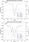 |
Fig. 1. The impact of the blending lines in the Li I λ670.8 nm region on the resulting 3D NLTE corrections. The best fitting 1D LTE spectrum (blue continuous line) is superimposed on the 3D NLTE spectrum (black dotted line) computed for Teff = 5870 K, log ℊ = 4.5, [Fe/H] = 0, A(Li)3DNLTE = 2.0, 6Li/7Li3DNLTE = 5% and representing the “observation”. The synthetic spectra are computed adopting only the Li I doublet including hyperfine structure (line list K95, upper panel), and the line list G09 (lower panel), which includes also other atomic blends. The right y-axis gives the scale of the residuals (blue dashed line). We measure A(Li) = 1.92 and 6Li/7Li = 6.1% for line list K95, and A(Li) = 1.92 and 6Li/7Li = 5.4% in case of line list G09. |
The 3D NLTE corrections (Δ∗A3DNLTE−1DLTE and Δ∗q3DNLTE−1DLTE) are computed for a grid of three A(Li)3DNLTE and three q(Li)3DNLTE values for each 3D model atmosphere given in Table 1. These corrections are meant for correcting the 1D LTE results without knowing the 3D NLTE A(Li)3DNLTE and 6Li/7Li3DNLTE of the observed spectrum, and therefore, they should not depend on the 3D NLTE values of A(Li)3DNLTE and q(Li)3DNLTE but on the measured 1D LTE values. Therefore, we converted our 3D NLTE corrections such that they depend on the 1D LTE lithium abundance, A(Li), and 1D LTE isotopic ratio, q(Li), instead of depending on the true (3D NLTE) values A(Li)3DNLTE and q(Li)3DNLTE. To do this, we used the best-fitting 1D LTE values of the lithium abundance and the 6Li/7Li isotopic ratio for each A(Li)3DNLTE and q(Li)3DNLTE point of our 3D NLTE grid and interpolated the 3D NLTE corrections to the 1D LTE values A(Li) = 1.5, 2.0, 2.5 and q(Li) = 0, 5 and 10%. All the subsequent plots and tables presented in this work will be using these 3D NLTE corrections as a function of A(Li) and q(Li), denoted as ΔA3DNLTE−1DLTE and Δq3DNLTE−1DLTE, respectively.
Figure 2 shows the 3D NLTE corrections plotted vs. Teff for 6Li/7Li (upper left panel) and A(Li) (lower left panel) for [Fe/H] = 0, A(Li) = 2.0 and q(Li) = 5%. The corrections for surface gravities 4.0 and 4.5 are plotted as blue circles and red triangles, respectively, and are connected with lines of different style for different ν sin i values. For a given log ℊ, the 3D NLTE corrections of 6Li/7Li (Δq3DNLTE−1DLTE) become larger (more negative) for higher temperatures, and they are larger for the lower log ℊ. We note that Δq3DNLTE−1DLTE depends also on ν sin i, A(Li), and q(Li): for a given log ℊ and Teff, they become smaller (more positive) for higher ν sin i, and for a given stellar parameters they will be higher for stars with higher lithium abundance and isotopic ratio. The dependence of Δq3DNLTE−1DLTE on the Vmicro used for 1D LTE spectral synthesis is negligible, and we take the central value of Vmicro as representative for this work.
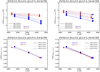 |
Fig. 2. 3D NLTE corrections Δq3DNLTE−1DLTE (upper panels) and ΔA3DNLTE−1DLTE (lower panels) vs. Teff for [Fe/H] = 0, A(Li) = 2.0, q(Li) = 5%, obtained with line lists K95 (left panels) and G09 (right panels). The blue circles and the red triangles correspond to log ℊ = 4.0 and log ℊ = 4.5, respectively. The computed 3D NLTE corrections for different υ sin i values are connected with lines of different styles (see legend). |
On the other hand, the 3D NLTE corrections for the lithium abundance, ΔA3DNLTE−1DLTE, become larger for lower effective temperatures. There is only a slight dependence on the surface gravity, and their dependence on the ν sin i can be neglected (see Fig. 2, lower left panel). The ΔA3DNLTE−1DLTE corrections do not show variations for different Vmicro and q(Li) values, whereas they are decreasing slightly with larger A(Li) values.
Similar plots for the other three metallicities of our grid are given in Appendix A. For full details, we provide electronically a table of the corrections for Teff = 5900, 6300, 6500 K, log ℊ = 4.0 and 4.5, [Fe/H] = −1.0, −0.5, 0.0, 0.5, A(Li) = 1.5, 2.0, 2.5, q(Li) = 0, 5, 10%, and ν sin i = 0.0, 2.0, 4.0, 6.0 km s−1, based on the pure lithium line list K95.
2.4.2. The impact of the mixing-length parameter
To investigate the dependence of our results on the choice of the mixing length parameter for 1D LHD models, we computed ΔA3DNLTE−1DLTE and Δq3DNLTE−1DLTE using the models N 1–6 and N 13–18 with αMLT = 0.5 and 1.5 (N 3, 15 and 17 only with αMLT = 0.5). As expected, the choice of this parameter did not affect the Δq3DNLTE−1DLTE results, while ΔA3DNLTE−1DLTE varied slightly by ±0.01 dex over the considered range of αMLT.
2.4.3. The impact of blend lines
The bottom panel of Fig. 1 shows the best fit to the 3D NLTE spectrum computed for the same parameters as in Sect. 2.4.1, but now adopting line list G09 that includes atomic and molecular blends partly overlapping with the Li feature. In this case, the 3D NLTE correction of the 6Li/7Li isotopic ratio is somewhat smaller (−0.45% points), while the 3D NLTE correction for A(Li) is similar to the K95 case (∼+0.08 dex).
Initially, we were expecting that the fitting results would depend only weakly on the adopted line list. Comparison of the lower panels of Fig. 2 shows that this is basically the case for the A(Li) correction. However, while the 6Li/7Li corrections derived with line list G09 are qualitatively similar to those obtained from fitting the pure lithium spectrum, there are quantitative differences that depend on a variety of factors.
As shown in Fig. 1 (bottom), the blends in this spectral region may be quite strong (e.g., the Fe I line at ∼670.74 nm) and can play an even greater role in the fitting procedure than the Li I line itself. We recall that the main fitting parameters are A(Li) and q(Li), both only influencing the Li line, while the two remaining fitting parameters, global Gaussian line broadening and line shift, act on the all spectral lines. However, to keep the dimensionality of the problem manageable, the strength and wavelength shift of the individual blend lines is not adjusted in the fitting procedure. This deficiency of our method can lead to meaningless fitting results, because poorly reproduced stronger blend lines determine the global line broadening and shift of the best fit, and therefore indirectly dictate an ill-defined solution for 6Li/7Li. This is especially true for the case of high metallicity ([Fe/H] = +0.5) and low lithium abundance (A(Li) = 1.5), where the 6Li/7Li corrections obtained with line list G09 are essentially useless.
It is therefore hardly surprising that line lists G09 and M12 produce somewhat different fitting results (compare Figs. 2 and A.4), which moreover depend strongly on the wavelength range selected for fitting the Li I 670.8 nm spectral region, as well as on whether the continuum placement is a free or a fixed parameter.
The above-mentioned difficulties do not exist if we derive the 3D NLTE corrections using the line list K95 which includes only the Li I components. We also notice that the results obtained with this line list are much less sensitive to the value of ν sin i than in the case of line lists G09 and M12. We argue that the fitting results obtained by considering only Li I lines must be very similar to those one would derive if all blend lines were fitted individually in the line lists G09, M12, or any other line list representative of the Li region. This argument is illustrated and supported by the investigations presented in Appendices B and C, where we show that a line list adjusted to fit a given spectrum in 1D generally produces a less satisfactory fit when used for 3D modeling. An equally good fit in 3D can only be achieved by readjusting the line list to account for 3D abundance corrections and differential wavelength shifts of the blends. When using the 1D and 3D fine-tuned line lists, respectively, the differential 1D-3D lithium isotopic abundances become largely independent of the blend lines and are well approximated by the corrections obtained with line list K95 (only Li I).
2.5. Analytical expressions
We derived analytical expressions for the corrections derived from the “only Li” line list K95 to be able to numerically evaluate ΔA3DNLTE−1DLTE and Δq3DNLTE−1DLTE as a function of the stellar parameters for any target star within the range of our grid.
As mentioned above, the A(Li) abundance corrections for all the models in our grid show only a weak dependency on the surface gravity. Assuming a log ℊ of 4.0 or 4.5, the resulting A(Li) corrections are very similar, as shown in the lower panels of Fig. 2. Within the modeling uncertainties (see below), the log ℊ dependence may be neglected. For this reason, we assumed ΔA3DNLTE−1DLTE to be independent of log ℊ while deriving the analytic approximation.
Somewhat unexpectedly, model atmosphere N2, with Teff = 5920 K, log ℊ = 4.5, [Fe/H] = −1, results in a smaller ΔA(Li) than expected from the trends of the corrections derived using other models in our grid (see Figs. A.1–A.3). A possible explanation for this discrepancy is that this model was computed for a smaller number of snapshots (8) in comparison to the other models (20). We decided not to use this result and instead consider it to be equal to the correction computed for the model N1 (with the same Teff but log ℊ = 4.0) in deriving the numerical fitting function for ΔA3DNLTE−1DLTE.
We provide a link to a web page2 that uses the analytical expressions developed in this work and allows the user to compute the Δq3DNLTE−1DLTE corrections as a function of Teff, [Fe/H], log ℊ, ν sin i, A(Li) and 6Li/7Li, and the ΔA3DNLTE−1DLTE corrections as a function of Teff, [Fe/H] and A(Li). However, below we also provide simplified analytical expressions for a quick evaluation of the 3D NLTE corrections.
The simplified expressions for ΔA3DNLTE−1DLTE and Δq3DNLTE−1DLTE provided in this section are based on all available data points for ν sin i = 2.0 km s−1, A(Li) = 2.0, q(Li) = 5%, and are functions of Teff, (log ℊ), and [Fe/H]. The two fitting functions are described by the following equations:
 (1)
(1)
 (2)
(2)
where 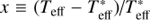 , y ≡ log ℊ − log ℊ* and z ≡ [Fe/H], with
  and log ℊ∗ = 4.0. The valid parameter ranges are 0 ≤ x ≤ 0.1; 0 ≤ y ≤ 0.5; −1.0 ≤ z ≤ +0.5. The formulae consist of six (C0−5) and 18 (cijk) numerical coefficients for ΔA and Δq, respectively (explicitly given in Table 2).
To visualize the resulting 3D NLTE corrections generated with this tool, we present in Fig. 3 the contours of ΔA3DNLTE−1DLTE in the Teff – [Fe/H] plane (upper panel), and contour plots of Δq3DNLTE−1DLTE in the Teff − [Fe/H] and Teff − log ℊ plane (middle and lower panel, respectively).
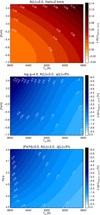 |
Fig. 3. Contour plots of 3D NLTE A(Li) corrections ΔA3DNLTE−1DLTE (upper panel) and 6Li/7Li corrections Δq3DNLTE−1DLTE (middle panel) in the Teff – [Fe/H] plane. The same 3D NLTE 6Li/7Li corrections in the Teff – log ℊ plane are shown in the bottom panel. The contours are computed for [Fe/H] = 0, ν sin i = 2km s−1, A(Li) = 2.0, and q(Li) = 5%, employing the analytical expressions in Eqs. (1) and (2) with the coefficients given in Table 2. |
The functional forms provided in this work allow a quick estimate of 3D NLTE corrections for a limited range of stellar parameters. For a complete overview and more precise 3D NLTE corrections, we refer to the table available at the CDS, and to the above-mentioned web page2. To give an example, our full analytical expressions give the following corrections for HD 82943 (Teff = 6025 K, log ℊ = 4.53, [Fe/H] = +0.30; Israelian et al. 2003): ΔA3DNLTE−1DLTE = +0.08 dex and Δq3DNLTE−1DLTE = −1.7% points.
The root mean square (rms) difference between the global fitting function used by the above-mentioned web page and the input data points of the regular grid is 0.007 dex for ΔA3DNLTE−1DLTE and 0.07% points for Δq3DNLTE−1DLTE. These numbers represent the mean fitting function errors of the two quantities for stellar parameters that lie close to our grid points.
In order to evaluate the interpolation errors of our analytical expressions outside of the grid points, we computed ΔA3DNLTE−1DLTE and Δq3DNLTE−1DLTE for intermediate Teff, log ℊ and A(Li) values by using two additional 3D model atmospheres with [Fe/H] = 0.0, log ℊ = 4.3 and Teff = 6110 and 6430 K. The 3D NLTE spectra have been computed for A(Li)3DNLTE = 1.5, 1.75, 2.0, 2.25, 2.5 and for the same 6Li/7Li and ν sin i values as in case of the original grid. The rms difference between the global fitting function and these new intermediate data points is again 0.007 dex for ΔA3DNLTE−1DLTE and 0.10% points for Δq3DNLTE−1DLTE. Even if we do not have the possibility to compute 3D NLTE corrections for intermediate points in [Fe/H], due to the lack of 3D hydrodynamical model atmospheres, we assume that the mean interpolation errors of 0.01 dex for ΔA and 0.10% points for Δq are valid for the whole parameter space covered by our grid. The largest errors in ΔA of ±0.015 dex are encountered at low temperatures (Teff ≈ 5900 K), while the largest errors in Δq of ±0.2% points are mainly incurred at high temperatures (Teff ≈ 6500 K).
2.6. 1D NLTE corrections and comparison with other works
In order to distinguish between the contributions of 3D and NLTE effects in the combined 3D NLTE correction, we repeated the same procedure for deriving the 3D NLTE corrections but replacing the grid of 3D NLTE spectra for A(Li)3DNLTE = 2.0 and q(Li)3DNLTE = 5% with an identical grid of 1D NLTE spectra. A rotational broadening of ν sin i = 2.0 km s−1 was applied to both 1D NLTE and 1D LTE spectra. The 1D NLTE corrections for 6Li/7Li are very close to zero, having a mean value of −0.10% with a standard deviation of 0.08%. This is expected as both LTE and NLTE line profiles are intrinsically symmetric. On the other hand, the 1D NLTE corrections for A(Li) show a similar trend as the 3D NLTE corrections, although with an offset to slightly smaller values (see Fig. 4). We have derived an equation similar to the Eq. (1) for the 1D NLTE case to facilitate the comparison with our 3D corrections and with the results from the literature (see below).
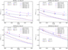 |
Fig. 4. Comparison of the 1D and 3D NLTE abundance corrections derived in this work with the 1D NLTE corrections from Lind et al. (2009; L2009, dotted lines) and Takeda & Kawanomoto (2005; T2005, dash-dotted lines) for metallicities −1.0, −0.5, 0.0, and +0.5 (from top left to bottom right). Red and blue triangles denote the individual 3D NLTE corrections, while red and blue circles denote the individual 1D NLTE corrections for A(Li) computed in this work (H2018) for log ℊ of 4.0 and 4.5, respectively. |
Figure 4 shows the functions for estimating the 3D NLTE and 1D NLTE A(Li) corrections derived in this work for metallicities [Fe/H] = −1.0, −0.5, 0.0, and +0.5, together with the results obtained by Takeda & Kawanomoto (2005) and Lind et al. (2009). Our 3D and 1D NLTE corrections follow similar trends but with small offset towards lower values (ranging between 0.01 and 0.03 dex, depending on [Fe/H] and Teff). This only small difference indicates that the 3D effects slightly enhance the non-LTE effects, while the latter generally dominate over the 3D effects in the combined 3D NLTE corrections.
The overall trends of our 1D NLTE corrections are similar to the trends obtained by Lind et al. (2009), with an offset ranging between 0.02 and 0.06 dex, depending mainly on the metallicity, while the curves of Takeda & Kawanomoto (2005) have a slightly different slope. Such differences in the 1D NLTE lithium abundance corrections, being ∼0.06 dex at most, are not unexpected due to the differences in the methods (model atmospheres, model atom, numerical procedure for computing departure coefficients, etc.) used by different authors. Nevertheless, we performed a test to check if the difference in the 1D NLTE A(Li) corrections could be explained by the different model atmospheres used in the spectral synthesis in this work (1D LHD models) and in Lind et al. (2009; MARCS models), respectively. The test was performed using a 1D NLTE spectrum computed from a MARCS model with Teff = 6500 K, [Fe/H] = −1, log ℊ = 4.0, assuming A(Li)1DNLTE = 2.0 and 6Li/7Li1DNLTE = 5 %, and a corresponding grid of 1D LTE spectra computed for combinations of nine A(Li) and nine 6Li/7Li values, using the same MARCS model atmospheres (Gustafsson et al. 2008) as in Lind et al. (2009). The MARCS NLTE spectrum was fitted by the grid of MARCS LTE line profiles following the same fitting procedure as described in Sect. 2.3. The resulting 1D LTE A(Li) correction is −0.055 dex, in very good agreement with the correction of −0.053 dex obtained for those stellar parameters by Lind et al. (2009). This result confirms that the shift of ∼0.05 dex between our 1D NLTE lithium abundance corrections and the ones by Lind et al. (2009; see Fig. 4, top left panel) are likely due to the different model atmospheres adopted in the spectral synthesis.
The analytical expressions given in Sbordone et al. (2010) for A(Li) were derived using 3D model atmospheres with metallicities −2 and −3 that do not overlap with our grid. Since we do not observe a linear dependence of the A(Li) 3D NLTE corrections on the metallicity, the extrapolated corrections from Sbordone et al. (2010) would be too uncertain for a useful comparison with our results. Therefore, we do not present such a comparison.
We compared the 3D NLTE corrections for 6Li/7Li derived in this work with the corrections presented by Steffen et al. (2012) and found very good agreement. This was expected, since the model atmospheres and methods used in these two works are similar. The present study extends the work of Steffen et al. (2012), using a 3D NLTE grid with more metallicity points around the solar value, and also investigating the dependence of the 3D NLTE corrections on A(Li), 6Li/7Li, ν sin i, and the list of blend lines.
3. Li abundance and 6Li/7Li isotopic ratio in HD 207129 and HD 95456
In this section, we analyze two solar-type stars, HD 207129 and HD 95456, in order to determine A(Li) and the 6Li/7Li isotopic ratios, at first with a 1D LTE approach, and afterwards applying our already pre-computed 3D NLTE corrections. These stars have been selected for this study because the difference in their effective temperatures places them at two extreme positions in our correction grid. They are part of a larger sample of stars with high lithium content and low activity levels, for which high-resolution and very-high-S/N spectra are available that allow a sensitive analysis of 6Li/7Li. We point out that Gomes da Silva et al. (2014) performed long-term activity studies of HD 207129 and HD 95456 using Ca II H & K and Hα lines in their HARPS spectra (Mayor et al. 2003), and found both stars to show very low activity levels with no significant long-term variability.
3.1. Observations and stellar parameters
The observed spectra used in this work have been obtained with the HARPS spectrograph at La Silla observatory (ESO, Chile) within the framework of the HARPS GTO planet search program (subsample HARPS-I, Mayor et al. 2003). The spectral resolution of R ∼ 115 000 and the high S/N of ∼2000 of the combined spectrum of each star provide the quality that is needed for analysis of the Li I λ670.8 nm region in the context of the 6Li/7Li measurements.
The stellar atmospheric parameters (Teff, log ℊ, [Fe/H] and Vmicro) of both stars were derived by Sousa et al. (2008) and are summarized in Table 3. The abundances of several elements with blending lines present in the line lists (Si, Ca, Ti, V) were adopted from Adibekyan et al. (2012), whereas the carbon and oxygen abundances were taken from Suárez-Andrés et al. (2017) and Bertran de Lis et al. (2015), respectively, and the nitrogen abundance was chosen to be equal to the carbon abundance. The elemental abundances adopted for the Sun, HD 207129, and HD 95456 are given in Table 4.
Chemical abundances A(X) used in this work.
3.2. Rotational broadening and iron abundance
A list of atomic line data has been constructed for a number of isolated, unblended Fe I lines taken from Doyle et al. (2014), Tsantaki et al. (2013) and from the VALD-v3 database (Kupka et al. 2011) to estimate the projected rotational velocity (ν sin i) and the possible small iron abundance correction for the stars studied in this work. For each line of each star, a grid of nine 1D LTE Kurucz Atlas spectra was computed assuming an iron abundance range of ±0.2 dex around the adopted iron abundance (metallicity) value, with a step of 0.05 dex. The spectra were computed using the 2014 version of the spectral synthesis code MOOG (Sneden 1973).
The fitting procedure was performed for the solar flux atlas from Kurucz (2005), and for the HARPS spectra of HD 207129 and HD 95456. The HARPS spectra have been locally normalized for each Fe line. We investigated the quality of the fits by eye and by means of a  analysis. All the lines that seemed to be blended with other spectral features (at least in one of the two stars or the Sun), or which provided a non-satisfactory fit to the observations, were excluded from the sample. Eventually, we were left with 10 “clean” Fe I lines which are well isolated and can be fitted well in the solar spectrum and the HARPS spectra of the two stars. Table 5 lists the atomic data of the selected Fe I lines: wavelength, excitation potential (EP), oscillator strength (log ℊ f), and the reference to the source they were taken from for each individual Fe I line.
Four parameters were varied to achieve the best fit: [Fe/H], ν sin i, the global wavelength shift (Δυ), and the continuum level. Since it was difficult to obtain both Vmacro and ν sin i individually from the fitting procedure due to a “degeneracy” of the solution, a fixed Gaussian macroturbulence velocity (Vmacro) was assumed for the fitting. Vmacro was adopted from Doyle et al. (2014) and used after the application of a factor to convert the radial-tangential (RT) macroturbulence parameter (VRT) provided by these authors to the Gaussian macroturbulence parameter Vmacro that we use. This conversion factor was determined for the solar case using the same solar ν sin i and atmospheric parameters (including Vmicro = 1.0 km s−1) as assumed in Doyle et al. (2014). We derive a solar [Fe/H] = −0.02 ± 0.06 and Vmacro = 2.12 ± 0.10 km s−1 resulting in the conversion formula Vmacro ∼ 0.66 VRT. The relation between the different macroturbulence velocity models has been discussed in a recent work by Takeda & UeNo (2017), and the conversion factor of 0.66 that we derive is in agreement with their results. For a given Vmacro, each line profile has been broadened by nine different ν sin i values with the flux convolution approximation, assuming a limb darkening coefficient of ε = 0.6 (Gray 2005). The least-squares fitting method that we apply (MPFIT; Markwardt 2009) relies on interpolation in the grid of the precomputed synthetic spectra with different [Fe/H] and ν sin i. For each star, the best fit values of [Fe/H] and ν sin i were averaged over the ten different Fe I lines and the uncertainties were derived from the standard deviations (cf. Table 5).
For HD 207129, we obtain ν sin i = 2.21 ± 0.24 km s−1 and an iron abundance correction of Δ[Fe/H] = −0.025 ± 0.063 dex. For HD 95456, the radial-tangential macroturbulence is VRT = 5.05 km s−1 according to Doyle et al. (2014), which is large enough to broaden the synthetic line profiles to such an extent that the fits were not very different for ν sin i between 0 and 3 km s−1. For instance, when we use the Vmacro value from Doyle et al. (2014), we obtain a formal ν sin i of 0.88 km s−1. As we discuss in Sect. 3.5, the measured A(Li) and 6Li/7Li for HD 95456 essentially do not change with different ν sin i assumptions. We therefore prefer the ν sin i value of 3.28 km s−1 determined by Delgado Mena et al. (2015), based on a combination of Fourier transform and goodness-of-fit methods. We derive a small Fe abundance correction of Δ[Fe/H] = −0.068 ± 0.067 dex (relative to the literature value of [Fe/H]) for HD 95456.
Fe I lines used for deriving ν sin i and the iron abundance correction Δ[Fe/H].
3.3. Blend lines in the lithium λ670.8 nm region
One of the challenges in 6Li/7Li measurements is the presence of several other atomic and molecular lines overlapping with the resonance doublet. While the contribution of these blends may be very small in metal poor stars, they become more significant at higher metallicities and must be treated carefully for stars having metallicities close to solar or higher. There are several lists of atomic and molecular lines currently available in the literature which have been carefully constructed to reproduce the Li λ670.8 nm region (e.g., Mandell et al. 2004, Ghezzi et al. 2009, Meléndez et al. 2012, Israelian 2014; priv. comm.) and are fitted for very sensitive measurements of the 6Li/7Li isotopic ratio in solar-type stars. It has already been demonstrated that the use of different lists of atomic and molecular lines interfering with the Li I λ670.8 nm doublet can lead to noticeable differences in the measured values of 6Li/7Li (e.g., Israelian et al. 2003; Mott et al. 2017). We therefore perform our analysis using different line lists provided in the literature and compare the results.
Specifically, we used three different line lists for the analysis of A(Li) and 6Li/7Li in the atmospheres of HD 207129 and HD 95456. In addition to G09 and M12, we used the line lists constructed by Israelian (2014; priv. comm.), as given by Mott et al. (2017; hereafter, I14). The line lists were adjusted by computing 1D LTE synthetic spectra and fitting the 670.8 nm region in the solar spectrum (G09) or in spectra of other stars (I14). The above authors assumed different elemental abundances from what we assume for the Sun (Table 4, Col. 2). Specifically, we adopted the solar abundance values for 12 elements (Li, C, N, O, P, S, K, Fe, Eu, Hf, Os, Th) from Caffau et al. (2011; their Table 5), and for other elements we used the internal solar elemental abundances of the 2014 version of MOOG, which is based on the solar abundances recommended by Asplund et al. (2009).
A molecule that is present in all line lists representing the Li I 670.8 nm region is CN. The presence of several lines of this molecule is important in the 6Li determination, and assuming the correct C, N, and O abundances (because O can influence the equilibrium of the molecular reaction network) can be crucial. Particularly, the assumptions for solar abundances of O and N were significantly different between the authors of the line lists and our work. Therefore, we made some calibrations to eliminate the differences arising from different assumptions of solar abundances while constructing the line lists for performing our 6Li/7Li analysis. In case of O and N, our abundances were lower by up to 0.17 and 0.19 dex, respectively, and by 0.06 dex for C. In this case, we have scaled the log ℊ f values of all the CN lines in this region by a constant factor. This factor was derived by fitting the solar flux atlas with a pre-computed grid of 1D LTE synthetic spectra for the Sun. For each line list, a grid of 1D LTE spectra was computed applying different factors (within the range of ±0.3 dex with a step of 0.01 dex) to the log ℊ f values of all the CN lines. Then, for a given line list, we adopted the log ℊ f factor resulting in the best fit (χ2 minimization) to the solar flux atlas. This factor was +0.20 dex in case of the G09 and M12 line lists, and +0.19 dex in case of the I14 line list. For elements other than C, N, and O present in the line lists, the small solar abundance differences were taken into account by applying corresponding corrections to the log ℊ f values of the individual lines of each element. After this adjustment, all line lists are “normalized” to our adopted solar abundances.
In addition, the wavelength and the log ℊ f value of the V I line at 670.81096 nm have been updated according to the recently published values by Lawler et al. (2014). This blend is positioned close to one of the 6Li components and may affect the result of the 6Li/7Li determination if incorrect line parameters are assumed (see Sect. 3.7).
3.4. Spectral synthesis for A(Li) and 6Li/7Li studies of HD 207129 and HD 95456
In order to derive A(Li) and 6Li/7Li in the two solar-type stars, we perform a standard 1D LTE analysis using the 2014 version of the spectral synthesis code MOOG (Sneden 1973) together with Kurucz ATLAS9 1D model atmospheres (Kurucz 1993).
A grid of 1D LTE synthetic spectra has been computed for each star. The precomputed line profiles cover a range in lithium abundance defined by the expected A(Li) (literature value, Delgado Mena et al. 2015) ±0.5 dex with a step of 0.05 dex, and a range in q(Li) between 0 and 20% with a step of 1%.
For each star, the third dimension of the grid is defined by a variation of the C, N, O abundances. These abundances were scaled together by the same factor within a range of ±0.2dex around the fiducial C, N, O abundances and with a step of 0.05 dex, such that the grid of spectra includes nine different CNO values. The Fe I line at ∼670.74 nm, being one of the strongest blends in this region, can also play an important role in the 6Li/7Li analysis. Therefore, we extend our grid by computing the spectra with different [Fe/H] values, which vary around the fiducial Fe abundance by ±0.1 dex, with a step of 0.1 dex for HD 207129 and 0.05 dex for HD 95456.
Thus, a four-dimensional (4D) grid of 1D LTE spectra is obtained for combinations of 21 A(Li), 21 6Li/7Li, nine CNO abundances, and three (five) different [Fe/H] values, both for HD 207129 and HD 95456. In addition, these grids of spectra for both stars were replicated for three different line lists (G09, M12, I14). For the estimation of the systematic errors of A(Li) and 6Li/7Li due to uncertainties in effective temperature and surface gravity, the 4D grids for both stars were also computed for model atmospheres with Teff ± 50 [K] and log ℊ ± 0.1, but only for line list G09, and for the Fe and CNO abundance correction factors from the best fit for that line list. In total, 37485 and 61299 1D LTE synthetic spectra were computed for HD 207129 and HD 95456, respectively.
3.5. Fitting procedure for the HARPS spectra
To fit the observed spectra of the two target stars, we followed a procedure similar to the one already described in Sect. 2.3. The HARPS spectra of HD 207129 and HD 95456 were fitted through interpolation across a grid of 1D LTE line profiles computed with MOOG for line lists G09, M12 and I14. To achieve the best fit evaluated by means of a  minimization method, four free parameters were varied: A(Li), q(Li), the global wavelength shift (Δυ) and the FWHM of the Gaussian line broadening, which accounts also for Vmacro, while ν sin i and Vmicro are fixed at the values given in Table 3. Additionally, for each combination of stellar parameters and line list, we used the 1D LTE spectra assuming different Fe, and CNO abundances. This allowed us to achieve an even better fit, allowing for possible small abundance deviations from the adopted values. We applied a similar fitting procedure to derive the lithium abundance and 6Li/7Li isotopic ratio in the Sun (Sect. 3.8).
3.6. Fitting results for HD 207129 and HD 95456
Figure 5 shows the best 1D LTE fit to the HD 207129 (left panels) and HD 95456 (right panels) HARPS spectra, obtained with line lists G09, M12, and I14 (from top to bottom). The best fit with line list G09 is achieved for Δ [Fe/H] = −0.025 and Δ CNO = −0.05 for HD 207129, resulting in A(Li) of 2.30 and 6Li/7Li of 0.2% in this star. For HD 95456, the best fit with line list G09 is obtained for Δ [Fe/H] = −0.018 and for Δ CNO = −0.05, resulting in A(Li) = 2.65 and 6Li/7Li = 2.8%. The Gaussian Vmacro for which the best fit is achieved is 2.29 and 2.61 km s−1 for HD 207129 and HD 95456, respectively. For HD 207129, this Vmacro is in good agreement with the Vmacro used for fitting the Fe I lines given in Table 5 (Sect. 3.2). For HD 95456, the Vmacro derived with this procedure is lower, since we adopted a larger ν sin i (Table 3) than its resulting value from the fitting of the Fe I lines (Sect. 3.2). The errors given in Fig. 5 are the 1 σ formal fitting errors. The 1D LTE best-fit values for A(Li) and 6Li/7Li for all three line lists are collected in Table 6. The different line lists result in somewhat different 6Li/7Li for the same star. We adopt the results obtained using line list G09 as the representative result of our analysis since 6Li/7Li obtained with this set of blends falls between the values from the analysis with line lists M12 and I14. The uncertainty due to the different line lists is included as one contribution to the total error (see below).
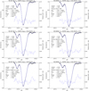 |
Fig. 5. The best fitting 1D LTE spectrum (solid line) superimposed on the HARPS spectrum (dots) for HD 207129 (left panels) and HD 95456 (right panels). The synthetic line profiles are computed adopting the line lists G09, M12, and I14 (from top to bottom), with modifications described in Sect. 3.3. The right y-axis defines the scale of the residuals (dashed line). |
Figure 6 shows the best fitting  values obtained by fitting the HARPS spectra of HD 207129 (upper panel) and HD 95456 (lower panel) with synthetic 1D LTE spectra computed for all the combinations of Fe and CNO abundances based on the preferred line list G09. From this figure, it is clear that the lowest
  values are obtained around the adopted abundances of Fe and CNO. We note that the best fits shown in Fig. 5 are based on the optimal choice of [Fe/H] and CNO derived from Fig. 6.
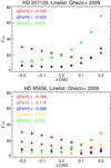 |
Fig. 6. The best |


The 3D NLTE corrections for the lithium abundance and 6Li/7Li for HD 207129 and HD 95456 were obtained using the analytical approximations developed in this work. The 3D NLTE corrections of A(Li) were computed as a function of Teff, [Fe/H], and A(Li), the 3D NLTE corrections of 6Li/7Li as a function of Teff, log ℊ, [Fe/H], ν sin i, A(Li) and 6Li/7Li. We derive 3D NLTE A(Li) corrections of +0.07 dex and +0.05 dex, and 6Li/7Li corrections of −1.1 and −1.9% points for HD 207129 and HD 95456, respectively. Afterwards, we applied these corrections to the measured 1D LTE best-fitting values of A(Li) and 6Li/7Li. The derived values after such corrections are also presented in Table 6.
We compute the errors of the 1D LTE lithium abundance and 6Li/7Li by considering seven sources of uncertainty: uncertainties related to the choice of the effective temperature (ΔTeff = ±50 [K]) and surface gravity (Δlog ℊ = ±0.1) as well as the continuum placement (1.0 ± 0.05%), the internal fitting error, the fitting errors related to different Fe (Δ [Fe/H] is ±0.1 for HD 207129 and ±0.05 for HD 95456) and CNO abundance factors (Δ CNO = ±0.05). These six errors are computed for the line list G09. The seventh error is related to the different lists of atomic and molecular blends used in this work, and for both lithium abundance and isotopic ratio is computed as the standard deviation of measured A(Li) and 6Li/7Li, respectively, adopting line lists G09, M12, and I14. These seven different error contributions are combined in quadrature and are given as the total error in Table 6.
Finally, to test the dependence of our results on the used ν sin i value, we applied a ν sin i of 0.85 km s−1 to the synthetic spectra of HD 95456, as measured in Sect. 3.2 using Fe I lines, and repeated the fitting procedure for the best fitting values of Fe and CNO abundance for the line list G09. The resulting LTE values of A(Li) = 2.65 and q(Li) = 2.7% are in very good agreement with the values derived assuming ν sin i = 3.28 km s−1, demonstrating that an accurate determination of the rotational broadening is not critical.
3.7. Tests with the SiI and VI lines
As mentioned in Sect. 3.3, the measurement of the 6Li/7Li isotopic ratio is sensitive to the list of atomic and molecular lines adopted for the spectral synthesis. In the case of HD 95456, we find a difference as high as ∼2.2%, where the lowest 6Li/7Li is 0.8% when the M12 line list is adopted, and the highest 6Li/7Li is 3.0% when I14 is used (see Table 6). The differences among the line lists arise not only from the adopted atomic data of specific lines (wavelength, log ℊ f, excitation potential), but also from the different chemical elements present in each particular list of blends.
The Si I 670.8025 nm line is of particular interest since it lies very close to the 6Li feature and has been shown to have an impact on the 6Li/7Li measurements (e.g., Israelian et al. 2001, 2003). This line was first introduced by Müller et al. (1975) in their analysis of the solar spectrum and later investigated in detail by Israelian et al. (2003) in a number of solar-type metal-rich stars. The latter authors have shown that the Si I line at 670.8025 nm is the best candidate for this unidentified feature severely blended with the 6Li line. We also note that this line has been assigned different parameters in the three line lists we use in this work. While the wavelength differences are rather small (670.8023 nm in G09 and M12, and 670.8025 nm in I14), the log ℊ f values are quite different (−2.91 in G09, −2.80 in M12 and −2.97 in I14).
In a recent work by Bensby & Lind (2018), the authors noted that new laboratory measurements showed no sign of a Si I line at 670.8025 nm, referring to a private communication source (Henrik Hartmann). However, as it has been demonstrated that a “fictitious” Si I line with the assigned atomic parameters is able to reproduce the unknown blend rather well (Müller et al. 1975; Israelian et al. 2003; Mandell et al. 2004), it is still the best choice for a reliable 6Li/7Li analysis in solar-type stars. By no means should the new measurements be taken as justification to simply remove the “fictitious” Si I line from the list of blends, as long as the unknown feature has not been unambiguously identified.
We tested to what extent the differences in the Si I line parameters, particularly in the log ℊ f value, can affect the 6Li/7Li measurement. For this purpose, we performed the same 1D LTE analysis as described in Sect. 3.5, but for different silicon abundance values at fixed Fe and CNO abundance. For each silicon abundance, the grid of lithium abundances covers 21 A(Li) times 21 6Li/7Li values. This test is performed for HD 95456 only, where the derived 1D LTE 6Li/7Li appears to be significantly different from zero.
Figure 7 shows the  (upper panel) of the best fit and the resulting 6Li/7Li (middle panel) plotted vs. the deviation (in dex) from the adopted silicon abundance for line lists G09 (red circles), M12 (green triangles), and I14 (blue stars). It is worth noting that, when the silicon abundance is reduced, the measured 6Li/7Li increases, showing that changing the silicon abundance by just 0.1 dex can alter the measured 6Li/7Li by more than 1% point for this star, while the reduced
  value changes only marginally. Furthermore, after increasing the Si abundance by a certain amount, depending on the line list (+0.3, +0.2, and +0.4 dex for G09, M12 and I14, respectively), the measured 6Li/7Li reaches 0%, indicating that the potential 6Li feature is fully (over-)compensated by the Si I line.
 |
Fig. 7. The best-fitting |


This test shows that the atomic data of this particular blend line are very important for the measurements of 6Li/7Li in solar-type stars, as suggested by Israelian et al. (2003), and might be the main factor responsible for the differences in the results achieved with the different line lists. It is worth noting that the log ℊ f of this line was calibrated by Israelian et al. (2003) in high-S/N spectra of several solar-type stars (as well as the Sun) with different effective temperatures and metallicities. In the alternative case of G09 and M12 line lists, the log ℊ f of this line and of other blend features have been adjusted in order to better reproduce the solar spectrum.
In fact, if we assume the same log ℊ f for the Si I line in all the line lists, the results appear to be in very good agreement despite differences in the other adopted blends. This shows that differences in log ℊ f of the Si I line are indeed the reason for the differences in the 6Li/7Li isotopic ratio. We can assume that this is generally the case, at least for stars with atmospheric parameters similar to HD 95456.
Because of the recently revised log ℊ f of the V I blend, we repeat the same test as above also for the V I line. Lawler et al. (2014) gave a log ℊ f higher by 0.3–0.5 dex, dependent on the line list considered. The resulting plot (Fig. 7, lower panel) indicates that this line does not considerably affect the 6Li/7Li measurement, giving differences of Δq ∼ 1% point for a 1-dex change in the vanadium abundance. Therefore, this line is not expected to change the 6Li/7Li result significantly, at least for stars with stellar parameters similar to HD 95456.
3.8. Fitting results for the Sun
We applied a similar fitting procedure to derive the lithium abundance and the 6Li/7Li isotopic ratio in the Sun by fitting the solar flux atlas of Kurucz (2005). The 1D LTE synthetic line profiles were computed from a solar ATLAS9 model (Teff = 5770 K, log ℊ = 4.44, Vmicro = 1.24 km s−1, αMLT = 1.25; see Kurucz 1993) with MOOG for combinations of 21 A(Li) and 21 6Li/7Li values, assuming a rotational broadening of ν sin i = 1.9 km s−1.
Using line list G09 (with modifications described in Sect. 3.3) and fixing the continuum level at c1 = 0.9975 (relative to the continuum placement of the solar flux atlas) as in Ghezzi et al. (2009), the best fit was obtained for A(Li) = 0.99 ± 0.01 dex and 6Li/7Li = 0.12 ± 2.0% (Case A, Table 6), where the errors are the 1 σ formal fitting errors. The derived isotopic ratio close to zero reflects the fact that Ghezzi et al. (2009) constructed their line list under the assumption that 6Li/7Li = 0. An even better fit of the solar Li region can be achieved by allowing small adjustments in the continuum level and in the abundances of Fe and CNO, as described above for the stellar fits. In this case, the best fit was obtained for c1 = 0.9977, A(Li) = 0.98 ± 0.015 dex and 6Li/7Li = 1.71 ± 2.9% (Case B, Table. 6). Allowing in addition slight adjustments of the Si and V abundances leads to a marginal improvement of the fit, but with even larger formal fitting errors: c1 = 0.9977, A(Li) = 0.98± 0.02 dex, 6Li/7Li = 0.71 ± 4.1% (Case C, Fig. 8).
For the Sun, our grid of 3D NLTE corrections suggests (after slight extrapolation) ΔA3DNLTE−1DLTE ∼ +0.1 dex and Δq3DNLTE−1DLTE ∼−0.73%, while the direct calculation of the corrections from 3D NLTE and 1D LHD synthetic solar Li line profiles by the method described in Sect. 2.3 yields ΔA3DNLTE−1DLTE ∼ +0.1 dex and Δq3DNLTE−1DLTE ∼−0.83%.
After applying the 3D NLTE correction for A(Li) to our 1D LTE best fit result (Case C), we obtain A(Li) = 1.08±0.03, where the error is estimated from measurements with different continuum locations (best fit location ±0.05%). The 6Li/7Li isotopic ratio obtained from the best 1D LTE fit (Fig. 8) is −0.1% after application of the 3D NLTE correction of −0.83%, with a large formal fitting error of ±4%.
 |
Fig. 8. The best fitting 1D LTE ATLAS/MOOG spectrum (dashed line) superimposed on the solar flux atlas spectrum of Kurucz (2005; black dots), fixing the continuum level at 0.9977 (relative to the continuum placement of the flux atlas), and using line list G09 (with modifications described in Sect. 3.3) and slight adjustments in the strengths of the CN, Fe, Si, and V lines (see Case C, Table 6) The right y-axis defines the scale of the residuals (thin blue line). |
The lithium abundance obtained in this way is in very good agreement with a recent 3D NLTE analysis of a very-high-resolution PEPSI spectrum of the Li I λ 670.8 nm region of the Sun by Strassmeier et al. (2018) who measured A(Li) = 1.09 ± 0.04. Their estimate of 6Li/7Li = 1.4 ± 1.6% agrees with our above 6Li/7Li value within the large error bars.
We point out that Strassmeier et al. (2018) also employed line list G09, which is custom-made for 1D modeling and therefore leads to an inferior fit when used unaltered for 3D spectrum synthesis. This is very likely the reason why the derived 6Li/7Li is not fully consistent with our corrected 1D result, 6Li/7Li ≈ 0. A more consistent fit in 3D can only be achieved if the line list is adapted to account for 3D effects, in particular adjusting the strength and wavelength of the silicon line (see Appendix B). We present a detailed comparison of fine-tuned 3D and 1D fits to the solar Li I λ 670.8 nm spectral region in Appendix C.
4. Summary and conclusions
We presented 3D NLTE corrections for lithium abundance, A(Li), and the 6Li/7Li isotopic ratio, q(Li), based on a six-dimensional grid of 3D NLTE spectra. The stellar parameters defining the grid are effective temperatures, Teff (3 different values), gravity, log ℊ (2), microturbulence velocity, Vmicro (3), metallicity, [Fe/H] (4), lithium abundance, A(Li)3DNLTE (3), and isotopic ratio, q(Li)3DNLTE (3; see Sect. 2 for details). In addition, four different ν sin i values of rotational broadening were applied to the 3D NLTE and 1D LTE spectra. For each list of atomic and molecular blend lines (K95, G09, and M12), this results in a total of 2592 3D NLTE corrections for both A(Li) and q(Li). The results obtained using the line lists G09 and M12 depend strongly on the wavelength range selected for fitting the Li I 670.8 nm spectral region, as well as on whether the continuum placement is a free or a fixed parameter. As a consequence, the 3D NLTE 6Li/7Li corrections depend on the atomic and molecular blends used for the spectral line synthesis. Eventually, we rely only on the 3D NLTE corrections based on line list K95 (Li only). This definition is supported by detailed fits of the solar Li spectral region with both 1D- and 3D-based synthetic spectra computed with fine-tuned line lists (Appendix C).
6Li/7Li derived by fitting a given 3D NLTE spectrum with the grid of 1D LTE line profiles is found to be always larger than the input 3D NLTE values by 0.4–4.9% for the range of stellar parameters studied in this work. This implies that a 1D LTE spectral analysis leads to an overestimation of the 6Li/7Li isotopic ratio by up to 4.9% points in solar-type stars covered by our grid. The 3D NLTE corrections, Δq3DNLTE−1DLTE, are therefore always negative.
The corrections show a systematic dependence on the stellar parameters. For a given metallicity, generally Δq3DNLTE−1DLTE becomes larger with higher Teff and lower log ℊ. For given Teff and log ℊ, they become larger with higher metallicity, A(Li), and isotopic ratio q(Li). Moreover, we observe a dependence of Δq3DNLTE−1DLTE on the applied rotational broadening: the higher the ν sin i, the smaller the corrections. Furthermore, the quality of the fit improves assuming higher ν sin i values applied simultaneously to the 3D NLTE and 1D LTE spectra, leading to lower values of  (but also implying larger fitting errors). On the other hand, we observe only a very weak variation of Δq3DNLTE−1DLTE with the small changes (±0.5 km s−1) of the microturbulence parameter, and therefore adopt the results obtained assuming the central Vmicro values as representative corrections.
Similarly, the abundance corrections, ΔA3DNLTE−1DLTE, show a systematic dependence on the stellar parameters. For a given [Fe/H], they generally become larger towards lower Teff. We observe small variations of ΔA3DNLTE−1DLTE for different log ℊ values (4.0 or 4.5) and A(Li), whereas the dependence on 6Li/7Li, Vmicro, and ν sin i is negligible. The 3D NLTE correction for A(Li) turned out to be very similar for different lists of the atomic and molecular data used for the spectral line synthesis. They are found to range between −0.01 and +0.11 dex.
We provide analytical expressions (Eqs. (1) and (2)) which allow to estimate the 3D NLTE correction for A(Li) and 6Li/7Li as a function of Teff, log ℊ, and [Fe/H] (see Sect. 2.5). These mathematical functions are valid for the representative values A(Li) = 2.0, q(Li) = 5%, and ν sin i = 2km s−1 for a quick evaluation of the 3D NLTE corrections in the investigated range of stellar parameters. For full details, we provide a (electronic) table with the complete grid of the 3D NLTE corrections, and a link to a web page that allows the user to compute the 3D NLTE corrections of A(Li) as a function of Teff [Fe/H], and A(Li), and the 3D NLTE corrections of 6Li/7Li as a function of Teff, log ℊ, [Fe/H], ν sin i, A(Li) and 6Li/7Li.
Our analytical expressions, valid for solar-type stars, allow to account for 3D plus NLTE effects without the need of direct access to complex 3D NLTE computations. This is particularly important when a large sample of stars needs to be analyzed in terms of lithium abundance and isotopic ratio, since 3D NLTE analysis for even a single target is computationally demanding and time consuming. The analysis of the observed spectra can be carried out at first by using standard 1D LTE spectrum synthesis techniques. Afterwards, the 1D results can be corrected for the 3D NLTE effects by applying the precomputed 3D NLTE corrections interpolated to the desired set of stellar parameters.
In the second part of this work, we use high-quality HARPS spectra of two solar-type stars in order to derive the A(Li) and 6Li/7Li in their atmospheres. The stars were selected because they are located at opposite sides of the investigated Teff range where the corrections show the largest differences. The lithium doublet in these two stars was first analyzed with a standard 1D LTE approach, and subsequently corrected for 3D NLTE effects using the pre-computed 3D NLTE corrections. After applying the 3D NLTE corrections, we obtain A(Li) = 2.37 ± 0.04 and 6Li/7Li = −0.9% ± 0.7% for HD 207129, whereas we derive A(Li) = 2.70 ± 0.04 and 6Li/7Li = 0.9%±1.4% for HD 95456. The correction for 6Li/7Li is estimated to be Δq3DNLTE−1DLTE = −1.1% for HD 207129 and Δq3DNLTE−1DLTE = −1.9% for HD 95456.
In the case of HD 95456, the 2σ detection of 6Li in the 1D LTE analysis is turned into a clear non-detection after applying the 3D NLTE correction. In conclusion, we do not find significant amounts of 6Li in either of the two stars.
Additionally, we studied the impact of two weak absorption lines (Si I, V I) on our 6Li/7Li measurements in HD 95456, and concluded that the Si I 670.8025 nm feature is the most critical blend for this analysis, confirming the result of Israelian et al. (2003).
Finally, we have demonstrated that a list of blend lines that are adjusted (like G09) by fine-tuning log ℊ f-values and wavelength positions to yield a perfect fit to the solar Li spectral region with a particular 1D model atmosphere cannot be expected to produce an equally good fit when employed unaltered for 3D modeling. For this reason, fitting 3D model spectra directly to observations may not always be the most desirable approach.
A(X) = log(N(X)/N(H)) + 12, where X is the chemical element.
The asymmetric 3D profile of the Fe line at λ 670.74 nm is represented by two components in 1D.
Acknowledgments
This work has made use of the VALD database, operated at Uppsala University, the Institute of Astronomy RAS in Moscow, and the University of Vienna. We thank the Leibniz-Association for supporting G.H. and A.M. through a SAW graduate school grant. JIGH acknowledges financial support from the Spanish ministry project MINECO AYA2014-56359-P and from the Spanish Ministry of Economy and Competitiveness (MINECO) under the 2013 Ramón y Cajal program MINECO RYC-2013-14875. We thank János Bartus for creating the web page calculator. Finally, we thank the anonymous referee for his/her critical questions which helped us to improve the presentation of our results.
References
- Adibekyan, V. Z., Sousa, S. G., Santos, N. C., et al. 2012, A&A, 545, A32 [NASA ADS] [CrossRef] [EDP Sciences] [Google Scholar]
- Asplund, M., Grevesse, N., Sauval, A. J., & Scott, P. 2009, ARA&A, 47, 481 [NASA ADS] [CrossRef] [Google Scholar]
- Bensby, T., & Lind, K. 2018, A&A, 615, A151 [NASA ADS] [CrossRef] [EDP Sciences] [Google Scholar]
- Bertran de Lis, S., Delgado Mena, E., Adibekyan, V. Z., Santos, N. C., & Sousa, S. G. 2015, A&A, 576, A89 [NASA ADS] [CrossRef] [EDP Sciences] [Google Scholar]
- Caffau, E., Ludwig, H.-G., Steffen, M., et al. 2008, A&A, 488, 1031 [CrossRef] [EDP Sciences] [Google Scholar]
- Caffau, E., Ludwig, H.-G., Steffen, M., Freytag, B., & Bonifacio, P. 2011, Sol. Phys., 268, 255 [NASA ADS] [CrossRef] [Google Scholar]
- Carlsson, M., Rutten, R. J., Bruls, J. H. M. J., & Shchukina, N. G. 1994, A&A, 288, 860 [NASA ADS] [Google Scholar]
- Cayrel, R., Steffen, M., Chand, H., et al. 2007, A&A, 473, L37 [NASA ADS] [CrossRef] [EDP Sciences] [Google Scholar]
- Cuntz, M., Saar, S. H., & Musielak, Z. E. 2000, ApJ, 533, L151 [NASA ADS] [CrossRef] [PubMed] [Google Scholar]
- Delgado Mena, E., Bertrán de Lis, S., Adibekyan, V. Z., et al. 2015, A&A, 576, A69 [NASA ADS] [CrossRef] [EDP Sciences] [Google Scholar]
- Doyle, A. P., Davies, G. R., Smalley, B., Chaplin, W. J., & Elsworth, Y. 2014, MNRAS, 444, 3592 [NASA ADS] [CrossRef] [Google Scholar]
- Dutra-Ferreira, L., Pasquini, L., Smiljanic, R., Porto de Mello, G. F., & Steffen, M. 2016, A&A, 585, A75 [NASA ADS] [CrossRef] [EDP Sciences] [Google Scholar]
- Forestini, M. 1994, A&A, 285, 473 [Google Scholar]
- Freytag, B., Steffen, M., & Dorch, B. 2002, Astron. Nachr., 323, 213 [NASA ADS] [CrossRef] [EDP Sciences] [Google Scholar]
- Freytag, B., Steffen, M., Ludwig, H.-G., et al. 2012, J. Comput. Phys., 231, 919 [Google Scholar]
- Ghezzi, L., Cunha, K., Smith, V. V., et al. 2009, ApJ, 698, 451 [G09] [NASA ADS] [CrossRef] [Google Scholar]
- Gomes da Silva, J., Santos, N. C., Boisse, I., Dumusque, X., & Lovis, C. 2014, A&A, 566, A66 [NASA ADS] [CrossRef] [EDP Sciences] [Google Scholar]
- Gray, D. F. 2005, The Observation and Analysis of Stellar Photospheres, 3rd edn. (Cambridge, UK: Cambridge Univ. Press) [CrossRef] [Google Scholar]
- Gustafsson, B., Edvardsson, B., Eriksson, K., et al. 2008, A&A, 486, 951 [NASA ADS] [CrossRef] [EDP Sciences] [Google Scholar]
- Howk, J. C., Lehner, N., Fields, B. D., & Mathews, G. J. 2012, Nature, 489, 121 [NASA ADS] [CrossRef] [PubMed] [Google Scholar]
- Israelian, G., Santos, N. C., Mayor, M., & Rebolo, R. 2001, Nature, 411, 163 [NASA ADS] [CrossRef] [PubMed] [Google Scholar]
- Israelian, G., Santos, N. C., Mayor, M., & Rebolo, R. 2003, A&A, 405, 753 [NASA ADS] [CrossRef] [EDP Sciences] [Google Scholar]
- Kawanomoto, S., Kajino, T., Aoki, W., et al. 2009, ApJ, 701, 1506 [NASA ADS] [CrossRef] [Google Scholar]
- Klevas, J., Kučinskas, A., Steffen, M., Caffau, E., & Ludwig, H.-G. 2016, A&A, 586, A156 [NASA ADS] [CrossRef] [EDP Sciences] [Google Scholar]
- Kupka, F., Dubernet, M. L., & VAMDC Collaboration. 2011, Bal. Astron., 20, 503 [Google Scholar]
- Kurucz, R. 1993, ATLAS9 Stellar Atmosphere Programs and 2 km/s grid. Kurucz CD-ROM No. 13 (Cambridge, MA: Smithsonian Astrophysical Observatory), 13 [Google Scholar]
- Kurucz, R. L. 1995, ApJ, 452, 102 [NASA ADS] [CrossRef] [EDP Sciences] [Google Scholar]
- Kurucz, R. L. 2005, Mem. Soc. Astron. It. Sup., 8, 189 [NASA ADS] [Google Scholar]
- Lawler, J. E., Wood, M. P., Den Hartog, E. A., et al. 2014, ApJS, 215, 20 [NASA ADS] [CrossRef] [Google Scholar]
- Lind, K., Asplund, M., & Barklem, P. S. 2009, A&A, 503, 541 [L2009] [NASA ADS] [CrossRef] [EDP Sciences] [Google Scholar]
- Lind, K., Melendez, J., Asplund, M., Collet, R., & Magic, Z. 2013, A&A, 554, A96 [NASA ADS] [CrossRef] [EDP Sciences] [Google Scholar]
- Lodders, K. 2003, ApJ, 591, 1220 [NASA ADS] [CrossRef] [Google Scholar]
- Ludwig, H.-G., Caffau, E., Steffen, M., et al. 2009, Mem. Soc. Astron. It., 80, 711 [NASA ADS] [Google Scholar]
- Mandell, A. M., Ge, J., & Murray, N. 2004, AJ, 127, 1147 [NASA ADS] [CrossRef] [Google Scholar]
- Markwardt, C. B. 2009, in Astronomical Data Analysis Software and Systems XVIII, eds. D. A. Bohlender, D. Durand, & P. Dowler, ASP Conf. Ser., 411, 251 [NASA ADS] [Google Scholar]
- Mayor, M., Pepe, F., Queloz, D., et al. 2003, The Messenger, 114, 20 [NASA ADS] [Google Scholar]
- Meléndez, J., Bergemann, M., Cohen, J. G., et al. 2012, A&A, 543, A29 [M12] [NASA ADS] [CrossRef] [EDP Sciences] [Google Scholar]
- Meneguzzi, M., Audouze, J., & Reeves, H. 1971, A&A, 15, 337 [NASA ADS] [Google Scholar]
- Montalbán, J., & Rebolo, R. 2002, A&A, 386, 1039 [NASA ADS] [CrossRef] [EDP Sciences] [Google Scholar]
- Montes, D., & Ramsey, L. W. 1998, A&A, 340, L5 [NASA ADS] [Google Scholar]
- Mott, A., Steffen, M., Caffau, E., Spada, F., & Strassmeier, K. G. 2017, A&A, 604, A44 [NASA ADS] [CrossRef] [EDP Sciences] [Google Scholar]
- Müller, E. A., Peytremann, E., & de La Reza, R. 1975, Sol. Phys., 41, 53 [NASA ADS] [CrossRef] [Google Scholar]
- Pavlenko, Y. V., & Magazzu, A. 1996, A&A, 311, 961 [NASA ADS] [Google Scholar]
- Pavlenko, Y. V., Jenkins, J. S., Ivanyuk, O. M., et al. 2018, A&A, 611, A27 [NASA ADS] [CrossRef] [EDP Sciences] [Google Scholar]
- Pinsonneault, M. 1997, ARA&A, 35, 557 [NASA ADS] [CrossRef] [Google Scholar]
- Prantzos, N. 2012, A&A, 542, A67 [NASA ADS] [CrossRef] [EDP Sciences] [Google Scholar]
- Prantzos, N., Casse, M., & Vangioni-Flam, E. 1993, ApJ, 403, 630 [NASA ADS] [CrossRef] [Google Scholar]
- Proffitt, C. R., & Michaud, G. 1989, ApJ, 346, 976 [NASA ADS] [CrossRef] [Google Scholar]
- Reddy, B. E., Lambert, D. L., Laws, C., Gonzalez, G., & Covey, K. 2002, MNRAS, 335, 1005 [NASA ADS] [CrossRef] [Google Scholar]
- Sbordone, L., Bonifacio, P., Caffau, E., et al. 2010, A&A, 522, A26 [NASA ADS] [CrossRef] [EDP Sciences] [Google Scholar]
- Sneden, C. A., 1973, PhD Thesis, The University of Texas at Austin, USA [Google Scholar]
- Sousa, S. G., Santos, N. C., Mayor, M., et al. 2008, A&A, 487, 373 [NASA ADS] [CrossRef] [EDP Sciences] [MathSciNet] [Google Scholar]
- Steffen, M., Cayrel, R., Bonifacio, P., Ludwig, H. G. & Caffau, E. 2010a. in Chemical Abundances in the Universe: Connecting First Stars to Planets, eds. K. Cunha, M. Spite, & B. Barbuy, IAU Symp., 265, 23 [NASA ADS] [Google Scholar]
- Steffen, M., Cayrel, R., Bonifacio, P., Ludwig, H. G., & Caffau, E. 2010b. in Light Elements in the Universe, eds. C. Charbonnel, M. Tosi, F. Primas, & C. Chiappini, IAU Symp., 268, 215 [NASA ADS] [Google Scholar]
- Steffen, M., Cayrel, R., Caffau, E., et al. 2012, Mem. Soc. Astron. It. Sup., 22, 152 [NASA ADS] [Google Scholar]
- Steffen, M., Prakapavičius, D., Caffau, E., et al. 2015, A&A, 583, A57 [NASA ADS] [CrossRef] [EDP Sciences] [Google Scholar]
- Strassmeier, K. G., Ilyin, I., & Steffen, M. 2018, A&A, 612, A44 [NASA ADS] [CrossRef] [EDP Sciences] [Google Scholar]
- Suárez-Andrés, L., Israelian, G., González Hernández, J. I., et al. 2017, A&A, 599, A96 [NASA ADS] [CrossRef] [EDP Sciences] [Google Scholar]
- Takeda, Y., & Kawanomoto, S. 2005, PASJ, 57, 45 [T2005] [NASA ADS] [Google Scholar]
- Takeda, Y., & UeNo, S. 2017, PASJ, 69, 46 [NASA ADS] [Google Scholar]
- Talon, S., & Charbonnel, C. 2005, A&A, 440, 981 [NASA ADS] [CrossRef] [EDP Sciences] [Google Scholar]
- Thomas, D., Schramm, D. N., Olive, K. A., & Fields, B. D. 1993, ApJ, 406, 569 [NASA ADS] [CrossRef] [Google Scholar]
- Tsantaki, M., Sousa, S. G., Adibekyan, V. Z., et al. 2013, A&A, 555, A150 [NASA ADS] [CrossRef] [EDP Sciences] [Google Scholar]
Appendix A: 3D NLTE corrections for A(Li) and 6Li/7Li
Figures A.1–A.3 present the plots of 3D NLTE corrections Δq3DNLTE−1DLTE (left panels) and ΔA3DNLTE−1DLTE (right panels) derived with line list K95 vs. the effective temperature for three metallicities of our 3D NLTE spectral grid ([Fe/H] = −1.0, −0.5 and 0.5, respectively). Figure A.4 shows the same 3D NLTE corrections derived with line list M12 for metallicity [Fe/H] = 0.0.
 |
Fig. A.1. 3D NLTE corrections for 6Li/7Li (left panel) and A(Li) (right panel) vs. Teff for [Fe/H] = −1.0, A(Li) = 2.0, q(Li) = 5%, derived with line list K95. The blue circles and the red triangles correspond to log ℊ = 4.0 and log ℊ = 4.5, respectively. The corrections for different υ sin i values are connected with lines of different styles. |
 |
Fig. A.4. Same corrections as shown in Figs. A.1–A.3, but derived with line list M12 for [Fe/H] = 0.0. |
Appendix B: Test case solar Li I + Si I blend
This numerical experiment is to demonstrate that the corrections ΔA3DNLTE−1DLTE and Δq3DNLTE−1DLTE derived from fitting a 3D NLTE Li line profile with overlapping blend lines by a grid of corresponding 1D LTE spectra are very similar to the corrections obtained from fitting the pure Li 3D NLTE line profile with a grid of 1D LTE pure Li spectra, provided that the blend lines in the 1D spectrum synthesis are adjusted to correct for 3D effects.
We model the Li doublet in its full complexity, including all hyperfine structure levels of both 6Li and 7Li. The blends are represented by a single silicon line (Si I λ 670.8025 nm) which is known to have a critical influence on the derived 6Li/7Li (see Sect. 3.7). The Sun is a good test case since the solar Li abundance (A(Li) = 1.1) is at least ten times lower than in our target stars (A(Li) ≳ 2.3) and hence the Si I line has an even larger impact on the Li profile.
As a first step, we fit the pure 7Li 3D NLTE line profile computed with NLTE3D + Linfor3D from a 3D solar CO5BOLD model with a grid of 1D LTE pure 6Li+7Li spectra based on a solar LHD model. The fitting parameters are (i) the Li abundance A(Li), (ii) the 6Li/7Li isotopic ratio q(Li), (iii) the width of a global Gaussian line broadening kernel FWHM, and (iv) a global Doppler shift Δυ. The same procedure is repeated with the single Si I line, which is modeled in LTE both in 3D and in 1D, assuming the same atomic line parameters as in line list G09. Here the fitting parameters are A(Si), FWHM, and Δυ. The best fit results are summarized in Table B.1 (Fit 0 and Fit 1). We notice that the 3D LTE abundance correction for the Si line is ΔA (Si) = +0.0419 dex, the absolute convective blue shift is Δυ = −0.399 km s−1, and the shift relative to Li is δυ = −0.399 + 0.188 = −0.211 km s−1.
Summary of 3D–1D fitting results.
In a second step, we fit the 3D composite spectrum of Li (NLTE) plus Si (LTE) with a grid of 1D LTE composite spectra covering a range in A(Li) and 6Li/7Li, but assuming the same fixed silicon abundance as in the 3D spectrum synthesis (A(Si) = 7.55). Under these constraints, the best fit is found for an isotopic ratio of 6Li/7Li = −1.9%. However, this fit (Fit 2a) is rather poor (see top panel of Fig. B.1 and Table B.1).
 |
Fig. B.1. Best 1D fits (dashed line) to the 3D composite 7Li (NLTE) + Si (LTE) synthetic solar line profile (black solid line) achieved with different grids of 1D LTE 6Li + 7Li+Si profiles. From top to bottom: cases 2a, 2b, and 2c (see text and Table B.1 for details). The right y-axis defines the scale of the residuals (thin blue line). |
The fit can be improved if we reduce the silicon abundance by ΔA(Si) = −0.0419 dex, thus accounting for the 3D abundance corrections indicated by Fit 1. The resulting fit (Fit 2b) is significantly better and indicates 6Li/7Li = +1.9%. Still, the fit is clearly unsatisfactory (see middle panel of Fig. B.1).
A much better fit can be obtained if we allow in addition for a wavelength shift of the Si line of δυ = −0.211 km s−1 in the 1D spectrum synthesis to compensate for the convective blue shift of Si relative to Li. The solution for this setup (Fit 2c, shown in the lower panel of Fig. B.1) is very acceptable. The derived 6Li/7Li is now essentially the same as the one indicated by the analysis of the pure Li case (cf. Fit 0 and Fit 2c in Table B.1).
The conclusion of this numerical experiment is that a list of blend lines, adjusted (like G09) by fine-tuning log ℊ f-values and wavelength positions to yield a perfect fit to the solar Li spectral region with a particular 1D model atmosphere, cannot be expected to produce an equally good fit when employed unaltered for 3D modeling. It is therefore not surprising that the 3D analysis of the solar Li region with unmodified line list G09 produces a fit of somewhat inferior quality compared to the original 1D analysis by Ghezzi et al. (2009), and leads to somewhat different results for 6Li/7Li. Consistent results in 3D can only be achieved if line list G09 is adjusted for 3D effects. In this case, we expect that 6Li/7Li (3D) ≈ 6Li/7Li (1D)−0.8% (cf. Appendix C).
Appendix C: Fitting the solar Li I λ 670.8 nm region with 1D LHD and 3D CO5BOLD synthetic spectra
In this Appendix, we derive the solar lithium abundance and 6Li/7Li by fitting the Li I λ 670.8 nm spectral region of solar flux spectrum (Kurucz 2005) with synthetic spectra computed from a solar 1D LHD model (Teff = 5780 K, log ℊ = 4.44, Vmicro = 1.0 km s−1, αMLT = 1.0) and a 3D CO5BOLD model atmosphere, respectively. The purpose of this investigation is to test the expected relation between the 1D and the 3D results.
In both cases, the spectrum synthesis is performed with Linfor3D, applying a fixed rotational broadening of ν sin i = 1.8km s−1 in the flux convolution approximation. As before, the Li doublet includes all hyperfine structure levels of both 6Li and 7Li and is treated in NLTE (LTE) when computing the grid of spectra from the 3D (1D LHD) models.
The grid of 1D LHD spectra is computed with line list G09. The fitting of the solar flux spectrum with this grid follows the same methodology as the fitting with the ATLAS/MOOG spectra described in Sect. 3.8. For a fixed continuum level, the basic fitting parameters are (i) the Li abundance A(Li), (ii) the 6Li/7Li isotopic ratio q(Li), (iii) the width of a global Gaussian line broadening kernel FWHM, and (iv) a global Doppler shift Δυ. In addition, we allow for small adjustments of the strengths (abundances or log ℊ f values) of the CN, Fe I, Si I, and V I lines to further optimize the fit.
In Case I, we fix the continuum at the same level as for the best fit with the ATLAS/MOOG spectra (Case C, Fig. 8), c1 = 0.9977 (relative to the continuum placement of the solar flux atlas). The best fit with our grid of 1D LHD synthetic spectra if found for A(Li) = 0.94 and q(Li) = 0.69% (see Fig. C.1). These results can be compared to those of Case C, A(Li) = 0.98 and q(Li) = 0.71%. While the derived 6Li/7Li is practically identical, the lithium abundance indicated by the LHD fit is slightly lower. This must be related to slight differences in the temperature stratification of the solar LHD model relative to the ATLAS9 model.
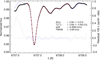 |
Fig. C.1. The best fitting 1D LTE LHD spectrum (red dashed line) superimposed on the solar flux spectrum of Kurucz (2005; black dots), fixing the continuum level at 0.9977 (relative to the continuum placement of the flux atlas), and using line list G09 with slight adjustments in the strengths of the CN, Fe, Si, and V lines (Case I, Table C.1) The right y-axis defines the scale of the residuals (thin blue line). |
Summary of the results of fitting the Li region of the solar flux spectrum (Kurucz 2005) with 1D LHD and 3D CO5BOLD synthetic spectra.
Next we fit the observed spectrum with a grid of synthetic spectra derived from the CO5BOLD 3D solar atmosphere, now treating the Li doublet in NLTE. Adopting the same continuum level as for the 1D fitting, we try out different assumptions about the chemical abundances and the wavelengths of the blend lines.
In Case Ia, we use the same line list (G09) as in Case I together with the same 1D-optimized individual abundances obtained from the best fit with the 1D LHD spectra. Under these constraints, the best fit requires A(Li) = 1.05 and q(Li) = 1.86%. As expected, the fit is rather poor (see Fig. C.2, top panel).
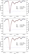 |
Fig. C.2. Best fits of the solar flux spectrum of Kurucz (2005; black dots) with different sets of 3D NLTE CO5BOLD spectra (red dashed line), adopting the same continuum level as in Fig. C.1. From top to bottom: Cases IIa, IIb, and IIc are all based on line list G09, but assume different chemical abundances and rest wavelengths of the blend lines (see text and Table C.1 for details). The right y-axis defines the scale of the residuals (thin blue line). |
At the next stage (Case Ib), we adjust the strengths of the CN, Fe, Si, and V blend lines according to the 3D–1D abundance corrections inferred from fitting the 3D synthetic line profiles of the individual blend lines by a grid of corresponding 1D spectra of different abundance, as described for the Li and Si lines in Appendix B. The fit with these adjusted abundances is shown in Fig. C.2 (middle panel), indicating A(Li) = 1.04 and a strongly negative 6Li/7Li of less than −2%. While the fit is generally improved with respect to Case Ia, the Fe+CN blend at λ 670.74 nm is by far not reproduced to the level of precision achieved with the 1D LHD fit (cf. Fig. C.1).
A 3D fit of comparable quality can be accomplished by readjusting the rest wavelengths of the main blend components according to their differential convective Doppler shifts. The latter are again deduced from fitting the synthetic 3D line profiles by their 1D counterparts, as described for the Li and Si lines in Appendix B. In Case Ic, we applied both these “theoretical” convective wavelength shifts and related abundance corrections to the CN, Fe, Si, and V blend lines. Indeed, the applied wavelength shifts3 lead to a dramatic improvement of the fit (see Fig. C.2), bottom panel). Now the best solution is found for A(Li) = 1.05 and q(Li) = −0.18%. We notice that the 6Li/7Li found from this fine-tuned 3D fit is now in very good agreement with the result from the LHD fit after application of the Δq3DNLTE−1DLTE correction (0.69 − 0.83 = −0.14%).
We performed the same exercise for a different continuum level, c1 = 0.9980 (Case II), which corresponds closely to the continuum placement adopted for the analysis of the PEPSI spectrum in Strassmeier et al. (2018). We verified (Case IIx) that we obtain very similar results when adopting their set of abundances: A(Li) = 1.09 and q(Li) = 1.77 ± 2.2%, compared to A(Li) = 1.09 and q(Li) = 1.44±1.6% in Strassmeier et al. (2018). Quantitatively, the two series of fits at slightly different continuum levels show a systematic offset in the absolute values of A(Li) and q(Li), but otherwise follow the same qualitative trends and lead to the same conclusions. Details of all fits discussed above can be found in Table C.1.
In summary, the fits of the solar spectrum by grids of 1D LHD and 3D CO5BOLD synthetic spectra computed with the full G09 line list justify our definition of the 3D NLTE corrections for A(Li) and q(Li) based on the comparison of 3D NLTE and 1D LTE Li-only line profiles. This conclusion is not limited to the solar case but should apply even more to the target stars of this paper, where a strong lithium feature dominates over relatively weak blend lines.
We chose the Sun for demonstration because all involved spectral lines are weak and therefore the combined spectrum may be constructed by linear superposition of the individual components. The presence of stronger lines would require a full spectrum synthesis of the complete spectrum for each individual configuration. Under these conditions, a fine-tuned 3D (NLTE) fit to the observed spectra of our target stars would be next to impossible. However, the exercise presented in this Appendix also strongly suggests that using 3D model spectra directly for the fitting is not really the most desirable approach since it requires non-trivial adjustments in the line lists that are fine-tuned by 1D methods.
All Tables
Summary of the results of fitting the Li region of the solar flux spectrum (Kurucz 2005) with 1D LHD and 3D CO5BOLD synthetic spectra.
All Figures
|
Fig. 1. The impact of the blending lines in the Li I λ670.8 nm region on the resulting 3D NLTE corrections. The best fitting 1D LTE spectrum (blue continuous line) is superimposed on the 3D NLTE spectrum (black dotted line) computed for Teff = 5870 K, log ℊ = 4.5, [Fe/H] = 0, A(Li)3DNLTE = 2.0, 6Li/7Li3DNLTE = 5% and representing the “observation”. The synthetic spectra are computed adopting only the Li I doublet including hyperfine structure (line list K95, upper panel), and the line list G09 (lower panel), which includes also other atomic blends. The right y-axis gives the scale of the residuals (blue dashed line). We measure A(Li) = 1.92 and 6Li/7Li = 6.1% for line list K95, and A(Li) = 1.92 and 6Li/7Li = 5.4% in case of line list G09. |
| In the text | |
|
Fig. 2. 3D NLTE corrections Δq3DNLTE−1DLTE (upper panels) and ΔA3DNLTE−1DLTE (lower panels) vs. Teff for [Fe/H] = 0, A(Li) = 2.0, q(Li) = 5%, obtained with line lists K95 (left panels) and G09 (right panels). The blue circles and the red triangles correspond to log ℊ = 4.0 and log ℊ = 4.5, respectively. The computed 3D NLTE corrections for different υ sin i values are connected with lines of different styles (see legend). |
| In the text | |
|
Fig. 3. Contour plots of 3D NLTE A(Li) corrections ΔA3DNLTE−1DLTE (upper panel) and 6Li/7Li corrections Δq3DNLTE−1DLTE (middle panel) in the Teff – [Fe/H] plane. The same 3D NLTE 6Li/7Li corrections in the Teff – log ℊ plane are shown in the bottom panel. The contours are computed for [Fe/H] = 0, ν sin i = 2km s−1, A(Li) = 2.0, and q(Li) = 5%, employing the analytical expressions in Eqs. (1) and (2) with the coefficients given in Table 2. |
| In the text | |
|
Fig. 4. Comparison of the 1D and 3D NLTE abundance corrections derived in this work with the 1D NLTE corrections from Lind et al. (2009; L2009, dotted lines) and Takeda & Kawanomoto (2005; T2005, dash-dotted lines) for metallicities −1.0, −0.5, 0.0, and +0.5 (from top left to bottom right). Red and blue triangles denote the individual 3D NLTE corrections, while red and blue circles denote the individual 1D NLTE corrections for A(Li) computed in this work (H2018) for log ℊ of 4.0 and 4.5, respectively. |
| In the text | |
|
Fig. 5. The best fitting 1D LTE spectrum (solid line) superimposed on the HARPS spectrum (dots) for HD 207129 (left panels) and HD 95456 (right panels). The synthetic line profiles are computed adopting the line lists G09, M12, and I14 (from top to bottom), with modifications described in Sect. 3.3. The right y-axis defines the scale of the residuals (dashed line). |
| In the text | |
|
Fig. 6. The best |
| In the text | |
|
Fig. 7. The best-fitting |
| In the text | |
|
Fig. 8. The best fitting 1D LTE ATLAS/MOOG spectrum (dashed line) superimposed on the solar flux atlas spectrum of Kurucz (2005; black dots), fixing the continuum level at 0.9977 (relative to the continuum placement of the flux atlas), and using line list G09 (with modifications described in Sect. 3.3) and slight adjustments in the strengths of the CN, Fe, Si, and V lines (see Case C, Table 6) The right y-axis defines the scale of the residuals (thin blue line). |
| In the text | |
|
Fig. A.1. 3D NLTE corrections for 6Li/7Li (left panel) and A(Li) (right panel) vs. Teff for [Fe/H] = −1.0, A(Li) = 2.0, q(Li) = 5%, derived with line list K95. The blue circles and the red triangles correspond to log ℊ = 4.0 and log ℊ = 4.5, respectively. The corrections for different υ sin i values are connected with lines of different styles. |
| In the text | |
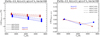 |
Fig. A.2. As Fig. A.1 but for [Fe/H] = 0.5. |
| In the text | |
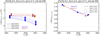 |
Fig. A.3. As Fig. A.1 but for [Fe/H] = +0.5. |
| In the text | |
|
Fig. A.4. Same corrections as shown in Figs. A.1–A.3, but derived with line list M12 for [Fe/H] = 0.0. |
| In the text | |
|
Fig. B.1. Best 1D fits (dashed line) to the 3D composite 7Li (NLTE) + Si (LTE) synthetic solar line profile (black solid line) achieved with different grids of 1D LTE 6Li + 7Li+Si profiles. From top to bottom: cases 2a, 2b, and 2c (see text and Table B.1 for details). The right y-axis defines the scale of the residuals (thin blue line). |
| In the text | |
|
Fig. C.1. The best fitting 1D LTE LHD spectrum (red dashed line) superimposed on the solar flux spectrum of Kurucz (2005; black dots), fixing the continuum level at 0.9977 (relative to the continuum placement of the flux atlas), and using line list G09 with slight adjustments in the strengths of the CN, Fe, Si, and V lines (Case I, Table C.1) The right y-axis defines the scale of the residuals (thin blue line). |
| In the text | |
|
Fig. C.2. Best fits of the solar flux spectrum of Kurucz (2005; black dots) with different sets of 3D NLTE CO5BOLD spectra (red dashed line), adopting the same continuum level as in Fig. C.1. From top to bottom: Cases IIa, IIb, and IIc are all based on line list G09, but assume different chemical abundances and rest wavelengths of the blend lines (see text and Table C.1 for details). The right y-axis defines the scale of the residuals (thin blue line). |
| In the text | |
Current usage metrics show cumulative count of Article Views (full-text article views including HTML views, PDF and ePub downloads, according to the available data) and Abstracts Views on Vision4Press platform.
Data correspond to usage on the plateform after 2015. The current usage metrics is available 48-96 hours after online publication and is updated daily on week days.
Initial download of the metrics may take a while.