| Issue |
A&A
Volume 615, July 2018
|
|
|---|---|---|
| Article Number | A162 | |
| Number of page(s) | 12 | |
| Section | Cosmology (including clusters of galaxies) | |
| DOI | https://doi.org/10.1051/0004-6361/201832932 | |
| Published online | 01 August 2018 | |
Correcting for peculiar velocities of Type Ia supernovae in clusters of galaxies
1
Université Clermont Auvergne,
CNRS/IN2P3,
Laboratoire de Physique de Clermont,
63000
Clermont-Ferrand,
France
e-mail: This email address is being protected from spambots. You need JavaScript enabled to view it.
2
Kavli Institute for Particle Astrophysics and Cosmology, Department of Physics, Stanford University,
Stanford,
CA
94305,
USA
3
Lomonosov Moscow State University, Sternberg Astronomical Institute,
Universitetsky pr. 13,
Moscow
119234,
Russia
4
Physics Division, Lawrence Berkeley National Laboratory,
1 Cyclotron Road,
Berkeley,
CA
94720,
USA
5
Laboratoire de Physique Nucléaire et des Hautes Énergies,
Université Pierre et Marie Curie Paris 6, Université Paris Diderot Paris 7, CNRS-IN2P3,
4 place Jussieu,
75252
Paris Cedex 05,
France
6
Department of Physics, Yale University,
New Haven,
CT
06250-8121,
USA
7
Department of Physics, University of California Berkeley,
366 LeConte Hall MC 7300,
Berkeley,
CA
94720-7300,
USA
8
Université de Lyon, Université de Lyon 1, Villeurbanne, CNRS/IN2P3, Institut de Physique Nucléaire de Lyon,
69622
Lyon,
France
9
Department of Physics and Astronomy, University of Southampton,
Southampton,
Hampshire
SO17 1BJ,
UK
10
The Oskar Klein Centre, Department of Physics, AlbaNova, Stockholm University,
106 91
Stockholm,
Sweden
11
Aix-Marseille Université, CNRS/IN2P3, CPPM UMR 7346,
13288
Marseille,
France
12
Max-Planck Institut für Astrophysik,
Karl-Schwarzschild-Str. 1,
85748
Garching,
Germany
13
Las Cumbres Observatory Global Telescope Network,
6740 Cortona Dr., Suite 102 Goleta,
CA 93117,
USA
14
Department of Physics, University of California,
Santa Barbara,
CA
93106-9530,
USA
15
Institut fũr Physik, Humboldt-Universitãt zu Berlin,
Newtonstr. 15,
12489
Berlin,
Germany
16
Deutsches Elektronen-Synchrotron,
15735
Zeuthen,
Germany
17
Tsinghua Center for Astrophysics, Tsinghua University,
Beijing
100084,
PR China
18
Centre de Recherche Astronomique de Lyon, Université Lyon 1,
9 Avenue Charles André,
69561
Saint-Genis-Laval,
France
19
Space Telescope Science Institute,
3700 San Martin Drive,
Baltimore,
MD
21218,
USA
20
European Southern Observatory,
Karl-Schwarzschild-Str. 2,
85748
Garching,
Germany
21
Computational Cosmology Center, Computational Research Division, Lawrence Berkeley National Laboratory,
1 Cyclotron Road MS 50B-4206,
Berkeley,
CA
94720,
USA
22
Kavli Institute for the Physics and Mathematics of the Universe, University of Tokyo,
5-1-5 Kashiwanoha,
Kashiwa,
Chiba
277-8583,
Japan
Received:
1
March
2018
Accepted:
6
April
2018
Abstract
Context. Type Ia supernovae (SNe Ia) are widely used to measure the expansion of the Universe. To perform such measurements the luminosity and cosmological redshift (z) of the SNe Ia have to be determined. The uncertainty on z includes an unknown peculiar velocity, which can be very large for SNe Ia in the virialized cores of massive clusters.
Aims. We determine which SNe Ia exploded in galaxy clusters using 145 SNe Ia from the Nearby Supernova Factory. We then study how the correction for peculiar velocities of host galaxies inside the clusters improves the Hubble residuals.
Methods. We found 11 candidates for membership in clusters. We applied the biweight technique to estimate the redshift of a cluster. Then, we used the galaxy cluster redshift instead of the host galaxy redshift to construct the Hubble diagram.
Results. For SNe Ia inside galaxy clusters, the dispersion around the Hubble diagram when peculiar velocities are taken into account is smaller compared with a case without peculiar velocity correction, which has a wRMS = 0.130 ± 0.038 mag instead of wRMS = 0.137 ± 0.036 mag. The significance of this improvement is 3.58σ. If we remove the very nearby Virgo cluster member SN2006X (z < 0.01) from the analysis, the significance decreases to 1.34σ. The peculiar velocity correction is found to be highest for the SNe Ia hosted by blue spiral galaxies. Those SNe Ia have high local specific star formation rates and smaller stellar masses, which is seemingly counter to what might be expected given the heavy concentration of old, massive elliptical galaxies in clusters.
Conclusions. As expected, the Hubble residuals of SNe Ia associated with massive galaxy clusters improve when the cluster redshift is taken as the cosmological redshift of the supernova. This fact has to be taken into account in future cosmological analyses in order to achieve higher accuracy for cosmological redshift measurements. We provide an approach to do so.
Key words: supernovae: general / galaxies: clusters: general / galaxies: distances and redshifts / dark energy
© ESO 2018
 Open Access article, published by EDP Sciences, under the terms of the Creative Commons Attribution License (http://creativecommons.org/licenses/by/4.0;), which permits unrestricted use, distribution, and reproduction in any medium, provided the original work is properly cited.
1 Introduction
Type Ia supernovae (SNe Ia) are excellent distance indicators. Observations of distant SNe Ia led to the discovery of the accelerating expansion of the Universe (Perlmutter et al. 1998, 1999; Riess et al. 1998; Schmidt et al. 1998). The most recent analysis of SNe Ia indicates that for a flat Λ CDM cosmology, our Universe is accelerating;this analysis found that ΩΛ = 0.705 ± 0.034 (Betoule et al. 2014; Scolnic et al. 2017).
Cosmological parameters are estimated from the luminosity distance-redshift relation of SNe Ia, using the Hubble diagram. Generally, particular attention is paid to standardization of SNe Ia, that is, to increase of the accuracy of luminosity distance determinations (Rust 1974; Pskovskii 1977, 1984; Phillips 1993; Phillips et al. 1999; Hamuy et al. 1996a; Riess et al. 1996; Perlmutter et al. 1997, 1999; Wang et al. 2003, 2009; Guy et al. 2005, 2007; Jha et al. 2007; Bailey et al. 2009; Kelly et al. 2010; Chotard et al. 2011; Blondin et al. 2012; Rigault et al. 2013; Kim et al. 2013; Fakhouri et al. 2015; Sasdelli et al. 2016; Léget 2016; Saunders 2017, in prep.). The uncertainty on the redshift is very often considered negligible. The redshift used in the luminosity distance-redshift relation is due to the expansion of the Universe assuming Friedman–Lemaitre–Robertson–Walker metric, that is, the motion within the reference frame defined by the cosmic microwave background radiation (CMB). We refer to this as a cosmological redshift (zc). In fact, the redshift observed on the Earth (zobs) also includes the contribution from the Doppler effect induced by radial peculiar velocities (zp),
 (1)
(1)
At low redshift and for low velocities compared to the speed of light in vacuum, the following approximation can be used:
 (2)
(2)
The component of the redshift due to peculiar velocities includes the rotational and orbital motions of the Earth, the solar orbit within the Galaxy, peculiar motion of the Galaxy within the Local Group, infall of the Local Group toward the center of the Local Supercluster, etc. It is well known that peculiar velocities of SNe Ia introduce additional errors to the Hubble diagram and therefore have an impact on the estimation of cosmological parameters (Cooray & Caldwell 2006; Hui & Greene 2006; Davis et al. 2011; Habibi et al. 2018). To minimize the influence of poorly constrained peculiar velocities, in some cosmological analyses all SNe Ia with z < 0.015 are removed from the Hubble diagram fitting and a 300–400 km s−1 peculiar velocity dispersion is added in quadrature to the redshift uncertainty (Astier et al. 2006; Wood-Vasey et al. 2007; Amanullah et al. 2010). In particular, this is the approach taken for the cosmology analysis using Union 2.1 (Suzuki et al. 2012). Another way to apply the peculiar velocity correction is to measure the local velocity field assuming linear perturbation theory and then correct each supernova redshift (Hudson et al. 2004). Willick & Strauss (1998) estimated the accuracy of this method to be ~100 km s−1, Riess et al. (1997) adopted the value of 200 km s−1, and Conley et al. (2011) used 150 km s−1. This approach was used in the Joint Light-Curve Analysis (JLA; Betoule et al. 2014). However, it has been shown that the systematic uncertainty on w, the dark energy equation of state parameter, of different flow models is at the level of ±0.04 (Neill & Conley 2007).
It has nonetheless been observed that velocity dispersions can exceed 1000 km s−1 in galaxy clusters (Ruel et al. 2014). For example, in the Coma cluster, a large cluster of galaxies that contains more than 1000 members, the velocity dispersion isσV = 1038 km s−1 (Colless & Dunn 1996). The dispersion inside the cluster can be much greater than that usually assumed in cosmological analyses and therefore can seriously affect the redshift measurements (see Fig. 1). Moreover, within a cluster, the perturbations are no longer linear, and therefore cannot be corrected using the smoothed velocity field. Assuming a linear Hubble flow, we can transform the dispersion due to peculiar velocities into the following magnitude error:
 (3)
(3)
Calculations using Eq. (3) show that for the low redshift region (z < 0.05) this error is higher than the 150 and 300 km s−1 that is usually assumed and is two times larger than the intrinsic dispersion of SNe Ia around the Hubble diagram (Fig. 2). This means that standard methods to take into account peculiar velocities do not work for galaxies inside clusters, and another more accurate method needs to be developed for these special cases.
For a supernova (SN) in a cluster it is possible to estimate zc more accurately using the host galaxy cluster redshift (zcl) instead of the host redshift1 (zhost). The mean cluster redshift is not affected by virialization within a cluster. Of course, clusters also have peculiar velocities that can sometimes manifest themselves as cluster merging, for example, Bullet clusters (Clowe et al. 2006). However, clusters have much smaller peculiar velocities than the galaxies within them (i.e., ~300 km s−1; Bahcall & Oh 1996; Dale et al. 1999; Masters et al. 2006).
The fact that there is additional velocity dispersion of galaxies inside the clusters that should be taken into account has been known for a long time. Indeed, the distance measurements are degenerate in terms of redshift due to the presence of galaxy clusters and this is accounted for when Tully–Fisher method (Tully & Fisher 1977) is applied to measure distances. This problem is known as the triple value problem, which is the fact that for a given distance one can get three different values of redshift due to the presence of a cluster (see, e.g., Tonry & Davis 1981; Tully & Shaya 1984; Blakeslee et al. 1999; Radburn-Smith et al. 2004; Karachentsev et al. 2014). To account for the peculiar velocities of galaxies in clusters, Blakeslee et al. (1999) proposed several alternative approaches. The first is to keep using the individual velocities of galaxies but to add extra variance in quadrature for the clusters according to ![Mathematical equation: $\sigma_{cl}(r)=\sigma_0/[1+(r/r_0)^2]^{1/2}$](/articles/aa/full_html/2018/07/aa32932-18/aa32932-18-eq4.png) , where σ0 = 700 (400) km s−1 and r0 = 2 (1) Mpc for Virgo (Fornax). The second approach is to use a fixed velocity error and to remove the virial dispersion by assigning galaxies their group-averaged velocities. Nevertheless, peculiar velocity correction within galaxy clusters has received little attention in SN Ia studies, with the exceptions of Feindt et al. (2013) and Dhawan et al. (2018). The redshift correction induced by galaxy clusters is mentioned only briefly in those analyses, as their objectives were to measure the bulk flow with SNe Ia (Feindt et al. 2013) and the Hubble constant (Dhawan et al. 2018). However, at low redshifts this correction is necessary, which is why we focus on it here.
, where σ0 = 700 (400) km s−1 and r0 = 2 (1) Mpc for Virgo (Fornax). The second approach is to use a fixed velocity error and to remove the virial dispersion by assigning galaxies their group-averaged velocities. Nevertheless, peculiar velocity correction within galaxy clusters has received little attention in SN Ia studies, with the exceptions of Feindt et al. (2013) and Dhawan et al. (2018). The redshift correction induced by galaxy clusters is mentioned only briefly in those analyses, as their objectives were to measure the bulk flow with SNe Ia (Feindt et al. 2013) and the Hubble constant (Dhawan et al. 2018). However, at low redshifts this correction is necessary, which is why we focus on it here.
In this paper we identify SNe Ia that appear to reside in known clusters of galaxies. We then estimate the impact of their peculiar velocities by replacing the host redshift by the cluster redshift. As our parent sample we use 145 SNe Ia observed by the Nearby Supernova Factory (SNFACTORY), a project devoted to the study of SNe Ia in the nearby Hubble flow (0.02 < z < 0.08; Aldering et al. 2002). We then compare the Hubble residuals (HRs) for SNe Ia in galaxy clusters before and after peculiar velocity correction.
The paper is organized as follows. In Sect. 2, the SNFACTORY dataset is described. In Sect. 3 the host clusters data and the matching with SNe Ia are presented. In Sect. 4 we introduce the peculiar velocity correction and study how it affects the HRs. We discuss the robustness of our results and the properties of SNe Ia in galaxy clusters in Sect. 5. Finally, the conclusions of this study are given in Sect. 6.
Throughout this paper, we assume a flat ΛCDM cosmology with ΩΛ = 0.7, Ωm = 0.3, and H0 = 70 km s−1 Mpc−1. Varying these assumptions has negligible impact on our results due to the low redshifts of our SNe Ia and the fact that H0 is simply absorbed into the Hubble diagram zero point.
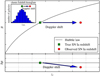 |
Fig. 1 Hubble diagram demonstrating how large peculiar velocity can affect the measurements of the expansion history of the Universe. The inset plot is a typical velocity distribution of galaxies inside a cluster. |
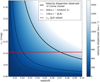 |
Fig. 2 Redshift uncertainties (in magnitude units) due to different levels of peculiar velocities as a function of the cosmological redshift. The solid black line corresponds to the Coma cluster velocity dispersion; the dashed and dash-dotted lines correspond to 300 and 150 km s−1, respectively. The red line shows the intrinsic dispersion of SNe Ia on the Hubble diagram found for the JLA sample (Betoule et al. 2014). |
2 Nearby Supernova Factory data
This analysis is based on 145 SNe Ia obtained by the SNFACTORY collaboration between 2004 and 2009 with the SuperNova Integral Field Spectrograph (SNIFS; Aldering et al. 2002; Lantz et al. 2004) installed on the University of Hawaii 2.2 m telescope (Mauna Kea). The SNIFS is a fully integrated instrument optimized for semi-automated observations of point sources on a structured background over an extended optical window at moderate spectral resolution. This instrument has a fully filled 6.4″ ×6.4″ spectroscopic field of view subdivided into a grid of 15 × 15 contiguous square spatial elements (spaxels). The dual-channel spectrograph simultaneously covers 3200–5200 Å (B-channel) and 5100–10 000 Å (R-channel) with 2.8 and 3.2 Åresolution, respectively. The data reduction of the x, y, λ data cubes was summarized by Aldering et al. (2006) and updated in Sect. 2.1 of Scalzo et al. (2010). A preview of the flux calibration is developed in Sect. 2.2 of Pereira et al. (2013), based on the atmospheric extinction derived in Buton et al. (2013), and the host subtraction is described in Bongard et al. (2011). For every SN followed, the SNFACTORY creates a spectrophotometric time series composed of ~13 epochs on average; the first spectrum was taken before maximum light in the B-band (Bailey et al. 2009; Chotard et al. 2011). In addition, observations are obtained at the supernova location at least one year after the explosion to serve as a final reference to enable the subtraction of the underlying host. The host galaxy redshifts of the SNFACTORYSNe Ia are given in Childress et al. (2013). The sample of 145 SNe Ia contains those objects through 2009 having good final references and properly measured light curve parameters, including quality cuts suggested by Guy et al. (2010).
The nearby supernova search is more complicated than the search for distant SNe Ia because to probe the same volume it is necessary tosweep a much larger sky field. Rather than targeting high-density galaxy fields that could potentially bias the survey, at the beginning of the SNFACTORY experiment (2004–2008) SNe Ia were discovered with the 1.2 m telescope at the Mount Palomar Observatory(Rabinowitz et al. 2003) in a nontargeted mode, by surveying about 500 square degrees of sky every night. In all ~20 000 square degrees were monitored over the course of a year. The SNFACTORY performed follow-up observations of a few SNe Ia discovered by the Palomar Transient Factory (Law et al. 2009), which also were found in a nontargeted search. We chose to examine this sample, despite it being only 20% of all nearby cosmologically useful SNe Ia in order to use a homogeneous dataset primarily from a blind SN Ia search to avoid any bias due to the survey strategy. However, 22 SNe Ia in the sample were not discovered by these research programs but by amateur astronomers or specific surveys in clusters of galaxies. In particular, SN2007nq, which will be identified as being in a cluster, comes from a specific search within clusters of galaxies (Quimby et al. 2007); SN2006X and SN2009hi, which were also identified as being in clusters, come from targeted searches (Suzuki & Migliardi 2006; Nakano et al. 2009).
As mentioned above, SN2006X is located in the Virgo cluster and is a highly reddened SN Ia with a SALT2 color of C = 1.2. This SN Ia would not be kept for a classical cosmological analysis, but since we are only interested in the effects of peculiar velocities, we have kept it in the analysis.
3 Host clusters data
In this section we describe how we selected the cluster candidates for associations with SNFACTORY SNe (Sect. 3.1). We then present our technique for calculating the cluster redshift and its error (Sect. 3.2). Our final list of associations appears in Sect. 3.3.
3.1 Preliminary cluster selection
Several methods for identifying clusters of galaxies have been developed (e.g., Abell 1958; Zwicky et al. 1961; Gunn et al. 1986; Abell et al. 1989; Vikhlinin et al. 1998; Kepner et al. 1999; Gladders & Yee 2000; Piffaretti et al. 2011; Planck Collaboration XXIV 2016). However, each of these methods contains assumptions about cluster properties and is subject to selection effects. The earliest method used to identify clusters was the analysis of the optical images for the presence of over-density regions. Finding clusters with this method suffers from contamination by foreground and background galaxies that produce the false effect of over-density, which becomes more significant for high redshift. The method that helps to reduce this projection effect is the red sequence method (RSM). This method is based on the fact that galaxy clusters contain a population of elliptical and lenticular galaxies that follow an empirical relationship between their color and magnitude and form the so-called red sequence (Gladders & Yee 2000). The projection of random galaxies at different redshifts is not expected to form a clear red sequence. The RSM also requires multicolor observations. Spectroscopic redshift measurements help tremendously in establishing which galaxies are cluster members, although even then the triple value problem can lead to erroneous associations.
A third popular and effective method to detect galaxy clusters is to observe the diffuse X-ray emission radiated by the hot gas (106 –108 K) in the centers of the clusters (Boldt et al. 1966; Sarazin 1988). In virialized systems the thermal velocity of gas and the velocity of the galaxies in the cluster are determined by the same gravitational potential. As a result, clusters of galaxies where peculiar velocities are important appear as luminous X-ray emitters and have typical luminosities of  1043 – 1045 erg s−1. Such luminosities correspond to σV ≳ 700 km s−1 (see Fig. 3). The gas distribution can be rather compact and thus unresolved by X-ray surveys at intermediate and high redshifts. However, nearby clusters (z < 0.1) are well resolved, eliminating contamination from X-ray AGN or stars.
Finally, clusters of galaxies also cause distortions in the CMB from the inverse Compton scattering of the CMB photons by the hot intra-cluster gas. In the fourth and final cluster identification method, this signature, known as the Sunyaev-Zel’dovich (SZ) effect, is used to identify clusters (Planck Collaboration XXIV 2016).
Using the SIMBAD database (Wenger et al. 2000), we chose all the clusters projected within ~2.5 Mpc around the SNe Ia positions and with redshift differing from that of the supernova by less than 0.015. SN Ia host redshifts were used to initially determine the distance. We did not consider objects classified as groups of galaxies (GrG), although there is no strong boundary between these and clusters since GrG are characterized by smaller mass and therefore smaller velocity dispersion ~300 km s−1 (see Fig. 5 in Mulchaey 2000). The uncertainty introduced by such velocity is properly accounted for using the conventional method of assigning a fixed uncertainty to all SNe Ia to account for peculiar velocities.
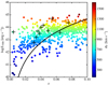 |
Fig. 3 Luminosities of [0.1–2.4 keV] within R500 of MCXC clusters (Piffaretti et al. 2011) as a function of redshift, up to z = 0.1. The colorbarshows the corresponding cluster velocity dispersion σV calculated from Eq. (7). Black plus signs indicate clusters from the current analysis. The black curve corresponds to the intrinsic dispersion of SNe Ia on the Hubble diagram found for the JLA sample (Betoule et al. 2014) projected onto cluster luminosities by combining the luminosity–mass and mass–velocity dispersion relations. |
3.2 Cluster redshift measurement
Some published cluster redshifts have been determined from a single or few galaxies. As we want to have a precise redshift correction, we cannot simply replace the redshift of the host galaxy by the redshift of another galaxy. We therefore adopt the following method to improve cluster redshift estimates.
To measure the redshift of the cluster, it is necessary to know which galaxies in the cluster field are its members. Galaxy clusters considered in this paper are old enough (z < 0.1) to exhibit virialized regions (Wu et al. 2013). Therefore, to characterize the cluster radius we used the virial radius R200, corresponding to an average enclosed density equal to 200 times the critical density of the Universe at redshift z, as follows:
 (4)
(4)
 (5)
(5)
where H(z) is the Hubble parameter at redshift z and G is the Newtonian gravitational constant.
According to the virial theorem, the velocity dispersion σV inside a cluster is given as
 (6)
(6)
Using Eq. (5) and  , we find
 (7)
(7)
The cluster redshift uncertainty ( ) can be found from the cluster velocity dispersion and is written as
 (8)
(8)
where Ngal is a number of cluster members used for the calculation.
First, we took all the galaxies attributed to each cluster in literature sources and added the SNFACTORY host galaxy if it was not among them. Then, these data were combined with the Data Release 13 of the release database of the Sloan Digital Sky Survey (SDSS; Eisenstein et al. 2011; Dawson et al. 2013; Smee et al. 2013; SDSS Collaboration 2017). We selected all galaxies with spectroscopic redshifts located in a circle with the center corresponding to the cluster coordinates and projected inside the R200 radius of the cluster. A 5σV redshift cut was adopted in the redshift direction (see Eq. (7)).
The R200 value was extracted from the literature when possible. For the clusters without published size measurements we estimated R200 ourselves from the velocity distribution of galaxies around the cluster position following the procedure described in Beers et al. (1990) with an initial guess of R200 = 1.1 Mpc. If the number of cluster members with spectroscopically determined redshifts was less than ten, the value of 1.1 Mpc was adopted as a virial radius. This value corresponds to the average R200 of clusters in the Meta-Catalog of X-Ray Detected Clusters of Galaxies (MCXC; Piffaretti et al. 2011); see Fig. 3.
To estimate the redshift of a cluster we applied the so-called biweight technique (Beers et al. 1990) on the remaining redshift distributions. Biweight determines the kinematic properties of galaxy clusters while being resistant to the presence of outliers and is robust fora broad range of underlying velocity distributions, even if they are non-Gaussian, using the median and an outlier rejection based on the median absolute deviation. Moreover, Beers et al. (1990) provided a formula for the cluster redshift uncertainty, but it cannot be used for clusters with few members. Therefore, instead we used Eq. (8), which can be applied for all of our clusters.
For some of the clusters the literature provides only the final redshift and the number of galaxies, Npaper, that were used in the calculation, without publishing a list of cluster members. In those cases, if the number of members collected by us satisfies Ngal < Npaper we adopted the redshift from literature. The detailed scheme of the cluster redshift calculation is presented in Fig. 4.
All the calculations described above are based on spectroscopical redshifts. Before performing the calculations of the cluster CMB redshift, all of the heliocentric redshifts of its members were first transformed to the CMB frame. The transformation to the CMB frame made use of the NASA/IPAC Extragalactic Database (NED).
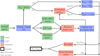 |
Fig. 4 Workflow for redshift calculation and other inputs for matching of SNe to galaxy clusters. In this scheme, Ngal corresponds to the number of galaxies used to compute the redshift and Npaper corresponds to the number of galaxies used to estimate the redshift in the literature. |
3.3 Finalmatching and confirmation
Once the redshifts and R200 values were obtained for each cluster, we performed the final matching. A supernova is considered a cluster member if the following two conditions are satisfied:
-
r < R200, where r is the projected distance between the SN and cluster center.
-
 .
.
The SNe Ia that did not satisfy these criteria were removed from further consideration.
Our final criteria are slightly different than those applied by Xavier et al. (2013) (1.5 Mpc and σV = 500 km s−1) and Dilday et al. 2010 (1 Mpc h−1 and Δz = 0.015). These authors studied the properties and rate of supernovae in clusters and their choices were made to be consistent with previous cluster SN Ia rate measurements. These values roughly characterize an average cluster and we were guided by the same thoughts when making the preliminary cluster selection (2.5 Mpc and Δ z = 0.015, see Sect. 3.1). However, since clusters have different size and velocity dispersion, we determined or extracted from the literature the physical parameters of each cluster (R200 and σV). This method provides an individual approach to each SN-cluster pair and allows association with a cluster to be defined with greater accuracy.
Following Carlberg et al. (1997), and Rines & Diaferio (2006), we constructed an ensemble cluster from all the clusters associated with SNe Ia to smooth over the asymmetries in the individual clusters. We scaled the velocities by σV and positions with the values of R200 for each cluster to produce Fig. 5. This shows our selection boundaries and exhibits good separation of cluster galaxies from surrounding galaxies.
As it was mentioned in Sect. 3.1 there are several methods to identify a cluster. Initially we considered everything that is classified as a cluster by previous studies. However, some of these classifications can be false. For the remaining clusters we checked for the presence of X-ray emission, a red sequence, or the SZ effect, as described below.
We used the public ROSAT All Sky Survey images within the energy band 0.1–2.4 keV to look for extended X-ray counterparts2. The expected [0.1–2.4 keV] luminosity within R500 can be extracted from the luminosity–mass relation  with log(C) = 0.274 and α =1.64 (see Table 1 in Arnaud et al. 2010). The L500 values for MCXC clusters (Piffaretti et al. 2011) as a function of redshift are presented in Fig. 3. Moreover, in Fig. 3 a continuous black line represents the minimum value of L500 that is required for the velocity dispersion of the cluster to cause a deviation from the Hubble diagram greater than the intrinsic dispersion in luminosity of SNe Ia. The figure shows that all the clusters hosting SNe Ia except one are above this threshold and it is therefore very likely that the Doppler effect induced by these clusters causes a dispersion in the Hubble diagram that is greater thanthe intrinsic dispersion in luminosity of SNe Ia. Moreover, more than a half of the low redshift clusters are above this limit, indicating that the peculiar velocity correction has to be taken into account if a SN Ia belongs to a cluster of galaxies and is observed at low redshift.
To check for a linear red sequence feature, SDSS data were employed. From the SDSS Galaxy table we chose all the galaxies in the R200 region around the cluster position. We extracted model magnitudes, as recommended by SDSS for measuring colors of extended objects.
We checked for detections of the SZ effect using the Planck catalog of Sunyaev-Zel’dovich sources (Planck Collaboration XXVII 2016). All the clusters in our sample with SZ sources also have X-ray emission, as expected for real clusters.
Some ofour supposed clusters do not show X-ray or SZ signatures of a cluster. As described in Sect. 3.1, low redshift clusters are expected to have X-ray emission. Therefore, only such candidates were kept for further analysis (see Fig. 3).
Cases in which the red sequence is clearly seen but for which there is no diffuse X-ray emission can be explained either by the superposition of nearby clusters or being a group embedded in a filament. For example, our study of the redshift distribution and sky projection around the proposed host cluster [WHL2012] J132045.4+211627 of SNF20070417-002 revealed that many of the redshifts used to determine zcl come from galaxies that are more spread out – like a filament would be. We conclude that, consistent with the lack of X-rays, this is not a cluster.
Two other clusters, ZwCl 2259+0746 and A87, also require discussion. Within 2.3′ of the center of ZwCl 2259+0746 there is a source of X-ray emission, 1RXS J230215.3+080159. However, the size of the emission region (3′) is very small in comparison with R500 value for the cluster (40′). In addition, according to Mickaelian et al. (2006), this emission belongs to a star. Therefore, we did not assign this X-ray source to ZwCl 2259+0746. Another case is A87, which belongs to the A85/87/89 complex of clusters of galaxies. According to Durret et al. (1998), the galaxy velocities in the A87 region show the existence of subgroups, which all have an X-ray counterpart and seem to be falling onto A85 along a filament. Therefore, A87 is not really a cluster but a substructure of A85 that has a very prominent diffuse X-ray emission (Piffaretti et al. 2011). We applied our redshift measurement technique to determine the CMB redshift of the virialized region of A85. Thus, we included A85/A87 in our final table for the peculiar velocity analysis.
The final list of SNFACTORY SNe Ia in confirmed clusters contains 11 objects. The resulting association of SNe Ia with host clusters is given in Table 1. Column 1 is the SN name, Col. 2 contains a name of the identified host cluster of galaxies, and Col. 3 is the MCXC name. The MCXC coordinates of the host cluster center are given in Col. 4. Column 5 contains the projected separation, D, in Mpc between the SN position and the host cluster center. The R200 value is in Col. 6 and the CMB supernova redshift is in Col. 7. The CMB redshift of the cluster and its uncertainty can be found in Cols. 8 and 9. The velocity dispersion of the cluster estimated from the R200 value is shown in Col. 10. The number of galaxies that were used for cluster redshift calculation is in Col. 11. In Col. 12 we indicate the source of galaxy redshift information (lit. is an abbreviation for literature). In the last Col., we summarize all references for the cluster coordinates, R200, and non-SN galaxy redshifts.
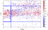 |
Fig. 5 Speed normalized by velocity dispersion within the ensemble cluster vs. the distance between galaxies and ensemble cluster normalized by R200. The small points indicate galaxies with spectroscopy from SDSS. The big points represent the positions of host galaxies of our SNe Ia. The color bar shows the corresponding g− r color; the points filled with gray do not have color measurements. The solid lines show the cuts we applied to associate SNe Ia withclusters, and the dashed lines represent the prolongation of those cuts. |
Association of the SNFACTORY SNe Ia with host clusters.
4 Impacton the Hubble diagram
Since we have a list of 11 SNe Ia that belong to clusters, we can apply peculiar velocity corrections and study how they affect the HRs. The following method is implemented.
The theoretical distance modulus is μth = 5log10dL − 5, where dL is the true luminosity distance in parsecs, and
 (9)
(9)
where zh is the heliocentric redshift, which takes into account the fact that the observed flux is affected not only by the cosmological redshift but by the Doppler effect as well.
We assign the cosmological redshift zc to be
 (10)
(10)
The uncertainty on zc (both SN Ia and host cluster) is propagated into the magnitude error  as
as
 (11)
(11)
where  is the propagation of uncertainty from light curve parameters to an apparent magnitude of SN Ia in the B-band, and
  , σint is the unknown intrinsic dispersion ofSN Ia. The value σz is the uncertainty on redshift measurement and peculiar velocity correction (see Eq. (3)), which is assigned as
 (12)
(12)
The 0.001 value corresponds to the 300 km s−1 that is added to the redshift error of SNe Ia outside the clusters to take into account the unknown galaxy peculiar velocities, as in a classical cosmological analysis. For cases in which a SN Ia belongs to a galaxy cluster, we assume that the redshift error contains only the error from the redshift measurement of a cluster.
By fitting the Hubble diagram using only SNe Ia outside the galaxy clusters3, we obtained SN Ia SALT2 nuisance parameters: α and β, the classical standardization parameters for light curve width and color, respectively; and the absolute magnitude MB, and intrinsic dispersion. These nuisance parameters remained fixed during our analysis. Once the nuisance parameters were estimated, we computed the difference between observed and theoretical distance modulus (HRs). In order to study the impact of peculiar velocity correction, we computed the HRs for the SNe Ia in clusters before and after correction. We used the weighted root mean square (wRMS) as defined in Blondin et al. 2011 to measure the impact of this correction. We used the same intrinsic dispersion established during the fitting (σint = 0.10 mag) to calculate all wRMS. SN2006X was not taken into account during the computation of the wRMS because it does not belong to the set of so-called normal SNe Ia. However, SN2006X is included in the statistical tests described below (for details see Sect. 5.1).
The dispersion of these 11 SNe Ia around the Hubble diagram decreases significantly when the peculiar velocities of their hosts inside the clusters are taken into account (wRMS = 0.130 ± 0.038 mag). When using the redshift of the host instead of the redshift of the cluster, the dispersion of these 11 SNe Ia is wRMS = 0.137 ± 0.036 mag (see Fig. 6). In order to compute the significance of this improvement, the Pearson correlation coefficient and its significance between HR before the correction and 5 log10(zcl∕zhost) are computed. The Pearson correlation coefficient is ρ = 0.9 ± 0.1, and its significance is 3.58σ, which is significant. In order to cross-check this significance, we did a Monte Carlo simulation. For each simulation, we took the difference zcl − zhost for the 11 SNe Ia in clusters and then randomly applied these corrections to the same 11 SNe Ia. For each simulation, we examined how often we get a wRMS less than or equal to the observed wRMS after the fake random peculiar velocity correction. On average the wRMS is higher and the probability to have the same or lower dispersion in wRMS is 5.9 × 10⁻⁴, which is in agreement with Pearson correlation significance.
Even though the p-value is low, we still need to clarify why the decrease in wRMS is not higher. In order to examine whether the corrections are consistent with what it is expected, we compute the distribution of the pull of peculiar velocities and the expected distribution of HRs of our correction. These two distributions are shown, respectively, in Figs. 7 and 8. For the pull distribution shown in Fig. 7, which is defined as the distribution of difference between the host galaxy redshift and the host galaxy clusters redshift, divided by the peculiar velocity dispersion within the cluster, we should expect to get a centered normal distribution with a standard deviation of unity. The standard deviation of the pull is 0.82± 0.18, which is consistent with the expected unity distribution of the pulls. In addition, we showed in Fig. 8 the expected distribution of the correction, the expected distribution of the correction convolved with uncertainties on HR, and the observed distribution of the correction. It is seen that the observed distribution of the corrections and the predicted distribution of the corrections are consistent.
To resume, the Pearson correlation coefficient and its significance, the distribution of the pull, and the comparison between the expected correction and observed correction show that our correction is consistent with expectations given the cluster velocity dispersions and uncertainty in SN Ia luminosity distance.
In addition, the wRMS we found for SNe Ia inside the clusters before correction, 0.137 ± 0.036 mag, is also smaller than the wRMS for the SNe Ia in the field (wRMS = 0.151 ± 0.010 mag). This is consistent with a statistical fluctuations, but could be owing to a lower intrinsic luminosity dispersion for SNe Ia inside galaxy clusters. This possibility is explored in the Sect. 5.2.
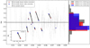 |
Fig. 6 Hubble diagram residuals. For cluster members red circles (blue squares) and histograms correspond to residuals for SNe Ia in galaxy clusters before (after) correction for peculiar velocities of the hosts inside their clusters. The black histogram corresponds to all SNe Ia after correction. SN2006X is presented in the inset plot separately from the others owing to its very large offset. |
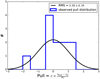 |
Fig. 7 Velocity pull distribution (in blue) in comparison with a Gaussian distribution with the observed standard distribution of the velocity pull. This is compatible with the expected standard deviation of unity. |
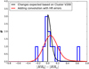 |
Fig. 8 Distribution of the difference in absolute HR after (HRa) and before (HRb) peculiar velocity correction (in blue). The black line represents the expected distribution of the difference in HR, and the red curve is the expected change convolved with error distribution. The results are compatible with the observed distribution given the Poisson uncertainties of each histogram bin. |
5 Discussion
5.1 SN2006X
Throughoutthe analysis, we treated SN2006X in a special way because this SN Ia is highly reddened SN, that is, it is associated with dusty local environment (Patat et al. 2007). This SN Ia affects the interstellar medium and exhibits very high ejecta velocities and a light echo (Patat et al. 2009). These special features put it very far off the Hubble diagram, and makes this SN unsuitable for cosmological analysis. However, it was included in the analysis because we are interested in the impact of peculiar velocities within galaxy clusters, not cosmology alone, and it passes the light curve quality criteria defined in Guy et al. (2010). While SN2006X can bias the dispersion, only the difference between the residuals before correction for peculiar velocity and after correction for peculiar velocity is taken into account in the computation of the significance of the signal. This correction for SN2006X is around ~550 km s−1 in velocity and has a huge impact on magnitude at nearby redshift. In this case the ~0.7 magnitude correction improves the dispersion on the Hubble diagram. Indeed, the original HR was measured as approximately − 1.7 mag when using the host galaxy redshift instead of the redshift of the galaxy cluster, whereas the HR is approximately − 1.0 mag. This correction is <50% of the original offset, and smaller than the corrected residual from stretch and color only.
Considering the importance of the correction for SN2006X and the fact that this object is peculiar, it makes sense to calculate the significance of the peculiar velocity correction when SN2006X is not taken into account. Without SN2006X, the Pearson correlation coefficient decreases substantially to ρ = 0.5 ± 0.3 with a signifcance of 1.34σ. Moreover, by carrying out the same Monte-Carlo simulation as in Sect. 4 for the remaining cluster SNe Ia, the P-value changes from 5.9 × 10⁻⁴ to 6.6 × 10⁻², which is in agreement with Pearson correlation significance. Thus, removing an object for which the correction is large decreases the significance of the correction, especially given the small sample size.
5.2 Physical properties of SNe Ia and their hosts in galaxy clusters
In Sect. 4 it was shown that the wRMS around the Hubble diagram for the SNe Ia in clusters is less than for SNe Ia in the field, which suggests that SNe Ia in clusters might represent a more “standard” subclass of SNe Ia (see Fig. 6). In order to compute the significance of this lower dispersion, we perform 106 Monte Carlo simulations. For each simulation, we randomly select 11 SNe Ia in our sample and compute the wRMS. For all the simulations we compute how often the dispersion is lower than the dispersion of wRMS = 0.130 ± 0.038 mag observed inside clusters after the peculiar velocity correction. In this case, the probability to have such a low dispersion is 3.8 × 10⁻¹, which is notsignificant.
Despite the low significance of their smaller dispersion, we could expect some difference between SNe Ia inside and outside clusters because the properties of the galaxies inside the clusters are known to be different from those in the field. While in the field all morphological types of the galaxies are observed, the central parts of the clusters usually contain a large percentage of elliptical galaxies. The oldest stars, with ages comparable to those of the Universe, lie in elliptical/lenticular galaxies. Moreover, dust is often absent in these regions. As shown by previous studies, narrow light curve SNe Ia are preferentially hosted by galaxies with little or no ongoing star formation, and usually occur in more massive galaxies (Hamuy et al. 1995, 1996b, 2000; Riess et al. 1999; Sullivan et al. 2003, 2006, 2010; Neill et al. 2009; Smith et al. 2012; Johansson et al. 2013; Hill et al. 2016; Henne et al. 2017). Indeed, if we examine Fig. 9, we see that 11 SNe Ia found in clusters are consistent with those studies, SNe Ia with higher X1 belong to the hosts with higher local specific star formation rate (sSFR) and smaller Mstellar. The properties of 48 SNe Ia in clusters versus 1015 SNe Ia in the field were studied in Xavier et al. (2013), who found the following mean values for SN LC parameters:  (field), − 0.40 ± 0.20 (clusters), and
  (field), and − 0.03 ± 0.02 (clusters). For comparison our means are
  (field), − 0.65 ± 0.36/ − 0.56 ± 0.34 (clusters without/with SN2006X), and
  (field), 0.02 ± 0.03/0.13 ± 0.11 (clusters without/with SN2006X). The correlation between HRs for 11 SNe in clusters and the mass of their host galaxy is the same as shown in Fig. 15 of Xavier et al. (2013).
We also performed a morphological classification of the hosts (see Table 2) based on the information provided by SIMBAD and HYPERLEDA databases (Wenger et al. 2000; Makarov et al. 2014) and images from Childress et al. (2013). The host of SNF20080612−003 is classified as elliptical by HYPERLEDA and as spiral by Sternberg et al. (2011). However, the classification by Sternberg et al. (2011) is based on images from Digital Sky Survey. This host looks elliptical without any sign of spiral arms on the SDSS image. Therefore, we assigned this galaxy to elliptical as in HYPERLEDA. We found that four SNe belong to elliptical/lenticular galaxies while the other seven are located in spirals. All of the early-type (elliptical and lenticular) galaxies fall on the red sequence for their clusters (see the color–magnitude diagrams (g− r vs. r) for the clusters within the SDSS footprint in Fig. 10). For the most part the spiral hosts are very close to the red sequence as well, that is, these galaxies are characterized by redder colors.
In Figs. 9 and 11 we also show how the peculiar velocity correction c|Δ z| and the absolute change in HRs due to peculiar velocity correction depend on the supernova parameters X1 and C, host properties such as local sSFR, stellar mass, morphological type, the difference between (g− r) of the host and corresponding (g−r) of the red sequence (RS residuals), relative SN position inside the cluster, and cluster mass M200 (Childress et al. 2013; Brown et al. 2014; Rigault et al. 2018). The c|Δz| plot shows that most of the SNe whose redshifts are significantly changed have X1 ≃ 0 and are hosted by blue spiral galaxies that have high local sSFR and smaller Mstellar, r∕R200 ≃ 0.7 (see Fig. 9). This is consistent with the distribution of galaxies in clusters such that the massive, elliptical, and passive galaxies are located in the center but outer region contains spiral galaxies as well and with velocity profiles inside the clusters (see Fig. 5; Carlberg et al. 1997, their Fig. 1; and Rines & Diaferio 2006, their Fig. 15).
The small size of our sample does not allow us to perform cosmological fits separately for the SNe Ia inside and outside galaxy clusters or to perform more detailed study of the behavior of the supernova light curve parameters in both subsamples. Once samples of SNe Ia in clusters become much larger, it will be interesting to perform such analyses again, especially to find out whether variation of the light curves parameters and luminosity, could be important for cosmology.
Properties of host galaxies of SNe Ia belonging to galaxy clusters.
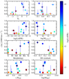 |
Fig. 9 Peculiar velocity correction, c|Δz|, for SNe Ia that belong to clusters, as a function of supernova parameters (X1, C; triangles), host properties (local specific SFR (yr−1 kpc−2), stellar mass (M⊙), morphological type, RS residuals [ |

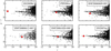 |
Fig. 10 Color-magnitude diagram (g − r vs. r) plotted for the clusters from Table 1 for the six clusters for which SDSS galaxy redshifts and colors are available (Eisenstein et al. 2011; Dawson et al. 2013; Smee et al. 2013; SDSS Collaboration 2017). Red points show the positions of supernova hosts, most of which are located near the red sequence. |
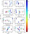 |
Fig. 11 Absolute change in HRs due to peculiar velocity correction for SNe Ia that belong to clusters as a function of supernova parameters (X1, C; triangles), host properties (local specific SFR (yr−1kpc−2), stellarmass (M⊙), morphological type, RS residuals [ |
6 Conclusions
Unknown peculiar velocities are an additional source of uncertainty on the Hubble diagram. Usually, they are taken into account by assuming 150–300 km s−1 as an additional statistical uncertainty in the calculations or by applying corrections based on linear flow maps. However, the velocity dispersion for galaxies inside galaxy clusters can be much higher than these methods account for. In this paper we developed a method for assigning SNe Ia to clusters, we studied how the peculiar velocities of SNe Ia in galaxy clusters affect the redshift measurement and propagate through to the distance estimation. We tested the match of 145 SNe Ia observed by SNFACTORY with known clusters of galaxies and used the cluster redshift to measure the redshifts of the SNe Ia instead of the host galaxy redshift. Among the full sample of SNe Ia, 11 were found to be in clusters of galaxies.
The technique we developed improved the redshift measurements for low and intermediate redshifts (z < 0.1) and decreased the spread on the Hubble diagram. When peculiar velocities are taken into account for the SNe in clusters, the wRMS = 0.130 ± 0.038 mag is smaller than the wRMS = 0.137 ± 0.036 mag found when no correction is applied. The correction is statistically significant with a value of 3.58σ; however, when we exclude SN2006X the significance of the correction decreases to 1.34σ.
We also found that the Hubble diagram dispersion of the 11 SNe Ia that belong to clusters is smaller than for SNe in the field, but with a P-value of 3.8 × 10⁻¹, which is not statistically significant. Among 11 SNe found in clusters, the SNe Ia hosted by blue spiral galaxies, which have high local sSFR, smaller Mstellar, r∕R200 ≃ 0.7, show higher peculiar velocity corrections (see Fig. 9).
Since the majority of galaxies in the Universe are not found in galaxy clusters, but in filamentary structures such as the Great Wall (Geller & Huchra 1989), SNe Ia in galaxy clusters are rare in untargeted searches such as SNFACTORY. Next decade surveys such as the Zwicky Transient Facility (ZTF) or the Large Synoptic Survey Telescope (LSST; Bellm 2014; LSST Science Collaboration 2009) will observe thousands of SNe Ia and therefore have much larger samples of SNe Ia in clusters. These can be used to study dependencies between SNe Ia and host clusters with greater certainty. LSST will be much deeper than SNFACTORY or ZTF, so the method of cluster selection based only on the presence of X-rays will not be viable until much deeper all-sky X-ray surveys are performed. Even though the impact of peculiar velocities decreases with distance and becomes negligible at high redshifts, SN Ia rates in clusters (Sharon et al. 2010; Barbary et al. 2012) and the difference in SN light curve parameters inside and outside the clusters could be fruitful avenues of investigation for future cosmological analyses.
Acknowledgements
We thank the technical staff of the University of Hawaii 2.2 m telescope and Dan Birchall for observing assistance. We recognize the significant cultural role of Mauna Kea within the indigenous Hawaiian community, and we appreciate the opportunity to conduct observations from this revered site. This work was supported in part by the Director, Office of Science, Office of High Energy Physics of the U.S. Department of Energy under Contract No. DE-AC025CH11231. Support in France was provided by CNRS/IN2P3, CNRS/INSU, and PNC; LPNHE acknowledges support from LABEX ILP, supported by French state funds managed by the ANR within the Investissements d’Avenir programme under reference ANR-11-IDEX-0004-02. NC is grateful to the LABEX Lyon Institute of Origins (ANR-10-LABX-0066) of the University de Lyon for its financial support within the program “Investissements d’Avenir” (ANR-11-IDEX-0007) of the French government operated by the National Research Agency (ANR). Support in Germany was provided by DFG through TRR33 “The Dark Universe” and by DLR through grants FKZ 50OR1503 and FKZ 50OR1602. In China support was provided by Tsinghua University 985 grant and NSFC grant No 11173017. Some results were obtained using resources and support from the National Energy Research Scientific Computing Center, supported by the Director, Office of Science, Office of Advanced Scientific Computing Research of the U.S. Department of Energy under Contract No. DE-AC02-05CH11231. We thank the Gordon & Betty Moore Foundation for their continuing support. Additional support was provided by NASA under the Astrophysics Data Analysis Program grant 15-ADAP15-0256 (PI: Aldering). We also thank the High Performance Research and Education Network (HPWREN), supported by National Science Foundation Grant Nos. 0087344 & 0426879. This project has received funding from the European Research Council (ERC) under the European Union’s Horizon 2020 research and innovation programme (grant agreement No 759194 – USNAC). P.F.L. acknowledges support from the National Science Foundation grant PHY-1404070. M.V.P. acknowledges support from Russian Science Foundation grant 14-12-00146 for the selection of SNe exploded in galaxy clusters. This research has made use of the NASA/IPAC Extragalactic Database (NED), which is operated by the Jet Propulsion Laboratory, California Institute of Technology, under contract with the National Aeronautics and Space Administration. Funding for the Sloan Digital Sky Survey IV has been provided by the Alfred P. Sloan Foundation, the U.S. Department of Energy Office of Science, and the Participating Institutions. SDSS-IV acknowledges support and resources from the Center for High-Performance Computing at the University of Utah. The SDSS web site is www.sdss.org. SDSS-IV is managed by the Astrophysical Research Consortium for the Participating Institutions of the SDSS Collaboration including the Brazilian Participation Group, the Carnegie Institution for Science, Carnegie Mellon University, the Chilean Participation Group, the French Participation Group, Harvard-Smithsonian Center for Astrophysics, Instituto de Astrofísica de Canarias, The Johns Hopkins University, Kavli Institute for the Physics and Mathematics of the Universe (IPMU)/University of Tokyo, Lawrence Berkeley National Laboratory, Leibniz Institut für Astrophysik Potsdam (AIP), Max-Planck-Institut für Astronomie (MPIA Heidelberg), Max-Planck-Institut für Astrophysik (MPA Garching), Max-Planck-Institut für Extraterrestrische Physik (MPE), National Astronomical Observatories of China, New MexicoState University, New York University, University of Notre Dame, Observatário Nacional/MCTI, The Ohio State University, Pennsylvania State University, Shanghai Astronomical Observatory, United Kingdom Participation Group, Universidad Nacional Autónoma de México, University of Arizona, University of Colorado Boulder, University of Oxford, University of Portsmouth, University of Utah, University of Virginia, University of Washington, University of Wisconsin, Vanderbilt University, and Yale University. This research has made use of the SIMBAD database, operated at CDS, Strasbourg, France. We acknowledge the usage of the HYPERLEDA database (http://leda.univ-lyon1.fr). We have made use of the ROSAT Data Archive of the Max-Planck-Institut für extraterrestrische Physik (MPE) at Garching, Germany.
References
- Abell, G. O. 1958, ApJS, 3, 211 [NASA ADS] [CrossRef] [Google Scholar]
- Abell, G. O., Corwin, Jr., H. G., & Olowin, R. P. 1989, ApJS, 70, 1 [NASA ADS] [CrossRef] [EDP Sciences] [Google Scholar]
- Aldering, G., Adam, G., Antilogus, P., et al. 2002, SPIE Conf. Ser., 4836, 61 [Google Scholar]
- Aldering, G., Antilogus, P., Bailey, S., et al. 2006, ApJ, 650, 510 [NASA ADS] [CrossRef] [Google Scholar]
- Amanullah, R., Lidman, C., Rubin, D., et al. 2010, ApJ, 716, 712 [NASA ADS] [CrossRef] [Google Scholar]
- Arnaud, M., Pratt, G. W., Piffaretti, R., et al. 2010, A&A, 517, A92 [NASA ADS] [CrossRef] [EDP Sciences] [Google Scholar]
- Astier, P., Guy, J., Regnault, N., et al. 2006, A&A, 447, 31 [NASA ADS] [CrossRef] [EDP Sciences] [Google Scholar]
- Bahcall, N. A., & Oh, S. P. 1996, ApJ, 462, L49 [NASA ADS] [CrossRef] [EDP Sciences] [Google Scholar]
- Bailey, S., Aldering, G., Antilogus, P., et al. 2009, A&A, 500, L17 [NASA ADS] [CrossRef] [EDP Sciences] [Google Scholar]
- Barbary, K., Aldering, G., Amanullah, R., et al. 2012, ApJ, 745, 32 [NASA ADS] [CrossRef] [Google Scholar]
- Beers, T. C., Flynn, K., & Gebhardt, K. 1990, AJ, 100, 32 [NASA ADS] [CrossRef] [Google Scholar]
- Bellm, E. 2014, in The Third Hot-wiring the Transient, eds. P. R. Wozniak, M. J. Graham, A. A. Mahabal, & R. Seaman, 27 [Google Scholar]
- Betoule, M., Kessler, R., Guy, J., et al. 2014, A&A, 568, 32 [Google Scholar]
- Blakeslee, J. P., Davis, M., Tonry, J. L., Dressler, A., & Ajhar, E. A. 1999, ApJ, 527, L73 [NASA ADS] [CrossRef] [EDP Sciences] [Google Scholar]
- Blondin, S., Mandel, K. S., & Kirshner, R. P. 2011, A&A, 526, A81 [NASA ADS] [CrossRef] [EDP Sciences] [Google Scholar]
- Blondin, S., Matheson, T., Kirshner, R. P., et al. 2012, AJ, 143, 126 [NASA ADS] [CrossRef] [Google Scholar]
- Boldt, E., McDonald, F. B., Riegler, G., & Serlemitsos, P. 1966, Phys. Rev. Lett., 17, 447 [NASA ADS] [CrossRef] [Google Scholar]
- Bongard, S., Soulez, F., Thiébaut, É., & Pecontal, É. 2011, MNRAS, 418, 258 [NASA ADS] [CrossRef] [Google Scholar]
- Brown, M. J. I., Moustakas, J., Smith, J.-D. T., et al. 2014, ApJS, 212, 18 [Google Scholar]
- Buton, C., Copin, Y., Aldering, G., et al. 2013, A&A, 549, A8 [NASA ADS] [CrossRef] [EDP Sciences] [Google Scholar]
- Carlberg, R. G., Yee, H. K. C., & Ellingson, E. 1997, ApJ, 478, 462 [NASA ADS] [CrossRef] [EDP Sciences] [Google Scholar]
- Childress, M., Aldering, G., Antilogus, P., et al. 2013, ApJ, 770, 107 [NASA ADS] [CrossRef] [Google Scholar]
- Chotard, N., Gangler, E., Aldering, G., et al. 2011, A&A, 529, L4 [NASA ADS] [CrossRef] [EDP Sciences] [Google Scholar]
- Clowe, D., Bradač, M., Gonzalez, A. H., et al. 2006, ApJ, 648, L109 [NASA ADS] [CrossRef] [Google Scholar]
- Colless, M., & Dunn, A. M. 1996, ApJ, 458, 435 [NASA ADS] [CrossRef] [Google Scholar]
- Conley, A., Guy, J., Sullivan, M., et al. 2011, ApJS, 192, 1 [NASA ADS] [CrossRef] [EDP Sciences] [Google Scholar]
- Cooray, A., & Caldwell, R. R. 2006, Phys. Rev. D, 73, 103002 [NASA ADS] [CrossRef] [Google Scholar]
- Cruddace, R., Voges, W., Böhringer, H., et al. 2002, ApJS, 140, 239 [NASA ADS] [CrossRef] [Google Scholar]
- Dale, D. A., Giovanelli, R., Haynes, M. P., Campusano, L. E., & Hardy, E. 1999, ApJ, 118, 1489 [NASA ADS] [CrossRef] [Google Scholar]
- Davis, T. M., Hui, L., Frieman, J. A., et al. 2011, ApJ, 741, 67 [NASA ADS] [CrossRef] [Google Scholar]
- Dawson, K. S., Schlegel, D. J., Ahn, C. P., et al. 2013, AJ, 145, 10 [Google Scholar]
- Dhawan, S., Jha, S. W., & Leibundgut, B. 2018, A&A, 609, A72 [NASA ADS] [CrossRef] [EDP Sciences] [Google Scholar]
- Dilday, B., Bassett, B., Becker, A., et al. 2010, ApJ, 715, 1021 [NASA ADS] [CrossRef] [Google Scholar]
- Durret, F., Forman, W., Gerbal, D., Jones, C., & Vikhlinin, A. 1998, A&A, 335, 41 [NASA ADS] [Google Scholar]
- Eisenstein, D. J., Weinberg, D. H., Agol, E., et al. 2011, AJ, 142, 72 [Google Scholar]
- Fakhouri, H. K., Boone, K., Aldering, G., et al. 2015, ApJ, 815, 58 [NASA ADS] [CrossRef] [Google Scholar]
- Feindt, U., Kerschhaggl, M., Kowalski, M., et al. 2013, A&A, 560, A90 [NASA ADS] [CrossRef] [EDP Sciences] [Google Scholar]
- Geller, M. J., & Huchra, J. P. 1989, Science, 246, 897 [NASA ADS] [CrossRef] [PubMed] [Google Scholar]
- Gladders, M. D., & Yee, H. K. C. 2000, AJ, 120, 2148 [NASA ADS] [CrossRef] [Google Scholar]
- Gunn, J. E., Hoessel, J. G., & Oke, J. B. 1986, ApJ, 306, 30 [Google Scholar]
- Guy, J., Astier, P., Nobili, S., Regnault, N., & Pain, R. 2005, A&A, 443, 781 [NASA ADS] [CrossRef] [EDP Sciences] [Google Scholar]
- Guy, J., Astier, P., Baumont, S., et al. 2007, A&A, 466, 11 [NASA ADS] [CrossRef] [EDP Sciences] [Google Scholar]
- Guy, J., Sullivan, M., Conley, A., et al. 2010, A&A, 523, A7 [NASA ADS] [CrossRef] [EDP Sciences] [Google Scholar]
- Habibi, F., Baghram, S., & Tavasoli, S. 2018, Int. J. Mod. Phys. D, 27, 1850019 [NASA ADS] [CrossRef] [Google Scholar]
- Hamuy, M., Phillips, M. M., Maza, J., et al. 1995, AJ, 109, 1 [NASA ADS] [CrossRef] [Google Scholar]
- Hamuy, M., Phillips, M. M., Suntzeff, N. B., et al. 1996a, AJ, 112, 2391 [NASA ADS] [CrossRef] [Google Scholar]
- Hamuy, M., Phillips, M. M., Suntzeff, N. B., et al. 1996b, AJ, 112, 2398 [NASA ADS] [CrossRef] [Google Scholar]
- Hamuy, M., Trager, S. C., Pinto, P. A., et al. 2000, AJ, 120, 1479 [NASA ADS] [CrossRef] [Google Scholar]
- Henne, V., Pruzhinskaya, M. V., Rosnet, P., et al. 2017, New Ast., 51, 43 [NASA ADS] [CrossRef] [Google Scholar]
- Hill, R., Shariff, H., Trotta, R., et al. 2016, MNRAS, submitted [arXiv:1612.04417] [Google Scholar]
- Hudson, M. J., Lucey, J. R., Smith, R. J., Schlegel, D. J., & Davies, R. L. 2001, MNRAS, 327, 265 [NASA ADS] [CrossRef] [Google Scholar]
- Hudson, M. J., Smith, R. J., Lucey, J. R., & Branchini, E. 2004, MNRAS, 352, 61 [Google Scholar]
- Hui, L., & Greene, P. B. 2006, Phys. Rev. D, 73, 12 [NASA ADS] [CrossRef] [Google Scholar]
- Jha, S., Riess, A. G., & Kirshner, R. P. 2007, ApJ, 659, 122 [NASA ADS] [CrossRef] [Google Scholar]
- Johansson, J., Thomas, D., Pforr, J., et al. 2013, MNRAS, 435, 1680 [NASA ADS] [CrossRef] [Google Scholar]
- Karachentsev, I. D., Tully, R. B., Wu, P.-F., Shaya, E. J., & Dolphin, A. E. 2014, ApJ, 782, 4 [NASA ADS] [CrossRef] [Google Scholar]
- Kelly, P. L., Hicken, M., Burke, D. L., Mandel, K. S., & Kirshner, R. P. 2010, ApJ, 715, 743 [NASA ADS] [CrossRef] [Google Scholar]
- Kepner, J., Fan, X., Bahcall, N., et al. 1999, ApJ, 517, 78 [NASA ADS] [CrossRef] [Google Scholar]
- Kim, A. G., Thomas, R. C., Aldering, G., et al. 2013, ApJ, 766, 84 [NASA ADS] [CrossRef] [Google Scholar]
- Kim, S., Rey, S.-C., Jerjen, H., et al. 2014, ApJS, 215, 22 [Google Scholar]
- Lantz, B., Aldering, G., Antilogus, P., et al. 2004, SPIE Conf. Ser., 5249, 146 [Google Scholar]
- Law, N. M., Kulkarni, S. R., Dekany, R. G., et al. 2009, PASP, 121, 1395 [NASA ADS] [CrossRef] [Google Scholar]
- Léget, P.-F. 2016, PhD Thesis, Université Blaise Pascal, France [Google Scholar]
- Li, W. 2005, IAU Circ., 8611 [Google Scholar]
- LSST Science Collaboration (Abell, P. A., et al.) 2009, ArXiv e-prints [arXiv: 0912.0201] [Google Scholar]
- Makarov, D., Prugniel, P., Terekhova, N., Courtois, H., & Vauglin, I. 2014, A&A, 570, A13 [CrossRef] [EDP Sciences] [Google Scholar]
- Masters, K. L., Springob, C. M., Haynes, M. P., & Giovanelli, R. 2006, ApJ, 653, 861 [NASA ADS] [CrossRef] [Google Scholar]
- Mickaelian, A. M., Hovhannisyan, L. R., Engels, D., Hagen, H.-J., & Voges, W. 2006, A&A, 449, 425 [NASA ADS] [CrossRef] [EDP Sciences] [Google Scholar]
- Mulchaey, J. S. 2000, ARA&A, 38, 289 [NASA ADS] [CrossRef] [Google Scholar]
- Nakano, S., Itagaki, K., Li, W., Cenko, S. B., & Filippenko, A. V. 2009, Central Bureau Electronic Telegrams, 1872 [Google Scholar]
- Neill, J. D. Hudson, M. J., & Conley, A. 2007, ApJ, 661, L123 [NASA ADS] [CrossRef] [Google Scholar]
- Neill, J. D., Sullivan, M., Howell, D. A., et al. 2009, ApJ, 707, 1449 [NASA ADS] [CrossRef] [Google Scholar]
- Nugent, P., Sullivan, M., & Howell, D. A. 2009, ATel, 2255, 1 [NASA ADS] [Google Scholar]
- Patat, F., Chandra, P., Chevalier, R., et al. 2007, Science, 317, 924 [NASA ADS] [CrossRef] [EDP Sciences] [PubMed] [Google Scholar]
- Patat, F., Baade, D., Höflich, P., et al. 2009, A&A, 508, 229 [NASA ADS] [CrossRef] [EDP Sciences] [Google Scholar]
- Pereira, R., Thomas, R. C., Aldering, G., et al. 2013, A&A, 554, A27 [NASA ADS] [CrossRef] [EDP Sciences] [Google Scholar]
- Perlmutter, S., Gabi, S., Goldhaber, G., et al. 1997, ApJ, 483, 565 [NASA ADS] [CrossRef] [Google Scholar]
- Perlmutter, S., Aldering, G., della Valle, M., et al. 1998, Nature, 391, 51 [CrossRef] [Google Scholar]
- Perlmutter, S., Aldering, G., Goldhaber, G., et al. 1999, ApJ, 517, 565 [NASA ADS] [CrossRef] [Google Scholar]
- Phillips, M. M. 1993, ApJ, 413, L105 [NASA ADS] [CrossRef] [Google Scholar]
- Phillips, M. M., Lira, P., Suntzeff, N. B., et al. 1999, AJ, 118, 1766 [NASA ADS] [CrossRef] [Google Scholar]
- Piffaretti, R., Arnaud, M., Pratt, G. W., Pointecouteau, E., & Melin, J.-B. 2011, A&A, 534, A109 [NASA ADS] [CrossRef] [EDP Sciences] [Google Scholar]
- Planck Collaboration XXIV. 2016, A&A, 594, A24 [NASA ADS] [CrossRef] [EDP Sciences] [Google Scholar]
- Planck Collaboration XXVII. 2016, A&A, 594, A27 [NASA ADS] [CrossRef] [EDP Sciences] [Google Scholar]
- Pskovskii, I. P. 1977, Sov. Astron., 21, 675 [NASA ADS] [Google Scholar]
- Pskovskii, Y. P. 1984, Sov. Astron., 28, 658 [NASA ADS] [Google Scholar]
- Quimby, R., Yuan, F., Akerloff, C., et al. 2007, Central Bureau Electronic Telegrams, 1106 [Google Scholar]
- Rabinowitz, D., Baltay, C., Emmet, W., et al. 2003, BAAS, 35, 1262 [NASA ADS] [Google Scholar]
- Radburn-Smith, D. J., Lucey, J. R., & Hudson, M. J. 2004, MNRAS, 355, 1378 [Google Scholar]
- Reiprich, T. H., & Böhringer, H. 2002, ApJ, 567, 716 [NASA ADS] [CrossRef] [Google Scholar]
- Riess, A., Press, W., & Kirshner, R. 1996, AJ, 473, 88 [Google Scholar]
- Riess, A. G., Davis, M., Baker, J., & Kirshner, R. P. 1997, ApJ, 488, L1 [NASA ADS] [CrossRef] [Google Scholar]
- Riess, A. G., Filippenko, A. V., Challis, P., et al. 1998, AJ, 116, 1009 [NASA ADS] [CrossRef] [Google Scholar]
- Riess, A. G., Kirshner, R. P., Schmidt, B. P., et al. 1999, AJ, 117, 707 [Google Scholar]
- Rigault, M., Copin, Y., Aldering, G., et al. 2013, A&A, 560, A66 [NASA ADS] [CrossRef] [EDP Sciences] [Google Scholar]
- Rigault, M., Brinnel, V., Aldering, G., et al. 2018, A&A, submitted [arXiv:1806.03849] [Google Scholar]
- Rines, K., & Diaferio, A. 2006, AJ, 132, 1275 [NASA ADS] [CrossRef] [Google Scholar]
- Ruel, J., Bazin, G., Bayliss, M., et al. 2014, ApJ, 792, 45 [Google Scholar]
- Rust, B. W. 1974, PhD Thesis, Oak Ridge National Lab., TN, USA [Google Scholar]
- Sarazin, C. L. 1988, X-ray Emission from Clusters of Galaxies (London: Cambridge University Press) [Google Scholar]
- Sasdelli, M., Ishida, E. E. O., Hillebrandt, W., et al. 2016, MNRAS, 460, 373 [NASA ADS] [CrossRef] [Google Scholar]
- Scalzo, R. A., Aldering, G., Antilogus, P., et al. 2010, ApJ, 713, 1073 [NASA ADS] [CrossRef] [Google Scholar]
- Schmidt, B. P., Suntzeff, N. B., Phillips, M. M., et al. 1998, ApJ, 507, 46 [NASA ADS] [CrossRef] [Google Scholar]
- Scolnic, D. M., Jones, D. O., Rest, A., et al. 2017, ApJ, 859, 101 [Google Scholar]
- SDSS Collaboration (Albareti, F. D., et al.) 2017, ApJS, 233, 25 [NASA ADS] [CrossRef] [Google Scholar]
- Sharon, K., Gal-Yam, A., Maoz, D., et al. 2010, ApJ, 718, 876 [NASA ADS] [CrossRef] [Google Scholar]
- Smee, S. A., Gunn, J. E., Uomoto, A., et al. 2013, AJ, 146, 32 [Google Scholar]
- Smith, R. J., Hudson, M. J., Nelan, J. E., et al. 2004, AJ, 128, 1558 [NASA ADS] [CrossRef] [Google Scholar]
- Smith, M., Nichol, R. C., Dilday, B., et al. 2012, ApJ, 755, 61 [NASA ADS] [CrossRef] [Google Scholar]
- Sternberg, A., Gal-Yam, A., Simon, J. D., et al. 2011, Science, 333, 856 [NASA ADS] [CrossRef] [Google Scholar]
- Sullivan, M., Ellis, R. S., Aldering, G., et al. 2003, MNRAS, 340, 1057 [NASA ADS] [CrossRef] [Google Scholar]
- Sullivan, M., Le Borgne, D., Pritchet, C. J., et al. 2006, ApJ, 648, 868 [NASA ADS] [CrossRef] [Google Scholar]
- Sullivan, M., Conley, A., Howell, D. A., et al. 2010, MNRAS, 406, 782 [NASA ADS] [Google Scholar]
- Suzuki, S., & Migliardi, M. 2006, IAU Circ., 8667 [Google Scholar]
- Suzuki, N., Rubin, D., Lidman, C., et al. 2012, ApJ, 746, 85 [NASA ADS] [CrossRef] [Google Scholar]
- Tonry, J. L., & Davis, M. 1981, ApJ, 246, 680 [NASA ADS] [CrossRef] [Google Scholar]
- Tully, R. B., & Fisher, J. R. 1977, A&A, 54, 661 [NASA ADS] [Google Scholar]
- Tully, R. B., & Shaya, E. J. 1984, ApJ, 281, 31 [NASA ADS] [CrossRef] [Google Scholar]
- Ulrich, M.-H. 1976, ApJ, 206, 364 [NASA ADS] [CrossRef] [Google Scholar]
- Vikhlinin, A., McNamara, B. R., Forman, W., et al. 1998, ApJ, 502, 558 [NASA ADS] [CrossRef] [Google Scholar]
- Wang, L., Goldhaber, G., Aldering, G., & Perlmutter, S. 2003, ApJ, 590, 944 [NASA ADS] [CrossRef] [Google Scholar]
- Wang, X., Filippenko, A. V., Ganeshalingam, M., et al. 2009, ApJ, 699, L139 [NASA ADS] [CrossRef] [Google Scholar]
- Wegner, G., Haynes, M. P., & Giovanelli, R. 1993, AJ, 105, 1251 [NASA ADS] [CrossRef] [Google Scholar]
- Wenger, M., Ochsenbein, F., Egret, D., et al. 2000, A&AS, 143, 9 [NASA ADS] [CrossRef] [EDP Sciences] [Google Scholar]
- Willick, J. A.,& Strauss, M. A. 1998, ApJ, 507, 64 [NASA ADS] [CrossRef] [Google Scholar]
- Wood-Vasey, W. M., Miknaitis, G., Stubbs, C. W., et al. 2007, ApJ, 666, 694 [NASA ADS] [CrossRef] [Google Scholar]
- Wu, H.-Y., Hahn, O., Wechsler, R. H., Mao, Y.-Y., & Behroozi, P. S. 2013, ApJ, 763, 70 [NASA ADS] [CrossRef] [Google Scholar]
- Xavier, H. S., Gupta, R. R., Sako, M., et al. 2013, MNRAS, 434, 1443 [NASA ADS] [CrossRef] [Google Scholar]
- Zwicky, F., Herzog, E., Wild, P., Karpowicz, M., & Kowal, C. T. 1961, Catalogue of Galaxies and of Clusters of Galaxies I (Pasadena: California Institute of Technology) [Google Scholar]
Hereafter, we refer to this procedure as peculiar velocity correction.
Taking into account all the SNe Ia does not affect the Hubble diagram fitting because the number of SNe Ia inside galaxy clusters is small.
All Tables
All Figures
|
Fig. 1 Hubble diagram demonstrating how large peculiar velocity can affect the measurements of the expansion history of the Universe. The inset plot is a typical velocity distribution of galaxies inside a cluster. |
| In the text | |
|
Fig. 2 Redshift uncertainties (in magnitude units) due to different levels of peculiar velocities as a function of the cosmological redshift. The solid black line corresponds to the Coma cluster velocity dispersion; the dashed and dash-dotted lines correspond to 300 and 150 km s−1, respectively. The red line shows the intrinsic dispersion of SNe Ia on the Hubble diagram found for the JLA sample (Betoule et al. 2014). |
| In the text | |
|
Fig. 3 Luminosities of [0.1–2.4 keV] within R500 of MCXC clusters (Piffaretti et al. 2011) as a function of redshift, up to z = 0.1. The colorbarshows the corresponding cluster velocity dispersion σV calculated from Eq. (7). Black plus signs indicate clusters from the current analysis. The black curve corresponds to the intrinsic dispersion of SNe Ia on the Hubble diagram found for the JLA sample (Betoule et al. 2014) projected onto cluster luminosities by combining the luminosity–mass and mass–velocity dispersion relations. |
| In the text | |
|
Fig. 4 Workflow for redshift calculation and other inputs for matching of SNe to galaxy clusters. In this scheme, Ngal corresponds to the number of galaxies used to compute the redshift and Npaper corresponds to the number of galaxies used to estimate the redshift in the literature. |
| In the text | |
|
Fig. 5 Speed normalized by velocity dispersion within the ensemble cluster vs. the distance between galaxies and ensemble cluster normalized by R200. The small points indicate galaxies with spectroscopy from SDSS. The big points represent the positions of host galaxies of our SNe Ia. The color bar shows the corresponding g− r color; the points filled with gray do not have color measurements. The solid lines show the cuts we applied to associate SNe Ia withclusters, and the dashed lines represent the prolongation of those cuts. |
| In the text | |
|
Fig. 6 Hubble diagram residuals. For cluster members red circles (blue squares) and histograms correspond to residuals for SNe Ia in galaxy clusters before (after) correction for peculiar velocities of the hosts inside their clusters. The black histogram corresponds to all SNe Ia after correction. SN2006X is presented in the inset plot separately from the others owing to its very large offset. |
| In the text | |
|
Fig. 7 Velocity pull distribution (in blue) in comparison with a Gaussian distribution with the observed standard distribution of the velocity pull. This is compatible with the expected standard deviation of unity. |
| In the text | |
|
Fig. 8 Distribution of the difference in absolute HR after (HRa) and before (HRb) peculiar velocity correction (in blue). The black line represents the expected distribution of the difference in HR, and the red curve is the expected change convolved with error distribution. The results are compatible with the observed distribution given the Poisson uncertainties of each histogram bin. |
| In the text | |
|
Fig. 9 Peculiar velocity correction, c|Δz|, for SNe Ia that belong to clusters, as a function of supernova parameters (X1, C; triangles), host properties (local specific SFR (yr−1 kpc−2), stellar mass (M⊙), morphological type, RS residuals [ |
| In the text | |
|
Fig. 10 Color-magnitude diagram (g − r vs. r) plotted for the clusters from Table 1 for the six clusters for which SDSS galaxy redshifts and colors are available (Eisenstein et al. 2011; Dawson et al. 2013; Smee et al. 2013; SDSS Collaboration 2017). Red points show the positions of supernova hosts, most of which are located near the red sequence. |
| In the text | |
|
Fig. 11 Absolute change in HRs due to peculiar velocity correction for SNe Ia that belong to clusters as a function of supernova parameters (X1, C; triangles), host properties (local specific SFR (yr−1kpc−2), stellarmass (M⊙), morphological type, RS residuals [ |
| In the text | |
Current usage metrics show cumulative count of Article Views (full-text article views including HTML views, PDF and ePub downloads, according to the available data) and Abstracts Views on Vision4Press platform.
Data correspond to usage on the plateform after 2015. The current usage metrics is available 48-96 hours after online publication and is updated daily on week days.
Initial download of the metrics may take a while.