| Issue |
A&A
Volume 615, July 2018
|
|
|---|---|---|
| Article Number | A76 | |
| Number of page(s) | 28 | |
| Section | Stellar atmospheres | |
| DOI | https://doi.org/10.1051/0004-6361/201731533 | |
| Published online | 17 July 2018 | |
Spectroscopic Parameters and atmosphEric ChemIstriEs of Stars (SPECIES)
I. Code description and dwarf stars catalogue★
1
Departamento de Astronomía, Universidad de Chile,
Casilla 36-D,
Camino el Observatorio 1515,
Las Condes,
Santiago,
Chile
e-mail: This email address is being protected from spambots. You need JavaScript enabled to view it.
2
Centro de Astrofísica y Tecnologías Afines (CATA),
Casilla 36-D,
Santiago,
Chile
Received:
7
August
2017
Accepted:
14
March
2018
Abstract
Context. The detection and subsequent characterisation of exoplanets are intimately linked to the characteristics of their host star. Therefore, it is necessary to study the star in detail in order to understand the formation history and characteristics of their companion(s).
Aims. Our aims are to develop a community tool that allows the automated calculation of stellar parameters for a large number of stars, using high resolution echelle spectra and minimal photometric magnitudes, and introduce the first catalogue of these measurements in this work.
Methods. We measured the equivalent widths of several iron lines and used them to solve the radiative transfer equation assuming local thermodynamic equilibrium in order to obtain the atmospheric parameters (Teff, [Fe/H], logg, and ξt). We then used these values to derive the abundance of 11 chemical elements in the stellar photosphere (Na, Mg, Al, Si, Ca, Ti, Cr, Mn, Ni, Cu, and Zn). Rotation and macroturbulent velocity were obtained using temperature calibrators and synthetic line profiles to match the observed spectra of five absorption lines. Finally, by interpolating in a grid of MIST isochrones, we were able to derive the mass, radius, and age for each star using a Bayesian approach.
Results. SPECIES obtains bulk parameters that are in good agreement with measured values from different existing catalogues, including when different methods are used to derive them. We find discrepancies in the chemical abundances for some elements with respect to other works, which could be produced by differences in Teff, or in the line list or the atomic line data used to derive them. We also obtained analytic relations to describe the correlations between different parameters, and we implemented new methods to better handle these correlations, which provides a better description of the uncertainties associated with the measurements.
Key words: techniques: spectroscopic / stars: abundances / fundamental parameters
The full Table D.1 is only available at the CDS via anonymous ftp to cdsarc.u-strasbg.fr (130.79.128.5) or via http://cdsarc.u-strasbg.fr/viz-bin/qcat?J/A+A/615/A76
© ESO 2018
1 Introduction
The characterisation of exoplanetary systems has become a booming field of study in astronomy over the last 20 yr, thanks to the large amount of detections provided by different surveys from different telescopes and instruments (CORALIE, Keck, HARPS, AAT, WASP, Kepler, K2, etc.). Unfortunately, the low surface brightness and size of planets compared to their host star, makes them extremely difficult to study directly, therefore it is necessary to study the behaviour and physical parameters of the host stars in order to better characterise their planetary companions. These parameters include the temperature, metallicity, surface gravity, mass, and age, which in turn gives us an estimate of their evolutionary stages.
Calculation of the stellar bulk parameters, like temperature, metallicity and mass, is vital to derive the physical characteristics of the companions. The minimum mass of the planetary candidates can be obtained by the amplitude of the star’s radial velocity, which in turn depends on the mass of the host star, among other parameters. Planetary sizes can be inferred by studying the decrease in brightness of the host star when the planet transits, which in turn depends on the diameter of the star. By knowing the mass and physical size of a planetary companion, it is possible to understand its chemical composition, since the planet bulk density can be calculated. This information, combined with the knowledge of the stellar effective temperature (Teff) and the orbital distance of the planet, allows a probability to be placed on the likelihood that the planet has liquid water in its atmosphere, and/or on its surface. Knowledge of the stellar parameters is also needed in order to study the formation of planetary companions (Fischer & Valenti 2005; Buchhave et al. 2012; Jenkins et al. 2013), how the system has evolved to its current stage (Ida & Lin 2004, 2005; Mordasini et al. 2012), and how the subsequence evolution of the host star will affect the planetary system (Villaver & Livio 2009; Kunitomo et al. 2011; Jones et al. 2016).
The derivation of stellar parameters is not something new in astrophysics. Many works have dealt with this task, employing different methods in order to obtain them. The most common methods in the literature are using equivalent width (EW) measurements (e.g. Edvardsson et al. 1993; Feltzing & Gustafsson 1998; Santos et al. 2004; Bond et al. 2006; Neves et al. 2009), and the spectral synthesis approach (e.g. Valenti & Fischer 2005; Jenkins et al. 2008; Pavlenko et al. 2012). The results produced by different methods show significant systematic differences (Torres et al. 2012; Ivanyuk et al. 2017), which then can affect the physical characteristics of any detected companions. When the values for the stellar parameters are retrieved from different sources, it can lead to problems when studying populations of stars. This is often necessary because not all catalogues of stellar parameters have all the quantities needed, or uncertainties in the values are not listed, making it difficult to implement them in other studies (e.g. see the analysis presented in Jenkins et al. 2017). Another barrier that one finds when studying stellar parameters is that most works are limited to the stars included in their resulting catalogues, making it difficult to compute parameters for new stars in a homogeneous way. All of these issues were behind the development of the SPECIES code, an open source method that can compute stellar parameters for large numbers of stars in a homogeneous and self-consistent fashion, and crucially, that is publicly available to the scientific community1.
The SPECIES code is written mostly in the python programming language, making use of some previously developed software (e.g. MOOG, Sneden 1973; ARES, Sousa et al. 2007) that allows automatic calculations of specific jobs to be performed, with the goal of increasing the speed of the process whilst subsequently decreasing the user input for the derivation of the stellar parameters. The code is automated in the computation of all the parameters, and the only input from the user is a high resolution spectrum of the desired star. It can be used with only one star at a time, or several stars at once running in parallel. This makes it possible to derive the parameters for large samples of stars, a necessity in this new era of exoplanet surveys (e.g. NGTS, ESPRESSO, TESS, etc.), with the number of planetary candidates increasing each month.
The paper structure is as follows. Section 2 explains the inputs needed to run the code, and its final output. Here we also list the atomic lines used (Sect. 2.1), we explain in detail the derivation of the atmospheric parameters and their corresponding uncertainties (Sects. 2.4 and 2.5, respectively), the stellar mass, radii and age (Sect. 2.6), the chemical abundances of different elements (Sect. 2.7), and the computation of the macroturbulence and rotational velocity (Sect. 2.8). Section 3 shows the results obtained using our code for a sample of 522 stars, how those values compare to others in the literature (Sect. 3.2), and the difference obtained when using spectra from different instruments (Sect. 3.4). In Sect. 3.3 we show thecorrelations between the parameters that we find in our results. Finally, in Sect. 4 we give a summary of the characteristics and use of SPECIES and how we plan to continue to develop the code in the future.
2 Stellar parameter computation
SPECIES isan automatic code that computes stellar atmospheric parameters in a self-consistent and homogeneous way: effective temperature, surface gravity, metallicity with respect to the Sun, and microturbulent velocity (Teff, log g, [Fe/H], and ξt respectively). Our code also derives chemical abundances for 11 additional atomic elements, rotational and macroturbulence velocity, along with stellar mass, age, radius, and photometric log g. The uncertainties of each parameter are also computed in a consistent way, dealing with parameter correlations and propagation of uncertainties, all of which will be discussed in the following sections.
The inputs needed for our code to perform all computations are:
A high resolution (R > 40 000) spectrum. It handles spectra acquired with HARPS (High Accuracy Radial velocity Planet Searcher; Mayor et al. 2003), FEROS (Fiber-fed Extended Range Optical Spectrograph; Kaufer et al. 1999), UVES (Ultraviolet and Visual Echelle Spectrograph; Dekker et al. 2000), HIRES (High Resolution Echelle Spectrometer; Vogt et al. 1994), AAT (Anglo-Australian Telescope; Tinney et al. 2001) and Coralie instruments (Queloz et al. 2000). The spectra do not need to be normalised, because then will be locally normalised when measuring the equivalent widths (Sect. 2.2). The optimal wavelength range should go from 5500 to 6500 Å, or cover most of this range. It is not necessary for the spectra to have continuous wavelength coverage, except for the regions where included iron lines are located (Table A.1). A minimum of 15 Fe I lines and 5 Fe II lines should be present in the input spectrum.
Coordinates. They can be input by the user, retrieved from thefits header of the spectra, or retrieved from the following catalogues: 2MASS (Cutri et al. 2003), Gaia DR1 (Gaia Collaboration 2016), the HIPPARCOS catalogue (van Leeuwen 2007), or the Tycho-2 Catalogue (Høg et al. 2000).
Parallaxdata. It can be input by the user, but otherwise it will be automatically retrieved from the Gaia DR1 (Gaia Collaboration 2016), or from the HIPPARCOS catalogue (van Leeuwen 2007).
Apparent magnitudes for each star. These can be either given by the user, or they can be retrieved from the following catalogues: 2MASS (Cutri et al. 2003) for the JHKs bands, Tycho-2 Catalogue (Høg et al. 2000) for the Tycho-2 (BV) t magnitudes, Hauck & Mermilliod (1998) or Holmberg et al. (2009) for Strömgren b − y, m1, and c1, and Koen et al. (2010), Casagrande et al. (2006), Beers et al. (2007), or Ducati (2002) for the Johnson BV (RI)c magnitudes.
All the data from these catalogues were obtained using Vizier2. Other files used by SPECIES, like the atomic line list and binary masks are included in the SPECIES package.
A diagram showing a representation of the process followed by SPECIES to derive all the stellar parameters is shown in Fig. 1. Each step of the computation will be explained in the next sections.
2.1 Atomic line selection
We selected all of the lines used in our analysis from the Vienna Atomic Line Database version 3 (VALD3, Piskunov et al. 1995; Kupka et al. 1999; Ryabchikova et al. 2011). The lines were selected based on comparing the line database to a HARPS solar spectrum to ensure they appeared strong and clearly detectable at the resolution offered by HARPS (we note that the macroturbulence of the solar envelope ensures that the spectra have an effective resolution R of around 70 000). We also note that the lines were cross-validated by literature searches, since each of the lines has previously been employed in atomic abundance calculations by other teams using different methods. The parameters drawn from the VALD3 catalogue for each of these lines are the excitation potential (χl), central rest wavelengths, and oscillator strengths (logg f). The final line lists contain 149 Fe I lines and 21 Fe II lines, along with 6 (Na I), 4 (Mg I), 3 (Al I), 22 (Si I), 14 (Ca I), 22 (Ti I), 3 (Ti II), 37 (Cr I), 8 (Mn I), 52 (Fe I), 15 (Fe II), 24 (Ni I), 4 (Cu I), and 1 (Zn I) lines. We show all data for the iron lines used in the computation of the atmospheric stellar parameters in Table A.1, and for the lines used in the computation of the chemical abundances in Table A.2.
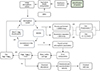 |
Fig. 1 Flow diagram showing the process sequence of SPECIES. Each step is explained in Sect. 2. The green box represents the beginning of the diagram. |
2.2 Equivalent width computation
The EWs were measured using the ARES code (Sousa et al. 2007, 2015). The input required by ARES is a one-dimensional spectrum and a line list. For each line, the code performs a local normalisation, over a window of 4 Å across the line centre. The normalisation is done by adjusting a third-order polynomial to that portion of the spectrum, and selecting only the points laying above rejt times the obtained fit. This process is repeated three times, and the final local continuum is subtracted from the data. rejt is computedper spectrum, and depends on the signal-to noise (S/N) of the data, where large (~1) values would correspond to high S/N. We use the S/N given in the image header, and when that is not provided, we compute it as the median of the S/N for different portions of the spectra, free of absorption lines. More information about this parameter can be found in Sousa et al. (2007). For the computation of the atmospheric parameters, we only consider lines with EWs in the range 10 ≤ EW ≤ 150 mÅ, in order to avoid lines too weak that could be affected by the continuum fitting, and lines too strong for which the LTE approximation might no longer be valid. We also discarded the lines for which σEW ∕EW > 1, where σEW is the error in the EW measured with ARES. We note that for these rejected lines, the Gaussian fit performed by ARES is not accurate enough, leading to an incorrect computation of the stellar parameters. We also perform a restframe correction in all our spectra before computing the EW of the lines. This was done by cross-correlating (Tonry & Davis 1979) a portion of the spectrum, between 5500 Å and 6050 Å, with a G2 binary mask within the same wavelength range. The wavelength was then scaled as λ = λo∕(1 + v∕c), where λo is the observed wavelength, v is the derived velocity of the star that SPECIES computes using a cross-correlation method, and c is the speed of light. This spectrum will be used for the rest of the calculations. One example of this cross-correlation function (CCF) and subsequent velocity correction is shown in Fig. 2. We have made sure that the instruments accepted by our code have a wavelength coverage that is wide enough so that the region of the spectra used for the restframe correction is included.
2.3 Initial conditions
Initial values for the atmospheric parameters (Teff, log g, [Fe/H]) are needed for their subsequent derivation through SPECIES, in a manner which will be explained in the next section. The initial conditions can be input by the user, or can be derived from the photometric information for each star.
In the case that the photometric magnitudes are retrieved from existing catalogues, they first should be corrected for interstellar extinction. We use the coordinates and parallax, along with the Cardelli et al. (1989) extinction law, and RV = 3.1, to obtain the extinction in the V -band, AV for each star using the Arenou et al. (1992) interstellar maps. Extinction in the rest of the photometric bands, Aλ, was derived from the Cardelli et al. (1989) relations. The corrected magnitudes for each band is then obtained as mλ,C= mλ,O − Aλ, where mλ,O is the magnitude retrieved from the catalogue, and mλ,C is the extinction corrected magnitude.
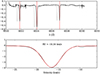 |
Fig. 2 Restframe correction applied to HD 10700. Top panel: Original spectra (grey), corrected spectra (black), and three reference lines at 6021.8, 6024.06, and 6027.06 Å (red). Bottom panel: Cross-correlation function (CCF) between the binary mask and the spectra. The red line corresponds to the Gaussian fit to the CCF, with a mean equal to −16.54 km s−1. |
2.3.1 Luminosity class
Before deriving the initial conditions, it is necessary to classify the star as a dwarf or giant. That is done by using the JHK magnitudes, and the intrinsic colours of dwarfs and giants, for different spectral types, from Bessell & Brett (1988). We first converted the JHK magnitudes to the Bessel and Brett system using the relations from Carpenter (2001)3. We then computed the distance to the dwarf and giant evolutionary models, and classify the star from the curve for which the distance is the shortest. This procedure, as well as the dwarf and giant curves from Bessel and Brett, are shown in Fig. 3. If the JHK magnitudes are missing, the star is classified as a dwarf. This procedure is also performed only when H − K > 0.14, which is when the dwarf and giant curves no longer overlap. For stars with H − K < 0.14, they are classified as dwarfs.
2.3.2 Metallicity
The metallicity is derived from Eq. (1) of Martell & Laughlin (2002), using the Strömgren coefficients b − y, m1, and c1. This relation is valid for − 2.0 < [Fe∕H] < 0.5. In the case the Strömgren coefficients are missing, or the derived metallicity is outside of the permitted ranges, then [Fe/H] is set to zero.
2.3.3 Temperature
The derivation of the initial effective temperature (Tini) will depend of the luminosity class. In the case of dwarf stars, the photometric relations from Casagrande et al. (2010, hereafter C10) or Mann et al. (2015, hereafter M15) are used. The difference between both relations is that the one from M15 is optimised for M dwarf stars, and the relations from C10 are applicable for FGK stars. In order to infer which type of star we are dealing with, we use its apparent magnitudes and the intrinsic colours for each spectral type derived in Pecaut & Mamajek (2013, hereafter P13). If the colours are in agreement with a K07 star or later, we use the M15 relations. If the photometric colours are outside of the permitted ranges for the C10 or M15 relations, we then infer the initial temperature by interpolating from the photometric colours and temperatures from P13. The colour in different bands and temperatures, along with the spline representation of each curve, are shown in Fig. 4.
In C10, M15 and P13, several relations are available for different photometric colours. For each star, we compute the average of the temperature derived for each photometric colour, weighted by their uncertainty.
If the star is classified as a giant, then the relations from González Hernández & Bonifacio (2009) are used. Just like for C10 and M15, different temperatures are derived for each photometric colour, and the final value corresponds to the average of the individual temperatures for each colour, weighted by their uncertainty.
The initial temperature will also set the boundaries of the parameter space through which SPECIES will search for the final temperature. These boundaries are set to be 200 K from Tini. In Sect. 3.1 we will show the reasons for choosing 200 K as the window over Tini. This can be disabled by the user at any time.
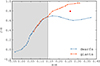 |
Fig. 3 Intrinsic JHK colours for dwarf (blue line) and giant (red line) stars, from Bessell & Brett (1988). The red point represents a star with H − K = 0.26 and J − H = 0.79. The distance between the point to the giant curve is 0.08 dex, and to the dwarf curve is 0.13 dex, therefore the star is classified as giant. The shaded area represents the H − K range for which the curves overlap, and no classification can be correctly performed. In those cases, the star is classified as dwarf. |
2.3.4 Surface gravity
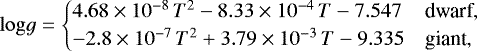
The initial surface gravity is derived by comparing log g and Teff obtained for stars in the literature with different luminosity classes. We used the sample of stars from the NASA Exoplanet Archive4, and separated the points into two classes: dwarf (log g ≳ 4.0) or giants (log g ≲ 4.0). Then, we adjusted a second order polynomial to each group, obtaining the following relations, depending on the luminosity class:
 (1)
(1)
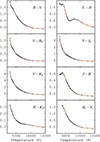 |
Fig. 4 Photometric colours of main sequence stars, for different effective temperatures, from Pecaut & Mamajek (2013). Red lines represent the spline approximation for each curve. The temperature for a given colour is computed as the root of the (m1 − m2) − (m1,⋆ − m2,⋆) curve, wherem1 − m2 is the chosencolour, and m1,⋆, m2,⋆ are the star’s colours. |
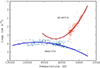 |
Fig. 5 logg vs. temperature for several stars in the literature. Red points represent giant stars, and blue points dwarf stars. The solid lines are the polynomials adjusted to each group, showed in Eq. (1). |
2.4 Atmospheric parameters
The atmospheric parameters (Teff, log g, [Fe/H], and ξt) are derived using equivalent widths (EWs) for the set of Fe I and Fe II lines discussed above. These EW values, along with an appropriate atmosphere model obtained by interpolating through a grid of ATLAS9 atmosphere models (Castelli & Kurucz 2004), are given to the 2017 version of the MOOG code (Sneden 1973), using the driver abfind, which solves the radiative transfer equation assuming local thermodynamic equilibrium (LTE) conditions. The atmospheric parameters are then derived through an iterative process that stops when no correlation is found to a tolerance level of 0.02 dex between the abundance of each individual Fe I line and both the excitation potential and the reduced equivalent width (log EW∕λ), and also when the average abundances for Fe I and Fe II are equal to the iron abundance given to the atmosphere model at the level of 0.02%.
The ranges in parameters accepted by the code are [3500–15 000 K] for the temperature, [−3.0–+1.0 dex] for the metallicity, [0.0–5.0] for the logarithm of the surface gravity in cm s−2, and [0.0–2.0 km s−1] for the microturbulent velocity. If, during the iterative process, all four parameters are outside of those ranges, or the same values are repeatedmore than 200 times, the computation stops. This last case would mean that SPECIES is stuck in one section of the parameter space, prolonging the time the code runs, without reaching final convergence. From our experience using SPECIES, we find that after the same parameters are repeated over 200 times, the code is not able to search the rest of the parameters space. For those cases, it is recommended that the user specifies the initial conditions, or fixes one of the parameters to a certain value. If no convergence was reached, we perform the derivation another time but now setting the temperature to be equal to Tini, and keeping it fixed. SPECIES also has an option to set the microturbulence to a fixed value through the computation. We found that, for some stars, all the atmospheric parameters would reach convergence except for the microturbulence, therefore for those stars we set ξt = 1.2 km s−1. These options to fix the temperature or/and the microturbulence are only used when there was no convergence on the atmosphericparameters, and can be disabled by the user.
2.5 Uncertainty estimation
An important facet of the SPECIES code is the handling of uncertainties for each of the calculated parameters. A number of the parameters derived by SPECIES are heavily correlated, such as temperature and iron abundance, due to them being derived simultaneously with MOOG via the curve of growth analysis. The code tries to take into consideration these correlations to return a more representative uncertainty estimate for each of the elements, and to consider the uncertainty in the EW (derived with ARES) in the equation. In order to do so, we took as a reference the uncertainty estimation method used in Gonzalez & Vanture (1998) and Santos et al. (2000). In Table 1 we show the typical uncertainties obtained for each atmospheric parameter, separated in ranges of stellar temperature.
2.5.1 Microturbulence
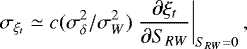
The microturbulence is computed as the value for which the slope of the linear fit performed between the individual FeI abundances and the reduced equivalent width reaches zero. This value will be referred to as SRW. Therefore, the resulting uncertainty will depend on this slope, resulting in:
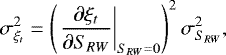 (2)
(2)
where  corresponds to the uncertainty in SRW.
We computed this uncertainty for 160 stars from the sample studied in Sousa et al. (2008), and for 10 solar spectra, all taken using HARPS (more details about this sample of stars will be given in Sect. 3.2). We found that, for each case, there was a dependency of ξt with SRW, which can be adjusted with a cubic spline,
 (3)
(3)
where Y represents a cubic spline, with coefficients vi. The coefficients are a function of microturbulence velocity, shown in Fig. 6, and have the following dependence:
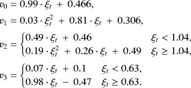 (4)
(4)
Another way SPECIES computes the uncertainty in the microturbulence is explained in the appendix, and although we performed this method on all our stars, it is not the preferred final value. We note however that it does appear in the SPECIES catalogue aserr_vt2.
Estimate of the uncertainties for the stellar parameters, separated in ranges of stellar temperature, for dwarf stars.
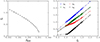 |
Fig. 6 Top panel: ξt vs. SRW for a Solar spectrum. Bottom panel: fit of the spline coefficients as a function of microturbulence. |
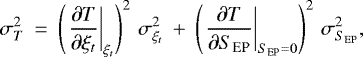
2.5.2 Temperature
The temperature is obtained when the slope of the dependence between the individual Fe I abundances, and the excitation potential, is zero. We will call this slope as SEP. Since all theatmospheric parameters are derived simultaneously, the microturbulence will have an effect on the final temperature, and its uncertainty. The final expression for the error in the temperature is then:
 (5)
(5)
where ∂T∕∂ξt is evaluated at the microturbulence derived by our code,  is its uncertainty, and
  is the uncertainty in SEP, when the temperature reaches convergence.
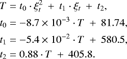
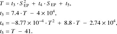
In order to find the first term, we computed the value of the temperature after fixing ξt to a specific value. We obtained a quadratic fit, which is shown in the top-left panel of Fig. 7. For the second term, we followed a similar procedure to the one discussed for the microturbulence, and computed the temperature we would obtain as a function of SEP. In this case, the dependence could be fitted by a quadratic curve, and is shown in the top-right panel of Fig. 7.
As we did before, to find the values for the coefficients of the dependence between T and ξt, and between T and SEP, we computed the uncertainties for the same sample of stars than in the previous section. The coefficients corresponding to the relation between T and ξt are plotted in the bottom-left panel of Fig. 7, and depend on T in the following way:
 (6)
(6)
For the relation between T and SEP, the coefficients are plotted in the bottom-right panel of Fig. 7, and have the following dependency with T:
 (7)
(7)
Again we highlight a second way to compute the uncertainty in temperature that is explained in the appendix. We performed it for all our stars but it is used mainly as a cross-check and is again not the preferred value. It appears in the catalogue as err_T2.
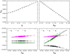 |
Fig. 7 Top panel: dependence of temperature with microturbulence (left) and SEP (right), for a Solar spectrum. Bottom panel: coefficients of the fit between T and ξt (left), and between T and SEP (right). |
2.5.3 Metallicity
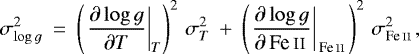
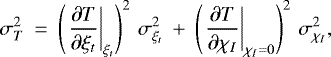
The final value for the metallicity is reached when the average of the individual Fe I abundances matches the one from the input model atmosphere, and will depend on the scatter found in the Fe I abundances. As was mentioned previously, the final metallicity will also depend on the rest of the atmospheric parameters, and in this case, it will depend on the temperature and the surface gravity. The final expression for the uncertainty in the metallicity will be:
![Mathematical equation: \begin{equation*} \sigma_{\text{[Fe/H]}}^2 \: =\: \left(\left.\frac{\partial \text{[Fe/H]}}{\partial \xi_t}\right|_{\xi_t}\right)^2\, \sigma_{\xi_t}^2 \: +\: \left(\left.\frac{\partial \text{[Fe/H]}}{\partial T}\right|_{T}\right)^2\, \sigma_{T}^2 \: +\: \sigma_{\text{Fe\,\textsc{i}\,}}^2, \end{equation*}](/articles/aa/full_html/2018/07/aa31533-17/aa31533-17-eq11.png) (8)
(8)
where ∂[Fe/H]∕∂ξt and ∂[Fe/H]∕∂T are evaluated at ξt and T derived by our code, respectively, and σFe I is the scatter over the abundances of each Fe I lines.
We computed the metallicity for different values of the temperature and microturbulence, and obtained the following relation:
![Mathematical equation: \begin{equation*} \text{[Fe/H]}\: =\: (m_0\cdot \xi_t + m_1)\cdot T \: +\: (m_2\cdot \xi_t + m_3), \end{equation*}](/articles/aa/full_html/2018/07/aa31533-17/aa31533-17-eq12.png) (9)
(9)
which can also be seen in the top panels of Fig. 8.
We followed the same procedure than in the previous sections to find the dependence of the fit coefficients with the metallicity. The fits we obtained are plotted in the bottom panel of Fig. 8, and correspond to
![Mathematical equation: \begin{align*}m_0& = 2.02\times 10^{-5}\cdot \text{[Fe/H]} \: -\: 1.8\times 10^{-5}, \nonumber \\ m_1& = -9.57\times 10^{-5}\cdot \text{[Fe/H]} \: +\: 7.03\times 10^{-4},\\ m_2& = -0.2\cdot \text{[Fe/H]} \: -\: 0.04, \nonumber \\ m_3& = 1.49\cdot \text{[Fe/H]} \: -\: 4.01. \nonumber \end{align*}](/articles/aa/full_html/2018/07/aa31533-17/aa31533-17-eq13.png) (10)
(10)
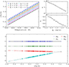 |
Fig. 8 Top panel: (left) dependence of metallicity with temperature for several values of microturbulence, (right) dependence of the coefficients a and b with ξt, so that [Fe/H] = a ⋅ T + b. Bottom panel: coefficients of the fit of [Fe/H] with T and ξt, so that a = m0 ⋅ ξt + m1 and b = m2 ⋅ ξt + m3. A vertical offset was applied to each coefficient for plotting purposes. |
2.5.4 Surface gravity
The surface gravity depends on the average abundance obtained for the Fe II lines, as well as on the final temperature from the iterative process. Therefore, the uncertainty in log g will be given by:
 (11)
(11)
where ∂logg∕∂T and ∂logg∕∂ Fe II are evaluated for T and [Fe/H] found by our code, respectively.
As for the previous parameters, we found that logg = l0 ⋅ Fe II + l1, and logg = l2 ⋅ T2 + l3 ⋅ T + l4. Both of these relations are plotted in the top panel of Fig. 9. The coefficients l0, l1, l2, l3, and l4 all depend on the temperature and are shown in the bottom panel of Fig. 9. The relations and coefficient values are as follows:
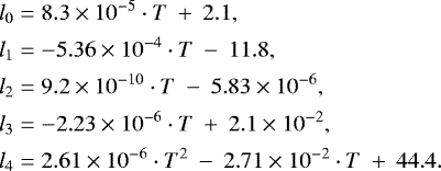 (12)
(12)
2.6 Mass, age, and radius
SPECIES uses the python package isochrones5 (Morton 2015) in order to derive the mass, age, and radius for each star. It uses the previously derived [Fe/H], log g, and Teff, and the MESA Isochrones and Stellar Tracks (MIST; Dotter 2016). The package performs a MCMC fit, with priors given by the [Fe/H], logg, and Teff input values, plus their uncertainties. The samples generated correspond to the mass, age, and radius, evaluated at each chain link. The resulting values will be given by the median and standard deviation of the posterior distributions. It is also possible to input photometric data as priors. This data corresponds to apparent magnitude in several bands, as well as parallax in mas, and can either be given by the user, or retrieved from catalogues. The list of catalogues used, as well as the allowed magnitudes, are given in Sect. 2. Figure 10 shows an example posterior distribution obtained for one of our solar spectra.
Another value measured from the isochrones interpolation is the surface gravity a star would have for themass, age, and radius derived previously. This quantity, which we will referred to as log giso, should match the input logg (referred to as the spectroscopic logg within the text), and it does so in most cases, but we do find some exceptions. When using SPECIES on a sample of dwarf stars (which will be further explained in Sect. 3.2), we find that for some cases the value of log g is <4.0. We also find better agreement between loggiso and the surface gravity from the literature (for the description of the catalogues used for the comparison, see Sect. 3.2), than when using the spectroscopic logg (Sect. 3.2.1, Fig. 18). This leads us to conclude that log giso is a better tracker of the true surface gravity than the logg obtained from the iterative process explained in Sect. 2.4. In order to incorporate this result into the computation, we studied the distribution of log g – loggiso (Fig. 11), and we found that it follows a Gaussian distribution centred around zero, and with a standard deviation equal to 0.11. Most of the stars are found contained within 2σ of this distribution. For the cases when the discrepancy between both logg measurements is larger than 2σ, which translates into 0.22 dex, we perform a second iteration to derive the atmospheric parameters, following the same procedure than in Sect. 2.4, but setting log g = log giso as the correct value. This option can be disabled when running SPECIES (Sect. 3).
It is important to mention that loggiso not only seems to provide a better estimate of the true surface gravity of a dwarf star, but it also agrees for evolved stars. This is shown in Sect. 3.2.3, where we use SPECIES to derive the parameters for a sample of dwarf and evolved stars, and we find agreement between our values and those from the literature.
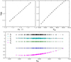 |
Fig. 9 Top panel: (left) dependence of surface gravity (logg) with individual Fe II abundance, (right) dependence of logg with temperature. Bottom panel: coefficients of the fits between logg with Fe II, and between logg with Teff, as shown in Eq. 12. A vertical offset was applied to each coefficient for plotting purposes. |
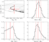 |
Fig. 10 Results obtained for one of the solar spectrum used in SPECIES. First panel: log g –Teff space diagram. The red point represents the position of the Sun, with the final values obtained using our code (T = 5776 ± 73 K, [Fe/H] = 0.0± 0.1 dex, logg = 4.5 ± 0.2 cm s−2). Dotted lines represent the evolutionary tracks for stars with masses from 0.5 to 1.5 M⊙, and [Fe/H] = 0.0. The black line is the track for a 1.0 M⊙ star. Each point in the lines represent a different age. Remaining panels: distribution of the mass, age, and radius, for one of our HARPS solar spectra. The red dashed-solid-dashed lines represent the (16, 50, 84) quantiles, respectively. The results for this spectrum are listed in Table 3 as sun03. |
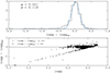 |
Fig. 11 Top panel: histogram of the difference between logg and log giso. The blue line corresponds to the Gaussian distribution fit performed, with mean and sigma equal to μ = −0.004 and σ = 0.112, respectively. Bottom panel: difference between logg and log giso vs log g. Filled circlesare the stars laying within 2σ of the Gaussian fit performed to the histogram. Empty circles are the points laying beyond the 2σ level, for which the computation was performed a second time, but setting log g = log giso. |
2.7 Chemical abundances
SPECIES allows the computation of chemical abundances for 11 elements (Na, Mg, Al, Si, Ca, Ti, Cr, Mn, Ni, Cu, Zn) and to test the level to which the code performs these measurements, we compared the SPECIES values with the solar values already studied in the literature, where we used the values for Teff, log g, [Fe/H], and ξt computed previously. We used the line list used in Ivanyuk et al. (2017; we refer the reader to that work for a detailed description of the line selection), and the solar abundances from Asplund et al. (2009). The EW were measured using the ARES code, and for the analysis only lines with 10 < EW ≤ 150 were used, as explained before.
For each element, we considered only the lines for which the individual abundance was within 1.5σ of the mean value. This was done in order to avoid the lines that deviate too much (more than 2 dex in some cases) from the abundance given by the rest of the lines for that element. The final abundance for each element was computed as the average abundance from each individual line, after the sigma-clipping, and its uncertainty was taken as the standard deviation over the average. We weighted the abundance of each line as 1/σEW. When only one line per element is available, the uncertainty is taken to be the average error for the other elements used, and no sigma-clipping was performed.
For all the elements, except for Ti, only lines from neutral species were used. In the case of Ti, we list the abundances obtained for both Ti I and Ti II. We also include in the output the abundances for Fe I and Fe II.
Currently, it is not possible to quickly modify the line list, nor add new species to the computation.
2.8 Macroturbulence and rotational velocity
In order to compute the macroturbulence (vmac) and rotational (vsini) velocities, we followed the procedure described in dos Santos et al. (2016). It consist of measuring both quantities individually for five different absorption lines, and then compares the results to those from the Sun. The lines used, as well as their atomic characteristics, are mentioned in Table 2.
The macroturbulent velocity was obtained from dos Santos et al. (2016, Eq. (1)):
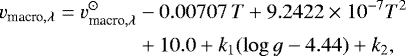 (13)
(13)
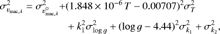
where  are the velocities obtained for each line in the solar spectra, shown in Table 2. k1 and k2 are constants equal to −1.81 ± 0.26 and −0.05 ± 0.03, respectively. All the quantities mentioned were computed by dos Santos et al. (2016). This relation is also very similar to the one used in Valenti & Fischer (2005). The uncertainty in vmac,λ for each line is given by:
 (14)
(14)
where the error in  is reported to be ±0.1 km s−1. The temperature and surface gravity, along with their uncertainties, are the ones produced by SPECIES. The final vmac corresponds to the average of the individual results, weighted by their uncertainties.
The rotational velocity for each line was obtained by comparing the line profiles with synthetic ones produced by the MOOG driver synth. The driver receives a model atmosphere, obtained from the ATLAS 9 grids and the atmospheric values found by SPECIES, and the line abundance, found by measuring the EW of the line with ARES (following the same settings described in Sect. 2.2), and using the MOOG driver abfind. It also receives the macroturbulent velocity found previously, and the width of the line produced by the instrument resolution. The synthetic profile is then convolved with a rotational profile (Gray 2005) for a certain v sini value. This was performed using the PoWeRS6 code, which was modified and optimised in order to fit into SPECIES. The code creates grids of different values for v sini and line abundance, and finds the values (abundance, vsini) for which the synthetic profile best matches the original line profile. This is measured by the quantity S, which measures the goodness of the fit, and is given by
 (15)
(15)
with i = {0, ..., N} the number of points in the line profile, which is considered from λ − 0.5 to λ+ 0.5. yo represents the measured line profile, and ys the synthetic one. The code performs a cubic spline fit to the value of S vs. the abundance and rotational velocity, and finds the values for which the minimum of S is reached. A minimum of four iterations are performed, refining the abundance and velocity grids by shifting the grid centre to match the values with the best goodness of fit, and making the delta between grid points smaller. This is done in order to obtain the most precise results (minimum of S). In Fig. 12 we show the changes in S for a grid of line abundances and rotational velocities, and the final fits obtained for each line, for a solar spectrum. The final vsini corresponds to the average of the individual values found for each line, and its uncertainty is estimated as  , where the sum is performed over all the lines.
The stellar parameters obtained for the Sun, using 10 different solar spectra taken with the HARPS instrument7, are listed in Table 3. The final values found, after performing a weighted average with the S/N of each solar spectrum, are T = 5754.2 ± 23.3 K, [Fe/H] = −0.02 ± 0.02 dex, log g = 4.38 ± 0.05 cm s−2, ξt = 0.68 ± 0.11 km s−1, vmac = 3.15 ± 0.06 km s−1, v sini = 2.35 ± 0.27 km s−1, mass = 0.96 ± 0.01 M⊙, radii = 1.00 ± 0.01, and age = 6.17 ± 0.7 Gyr.
Line list used to measure the rotational velocity for each star.
3 Results obtained with SPECIES
Currently, the SPECIES catalogue has 72 columns with the stellar parameters, described in Appendix D. In order to test the accuracy of the results obtained with SPECIES, we derived the parameters for a sample of 584 dwarf stars, targeted by the HARPS GTO projects (parameters derived in Sousa et al. 2008) and the Calan-Hertfordshire Extrasolar Planet Search (CHEPS) programme (Jenkins et al. 2009, stellar parameters derived in Ivanyuk et al. 2017). They cover a wide range in temperature and metallicity, from 4300 to 6500 K, and −0.9 to 0.6 dex, respectively. We selected the highest S/N spectra taken with HARPS (given that it is the highest resolution instrument currently accepted by SPECIES), and compare them with what is obtained with photometric relations and other catalogues in the literature. Unless stated otherwise, the results presented here were computed using the temperature from photometry and/or fixing ξt = 1.2 km s−2 when convergence is not reached in the atmospheric parameters, and setting log giso as the correct value for the surface gravity when their differences are larger than 0.22 dex. If different options were used in the computation, it will be specified within the text and in the captions of the figures and/or tables. A sample of the catalogue is shown in Table D.1.
3.1 Comparison with photometric relations
The first comparison we performed was to analyse the differences between the temperatures derived from our code and from the photometric relations explained in Sect. 2.3.3. As was mentioned in Sects. 2.3.3 and 2.4, we used the temperatures derived from photometry (for the cases when that information was available) as an initial value for SPECIES, and in the cases when our code could not converge to a valid result for the atmospheric parameters.
In orderto check that the temperature from photometry is in agreement with that from SPECIES, we compared both results for our sample of FGK dwarfs stars, observed with HARPS, FEROS, HIRES, and UVES. We considered only the cases when it was not necessary to set the temperature from photometry as the correct value to reach converge in the derivation of the atmospheric parameters. For each star we retrieved the photometric information from Vizier, using the catalogues mentioned in Sect. 2, and computed the temperature using the relations from Sect. 2.3.3.
We computed the difference between the temperature from SPECIES, and from using each photometric relation, for spectra taken with different instruments. We then adjusted Gaussian models to the distributions obtained, and define the mean of the model as the offset between each temperature measurement. This was done for every relation described in Sect. 2.3.3, except when using González Hernández & Bonifacio (2009), due to the small number of stars in our sample which met the requirement of being classified as giants. Instead of adjusting Gaussian models to the distribution, we just computed the mean of the difference, setting that value as the offset between both temperature measurements. The results from the comparisons are shown in Figs.13–15, and Tables 4–6, for the relations from Casagrande et al. (2010), Mann et al. (2015), and Pecaut & Mamajek (2013).
We use these offsets to correct the temperatures obtained using the photometric relations (Sect. 2.3.3), to match the values with those obtained by SPECIES. For the case of the relations from González Hernández & Bonifacio (2009), we did not perform this comparison because we had no giants in our test.
Finally, we compared the final metallicity, surface gravity and temperatures obtained with SPECIES, and the initial values derived from photometry in Sects. 2.3.2, 2.3.4, and 2.3.3. The distributions we obtain for the difference between both quantities are shown in Fig. 16. For all three parameters we find them to be distributed around zero (median of the distributions around −0.0001 and 0.02 for the metallicity and surface gravity, respectively), meaning excellent agreement. We find only a few cases that the values from SPECIES are smaller than from the photometric relations.
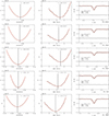 |
Fig. 12 Change of S versus abundance (left panels) and rotational velocity (middle panels), for each line of the solar spectra. The red lines represent the cubic spline fit performed over the data, and the vertical line shows the values where the minimum of S is reached. Right panels: line profiles, along with the final fit (red line) combining the instrumental profile, macroturbulence and rotational velocity. The horizontal black line around zero represents the residuals of the fit. |
Stellar parameters found for a sample of Solar spectra, taken using HARPS.
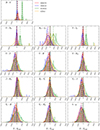 |
Fig. 13 Histograms of the difference between the temperature computed by SPECIES, and those using the colour relations from C10. The lines correspond to Gaussian distributions adjusted to the histograms, with mean values listed in Table 4. Each colour represents a different instrument: red for HARPS, blue for FEROS, green for HIRES, and orange for UVES. The different panels show the temperatures computed using different photometric colours, mentioned in Sect. 2. |
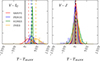 |
Fig. 14 Histograms of the difference between the temperature computed by SPECIES, and by using the colour relations from M15. The lines correspond to the Gaussian fits for each distribution, and the colours represent the same instruments as in Fig. 13. The mean of the Gaussian fits are shown in Table 5. |
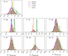 |
Fig. 15 Histograms of the difference between the temperature computed by SPECIES, and those obtained by interpolating through the models of P13. The lines correspond to Gaussian distributions adjusted to the histograms, with mean values listed in Table 4. The mean of each Gaussian distribution is listed in Table 6. The colours represent the same instruments as in Fig. 13. |
Mean of the Gaussian fits (in K) performed on the distribution of differences between the temperatures derived by SPECIES, and from using the colour relations from C10.
Mean of the Gaussian fits (in K) performed on the distribution of differences between the temperatures derived by SPECIES, and from using the colour relations from M15.
3.2 Comparison with other catalogues
In order to test the accuracy of SPECIES, we compared the spectral parameters for a set of stars obtained with our code, with ones listed in the literature. We chose five different catalogues for this comparison, since each had analysed a large sample of stars and they all used differing methods to compute the stellar parameters, providing a robust test of the SPECIES automatic calculations. The samples are briefly described as follows:
Brewer et al. (2016, hereafter SPOCS2), a continuation of Valenti & Fischer (2005, SPOCS), in which stellar parameters were presented for ~1000 stars. They used the spectral synthesis method to derive the atmospheric parameters, and interpolation using Yonsei-Yale (Y2) isochrones (Demarque et al. 2004) to obtain mass and age measurements. They set the microturbulence velocity to 4 km s−1 through their calculation, and derive a formula for the macroturbulence velocity very similar to the one used in this work (Eq. (13)). In SPOCS2, the abundances list was increased, as well as the number of stars in their sample (~1600 stars).
Sousa et al. (2008, hereafter S08), in which they used the same method as we did to compute the atmospheric parameters (Teff, logg, [Fe/H], and ξt), that is by computing the EWs using ARES for a set of iron lines and then using MOOG to derive their stellar parameters. In the case of the abundances for other chemical elements, we used the values from Adibekyan et al. (2012, hereafter A12), which uses the atmospheric parameters derived in S08.
Bond et al. (2006, hereafter B06), where the procedure used to derive their parameters also relied on the measurement of EWs, assuming LTE to derive the atmospheric parameters. There are considerable differences between their method and ours. First, they measured the EWs of their lines by direct integration, instead of Gaussian fitting, as is done in this work. Second, the temperatures were derived using the star colours, following the relation from Smith (1995). Finally, they derived the metallicity with two different methods, one using Strömgren uvby colours (Strömgren 1966), and the other using the measured EW. For this comparison, we are using the metallicity values derived through spectroscopy.
Bensby et al. (2014, hereafter B14), in which they also used EW measurements, along with LTE model stellar atmospheres, in order to determine the parameters. The differences between their method and ours are that in B14 they used the MARCS code (Gustafsson et al. 1975) to solve the radiative transfer equations, computed the EW for each lineusing the IRAF task SPLOT, and used Y2 isochrones to derive the mass and age of each star.
Ivanyuk et al. (2017, hereafter I17), where they used the Infrared Flux Method (IRFM; Blackwell & Lynas-Gray 1994) calibration to derive effective temperatures, and the modified numerical scheme developed by (Pavlenko 2017) in order to compute the iron abundance, surface gravity, microturbulent and rotational velocity, from high S/N HARPS spectra observed as part of the Calan-Hertfordshire Extrasolar Planet Search (CHEPS) programme (Jenkins et al. 2009). These values were then used to derive the atomic abundances for several elements.
We selected the highest S/N spectra taken with HARPS (given that it is the highest resolution instrument currently accepted by SPECIES) for each star we wanted to analyse, which left us with 95 stars for SPOCS2, 435 stars for S08, 67 stars for B06, 99 stars for B14, and 103 stars for I17
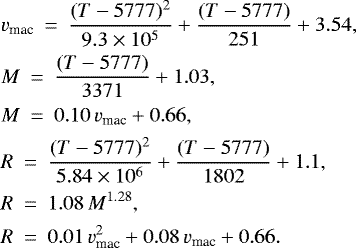
The comparison between the atmospheric parameters (plus mass and age) from each catalogue and ours are shown in Fig. 17. In Fig. 19 the same comparison is shown for the chemical abundances (only the elements we had in common with each catalogue).
Mean of the Gaussian distribution (in K) adjusted to the histograms of the different between the temperature from SPECIES, and from interpolating between the models of P13.
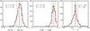 |
Fig. 16 Histograms of the difference between the metallicity (left panel), surface gravity (middle panel) obtained with SPECIES, and from using the photometric relations from Sects. 2.3.2 and 2.3.4 (right panel). The vertical lines correspond (from left to right) to the 16, 50 and 84 percentiles. |
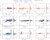 |
Fig. 17 Comparison between the values for different parameters obtained with our code and from literature. The y-axis in the plotscorrespond to the difference between both measurements, represented by different symbols and colours: blue circles to Sousa et al. (2008), red triangles to Brewer et al. (2016), green diamonds to Bond et al. (2006), orange squares to Bensby et al. (2014), and cyan stars to Ivanyuk et al. (2017). The black points in the bottom right of each plot represents the average uncertainty in the points. The histograms in the right panels of each of the plots show the distribution of the results, fitted by Gaussian functions, with parameters given in Table 7. |
Parameters of the Gaussian distributions adjusted to the difference of stellar parameters from SPECIES and from the literature.
Parameters of the Gaussian distributions adjusted to the difference of atomic abundance from SPECIES and from the literature.
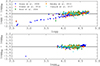 |
Fig. 18 Comparison between the surface gravity from SPECIES, and from the literature. In the top panel, the surface gravity from SPECIES corresponds to the results obtained from the convergence of the atmospheric parameters (Sect. 2.4), without the option of recomputing using log giso. In the bottom panel, the surface gravity from SPECIES corresponds to the log giso obtained forthe same stars (Sect. 2.6). |
Gaussian distribution parameters (μ, σ) obtained for the difference between stellar parameters from HARPS, and from other instruments.
Gaussian distribution parameters (μ, σ) obtained for the difference between atomic abundances from HARPS, and from other instruments.
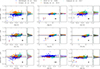 |
Fig. 19 Comparison between the abundances for different elements obtained with our code and from literature. The y-axis in the plotscorrespond to the difference between both measurements, represented by different symbols: blue circles to Sousa et al. (2008), red triangles to Brewer et al. (2016), green squares to Bond et al. (2006), orange squares to Bensby et al. (2014), and cyan stars to Ivanyuk et al. (2017). The black points in the bottom right of each plot represents the average uncertainty in the points. The histograms at the right panels of each plots show the distribution of the results, fitted by Gaussian functions. |
3.2.1 Fundamental physical parameters
In order to study the agreement between our results for the fundamental parameters (Teff, [Fe/H], log g, ξt, v sin i, vmac, mass, age, and radius), with that of the literature, we computed the difference between both measurements, obtaining for each parameter and catalogue a distribution of differences around zero. Then, for each distribution we adjusted a Gaussian function obtaining the mean (μ) and standard deviation (σ) of the difference of results. For the analysis performed in the following sections, we consider the mean of the distribution as the offset between our results and the literature, and the significance of that offset will be given by the width of the distribution, and how far away from zero it is located. The difference in parameters, as well as the adjusted Gaussian distributions, are shown in Fig. 17, and the Gaussian parameters (μ, σ) are shown in Table 7.
We find that, overall, the measurements are in good agreement (μ ≤ 1.5σ) among the different catalogues, albeit with a few exceptions. These are found for the following quantities: for the temperature, μ = 1.55σ against I17. For the metallicity, μ = 1.80σ and 2.30σ against the values from B06 and I17, respectively. For the microturbulence, we find μ = 1.89σ, 2.50σ, and 2.1σ against S08, B06, and I17, respectively. Finally, for the rotational velocity, we find that μ = 2.30σ for the distribution of our results against the ones from I17.
The largest discrepancies are found against the values from B06 and I17. Those catalogues are the only ones that only use photometric calibrations to derive the stellar temperatures (as explained above). In order to check if the temperature is the source of the discrepancies, we fixed the temperature to the values listed in B06 and I17, and then recomputed the rest of the parameters, for the stars we had in common with those catalogues. We find that, while the offsets with metallicity are significantly improved (0.0 and 0.04 with respect to B06 and I17, respectively), the other parameters do not improve. We conclude that the differences in temperature against what was obtained in B06 and I17 produce the offsets in metallicity, but are not responsible for the discrepancies with the rest of the parameters. The results for the rotational velocity are also very different between SPECIES and I17. The SPECIES results are smaller than for I07, except for very few exceptions. We believe this is caused by considering the line broadening as the contribution from rotational and macroturbulence velocities, instead of taking into account only the rotational contribution (as was done in I07). This manifests into lower rotational velocities than in I07.
As for the offsets seen with the other catalogues, these can be due to the different method and calibrations used to derive the parameters, and can be corrected with respect to the ones obtained with SPECIES by applying the values in Table 7.
We looked again at the differences with logg and loggiso. In Sect. 2.6, we stated that loggiso (the surface gravity a star would have for the mass, age and radius derived from isochrones) is a better indication of the true log g than the spectroscopic value. We now compare the surface gravities from the literature against those that SPECIES would obtain without the option to recompute the stellar parameters with log g = log giso, and against loggiso. This is shown in Fig. 18. We obtain large discrepancies between log g and the literature for logg < 4.0, but this difference disappears when using the loggiso value. This supports the statement we made in Sect. 2.6, that log giso is a better representation of the true surface gravity of a star in a lot of cases. SPECIES will use log giso as the correct results for the cases when log g - loggiso > 0.22 dex.
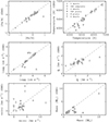 |
Fig. 20 Results for the stellar parameters, obtained with SPECIES (x-axis), compared with what was found in the literature (y-axis), for the GBS sample. The different symbols denote different spectral types. The dashed line represents the 1:1 relation. |
3.2.2 Atomic abundances
For the analysis of the atomic abundances from SPECIES, we followed the same procedure as in the previous section. We obtained the differences between the measurements from SPECIES and from the same catalogues already described and adjusted Gaussian distributions to the results. The results of this are shown in Fig. 19, and the parameters of the Gaussian distributions (μ, σ) are shown in Table 8. Different abundances for the sun were used as references in each of the works, so we first need to correct the results in the literature for the differences between their reference solar abundances and the scale used in this work (solar chemical composition from Asplund et al. 2009). We also remind the reader that the abundances for the S08 stars are listed in Adibekyan et al. (2012).
We find that the largest discrepancies are seen against the results of SPOCS2, and I17. For SPOCS2, μ = 1.86σ, 2.4σ, 3.5σ, 4σ, and 2.29σ for Na, Mg, Al, Ca, and Mn, respectively. For I17, μ = 5σ, 1.56σ, 1.56σ, and 2σ for Al, Ca, Ti, and Cr, respectively. We checked if the differences with I17 are again a consequence of the method they used to derive the temperature, by recomputing the abundances using the temperature from I17. We find a decrease in the offsets with respect to Ca and Ti (μ < 1.5σ), but almost no change in the results for Al and Cr. The improvement in the differences for some of the elements was expected, given that in the previous section we found that the discrepancy with the metallicity is significantly decreased when using the temperature from I17, which thus will affect the final chemical abundance. By seeing no improvement in Al and Cr, we can conclude that those elements are less affected by temperature and metallicity than the rest of the species analysed. We performed the same analysis but using the temperature from SPOCS2, to see if there are changes with the chemical abundance. We find that the discrepancies with Na and Mn decreases, falling below the 1.5 σ level, but for Mg, Al, and Ca we do not see such improvements, with the offsets still above the 1.5 σ level. This shows that differences in the temperature obtained between this work and SPOCS2 are not the source of the large abundance differences for Mg, Al, and Ca. I17 also compared their abundances against results from other catalogues (some of them included in this work) and even though they found similar trends in abundance vs. metallicity, they do see offsets between them. One of the explanations they find includes selection effects and differences in atomic line data.
Other large discrepancies we find are: μB14 = 2σB14 for Na, μB06 = 4.4σB06 for Al, μB06 = 2σB06 and μB14 = 2σB14 for Ca, and μA12 = 4.4σA12 for Mn. These can be explained by the differences in method used to derive the abundances, and differences in the line list used.
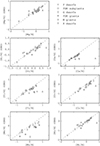 |
Fig. 21 Results for the chemical abundance of α and iron peak elements, obtained with SPECIES (x-axis), compared with what was found in the literature (y-axis), for the GBS sample. The different symbols denote different spectral types. The dashed line represents the 1:1 relation. |
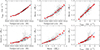 |
Fig. 22 Correlations between the stellar parameters computed by SPECIES. The red squares are the binned data points, and the blue lines correspond to the fits described in Eq. (16). The data used correspond to points within 3σ of their corresponding distribution. |
3.2.3 Results for the Gaia Benchmark Stars sample
Finally, we compared the results obtained with SPECIES for the Gaia Benchmark Stars (GBS) sample. This sample consists of 34 FGK stars, presented in Jofré et al. (2014), spanning a wide range of metallicities and gravities, which translates into different evolutionarystages.
The GBS sample was presented and studied in several works: Jofré et al. (2014) for the determination of metallicity, Heiter et al. (2015) for the effective temperature and surface gravity, and Jofré et al. (2015) for chemical abundance of α and iron peak elements. In those papers, the parameters for each star were computed using different methods (except for the rotational velocity, for which they extract values from the literature). The input spectra were obtained from Blanco-Cuaresma et al. (2014), and correspond to HARPS data. The results obtained with SPECIES for the GBS sample are shown in Fig. 20, for the atmospheric parameters, as well as rotational velocity and mass, and in Fig. 21 for chemical abundance. It is important to note that SPECIES could not converge to correct solutions for every star. Those corresponded, in most of the cases, to stars with very few spectral lines (mostly giant stars), or stars that are part of a spectroscopic binary system, where line blending was present in the spectra. The results obtained for each star are listed on Tables A.3 and A.4.
We find that the results from SPECIES are systematically larger than the ones from the literature, for all the parameters analysed. In term of the spectral types, we find good agreement with the FGK subgiant, giant, and G dwarf samples (mean of difference for each parameter between SPECIES and the literature is less than 1σ the mean uncertainty from SPECIES), with the exception of the mass and Mn abundance of FGK giants, where SPECIES obtained values larger than 1σ from the mean uncertainty. It is not possible to draw more conclusions for the other spectral types (F dwarfs, M giants, and K dwarfs), due to the low number of stars for each type (<3 stars for each case). We also looked at the log giso obtained forthe Gaia stars, and found them to be very similar to the surface gravity from Heiter et al. (2015). This favours the statement we made in Sect. 2.6 and 3.2.1, in which log giso is a good representation of the true logg for a lot of cases, now including stars in different evolutionary stages, with log g < 4.0 dex.
3.3 Correlation between parameters
We studied whether there were strong correlations between the stellar parameters, by plotting each quantity against the rest, considering only points within 3σ of the mean. We find that the majority of the parameters derived using this code show no strong correlations between each other, as can be seen in Fig. 26, even though we do find some exceptions. We find that the mass, radius, temperature and macroturbulent velocities show correlations among each other, as is shown in Fig. 22. We adjusted the following relations to those correlations:
 (16)
(16)
All these relations are shown as the blue lines in Fig. 22.
The mass correlation with temperature reflects the known mass–luminosity relationship for stars (Kuiper 1938), for which L ∝Mα. Dwarf stars increase in luminosity for higher temperatures, therefore the relation can be interpreted as larger mass for higher surface temperature. The correlation between macroturbulence velocity and temperature is produced by the method we used to derive vmac, following Eq. (13) (Sect. 2.8), and the increased depth of the convective envelope with decreasing temperature. In the equation for instance, the metallicity dependence is not as strong as the temperature dependence, which explains why we do not see such a strong correlation between macroturbulence velocity and metallicity (Fig. 26).
The relation between stellar mass and radius has been well studied over the years, and for main sequence stars, Demircan & Kahraman (1991) found that where R = 1.06 M0.945, for M < 1.66 M⊙. The fit we performed to the SPECIES results is in agreement with the previous relation.
The rest of the strong correlations seen in Fig. 22 are a consequence of the relations mentioned previously. The relation between mass and microturbulence is due to the relation between microturbulence and temperature, and of mass with temperature. The macroturbulence with microturbulence is also due to the relation between both quantities and temperature. Finally, the relation between macroturbulence and mass is produced by the effect temperature has on both parameters.
When looking at the chemical compositions, we studied its abundance with respect to iron, versus the star’s overall metallicity. This is shown in Fig. 23. We find that, for most of the elements, their abundance is greater than iron in metal-poor stars, and resembles (Mg, Al, Ca, Ti, Cr, Ni) or is greater (Na, Mn, Cu) than iron for metal-rich ([Fe/H] ≥ 0.0) stars. This behaviour is very similar to that of Ivanyuk et al. (2017), where they also compare their results with catalogues in the literature (some of them are also included in this work). We cannot make any conclusions about the behaviour of Zn, given that the spread in the results is too large.
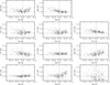 |
Fig. 23 Abundances for the 11 elements analysed by SPECIES with respect to iron, versus metallicity. This includes all the stars studied in Sect. 3.2.2, as well as from the GBS (Sect. 3.2.3). |
3.4 Offsets between different instruments
In order to use this code with spectra from different instruments, it is necessary to understand any offsets that are present between the parameters computed with spectra taken from different spectrographs. We compared the results we obtained for the stars used in the previous section, using four of the available instruments accepted by our code (HARPS, FEROS, UVES, and HIRES). The results of this comparison are shown in Fig. 24 for the atmospheric parameters and in Fig. 25 for the abundances. It is important to point out that not all the stars were observed with all instruments, therefore the number of stars compared per instrument varies, with 118 for FEROS, 115 for UVES, and 89 for HIRES.
We followed the same procedure used in the previous sections to analyse the significance of the differences in results. In this case, the comparison was done with respect to the HARPS results. The parameters for the Gaussian distributions adjusted to the difference in results are listed in Tables 9 and 10, for the atmospheric parameters and atomic abundance, respectively.
From both tables, it can be seen that all the quantities are in good agreement among all the instruments, with μ <1.5σ for each of them. This shows that SPECIES delivers consistent results with spectra from different high resolution spectrographs. We do want to mention that the only quantity with an offset larger than 1σ is seen in v sini, with respect to FEROS, with μ = 1.15 σ. We believe this is caused mainly because of the lower spectral resolution (R = 48 000) of FEROS, with respect to the rest of the instruments (R = 115 000, 110 000, and 67 000 for HARPS, UVES, and HIRES, respectively, as it appears in their documentation). This produces larger instrumental broadening, which, together with the macroturbulence contribution, dominate the absorption line profiles. In those cases, the rotational broadening has to be larger than ~2 km s−1 in order to make a contribution to the line profile that is measurable with FEROS (Murgas et al. 2013). This is also the reason behind the almost constant increase in difference for larger HARPS vsini, for low rotational velocities (up to 2 km s−1). For those low values, the line profiles measured with FEROS are still dominated by macroturbulence and instrumental broadening, resulting in a constant vsini for FEROS. This leads us to then set a minimum limit for the rotational velocity measured using FEROS spectra of 2 km s−1. For stars with slower rotation, the FEROS spectral resolution makes it difficult to obtain accurate results. In the future, we will perform the same comparison, but using spectra from the other instruments accepted by SPECIES that are not included in this analysis (i.e. Coralie, AAT).
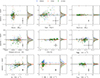 |
Fig. 24 Comparison between the stellar parameters obtained using spectra from different instruments, with respect to the ones obtained with HARPS. The y-axis for each plot corresponds to the difference between the parameters. Blue dots correspond to FEROS data, red triangles to UVES data, and green diamonds to HIRES data. For each panel, the right-hand plot corresponds to the distribution of the values, and solid line to the Gaussian distribution adjusted to each histogram. The black points in the bottom right of each plot represents the average uncertainty in the points. |
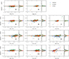 |
Fig. 25 Comparison between the abundances obtained with spectra from different instruments, with respect to the values obtained with HARPS spectra. The y-axis for each panel corresponds to the difference between the values from HARPS, and from FEROS (blue squares), UVES (red triangles), and HIRES (green diamonds). The right-hand plots show the distribution of the values, along with their Gaussian distribution fit. The black points in the bottom right of each plot represents the average uncertainty in the points. |
4 Summary and conclusions
In this paper we have presented a new code to derive stellar parameters in an automated way, using high resolution stellar spectra and minimal photometric inputs. The parameters calculated by SPECIES agree with previously published values at the 1σ level, for works using the same method as the one used in this work (EW measurements), as well as others (synthetic spectra). The code presented here computes all the stellar parameters in a self-consistent way, and we include in our values the rotational and macroturbulence velocity for each star, which is not present in most of the major catalogues that employ the EW method.
We also show the methods we used to derive the uncertainties for the atmospheric parameters, by providing analytic formulas that can be later used by others in the study of correlations between each parameter. We have listed the correlations present in our values, which can be linked to the physics that govern stars, or to the methods we use to derive them. We recommend the use of SPECIES for FGK dwarf and subgiant stars, for which we had tested it against a large sample of stars, and to use it with caution for giant stars, which will be tested more in future works. SPECIES has been used in Bluhm et al. (2016), Jones et al. (2018), Díaz et al. (2018), and Pantoja et al. (2018).
In future works we will apply the SPECIES code to accept spectra from more instruments, we will study a wide range of stars across a large evolutionary range to probe in detail the underlying nature of element production, and also we aim to include a module in SPECIES that will allow the calculation of precise parameters for M dwarf stars, where dust and molecules play a significant role.
Finally we note that SPECIES takes of the order of five minutes on a standard iMac desktop with a 3.2 Gb processor to obtain all the parameters for a single stellar spectrum. It can be run in single spectra mode or in parallel to simultaneously analyse large data sets.
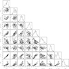 |
Fig. 26 Correlation between the atmospheric parameters, as well as the mass and age for each stars, derived by this code for HARPS spectra. The histograms the top of each column show the distribution of every single quantity. For log g, ξt, and age, the points farther than 3σ from the mean of the distribution were not included. |
Acknowledgements
MGS acknowledges support from CONICYT-PCHA/Doctorado Nacional/2014-21141037. JSJ acknowledges support by Fondecyt grant 1161218 and partial support by CATA-Basal (PB06, CONICYT). We acknowledge the very helpful comments from Y. V. Pavlenko and the anonymous referee. This research has made use of the VizieR catalogue access tool, CDS, Strasbourg, France. The original description of the VizieR service was published in Ochsenbein et al. (2000).
Appendix A Additional tables
Line data used in the computation of the atmospheric parameters.
Line data used in the computation of the atmospheric parameters.
Results from SPECIES for the GBS samples, for the stellar parameters.
Results from SPECIES for the GBS samples, for the chemical abundance of the elements in common with Jofré et al. (2015).
Appendix B Second method for the uncertainty in microturbulent velocity
As mentioned in Sect. 2.5.1, we include two different estimations for the uncertainty in the microturbulent velocity. The first one was already described (shown in the final catalogue as err_vt). Here we described the second method used (err_vt2). We used Eq. (12) from Magain (1984),
 (B.1)
(B.1)
where ξt is the microturbulent velocity, c = ∂A∕∂W change of abundance with equivalent width,  is the variance of the uncertainty of the equivalent widths (EWs),
  is the variance in the EWs, and SRW is the slope of the linear fit performed to EWs vs. Fe I abundance.
We assumed the same approximations than in Magain (1984), with one of them being that c = ci = ∂Ai∕∂Wi, the same for all the lines. In order to compute that value, we plotted ci vs Wi and found the ranges for which c is constant. We adopted c within that range to be the final value.
The dependency of ξt with SRW can be adjusted by the cubic spline from Eq. (3), with coefficients given by Eq. (4). The final value for the microturbulence velocity obtained by SPECIES is reached when SRW = 0 (Sect. 2.4), therefore in order to obtain (∂ξt∕∂SRW)|0 it is necessary to derive Eq. (3), and replace ξt by the SPECIES value in Eq. (4).
Finally,  and
and  are obtained from the ARES files for each star.
Appendix C Second method for the uncertainty in temperature
The method described here is very similar to the one used in Sect. 2.5.2, meaning that the uncertainty in the temperature is composed by two parts:
 (C.1)
(C.1)
where the first term corresponds to the contribution from the uncertainty in the microturbulence, and the second term is the contributionfrom the uncertainty in the slope of the dependence between the individual Fe I abundances and the excitation potential, χI. The first term is the same as the one derived in Sect. 2.5.2, but the second term is different and described here.
From Eq. (16.4) of Gray (2005), we can derive that:
 (C.2)
(C.2)
where log(w∕λ) is the reduced equivalent width of the line, logA = log(NE∕NH) the abundance of the element E to hydrogen, θex = 5040∕T, and χI is the excitation potential. If we assume that the equivalent width of the line will not change with respect to χI, but log A will, then when we differentiate with respect to χI, ∂∕∂χI, we obtain
 (C.3)
(C.3)
where  is the slope of the correlation between individual line abundances and excitation potential, and is one of the results obtained from the MOOG output file. The contribution from the uncertainty in the excitation potential will then be the above expression multiplied by the error in the slope.
Appendix D Catalogue description
The columns returned by SPECIES are as follow:
Col. 1: Star name.
Col. 2: Instrument used to obtain the spectra (HARPS, FEROS, HIRES, UVES, CORALIE, AAT).
Col. 3: Velocity in km s−1, obtained from the CCF (Sect. 2.2), used to correct the spectrum to the restframe.
Cols. 4–11: Atmospheric stellar parameters and their corresponding uncertainty (metallicity, temperature, surface gravity, and microturbulent velocity, respectively)
Cols. 12 and 13: Number of Fe I and Fe II lines used for the computation of the atmospheric parameters, respectively.
Col. 14: Exception to the atmospheric parameters. A value of one means the parameters were computed correctly. A value of two means that there were problems in the computation (parameters were repeated more than 200 times, or all of them were outside the permitted ranges), or that the code could not converge to a final value after performing over 1 million iterations.
Cols. 15–18: vsini and vmac for each star, with their respective uncertainties.
Cols. 19–54: Abundances for Na, Mg, Al, Si, Ca, Ti I, Ti II, Cr, Mn, Ni, Cu, and Zn, as well as their uncertainties (standard deviation from the mean) and the number of lines used.
Cols. 55–56: Individual abundances for Fe I and Fe II, respectively.
Cols. 57–64: Mass, age, loggiso (explained in Sect. 3.2.1), and radius obtained, along with their 54% and 16% confidence levels.
Col. 68: Tells whether the temperature computed from the method of Casagrande et al. (2010) was used as the final temperature or not, for the cases when no convergence was reached in the atmospheric parameters (Sect. 2.4).
Col 69: Tells whether the microturbulent velocity was set to 1.2 km s−1, for the cases when no convergence was reached in the atmospheric parameters (Sect. 2.4).
Col 70: Tells whether the surface gravity was set to be equal to loggiso (Sect. 2.6).
Cols. 71–72: Error in the microturbulence and temperature, computed using the methods described in Sects. B and C.
Cols. 73–75: Value, uncertainty, and relation used to obtain the temperature from photometry (Sect. 2.3.3).
Sample of the catalogue produced by our code.
References
- Adibekyan, V. Z., Sousa, S. G., Santos, N. C., et al. 2012, A&A, 545, A32 [NASA ADS] [CrossRef] [EDP Sciences] [Google Scholar]
- Arenou, F., Grenon, M., & Gomez, A. 1992, A&A, 258, 104 [NASA ADS] [Google Scholar]
- Asplund, M., Grevesse, N., Sauval, A. J., & Scott, P. 2009, ARA&A, 47, 481 [NASA ADS] [CrossRef] [Google Scholar]
- Beers, T. C., Flynn, C., Rossi, S., et al. 2007, ApJS, 168, 128 [NASA ADS] [CrossRef] [Google Scholar]
- Bensby, T., Feltzing, S., & Oey, M. S. 2014, A&A, 562, A71 [NASA ADS] [CrossRef] [EDP Sciences] [Google Scholar]
- Bessell, M. S. & Brett, J. M. 1988, PASP, 100, 1134 [NASA ADS] [CrossRef] [Google Scholar]
- Blackwell, D. E. & Lynas-Gray, A. E. 1994, A&A, 282, 899 [Google Scholar]
- Blanco-Cuaresma, S., Soubiran, C., Jofré, P., & Heiter, U. 2014, A&A, 566, A98 [NASA ADS] [CrossRef] [EDP Sciences] [Google Scholar]
- Bluhm, P., Jones, M. I., Vanzi, L., et al. 2016, A&A, 593, A133 [NASA ADS] [CrossRef] [EDP Sciences] [Google Scholar]
- Bond, J. C., Tinney, C. G., Butler, R. P., et al. 2006, MNRAS, 370, 163 [NASA ADS] [CrossRef] [EDP Sciences] [Google Scholar]
- Brewer, J. M., Fischer, D. A., Valenti, J. A., & Piskunov, N. 2016, ApJS, 225, 32 [NASA ADS] [CrossRef] [Google Scholar]
- Buchhave, L. A., Latham, D. W., Johansen, A., et al. 2012, Nature, 486, 375 [NASA ADS] [Google Scholar]
- Cardelli, J. A., Clayton, G. C., & Mathis, J. S. 1989, ApJ, 345, 245 [NASA ADS] [CrossRef] [Google Scholar]
- Carpenter, J. M. 2001, AJ, 121, 2851 [NASA ADS] [CrossRef] [Google Scholar]
- Casagrande, L., Portinari, L., & Flynn, C. 2006, MNRAS, 373, 13 [NASA ADS] [CrossRef] [Google Scholar]
- Casagrande, L., Ramírez, I., Meléndez, J., Bessell, M., & Asplund, M. 2010, A&A, 512, A54 [NASA ADS] [CrossRef] [EDP Sciences] [Google Scholar]
- Castelli, F. & Kurucz, R. L. 2004, IAU Symp., 210, Poster A20 [Google Scholar]
- Cutri, R. M., Skrutskie, M. F., van Dyk, S., et al. 2003, VizieR Online Data Catalog: II/246 [Google Scholar]
- Dekker, H., D’Odorico, S., Kaufer, A., Delabre, B., & Kotzlowski, H. 2000, in Optical and IR Telescope Instrumentation and Detectors, eds. M. Iye, & A. F. Moorwood, Proc. SPIE, 4008, 534 [Google Scholar]
- Demarque, P., Woo, J.-H., Kim, Y.-C., & Yi, S. K. 2004, ApJS, 155, 667 [NASA ADS] [CrossRef] [Google Scholar]
- Demircan, O. & Kahraman, G. 1991, Ap&SS, 181, 313 [NASA ADS] [CrossRef] [Google Scholar]
- Díaz, M. R., Jenkins, J. S., Tuomi, M., et al. 2018, AJ, 155, 126 [NASA ADS] [CrossRef] [Google Scholar]
- dos Santos, L. A., Meléndez,J., do Nascimento, J.-D., et al. 2016, A&A, 592, A156 [NASA ADS] [CrossRef] [EDP Sciences] [Google Scholar]
- Dotter, A. 2016, ApJS, 222, 8 [NASA ADS] [CrossRef] [Google Scholar]
- Ducati, J. R. 2002, VizieR Online Data Catalog: II/237 [Google Scholar]
- Edvardsson, B., Andersen, J., Gustafsson, B., et al. 1993, A&A, 275, 101 [NASA ADS] [Google Scholar]
- Feltzing, S. & Gustafsson, B. 1998, A&AS, 129, 237 [NASA ADS] [CrossRef] [EDP Sciences] [Google Scholar]
- Fischer, D. A. & Valenti, J. 2005, ApJ, 622, 1102 [NASA ADS] [CrossRef] [Google Scholar]
- Gaia Collaboration (Brown, A. G. A., et al. ) 2016, A&A, 595, A2 [NASA ADS] [CrossRef] [EDP Sciences] [Google Scholar]
- Gonzalez, G. & Vanture, A. D. 1998, A&A, 339, L29 [NASA ADS] [Google Scholar]
- González Hernández, J. I. & Bonifacio, P. 2009, A&A, 497, 497 [NASA ADS] [CrossRef] [EDP Sciences] [Google Scholar]
- Gray, D. F. 2005, The Observation and Analysis of Stellar Photospheres (Cambridge: Cambridge University Press) [CrossRef] [Google Scholar]
- Gustafsson, B., Bell, R. A., Eriksson, K., & Nordlund, A. 1975, A&A, 42, 407 [NASA ADS] [Google Scholar]
- Hauck, B. & Mermilliod, M. 1998, A&AS, 129, 431 [NASA ADS] [CrossRef] [EDP Sciences] [Google Scholar]
- Heiter, U., Jofré, P., Gustafsson, B., et al. 2015, A&A, 582, A49 [NASA ADS] [CrossRef] [EDP Sciences] [PubMed] [Google Scholar]
- Høg, E., Fabricius, C., Makarov, V. V., et al. 2000, A&A, 355, L27 [Google Scholar]
- Holmberg, J., Nordström, B., & Andersen, J. 2009, A&A, 501, 941 [NASA ADS] [CrossRef] [EDP Sciences] [Google Scholar]
- Ida, S. & Lin, D. N. C. 2004, ApJ, 616, 567 [NASA ADS] [CrossRef] [MathSciNet] [Google Scholar]
- Ida, S. & Lin, D. N. C. 2005, ApJ, 626, 1045 [NASA ADS] [CrossRef] [Google Scholar]
- Ivanyuk, O. M., Jenkins, J. S., Pavlenko, Y. V., Jones, H. R. A., & Pinfield, D. J. 2017, MNRAS, 468, 4151 [NASA ADS] [CrossRef] [Google Scholar]
- Jenkins, J. S., Jones, H. R. A., Pavlenko, Y., et al. 2008, A&A, 485, 571 [NASA ADS] [CrossRef] [EDP Sciences] [Google Scholar]
- Jenkins, J. S., Jones, H. R. A., Goździewski, K., et al. 2009, MNRAS, 398, 911 [NASA ADS] [CrossRef] [Google Scholar]
- Jenkins, J. S., Jones, H. R. A., Tuomi, M., et al. 2013, ApJ, 766, 67 [NASA ADS] [CrossRef] [Google Scholar]
- Jenkins, J. S., Jones, H. R. A., Tuomi, M., et al. 2017, MNRAS, 466, 443 [NASA ADS] [CrossRef] [Google Scholar]
- Jofré, P., Heiter, U., Soubiran, C., et al. 2014, A&A, 564, A133 [NASA ADS] [CrossRef] [EDP Sciences] [Google Scholar]
- Jofré, P., Heiter, U., Soubiran, C., et al. 2015, A&A, 582, A81 [NASA ADS] [CrossRef] [EDP Sciences] [Google Scholar]
- Jones, M. I., Jenkins, J. S., Brahm, R., et al. 2016, A&A, 590, A38 [NASA ADS] [CrossRef] [EDP Sciences] [Google Scholar]
- Jones, M. I., Brahm, R., Espinoza, N., et al. 2018, A&A, 613, A76 [CrossRef] [EDP Sciences] [Google Scholar]
- Kaufer, A., Stahl, O., Tubbesing, S., et al. 1999, The Messenger, 95, 8 [Google Scholar]
- Koen, C., Kilkenny, D., van Wyk, F., & Marang, F. 2010, MNRAS, 403, 1949 [Google Scholar]
- Kuiper, G. P. 1938, ApJ, 88, 472 [CrossRef] [Google Scholar]
- Kunitomo, M., Ikoma, M., Sato, B., Katsuta, Y., & Ida, S. 2011, ApJ, 737, 66 [NASA ADS] [CrossRef] [Google Scholar]
- Kupka, F., Piskunov, N., Ryabchikova, T. A., Stempels, H. C., & Weiss, W. W. 1999, A&AS, 138, 119 [NASA ADS] [CrossRef] [EDP Sciences] [MathSciNet] [PubMed] [Google Scholar]
- Magain, P. 1984, A&A, 134, 189 [NASA ADS] [Google Scholar]
- Mann, A. W., Feiden, G. A., Gaidos, E., Boyajian, T., & von Braun K. 2015, ApJ, 804, 64 [NASA ADS] [CrossRef] [Google Scholar]
- Martell, S. & Laughlin, G. 2002, ApJ, 577, L45 [NASA ADS] [CrossRef] [Google Scholar]
- Mayor, M., Pepe, F., Queloz, D., et al. 2003, The Messenger, 114, 20 [NASA ADS] [Google Scholar]
- Mordasini, C., Alibert, Y., Benz, W., Klahr, H., & Henning, T. 2012, A&A, 541, A97 [NASA ADS] [CrossRef] [EDP Sciences] [Google Scholar]
- Morton, T. D. 2015, Astrophysics Source Code Library [record ascl:1503.010] [Google Scholar]
- Murgas, F., Jenkins, J. S., Rojo, P., Jones, H. R. A., & Pinfield, D. J. 2013, A&A, 552, A27 [NASA ADS] [CrossRef] [EDP Sciences] [Google Scholar]
- Neves, V., Santos, N. C., Sousa, S. G., Correia, A. C. M., & Israelian, G. 2009, A&A, 497, 563 [NASA ADS] [CrossRef] [EDP Sciences] [Google Scholar]
- Ochsenbein, F., Bauer, P., & Marcout, J. 2000, A&AS, 143, 23 [NASA ADS] [CrossRef] [EDP Sciences] [Google Scholar]
- Pantoja, B. M., Jenkins, J. S., Girard, J. H., et al. 2018, MNRAS, in press [arXiv:1806.10067] [Google Scholar]
- Pavlenko, Y. V. 2017, Kinemat. Phys. Celest. Bodies, 33, 55 [NASA ADS] [CrossRef] [Google Scholar]
- Pavlenko, Y. V., Jenkins, J. S., Jones, H. R. A., Ivanyuk, O., & Pinfield, D. J. 2012, MNRAS, 422, 542 [NASA ADS] [CrossRef] [Google Scholar]
- Pecaut, M. J. & Mamajek, E. E. 2013, ApJS, 208, 9 [NASA ADS] [CrossRef] [Google Scholar]
- Piskunov, N. E., Kupka, F., Ryabchikova, T. A., Weiss, W. W., & Jeffery, C. S. 1995, A&AS, 112, 525 [NASA ADS] [Google Scholar]
- Queloz, D., Mayor, M., Weber, L., et al. 2000, A&A, 354, 99 [NASA ADS] [Google Scholar]
- Ryabchikova, T. A., Pakhomov, Y. V., & Piskunov, N. E. 2011, Kazan Izdatel Kazanskogo Universiteta, 153, 61 [NASA ADS] [Google Scholar]
- Santos, N. C., Israelian, G., & Mayor, M. 2000, A&A, 363, 228 [NASA ADS] [Google Scholar]
- Santos, N. C., Israelian, G., & Mayor, M. 2004, A&A, 415, 1153 [NASA ADS] [CrossRef] [EDP Sciences] [Google Scholar]
- Smith, R. C. 1995, Obs. Astrophys., 467 [Google Scholar]
- Sneden, C. A. 1973, Ph.D. Thesis, The University of Texas, Austin [Google Scholar]
- Sousa, S. G., Santos, N. C., Israelian, G., Mayor, M., & Monteiro, M. J. P. F. G. 2007, A&A, 469, 783 [NASA ADS] [CrossRef] [EDP Sciences] [Google Scholar]
- Sousa, S. G., Santos, N. C., Mayor, M., et al. 2008, A&A, 487, 373 [NASA ADS] [CrossRef] [EDP Sciences] [MathSciNet] [Google Scholar]
- Sousa, S. G., Santos, N. C., Adibekyan, V., Delgado-Mena, E., & Israelian, G. 2015, A&A, 577, A67 [NASA ADS] [CrossRef] [EDP Sciences] [Google Scholar]
- Strömgren, B. 1966, ARA&A, 4, 433 [NASA ADS] [CrossRef] [Google Scholar]
- Tinney, C. G., Butler, R. P., Marcy, G. W., et al. 2001, ApJ, 551, 507 [NASA ADS] [CrossRef] [Google Scholar]
- Tonry, J., & Davis, M. 1979, AJ, 84, 1511 [NASA ADS] [CrossRef] [Google Scholar]
- Torres, G., Fischer, D. A., Sozzetti, A., et al. 2012, ApJ, 757, 161 [NASA ADS] [CrossRef] [Google Scholar]
- Valenti, J. A., & Fischer, D. A. 2005, ApJS, 159, 141 [NASA ADS] [CrossRef] [MathSciNet] [Google Scholar]
- van Leeuwen F. 2007, A&A, 474, 653 [NASA ADS] [CrossRef] [EDP Sciences] [Google Scholar]
- Villaver, E. & Livio, M. 2009, ApJ, 705, L81 [NASA ADS] [CrossRef] [Google Scholar]
- Vogt, S. S., Allen, S. L., Bigelow, B. C., et al. 1994, in Instrumentation in Astronomy VIII, eds. D. L. Crawford, & E. R. Craine, Proc. SPIE, 2198, 362 [Google Scholar]
All Tables
Estimate of the uncertainties for the stellar parameters, separated in ranges of stellar temperature, for dwarf stars.
Mean of the Gaussian fits (in K) performed on the distribution of differences between the temperatures derived by SPECIES, and from using the colour relations from C10.
Mean of the Gaussian fits (in K) performed on the distribution of differences between the temperatures derived by SPECIES, and from using the colour relations from M15.
Mean of the Gaussian distribution (in K) adjusted to the histograms of the different between the temperature from SPECIES, and from interpolating between the models of P13.
Parameters of the Gaussian distributions adjusted to the difference of stellar parameters from SPECIES and from the literature.
Parameters of the Gaussian distributions adjusted to the difference of atomic abundance from SPECIES and from the literature.
Gaussian distribution parameters (μ, σ) obtained for the difference between stellar parameters from HARPS, and from other instruments.
Gaussian distribution parameters (μ, σ) obtained for the difference between atomic abundances from HARPS, and from other instruments.
Results from SPECIES for the GBS samples, for the chemical abundance of the elements in common with Jofré et al. (2015).
All Figures
|
Fig. 1 Flow diagram showing the process sequence of SPECIES. Each step is explained in Sect. 2. The green box represents the beginning of the diagram. |
| In the text | |
|
Fig. 2 Restframe correction applied to HD 10700. Top panel: Original spectra (grey), corrected spectra (black), and three reference lines at 6021.8, 6024.06, and 6027.06 Å (red). Bottom panel: Cross-correlation function (CCF) between the binary mask and the spectra. The red line corresponds to the Gaussian fit to the CCF, with a mean equal to −16.54 km s−1. |
| In the text | |
|
Fig. 3 Intrinsic JHK colours for dwarf (blue line) and giant (red line) stars, from Bessell & Brett (1988). The red point represents a star with H − K = 0.26 and J − H = 0.79. The distance between the point to the giant curve is 0.08 dex, and to the dwarf curve is 0.13 dex, therefore the star is classified as giant. The shaded area represents the H − K range for which the curves overlap, and no classification can be correctly performed. In those cases, the star is classified as dwarf. |
| In the text | |
|
Fig. 4 Photometric colours of main sequence stars, for different effective temperatures, from Pecaut & Mamajek (2013). Red lines represent the spline approximation for each curve. The temperature for a given colour is computed as the root of the (m1 − m2) − (m1,⋆ − m2,⋆) curve, wherem1 − m2 is the chosencolour, and m1,⋆, m2,⋆ are the star’s colours. |
| In the text | |
|
Fig. 5 logg vs. temperature for several stars in the literature. Red points represent giant stars, and blue points dwarf stars. The solid lines are the polynomials adjusted to each group, showed in Eq. (1). |
| In the text | |
|
Fig. 6 Top panel: ξt vs. SRW for a Solar spectrum. Bottom panel: fit of the spline coefficients as a function of microturbulence. |
| In the text | |
|
Fig. 7 Top panel: dependence of temperature with microturbulence (left) and SEP (right), for a Solar spectrum. Bottom panel: coefficients of the fit between T and ξt (left), and between T and SEP (right). |
| In the text | |
|
Fig. 8 Top panel: (left) dependence of metallicity with temperature for several values of microturbulence, (right) dependence of the coefficients a and b with ξt, so that [Fe/H] = a ⋅ T + b. Bottom panel: coefficients of the fit of [Fe/H] with T and ξt, so that a = m0 ⋅ ξt + m1 and b = m2 ⋅ ξt + m3. A vertical offset was applied to each coefficient for plotting purposes. |
| In the text | |
|
Fig. 9 Top panel: (left) dependence of surface gravity (logg) with individual Fe II abundance, (right) dependence of logg with temperature. Bottom panel: coefficients of the fits between logg with Fe II, and between logg with Teff, as shown in Eq. 12. A vertical offset was applied to each coefficient for plotting purposes. |
| In the text | |
|
Fig. 10 Results obtained for one of the solar spectrum used in SPECIES. First panel: log g –Teff space diagram. The red point represents the position of the Sun, with the final values obtained using our code (T = 5776 ± 73 K, [Fe/H] = 0.0± 0.1 dex, logg = 4.5 ± 0.2 cm s−2). Dotted lines represent the evolutionary tracks for stars with masses from 0.5 to 1.5 M⊙, and [Fe/H] = 0.0. The black line is the track for a 1.0 M⊙ star. Each point in the lines represent a different age. Remaining panels: distribution of the mass, age, and radius, for one of our HARPS solar spectra. The red dashed-solid-dashed lines represent the (16, 50, 84) quantiles, respectively. The results for this spectrum are listed in Table 3 as sun03. |
| In the text | |
|
Fig. 11 Top panel: histogram of the difference between logg and log giso. The blue line corresponds to the Gaussian distribution fit performed, with mean and sigma equal to μ = −0.004 and σ = 0.112, respectively. Bottom panel: difference between logg and log giso vs log g. Filled circlesare the stars laying within 2σ of the Gaussian fit performed to the histogram. Empty circles are the points laying beyond the 2σ level, for which the computation was performed a second time, but setting log g = log giso. |
| In the text | |
|
Fig. 12 Change of S versus abundance (left panels) and rotational velocity (middle panels), for each line of the solar spectra. The red lines represent the cubic spline fit performed over the data, and the vertical line shows the values where the minimum of S is reached. Right panels: line profiles, along with the final fit (red line) combining the instrumental profile, macroturbulence and rotational velocity. The horizontal black line around zero represents the residuals of the fit. |
| In the text | |
|
Fig. 13 Histograms of the difference between the temperature computed by SPECIES, and those using the colour relations from C10. The lines correspond to Gaussian distributions adjusted to the histograms, with mean values listed in Table 4. Each colour represents a different instrument: red for HARPS, blue for FEROS, green for HIRES, and orange for UVES. The different panels show the temperatures computed using different photometric colours, mentioned in Sect. 2. |
| In the text | |
|
Fig. 14 Histograms of the difference between the temperature computed by SPECIES, and by using the colour relations from M15. The lines correspond to the Gaussian fits for each distribution, and the colours represent the same instruments as in Fig. 13. The mean of the Gaussian fits are shown in Table 5. |
| In the text | |
|
Fig. 15 Histograms of the difference between the temperature computed by SPECIES, and those obtained by interpolating through the models of P13. The lines correspond to Gaussian distributions adjusted to the histograms, with mean values listed in Table 4. The mean of each Gaussian distribution is listed in Table 6. The colours represent the same instruments as in Fig. 13. |
| In the text | |
|
Fig. 16 Histograms of the difference between the metallicity (left panel), surface gravity (middle panel) obtained with SPECIES, and from using the photometric relations from Sects. 2.3.2 and 2.3.4 (right panel). The vertical lines correspond (from left to right) to the 16, 50 and 84 percentiles. |
| In the text | |
|
Fig. 17 Comparison between the values for different parameters obtained with our code and from literature. The y-axis in the plotscorrespond to the difference between both measurements, represented by different symbols and colours: blue circles to Sousa et al. (2008), red triangles to Brewer et al. (2016), green diamonds to Bond et al. (2006), orange squares to Bensby et al. (2014), and cyan stars to Ivanyuk et al. (2017). The black points in the bottom right of each plot represents the average uncertainty in the points. The histograms in the right panels of each of the plots show the distribution of the results, fitted by Gaussian functions, with parameters given in Table 7. |
| In the text | |
|
Fig. 18 Comparison between the surface gravity from SPECIES, and from the literature. In the top panel, the surface gravity from SPECIES corresponds to the results obtained from the convergence of the atmospheric parameters (Sect. 2.4), without the option of recomputing using log giso. In the bottom panel, the surface gravity from SPECIES corresponds to the log giso obtained forthe same stars (Sect. 2.6). |
| In the text | |
|
Fig. 19 Comparison between the abundances for different elements obtained with our code and from literature. The y-axis in the plotscorrespond to the difference between both measurements, represented by different symbols: blue circles to Sousa et al. (2008), red triangles to Brewer et al. (2016), green squares to Bond et al. (2006), orange squares to Bensby et al. (2014), and cyan stars to Ivanyuk et al. (2017). The black points in the bottom right of each plot represents the average uncertainty in the points. The histograms at the right panels of each plots show the distribution of the results, fitted by Gaussian functions. |
| In the text | |
|
Fig. 20 Results for the stellar parameters, obtained with SPECIES (x-axis), compared with what was found in the literature (y-axis), for the GBS sample. The different symbols denote different spectral types. The dashed line represents the 1:1 relation. |
| In the text | |
|
Fig. 21 Results for the chemical abundance of α and iron peak elements, obtained with SPECIES (x-axis), compared with what was found in the literature (y-axis), for the GBS sample. The different symbols denote different spectral types. The dashed line represents the 1:1 relation. |
| In the text | |
|
Fig. 22 Correlations between the stellar parameters computed by SPECIES. The red squares are the binned data points, and the blue lines correspond to the fits described in Eq. (16). The data used correspond to points within 3σ of their corresponding distribution. |
| In the text | |
|
Fig. 23 Abundances for the 11 elements analysed by SPECIES with respect to iron, versus metallicity. This includes all the stars studied in Sect. 3.2.2, as well as from the GBS (Sect. 3.2.3). |
| In the text | |
|
Fig. 24 Comparison between the stellar parameters obtained using spectra from different instruments, with respect to the ones obtained with HARPS. The y-axis for each plot corresponds to the difference between the parameters. Blue dots correspond to FEROS data, red triangles to UVES data, and green diamonds to HIRES data. For each panel, the right-hand plot corresponds to the distribution of the values, and solid line to the Gaussian distribution adjusted to each histogram. The black points in the bottom right of each plot represents the average uncertainty in the points. |
| In the text | |
|
Fig. 25 Comparison between the abundances obtained with spectra from different instruments, with respect to the values obtained with HARPS spectra. The y-axis for each panel corresponds to the difference between the values from HARPS, and from FEROS (blue squares), UVES (red triangles), and HIRES (green diamonds). The right-hand plots show the distribution of the values, along with their Gaussian distribution fit. The black points in the bottom right of each plot represents the average uncertainty in the points. |
| In the text | |
|
Fig. 26 Correlation between the atmospheric parameters, as well as the mass and age for each stars, derived by this code for HARPS spectra. The histograms the top of each column show the distribution of every single quantity. For log g, ξt, and age, the points farther than 3σ from the mean of the distribution were not included. |
| In the text | |
Current usage metrics show cumulative count of Article Views (full-text article views including HTML views, PDF and ePub downloads, according to the available data) and Abstracts Views on Vision4Press platform.
Data correspond to usage on the plateform after 2015. The current usage metrics is available 48-96 hours after online publication and is updated daily on week days.
Initial download of the metrics may take a while.