| Issue |
A&A
Volume 610, February 2018
|
|
|---|---|---|
| Article Number | A29 | |
| Number of page(s) | 11 | |
| Section | Stellar atmospheres | |
| DOI | https://doi.org/10.1051/0004-6361/201731530 | |
| Published online | 21 February 2018 | |
Tomography of cool giant and supergiant star atmospheres
I. Validation of the method
1
Institut d’Astronomie et d’Astrophysique, Université Libre de Bruxelles,
CP 226, Boulevard du Triomphe,
1050
Bruxelles, Belgium
e-mail: This email address is being protected from spambots. You need JavaScript enabled to view it.
2
Université Côte d’Azur, Observatoire de la Côte d’Azur, CNRS, Lagrange, CS 34229,
06304
Nice Cedex 4, France
3
Department of Physics and Astronomy at Uppsala University,
Regementsvägen 1, Box 516,
75120
Uppsala, Sweden
4
Laboratoire Univers et Particules de Montpellier, Université Montpellier II, CNRS,
34095
Montpellier Cedex 05, France
Received:
7
July
2017
Accepted:
22
November
2017
Abstract
Context. Cool giant and supergiant star atmospheres are characterized by complex velocity fields originating from convection and pulsation processes which are not fully understood yet. The velocity fields impact the formation of spectral lines, which thus contain information on the dynamics of stellar atmospheres.
Aim. The tomographic method allows to recover the distribution of the component of the velocity field projected on the line of sight at different optical depths in the stellar atmosphere. The computation of the contribution function to the line depression aims at correctly identifying the depth of formation of spectral lines in order to construct numerical masks probing spectral lines forming at different optical depths.
Methods. The tomographic method is applied to one-dimensional (1D) model atmospheres and to a realistic three-dimensional (3D) radiative hydrodynamics simulation performed with CO5BOLD in order to compare their spectral line formation depths and velocity fields.
Results. In 1D model atmospheres, each spectral line forms in a restricted range of optical depths. On the other hand, in 3D simulations, the line formation depths are spread in the atmosphere mainly because of temperature and density inhomogeneities. Comparison of cross-correlation function profiles obtained from 3D synthetic spectra with velocities from the 3D simulation shows that the tomographic method correctly recovers the distribution of the velocity component projected on the line of sight in the atmosphere.
Key words: stars: atmospheres / stars: AGB and post-AGB / supergiants / line: formation / radiative transfer / techniques: spectroscopic
© ESO 2018
1 Introduction
Cool giant and supergiant stars are evolved stars that play an important role in the chemical enrichment of the Galaxy. They have atmospheres with complex velocity fields, due to processes such as convection, pulsations, formation of molecules and dust, and the development of mass loss. These velocity fields impact the formation of spectral lines, the profiles of which become asymmetric, sometimes appearing double-peaked.
Schwarzschild (1952) suggested that the doubling of absorption lines originally observed in Cepheid variables is related to the passage of a shock wave through the photosphere. According to his scenario, in pulsating atmospheres (like those of long-period variable stars – LPVs – or Cepheids), when the shock front is located below the line-forming region, all lines are red-shiftedsince the matter in the line-forming region is falling down. When the shock front propagates through the line-forming region, the lines exhibit an additional blue-shifted component corresponding to rising matter. The intensity of the blue component increases with respect to the red component as the shock front reaches the upper layers of the stellar atmosphere. Finally, when the shock wave has passed through the entire photosphere, all lines exhibit only a blue-shifted component. This outward motion of the shock front was observed in Mira variables thanks to the tomographic method developed by Alvarez et al. (2000, 2001a,b), which was later applied to red supergiant star atmospheres by Josselin & Plez (2007; see Jorissen et al. 2016 for a recent review). The method allows one to recover the distribution of the component of the velocity field projected on the line of sight at different optical depths in the stellar atmosphere.
This paper describes a recent improvement of the tomographic technique which now resorts to the contribution function to access the depth of formation of the spectral line. Section 2 explains in detail the improved tomographic method and its comparison with the more basic approach proposed by Alvarez et al. (2001a). Section 3 deals with the comparison of line formation depths in 1D and 3D model atmospheres and demonstrates the reliability of the stellar velocity field reconstruction.
2 The tomographic method
The tomographic method requires three steps:
-
computation of 1D synthetic spectra of late-type giant or supergiant stars, and, from those, identification of the depth of formation of any given spectral line;
-
construction of numerical masks selecting lines forming in selected ranges of optical depths;
-
cross-correlation of these masks with series of spectra in order to extract information on the average shape of lines forming at a given depth in the atmosphere and thus on the corresponding velocity field (i.e., the Vz component of the velocity vector, where z is the axis in the cartesian frame of the star pointing towards the observer).
Each of these steps is now described in turn.
2.1 1D contribution function
The originalimplementation of the method (Alvarez et al. 2000, 2001a,b) was based on the Eddington-Barbier approximation to define the depth of line formation, stating thatthe emergent flux at wavelength λ is supposed to come from the layer located at the optical depth τλ = 2∕3. Thus, the line depression was assumed to form at that optical depth. However, Magain (1986) showed that the Eddington-Barbier approximation gives a valid depth of line formation only for sufficiently strong lines. In order to correctly assess the depth of line formation, the contribution function to the absolute line depression (CFLD) computed on a single ray (intensity) or disk-integrated (flux) has to be computed instead. This CFLD is different from the contributionfunction to the relative line depression derived by Magain (1986).
Following Magain (1986), Albrow & Cottrell (1996) derived the CFLD_SR (for a singleray) in the specific intensity, with Q ≡ Ic − Il:
 (1)
and in the flux by integrating on the disk (DI), considering a plane parallel atmosphere:
(1)
and in the flux by integrating on the disk (DI), considering a plane parallel atmosphere:
 (2)with
τ0 = ∫ κc,0 ρ dx: the continuum optical depth at a reference wavelength λ0 (ρ is the density). The τ0 scale can be adopteda s a proxy to the geometrical depth x;
κc,0: the continuum absorption coefficient at a reference wavelength λ0;
Ic: the continuous intensity;
Il: the line intensity;
κl: the line absorption coefficient;
Sl: the line source function;
τλ = ∫ κλρ dx: the optical depth along the ray (κλ is the total absorption coefficient at wavelength λ);
μ = cos θ: the cosine of the angle θ between the line of sight and the radial direction (μ = 1 for the direction towards the observer).
The optical depth τλ is related to the reference optical depth τ0 through
 (3)
(3)
2.2 Mask construction
All the necessary quantities for the CFLD computation have been extracted from the radiative-transfer code TURBOSPECTRUM (Plez 2012). The geometry of the 1D radiative transfer is explained in Gustafsson et al. (2008). The TURBOSPECTRUM code was previously modified by Lion et al. (2013) in order to include the computation of the CFLD. The radiative transfer was deliberately performed with zero microturbulence velocity (see Sect. 3.1).
The top panel of Fig. 1 displays the CFLDDI (computed with Eq. (2)) for a 1D MARCS model atmosphere with Teff = 3400 K and log g = −0.4 (1D-RSG model of Table 1). Its local maximum value (for a given wavelength λ) is a function of the reference optical depth τ0. The reference optical depth scale τ0 is computed at 5000 using only continuum opacities. The set of τ0 corresponding to the maximum CFLD for each wavelength defines a crest line. We call this crest line the “depth function” D(λ) (in the log τ0 scale, middle panel of Fig. 1); it specifies the optical depth τ0 at which the line(s) contributing at wavelength λ mainly form(s). The comparison of the depth function with a synthetic spectrum (bottom panel of Fig. 1) shows that, as expected, the cores of spectral lines form in outer layers while wings form in deeper layers.
Once the depth function is computed, the atmosphere is split into different slices (horizontal bands in the middle panel of Fig. 1) and spectral masks are constructed for each slice. Each mask is a collection of Dirac-like distributions. A set of eight tomographic masks were built. Each mask contains the positions of all lines whose depth function minimum falls within a limited range of optical depths. The optical depth full range is chosen as −4 .0 ≤ log τ0 ≤ 0 .0 with steps 0.5 in units of logarithmic optical depth. Following Alvarez et al. (2001a), only wavelengths where atomic lines dominate are kept in masks to achieve the best wavelength accuracy, which cannot always be reached with molecular lines.
Masks constructed in this way are then cross-correlated with either observed or synthetic stellar spectra. The resulting cross-correlation function (CCF) provides information about projected velocities (position of the minimum of the CCF), average strength (depth of the CCF) and shape of lines in a given atmospheric layer.
To test how well a given mask from the series of Fig. 1 probes lines formed in a given layer, the full width at half maximum (FWHM) of CFLD profiles (along the τ0 axis) of all lines contributing to the masks were computed. They are displayed in Fig. 2. The outermost mask C8 is not shown because its CFLD profiles are truncated due to the lack of extension of the 1D model atmosphere towards low optical depths (below log τ0 = −3.7), and the FWHM could not be computed. Figure 3 displays the average FWHM for each mask as a vertical line.It is seen that, with the chosen step of 0.5 in log τ0, neighboring masks have overlapping FWHM of their CFLD profiles. To probe the velocity field in non-overlapping layers, one may consider the set of masks {C1, C3, C5, C7} or {C2, C5, C7} (Fig. 3). However, this cross-talk between masks is moderate; indeed in Sect. 3.4 we will demonstrate that using all masks does allow us to reliably reconstruct the projected velocity field.
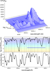 |
Fig. 1 Top panel: the CFLDDI for the 1D-RSG model (Table 1). Middle panel: the depth function D (λ) ≡ log τ0 (CFLDmax (λ)) corresponding to the crest line of the CFLD in the λ − log τ0 plane. Star symbols correspond to minima of the depth function. The horizontal bands represent the log τ0 ranges spanned by the different masks. The horizontal blue line identifies the spectral interval of the displayed CFLD (top panel). Bottom panel: the corresponding synthetic spectrum. |
Parameters of 1D MARCS model atmospheres and of the 3D simulation used in the present work.
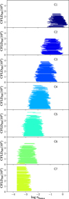 |
Fig. 2 FWHM of the CFLDDI for lines contributing to spectral masks C1–C7 (C8 not represented, see text) computed from the 1D-RSG model of Table 1. The color-code identifies the masks as in the middle panel of Fig. 1. |
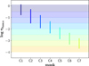 |
Fig. 3 Vertical lines: average FWHM of the CF of lines contributing to spectral masks C1–C7 (C8 not represented,see text) computed from the 1D-RSG model of Table 1. Horizontal bands: optical depth ranges used for selecting lines in a given mask. The color code has no spectral meaning. |
2.3 Comparison of “old” and “new” tomographic techniques: the Mira variable V Tau
To test the tomographic method based on the CFLD, we first tried to reproduce the results obtained by Alvarez et al. (2001a) for the Mira variable star V Tau.
For this purpose, another set of spectral masks was constructed with the same hypotheses as in Alvarez et al. (2001a), except for the Eddington-Barbier condition replaced by the following: the core of a given spectral line is forming in the layer where the depth function (i.e., the maximum of the CFLD, computed with Eq. (2), along the wavelength axis) reaches the lowest optical depth (identified by star symbols in the middle panel of Fig. 1). The construction of the spectral masks proceeds as in Alvarez et al. (2001a):
-
A 1D MARCS model atmosphere is used with Teff = 3500 K and log g = 0.9 (1D-AGB model of Table 1). It must be mentioned that the model atmosphere used by Alvarez et al. (2001a) was computed with the Plez et al. (1992) version of the MARCS code whereas the model used here is from the more recent MARCS grid (Gustafsson et al. 2008).
-
Linelists are used containing data for the same atoms and molecules, and identical CNO abundances and isotopic ratios.
-
A reference optical depth scale at 1.2 μm is adopted.
-
The atmosphere is divided into eight layers in the range
 with step 0.75 in units of logarithmic optical depth.
 -
The masks-only wavelengths corresponding to atomic lines are kept.
Figure 4 shows the number of lines in the various masks together with the distribution of lines in masks from Alvarez et al. (2001a); it illustrates the fact that our MARCS model atmosphere does not extend as far as the model used by Alvarez et al. (2001a). Therefore, all lines which form in the optical depth range 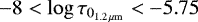 (masks C6–C8) in Alvarez et al. (2001a) are merged in our mask C5.
The obtained masks were cross-correlated with an ELODIE (Baranne et al. 1996) spectrum of V Tau. Figure 5 compares the resulting CCFs to those of Alvarez et al. (2001a). The discrepancy between CCFs in the outermost mask C5 is due to different extensions of the model atmospheres described above. Our CCFs show very good agreement with those obtained by Alvarez et al. (2001a). The comparison with our more sophisticated method based on the CFLD indicates that the approach of Alvarez et al. (2001a) (using the Eddington-Barbier condition) yields meaningful results. It was indeed able to reveal the occurrence of the Schwarzschild scenario in Mira variables.
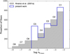 |
Fig. 4 Distribution of lines in spectral masks C1–C8 obtained by Alvarez et al. (2001a; gray shaded histogram) and in the present work (blue line) for the 1D-AGB model (Table 1). |
2.4 Mean formation depth of spectral lines
Instead of constructing masks from the maximum of the CFLD, one may use the average depth of line formation obtained by the first moment of the CFLD. For any given wavelength, Magain (1986) defines (his Eq. (22), also used in Amarsi 2015):
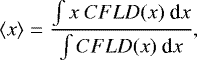 (4)
with x = log τ0, that is the logarithmic reference optical depth.
(4)
with x = log τ0, that is the logarithmic reference optical depth.
A set of five masks was constructed as in Sect. 2.3, and the log τ0 corresponding to the maximum of the CFLD was replaced by the average line formation depth computed with Eq. (4). The resulting masks were then cross-correlated with the observed spectrum of V Tau. The resulting CCFs are shown in Fig. 5 (green line) together with those obtained in Sect. 2.3 from the maxima of the CFLD. They are characterized by noisy and less contrasted profiles in masks C1–C3.
Actually, the depth of line formation, as derived either from the extrema of the CFLD or from a weighted average, will differ in the case of skewed CFLDs, as is mostly the case for weak lines forming deep in the atmosphere. Because of skewed CFLD, the averaging method (Eq. (4)) will attribute to weak lines a formation depth higher up in the atmosphere. Thus, they will be included in masks also containg stronger lines often characterized by more symmetric CFLDs and forming naturally higher up in the atmosphere. As a result, the inner masks will contain fewer lines and give rise to noisy and less contrasted CCFs.
Thus, we adopted the approach based on the maximum of the CFLD (the so-called depth function) which also provides results that are more consistent with Alvarez et al. (2001a).
 |
Fig. 5 Black dashed line: sequence of CCFs obtained from a V Tau spectrum (JD 2451093.5) using masks of Alvarez et al. (2001a; their Fig. 18). Red line: the CCF profiles obtained from the same spectrum using masks with identical log τ limits but built using maxima of the CFLD, as described in Sect. 2.2. Green line: CCF profiles obtained from the same spectrum using masks built from Eq. (4) in Sect. 2.4. |
3 Application to 3D atmospheres of red supergiants
The tomographic method uses 1D model atmospheres for mask construction. However, in real stars like Mira and supergiant stars, multi-dimensional dynamical processes occur, and Chiavassa et al. (2011) showed that more than one hydrostatic 1D model is necessary to reproduce the thermodynamical structure of the radiative hydrodynamics (RHD) simulation. In such complex atmospheres, the depths of formation of spectral lines will likely differ from the 1D prediction.
In order to assess the reliability of the tomographic method in 3D dynamical atmospheres, it was tested on snapshots from numerical 3D RHD simulations performed with the CO5BOLD code (Freytag et al. 2012). The 3D simulations are characterized by realistic input physics and reproduce the effects of convection and non-radial waves (Chiavassa et al. 2011). The parameters of the 3D simulation used in the analysis are presented in Table 1.
The 3D pure-LTE radiative transfer code Optim3D (Chiavassa et al. 2009) was used to compute synthetic spectra and intensity maps from a snapshot of the 3D simulations (Fig. 6). The code takes into account the Doppler shifts caused by the convective motions. The radiative transfer is calculated using pre-tabulated extinction coefficients generated with the MARCS code (Gustafsson et al. 2008). These tables are functions of temperature, density, and wavelength, and are computed by adopting the solar composition of Asplund et al. (2006). They include the same extensive atomic and molecular data as the MARCS models usedin the present work.
The computation of the CFLD was implemented in the OPTIM3D code. The 3D CFLDSR and 3D CFLDDI are described in Sects. 3.1 and 3.2, respectively.
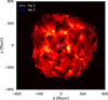 |
Fig. 6 Intensity map at λ = 4040.07 Å for a snapshot of the 3D simulation. The intensity range is [0; 250] |
3.1 The CFLD for the 3D simulation: single ray
If we consider a single ray of the 3D simulation, the 3D CFLDSR is computedusing Eq. (1) for the direction towards the observer, that is with μ = 1.
Figure 7 displays the temperature, Vz, and 3D CFLDSR structures for a representative slice through the 3D numerical box. The 3D CFLDSR was computed at λ = 4040.07 Å (corresponding to an Ir I atomic line). The Ir I line was selected arbitrarily and contributes to the C1 mask computed in Sect. 2.2. Figure 7 demonstrates the complexity of a 3D atmosphere with respect to a 1D atmosphere. Here, the velocity field is not homogeneous but is characterized by multiple shocks which affect the temperature structure and the 3D CFLD. Thus, the CFLD in the 3D atmosphere is not smooth like in 1D.
A more detailed study of the 3D CFLDSR is performed for a single ray of the 3D numerical box (ray 1 in Fig. 6). The velocities of the 3D simulation were set to zero in the Optim3D code to have a direct comparison with hydrostatic 1D calculations (also in Sects. 3.2 and 3.3). The extinction coefficients used in Optim3D were constructed with no micro-turbulent broadening. The same approach was applied in the 1D radiative transfer computation where the microturbulence was set to zero in order to compare the CFLDs without any fudge parameter which mimics the velocity field at small scales. Thus, the velocity information will emerge only from the 3D simulation itself (see Sect. 3.4). The continuum optical depth scale at 5000 was taken as a reference scale. The 3D CFLDSR is shown in Fig. 8. It has a more complicated structure than the 1D CFLDDI (top panel of Fig. 1). The 3D CFLDSR shows multiple maxima at a given wavelength, which means that a given spectral line forms at several depths in the atmosphere.
The top panel of Fig. 9 displays the 3D CFLDSR as a function of τ0 at λ = 4040.07 for two single rays of the 3D simulation and for the corresponding 1D MARCS model atmosphere (i.e., 1D-RSG model of Table 1). The rays were selected close to the center of the stellar disk and correspond to dark and bright areas on the surface (rays 1 and 2 in Fig. 6, respectively). The location of rays has an impact on the height of the 3D CFLD profile. The temperatures probed by the ray in a dark region (ray 1; green line in Fig. 9) are generally cooler than those probed by the ray located in a bright region (ray 2; orange line in Fig. 9). Thus, its continuum intensity (used in Eq. (1) and displayed in the second panel of Fig. 9) and the CFLD are also lower. Figure 9 also compares the temperature (fifth panel), density (sixth panel) and Vz velocity (seventh panel) for single rays of the 3D simulation and for the corresponding 1D model atmosphere.
The 1D model is characterized by a monotonic and continuous growth of the temperature and density towards the stellar interior. On the contrary, the corresponding 3D profiles show non-monotonous temperature and density variations, including shocks, and complex velocity variations. The presence of a shock is indicated by a strong negative gradient in the velocity  (see the bottom panel of Fig. 9), that signals compression of outward moving (Vz < 0) gas. The corresponding atmospheric layers are characterized by temperature and density discontinuities.
The temperature and density inhomogeneities affect the line source function and opacity (third and fourth panels of Fig. 9). These terms together with the continuum intensity contribute to Eq. (1). This explains the splitting of the line formation depths seen in Fig. 8, and not seen in the 1D CFLD.
Chiavassa et al. (2009) showed that for some rays of the 3D simulation, the optical depth scale may vary by a large amount between two neighbor grid points (e.g., from τ = 1 to a few hundred). The intensity is poorly estimated along those few rays. We tried to overcome this problem by interpolating the intensity, but without reliable results. Fortunately, the intensity only impacts the height of the 3D CFLD but does not affect the location of its maximum along the optical depth scale. Thus, the comparison with the 1D CFLD is not affected by the poor grid resolution of 3D simulations at large depths.
Figure 9 shows that the temperature and density structures are obviously not similar along different single rays of the 3D simulation, and differ as well from those of a 1D model atmosphere. All rays of the 3D numerical box have to be taken into account, and the 3D CFLDDI has to be computed, as we do in the following section.
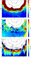 |
Fig. 7 Temperature T, projected velocity Vz and log CFLDSR structures for the slice through the 3D numerical box. The observer is at the bottom of each figure. Black contour lines on all panels show the thermal stratification. |
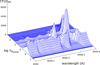 |
Fig. 8 3D CFLDSR for a single ray of the 3D simulation (ray 1 on Fig. 6) in the same spectral range as the 1D CFLDDI in the top panel of Fig. 1. A spectral resolution of R = 900 000 was adoptedfor plotting purposes. |
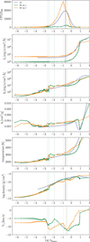 |
Fig. 9 CFLDSR, continuum intensity Ic, line source function Sl, line absorption coefficient kl , temperature, logarithmic density and Vz structures at λ = 4040.07 for two single rays of the 3D snapshot located in bright and dark areas on the stellar disk (orange and green colors indicate rays 2 and 1, respectively, in Fig. 6) and for the corresponding 1D-RSG model of Table 1 (blue dashed line). Vertical lines correspond to local maxima of CFLDs. |
3.2 The CFLD for the 3D simulation: stellar disk
For the whole stellar disc, the derivation of the 3D CFLDDI cannot be performed with Eq. (2), which describes a plane-parallel atmosphere.
Following Albrow & Cottrell (1996) and Amarsi (2015), we define the absolute depression in the line intensity as
 (5)
where the z index means that the intensity is considered along the z axis (pointing towards the observer). In the above relation, all quantities depend on wavelength λ, and optical depth τ, which is itself a function of the considered point in the atmosphere: τ = τ(x, y, z); it is computed from
(5)
where the z index means that the intensity is considered along the z axis (pointing towards the observer). In the above relation, all quantities depend on wavelength λ, and optical depth τ, which is itself a function of the considered point in the atmosphere: τ = τ(x, y, z); it is computed from  where zs is the z coordinate at the surface.
The absolute line depression in the flux is then
 (6)
where
(6)
where
-
Fc and Fl are continuum and line fluxes respectively;
-
Q(x, y, zs) is computed at the surface;
-
R is the stellar radius.
Since no flux is coming from the opposite side of the star, the integration in Eq. (6) is performed over a hemisphere.
Since Q obeys a transfer equation (e.g., Eq. (7) of Albrow & Cottrell 1996), its formal solution at the surface may be written:
 (7)
with z being an implicit function of τ as defined above, and with
(7)
with z being an implicit function of τ as defined above, and with
 (8)
(8)
We note that Eqs. (6) and (7) are equivalent to Eq. (11) of Amarsi (2015). As compared to Albrow & Cottrell (1996) formalism, there is no need for the variable μ in our treatment (μ ≡ 1 because all rays are parallel and in the direction of the observer).
Substituting Q in the definition of U then leads to
 (9)
(9)
The contribution function to the line depression in the flux is therefore:
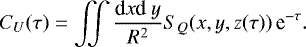 (10)
(10)
Despite the fact that this function is applicable to a 3D model, it is nevertheless a function of the single variable τ.
The link between τ and the geometrical depth z is however different for each of the considered parallel rays, described by the variables x, y. This is illustrated in Fig. 10 and is caused by the dynamics that affects the opacity and structure of the atmosphere from ray to ray. For convenience, this diversity in the relationship between τ and z depending on (x, y) is illustrated by showing the spread in the run of τ with radial distance  within the star for a few (x, y) pairs (represented by the ray number i, j).
Equation (10) may be discretized as follows:
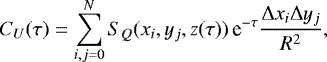 (11)
and a reference τ0 scale may be defined (Eq. (3)), so that
(11)
and a reference τ0 scale may be defined (Eq. (3)), so that
 (12)
(12)
and
 (13)
(13)
![Mathematical equation: \begin{equation} -S_{{\rm l},z} \Big(x_i,y_j,z(\tau_0)\Big)\bigg] {\rm e}^{-\tau } \frac{ \mathrm{\Delta} x_i \mathrm{\Delta} y_j}{R^2} \label{Eq: finalCU}, \end{equation}](/articles/aa/full_html/2018/02/aa31530-17/aa31530-17-eq20.png) (14)
where N is the number of grid points in the numerical box along the z axis. Since the numerical grid is equidistant, Δxi = Δyj. In the above relation, all quantities depend moreover on λ.
(14)
where N is the number of grid points in the numerical box along the z axis. Since the numerical grid is equidistant, Δxi = Δyj. In the above relation, all quantities depend moreover on λ.
We note that CU(τ0) fulfills the usual requirements for a contribution function, namely: CU (τ0)≠0 only if κl ≠0 and Sl≠Ic, and CU(τ0) > 0 if Sl < Ic (absorbing region). In principle, the stellar radius needs to be computed to use Eq. (14); however, it acts as a normalization constant. Following the method explained in Chiavassa et al. (2011), the temperature and luminosity were averaged over spherical shells, and the stellar radius was computed using Eq. (5) from Chiavassa et al. (2011). It amounts to 582 ± 5 R⊙ for the 3D simulation from Table 1.
The 3D CFLDDI was computed for the whole stellar disk using Eq. (14). We note that rays located in regions of the numerical box where the column density is so low that the integrated optical depth falls below the limit of τ = 2∕3 were not considered. The resulting 3D CFLDDI is displayed in Fig. 11 in the same spectral interval as the 3D CFLDSR for the central ray of the 3D simulation (ray 1, see Fig. 8) and the 1D CFLDDI (see top panel of Fig. 1). The 3D CFLDDI profiles are characterized by a single maximum in the log τ0 - CFLD plane, similar to the 1D CFLD behavior.
The top panel of Fig. 12 compares the 3D CFLDDI at λ = 4040.07 with the corresponding 1D CFLDDI (computed using Eq. (2)). A single-peaked 3D CFLDDI is the result of a monotonic behavior of the average temperature profile of the 3D numerical box (see bottom panel of Fig. 12). Since many rays of the 3D simulation are taken into account, the atmospheric inhomogeneities largely average out, so that the global disk produces a 3D CFLD resembling a 1D one.
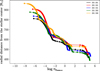 |
Fig. 10 Relation between the reference τ0 scaleand radial distances (in R⊙) from points along five rays of the 3D simulation to the stellar center. Numbers on the labels correspond to i and j indices of selected rays. |
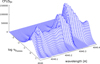 |
Fig. 11 3D CFLDDI for the whole stellar disk, to be compared with top panel of Fig. 1. A spectral resolution of R = 900 000 was adoptedfor plotting purposes. |
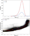 |
Fig. 12 Top panel: CFLDDI for the whole stellar disk (red line) and for the 1D-RSG model of Table 1 (blue line) computed at λ = 4040.07. Bottom panel: thermal structures for all rays contributing to the stellar disk. Darker areas correspond to more frequent temperature values. The red line is the average 3D thermal profile. The orange dashed lines show the 1σ values around the average. The blue line is the 1D-RSG model thermal profile. |
3.3 Tomographic masks
This section aims at validating the fact that tomographic masks computed from a 1D static model atmosphere do not lose their discriminating properties in a dynamical atmosphere. In other words, we need to check that a set of lines that originate from the same given depth in a static atmosphere (thus defining a mask) continue to form in the same layers in a dynamical atmosphere. Of course, these layers will not necessarily be at the same depth in the dynamical atmosphere, and multiple layers may contribute to a given line (because the run of the temperature is no longer monotonic). But the key property to be satisfied is that all lines defining a given mask from a 1D static atmosphere behave similarly in a dynamical atmosphere. Moreover, we need to define the masks from a static atmosphere to be able to subsequently reveal complex matter motions in a dynamical atmosphere (showing up as multiple peaks in the 3D CFLD and corresponding CCFs).
In order to compare the line formation depths between the 1D model atmosphere and the 3D simulation, the set of eight tomographic masks constructed in Sect. 2.2 from a 1D RSG model atmosphere (Table 1) were used. The distribution of the number of lines in masks is shown in the right panel of Fig. 13. The optical depths corresponding to maxima of the 3D CFLDDI in a log τ0 − CFLD plane for all lines contributing to a given mask were extracted and displayed as histograms on the left panel of Fig. 13. Red-colored areas indicate regions probed by masks according to the 1D model atmosphere.
The histograms in Fig. 13 move along the optical depth axis from the deepest layers (C1) to the outermost (C8) in the same manner as 1D line formation depths. The important conclusion at this point is that the line formation depths in the 3D model stay within the range expected from the 1D model and do not get scattered all over the τ0 scale for any given mask. Thus, masks constructed from a 1D model keep their power to probe different atmospheric depths in a dynamic atmosphere of the kind we used here. Mask C8 is characterized by a shift of line formation depths towards lower optical depths (outer layers). It is related with the fact that the 3D model atmosphere is more extended than the 1D model atmosphere. This is due to the turbulent pressure naturally included in 3D simulations that lowers the effective gravity and consequently stretches the atmosphere (Gustafsson & Plez 1992; Gustafsson et al. 2008; Chiavassa et al. 2011).
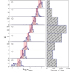 |
Fig. 13 Properties of masks C1–C8 computed from the 1D-RSG model (Table 1). Left panel: the distribution of formation depths of lines contributing to tomographic masks C1–C8 for the whole stellar disk (blue histograms). Red bands represent the optical depth ranges used for selecting lines in a given mask from the 1D CFLD. Right panel: the distribution of the number of lines in spectral masks C1–C8. |
3.4 Can tomography reliably recover the Vz distribution in a 3D atmosphere?
3.4.1 Single ray
Previous sections showed that the line formation process in a 3D atmosphere is more complex than in a 1D model atmosphere (as seen in Figs. 7 and 9) leading to a small but real spread of line-forming regions in the atmosphere. This means that a given line will contribute to the CCF of its corresponding mask with different velocities. The resulting CCF will have multiple peaks which are the signature of the presence of a velocity field in the atmosphere. This section aims at confirming that the peaks in the CCF are representative of the velocities. For this purpose, the 3D simulation is of invaluable help since the velocity value at each grid point of the numerical box is obviously known.
For this analysis, a single ray of the 3D numerical box (ray 1) was chosen, and a synthetic spectrum was computed with a spectral resolution R = λ∕Δλ = 200 000, including and not including the velocity field in the 3D simulation. Then, it was cross-correlated with the tomographic mask C6 obtained in Sect. 2.2. The right panel of Fig. 14 displays the resulting cross-correlation profile with and without the velocity field. The CCF has three components, at −6, −9 and −12 km s−1. The CCF produced with all velocities at zero is useful to measure thelevel of correlation noise (caused by the forest of neighboring lines).
As a next step, the optical depths corresponding to all maxima of the 3D CFLDSR for all wavelengths contributing to the mask C6 were retrieved. They are displayed as histograms on the middle panel of Fig. 14 weighted (b) and not weighted (a) by the respective CFLDSR value. Weighting of the histogram by the CFLD shows which peaks on the CFLD significantly contribute to the resulting intensity used for the CCF computation.
Then, the Vz velocities along a given ray (left panel of Fig. 14) attributed to the optical depth ranges from the middle panel of Fig. 14 were extracted. They are displayed ashistograms (green color) in the right panel of Fig. 14 with the binning step equal to 1.5 km s−1 to match the resolution of the CCF. The histograms have peaks at −6, −9 and −12 km s−1 which are present on the CCF. This shows that our method correctly recovers the velocity value of all components on the CCF.
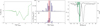 |
Fig. 14 Left panel: Vz as a function of the reference optical depth for the ray 1 of the 3D simulation. Middle panel: distribution of formation depths of lines contributing to the mask C6 for the ray 1 weighted (b) and not weighted (a) by the CFLD. Right panel: CCF obtained by cross-correlation of the synthetic spectrum [with (black solid line) and without (black dashed line) including the velocity field in the 3D simulation] for the ray 1 of the 3D snapshot with the mask C6. Green bars show the distribution of velocities corresponding to formation depths of lines contributing to the mask C6. |
3.4.2 Integrated flux
The same analysis was performed for the whole 3D simulation. Figure 15 shows the CCFs and the velocity histograms computed in the same way as those for a single ray described above. Here, the CCFs in the innermost masks C1–C2 have a main peak at 2 km s−1. In mask C3, a blue-shifted component is clearly visible at −8 km s−1. Moving to outermost mask C8, the strength of the blue-shifted peak increases, while that of the red-shifted peak decreases and shifts to 5 km s−1. The evolution of peaks on the CCFs from red-shifted to blue-shifted while probing more and more external layers does not follow the Schwarzschild scenario, which describes the global envelope pulsation in Mira variables. In supergiant stars instead, the tomographic method probes local motions involving specific rays.
In order to quantify the agreement between the velocity distributions and the CCFs, we first measured the velocity range they cover in each mask. In order to determine that velocity range for CCFs, we assume that the level of the correlation noise does not exceed 10% of the total contrast of a given CCF. The velocity spread is displayed in the top panel of Fig. 16 and is roughly similar for the CCFs and the histograms. Therefore, the CCFs correctly reproduce the range of velocities of the atmosphere. As a next step, the FWHM of velocity distributions and CCF profiles were computed. They are shown on the bottom panel of Fig. 16. Despite a slight difference in the FWHM of the CCFs and the histograms (especially for masks C3, C4, C6, and C7), we may nevertheless consider that the tomographic method is able to correctly recover the Vz distribution.
The top panel of Fig. 17 displays the CCFs for each spectral mask as a function of the log τ0 range and the velocity. The comparison with the distribution of velocities of the 3D simulation (the bottom panel of Fig. 17) shows that CCFs recover well the distribution of velocities.
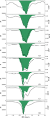 |
Fig. 15 Sequence of CCF profiles (black solid line) obtained by cross-correlation of a synthetic spectrum (with included velocity field) for the whole stellar disk with tomographic masks C1–C8. Green bars show the distribution of velocities corresponding to all formation depths of lines contributing to masks C1–C8. |
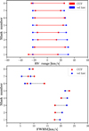 |
Fig. 16 Top panel: velocity range covered by CCFs (red color) and velocity histograms (blue color) from Fig. 15 in each spectral mask. Bottom panel: FWHM of CCF profiles (red color) and velocity distributions (blue color) for all masks. In masks C6 and C7 the FWHM were measured separately for each of the two peaks. The dashed black line connects the FWHM values of corresponding peaks. |
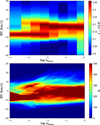 |
Fig. 17 Top panel: CCFs computed on a snapshot spectrum from the 3D simulation as a function of the reference optical depth scale and the velocity. The color code shows the minimum (red color) and maximum (blue color) values of each CCF. Bottom panel: distribution of Vz velocities of the 3D simulation as a function of the reference optical depth. The color code shows areas with high (red) or low (blue) density of points. |
4 Conclusions
The present paper applies tomography to red supergiant atmospheres, aiming at recovering the projected velocity field at different optical depths in the stellar atmosphere. Our implementation of tomography includes the computation of the contribution function to the line depression to correctly assess the formation depth of spectral lines. The method was compared to a simpler procedure proposed by Alvarez et al. (2001a). We reproduce these earlier results for the Mira variable V Tau, thus validating all the conclusions from this earlier study.
The tomography was applied to 3D RHD simulations in order to check whether the Vz velocity fields in their atmospheres could be recovered by the method. For this purpose, the CFLD was calculated for individual rays of the 3D simulation and for the whole stellar disk. It showed that in 3D simulations the spectral lines do not form in a restricted range of reference optical depths as in 1D model atmospheres. The line formation is spread over different optical depths due to convection present in 3D simulations.
By comparing the CCF computed from the synthetic spectra originating from 3D simulations with the velocity distribution (available from the very same simulations), it was shown that the CCFs indeed nicely trace the projected velocity fields in the atmosphere.
The application of the tomographic method to observed spectra of actual red supergiant stars is deferred to a forthcoming paper.
Acknowledgments
K.K. acknowledges the support of a FRIA (FNRS) fellowship. S.V.E. is supported by a grant from the Fondation ULB. This work was granted access to the HPC resources of “Observatoire de la Côte d’Azur - Mésocentre SIGAMM”. We wish to thank the referee Amish Amarsi for helpful comments which contributed to an improvement of the paper.
References
- Albrow, M. D., & Cottrell, P. L. 1996, MNRAS, 278, 337 [NASA ADS] [Google Scholar]
- Alvarez, R., Jorissen, A., Plez, B., Gillet, D., & Fokin, A. 2000, A&A, 362, 655 [NASA ADS] [Google Scholar]
- Alvarez, R., Jorissen, A., Plez, B., et al. 2001a, A&A, 379, 288 [NASA ADS] [CrossRef] [EDP Sciences] [Google Scholar]
- Alvarez, R., Jorissen, A., Plez, B., et al. 2001b, A&A, 379, 305 [NASA ADS] [CrossRef] [EDP Sciences] [Google Scholar]
- Amarsi, A. M. 2015, MNRAS, 452, 1612 [NASA ADS] [CrossRef] [Google Scholar]
- Asplund, M., Grevesse, N., & Jacques Sauval, A. 2006, Nucl. Phys. A, 777, 1 [NASA ADS] [CrossRef] [Google Scholar]
- Baranne, A., Queloz, D., Mayor, M., et al. 1996, A&AS, 119, 373 [NASA ADS] [CrossRef] [EDP Sciences] [Google Scholar]
- Chiavassa, A., Plez, B., Josselin, E., & Freytag, B. 2009, A&A, 506, 1351 [NASA ADS] [CrossRef] [EDP Sciences] [MathSciNet] [Google Scholar]
- Chiavassa, A., Freytag, B., Masseron, T., & Plez, B. 2011, A&A, 535, A22 [NASA ADS] [CrossRef] [EDP Sciences] [Google Scholar]
- Freytag, B., Steffen, M., Ludwig, H.-G., et al. 2012, J. Comput. Phys., 231, 919 [Google Scholar]
- Gustafsson, B., & Plez, B. 1992, in Instabilities in Evolved Super- and Hypergiants, eds. C. de Jager & H. Nieuwenhuijzen (Amsterdam: North-Holland), 86 [Google Scholar]
- Gustafsson, B., Edvardsson, B., Eriksson, K., et al. 2008, A&A, 486, 951 [NASA ADS] [CrossRef] [EDP Sciences] [Google Scholar]
- Jorissen, A., Van Eck, S., & Kravchenko, K. 2016, in Astrophysics and Space Science Library, eds. H. M. J. Boffin, G. Hussain, J.-P. Berger, & L. Schmidtobreick (Springer), 439, 137 [Google Scholar]
- Josselin, E., & Plez, B. 2007, A&A, 469, 671 [NASA ADS] [CrossRef] [EDP Sciences] [Google Scholar]
- Lion, S., Van Eck, S., Chiavassa, A., Plez, B., & Jorissen, A. 2013, in EAS Publications Series, eds. P. Kervella, T. Le Bertre, & G. Perrin (Paris: EDP Sciences), 60, 85 [Google Scholar]
- Magain, P. 1986, A&A, 163, 135 [NASA ADS] [Google Scholar]
- Plez, B. 2012, Turbospectrum: Code for Spectral Synthesis, Astrophysics Source Code Library [record ascl:1205.004] [Google Scholar]
- Plez, B., Brett, J. M., & Nordlund, A. 1992, A&A, 256, 551 [NASA ADS] [Google Scholar]
- Schwarzschild, M. 1952, in Shock Waves in the Atmosphere of Pulsating Stars, ed. P. T. Oosterhoff (Cambridge University Press), Trans. IAU, VIII, 811 [Google Scholar]
All Tables
Parameters of 1D MARCS model atmospheres and of the 3D simulation used in the present work.
All Figures
|
Fig. 1 Top panel: the CFLDDI for the 1D-RSG model (Table 1). Middle panel: the depth function D (λ) ≡ log τ0 (CFLDmax (λ)) corresponding to the crest line of the CFLD in the λ − log τ0 plane. Star symbols correspond to minima of the depth function. The horizontal bands represent the log τ0 ranges spanned by the different masks. The horizontal blue line identifies the spectral interval of the displayed CFLD (top panel). Bottom panel: the corresponding synthetic spectrum. |
| In the text | |
|
Fig. 2 FWHM of the CFLDDI for lines contributing to spectral masks C1–C7 (C8 not represented, see text) computed from the 1D-RSG model of Table 1. The color-code identifies the masks as in the middle panel of Fig. 1. |
| In the text | |
|
Fig. 3 Vertical lines: average FWHM of the CF of lines contributing to spectral masks C1–C7 (C8 not represented,see text) computed from the 1D-RSG model of Table 1. Horizontal bands: optical depth ranges used for selecting lines in a given mask. The color code has no spectral meaning. |
| In the text | |
|
Fig. 4 Distribution of lines in spectral masks C1–C8 obtained by Alvarez et al. (2001a; gray shaded histogram) and in the present work (blue line) for the 1D-AGB model (Table 1). |
| In the text | |
|
Fig. 5 Black dashed line: sequence of CCFs obtained from a V Tau spectrum (JD 2451093.5) using masks of Alvarez et al. (2001a; their Fig. 18). Red line: the CCF profiles obtained from the same spectrum using masks with identical log τ limits but built using maxima of the CFLD, as described in Sect. 2.2. Green line: CCF profiles obtained from the same spectrum using masks built from Eq. (4) in Sect. 2.4. |
| In the text | |
|
Fig. 6 Intensity map at λ = 4040.07 Å for a snapshot of the 3D simulation. The intensity range is [0; 250] |
| In the text | |
|
Fig. 7 Temperature T, projected velocity Vz and log CFLDSR structures for the slice through the 3D numerical box. The observer is at the bottom of each figure. Black contour lines on all panels show the thermal stratification. |
| In the text | |
|
Fig. 8 3D CFLDSR for a single ray of the 3D simulation (ray 1 on Fig. 6) in the same spectral range as the 1D CFLDDI in the top panel of Fig. 1. A spectral resolution of R = 900 000 was adoptedfor plotting purposes. |
| In the text | |
|
Fig. 9 CFLDSR, continuum intensity Ic, line source function Sl, line absorption coefficient kl , temperature, logarithmic density and Vz structures at λ = 4040.07 for two single rays of the 3D snapshot located in bright and dark areas on the stellar disk (orange and green colors indicate rays 2 and 1, respectively, in Fig. 6) and for the corresponding 1D-RSG model of Table 1 (blue dashed line). Vertical lines correspond to local maxima of CFLDs. |
| In the text | |
|
Fig. 10 Relation between the reference τ0 scaleand radial distances (in R⊙) from points along five rays of the 3D simulation to the stellar center. Numbers on the labels correspond to i and j indices of selected rays. |
| In the text | |
|
Fig. 11 3D CFLDDI for the whole stellar disk, to be compared with top panel of Fig. 1. A spectral resolution of R = 900 000 was adoptedfor plotting purposes. |
| In the text | |
|
Fig. 12 Top panel: CFLDDI for the whole stellar disk (red line) and for the 1D-RSG model of Table 1 (blue line) computed at λ = 4040.07. Bottom panel: thermal structures for all rays contributing to the stellar disk. Darker areas correspond to more frequent temperature values. The red line is the average 3D thermal profile. The orange dashed lines show the 1σ values around the average. The blue line is the 1D-RSG model thermal profile. |
| In the text | |
|
Fig. 13 Properties of masks C1–C8 computed from the 1D-RSG model (Table 1). Left panel: the distribution of formation depths of lines contributing to tomographic masks C1–C8 for the whole stellar disk (blue histograms). Red bands represent the optical depth ranges used for selecting lines in a given mask from the 1D CFLD. Right panel: the distribution of the number of lines in spectral masks C1–C8. |
| In the text | |
|
Fig. 14 Left panel: Vz as a function of the reference optical depth for the ray 1 of the 3D simulation. Middle panel: distribution of formation depths of lines contributing to the mask C6 for the ray 1 weighted (b) and not weighted (a) by the CFLD. Right panel: CCF obtained by cross-correlation of the synthetic spectrum [with (black solid line) and without (black dashed line) including the velocity field in the 3D simulation] for the ray 1 of the 3D snapshot with the mask C6. Green bars show the distribution of velocities corresponding to formation depths of lines contributing to the mask C6. |
| In the text | |
|
Fig. 15 Sequence of CCF profiles (black solid line) obtained by cross-correlation of a synthetic spectrum (with included velocity field) for the whole stellar disk with tomographic masks C1–C8. Green bars show the distribution of velocities corresponding to all formation depths of lines contributing to masks C1–C8. |
| In the text | |
|
Fig. 16 Top panel: velocity range covered by CCFs (red color) and velocity histograms (blue color) from Fig. 15 in each spectral mask. Bottom panel: FWHM of CCF profiles (red color) and velocity distributions (blue color) for all masks. In masks C6 and C7 the FWHM were measured separately for each of the two peaks. The dashed black line connects the FWHM values of corresponding peaks. |
| In the text | |
|
Fig. 17 Top panel: CCFs computed on a snapshot spectrum from the 3D simulation as a function of the reference optical depth scale and the velocity. The color code shows the minimum (red color) and maximum (blue color) values of each CCF. Bottom panel: distribution of Vz velocities of the 3D simulation as a function of the reference optical depth. The color code shows areas with high (red) or low (blue) density of points. |
| In the text | |
Current usage metrics show cumulative count of Article Views (full-text article views including HTML views, PDF and ePub downloads, according to the available data) and Abstracts Views on Vision4Press platform.
Data correspond to usage on the plateform after 2015. The current usage metrics is available 48-96 hours after online publication and is updated daily on week days.
Initial download of the metrics may take a while.