| Issue |
A&A
Volume 607, November 2017
|
|
|---|---|---|
| Article Number | A22 | |
| Number of page(s) | 24 | |
| Section | Interstellar and circumstellar matter | |
| DOI | https://doi.org/10.1051/0004-6361/201630039 | |
| Published online | 31 October 2017 | |
Far-infrared observations of a massive cluster forming in the Monoceros R2 filament hub⋆
1 Cardiff School of Physics and Astronomy, Cardiff University, Queen’s Buildings, The Parade, Cardiff, Wales, CF24 3AA, UK
e-mail: This email address is being protected from spambots. You need JavaScript enabled to view it.
2 I. Physik. Institut, University of Cologne, 50937 Cologne, Germany
3 Laboratoire d’Astrophysique de Bordeaux, Univ. Bordeaux, CNRS, B18N, allée G. Saint-Hilaire, 33615 Pessac, France
4 Université Grenoble Alpes, CNRS, Institut de Planétologie et d’Astrophysique de Grenoble, 38000 Grenoble, France
5 Laboratoire AIM, CEA/IRFU, CNRS/INSU, Université Paris Diderot, CEA-Saclay, 91191 Gif-sur-Yvette Cedex, France
6 NRC, Herzberg Institute of Astrophysics, Victoria, V8P1A1, Canada
7 Jeremiah Horrocks Institute, University of Central Lancashire, Preston PR1 2HE, UK
8 Department of Physics and Astronomy, West Virginia University, Morgantown, WV 26506, USA
9 INAF–Istituto di Astrofisica e Planetologia Spaziali, via Fosso del Cavaliere 100, 00133 Roma, Italy
10 Université de Toulouse, UPS-OMP, IRAP, 31400 Toulouse, France
11 Observatorio Astronómico Nacional (OAN), Apdo 112, 28803 Alcalá de Henares, Madrid, Spain
12 Joint ALMA Observatory, 3107 Alonso de Cordova, 7630355 Vitacura, Santiago, Chile
13 Korea Astronomy and Space Science Institute, 776 Daedeokdae-ro, Yuseong-gu, Daejeon 305-348, Republic of Korea
14 National Astronomical Observatory of Japan, Chile Observatory, 2-21-1 Osawa, Mitaka, Tokyo 181-8588, Japan
15 ESA/ESAC, 28691 Villanueva de la Cañada, Madrid, Spain
16 INAF–Istituto di Radioastronomia, via Gobetti 101, 40129 Bologna, Italy
17 Aix-Marseille Université, CNRS, LAM (Laboratoire d’Astrophysique de Marseille) UMR 7326, 13388 Marseille, France
18 Instituto de Ciencia de Materiales de Madrid (ICMM-CSIC), Sor Juana Inés de la Cruz 3, 28049 Cantoblanco, Madrid, Spain
19 The Rutherford Appleton Laboratory, Chilton, Didcot OX11 0NL, UK
20 Department of Physics and Astronomy, The Open University, Milton Keynes, MK76 AA, UK
Received: 10 November 2016
Accepted: 21 August 2017
Abstract
We present far-infrared observations of Monoceros R2 (a giant molecular cloud at approximately 830 pc distance, containing several sites of active star formation), as observed at 70 μm, 160 μm, 250 μm, 350 μm, and 500 μm by the Photodetector Array Camera and Spectrometer (PACS) and Spectral and Photometric Imaging Receiver (SPIRE) instruments on the Herschel Space Observatory as part of the Herschel imaging survey of OB young stellar objects (HOBYS) Key programme. The Herschel data are complemented by SCUBA-2 data in the submillimetre range, and WISE and Spitzer data in the mid-infrared. In addition, C18O data from the IRAM 30-m Telescope are presented, and used for kinematic information. Sources were extracted from the maps with getsources, and from the fluxes measured, spectral energy distributions were constructed, allowing measurements of source mass and dust temperature. Of177 Herschel sources robustly detected in the region (a detection with high signal-to-noise and low axis ratio at multiple wavelengths), including protostars and starless cores, 29 are found in a filamentary hub at the centre of the region (a little over 1% of the observed area). These objects are on average smaller, more massive, and more luminous than those in the surrounding regions (which together suggest that they are at a later stage of evolution), a result that cannot be explained entirely by selection effects. These results suggest a picture in which the hub may have begun star formation at a point significantly earlier than the outer regions, possibly forming as a result of feedback from earlier star formation. Furthermore, the hub may be sustaining its star formation by accreting material from the surrounding filaments.
Key words: ISM: individual objects: Mon R2 / HII regions / stars: protostars / stars: formation / ISM: structure / dust, extinction
Full Tables 4 and D.1–D.9 and the C180 datacube are only available at the CDS via anonymous ftp to cdsarc.u-strasbg.fr (130.79.128.5) or via http://cdsarc.u-strasbg.fr/viz-bin/qcat?J/A+A/607/A22
© ESO, 2017
1. Introduction
Star formation and Herschel.
The formation of higher-mass (over ~10 M⊙) stars is a process that remains poorly understood, even today (see, for example, Krumholz 2015). This situation is not helped by the rarity of such stars, or their short evolutionary timescales. Indeed, most regions of higher-mass star formation are over a kiloparsec from the Sun, meaning that observations require very high angular resolution to view the scales relevant to star formation (10–1000 AU). Theoretically, there are two main suggested families of models, which differ by whether the protostar gains the majority of its mass from its prestellar core (core accretion, or monolithic collapse; McKee & Tan 2002) or from its surroundings, either from protostellar collisions, or from a shared potential well (known as competitive accretion; Bonnell & Bate 2006).
The two models both require large amounts of matter to be concentrated in a single part of the cloud, and thus require a method by which such high densities can form. One method of achieving such densities would be by the flow of material along filaments into dense “hubs”, which exist at the points where filaments merge (Myers 2009; Schneider et al. 2012; Kirk et al. 2013a; Peretto et al. 2013). These filaments and hubs generally have dust temperatures of ~10–25 K, and thus they have a spectral energy distribution (SED) that peaks in the far-infrared (FIR; ~100–500 μm).
The Herschel Space Observatory (Pilbratt et al. 2010)1 was designed to observe such wavelengths, using two photometric instruments: Spectral and Photometric Imaging Receiver (SPIRE; Griffin et al. 2010, 250–500 μm) and Photodetector Array Camera and Spectrometer (PACS; Poglitsch et al. 2010, 70–160 μm) that, together, covered the desired wavelength range.
Among the Herschel guaranteed time Key programs, the “Herschel imaging survey of OB young stellar objects” (HOBYS, PIs: F. Motte, A. Zavagno, S. Bontemps; Motte et al. 2010) was proposed to image regions of high- and intermediate-mass star formation, with a view to studying the initial conditions of medium- and high-mass star formation, and potentially allowing for a better understanding of the process. The regions observed by the HOBYS program include high-density hubs and ridges (high-density filaments; H2 column density above ~1023 cm-2) in which conditions are favourable for the formation of medium- to high-mass (over ~10 M⊙) OB stars, such as Vela C (Hill et al. 2011; Giannini et al. 2012), Cygnus X (Hennemann et al. 2012), W48 (Nguyen Luong et al. 2011), W43 (Nguyen Luong et al. 2013), NGC 6334 (Tigé et al. 2017), NGC 7538 (Fallscheer et al. 2013), and Monoceros R2 (Didelon et al. 2015). The first surveys were presented in Motte et al. (2010) and Nguyen Luong et al. (2011), and the first catalogue is given in Tigé et al. (2017).
Another Herschel survey, the “Herschel Gould Belt survey” (HGBS, André et al. 2010), was devoted to observing regions within the Gould Belt (or Gould’s Belt; a ring of stars and regions of star formation approximately 700 × 1000 pc across). The regions observed are mainly regions of low-mass star formation, including the Aquila rift (Könyves et al. 2010, 2015); Lupus 1, 3, and 4 (Benedettini et al. 2015); Orion (Schneider et al. 2013); Pipe Nebula (Peretto et al. 2012); and Taurus (Kirk et al. 2013b; Marsh et al. 2014, 2016).
The HOBYS and HGBS surveys use specific definitions for various observed objects, which are given here. A “dense core” is a small, gravitationally bound clump of dust and gas, which will collapse (or has begun collapsing) to form a protostar or protobinary. A “prestellar core” is a starless dense core, while a “protostellar core” is a dense core with an embedded young stellar object or protostar. “Massive dense cores” (MDCs) are 0.1 pc cloud structures which are massive enough to have the potential to form high-mass OB stars (see Motte et al. 2017). In this paper, “starless” refers to any object that is gravitationally bound but contains no visible protostar (including both prestellar cores and massive dense cores). “Unbound clumps” are apparent objects visible on maps, but not bound by their own self-gravity. “Source” refers to any apparent object detected by the source-finding routine, whether it is a real astrophysical object or a false positive.
Monoceros R2.
Monoceros R2 (or Mon R2) was initially described by Van den Bergh (1966) in a study of associations of reflection nebulae. The association lies at an estimated 830 pc from the Sun (see Sect. 3.1), and is visible as a 2.4° (35 pc)-long string of reflection nebulae running roughly east-west (shown in the visible part of the spectrum in Racine & van den Bergh 1970). The molecular cloud is intermediate between the Gould Belt regions and the typical HOBYS regions, in both scale and distance. Indeed, it is located almost directly between the Orion A and B molecular clouds (in the Gould Belt, ~400 pc from the Sun) and Canis Major OB1 (not a HOBYS region, but as a region of high-mass star formation ~1200 pc from the Sun, it is certainly similar), and potentially connects the two (Maddalena et al. 1986). It is this that makes it particularly interesting as a region with properties intermediate between observations of the Gould Belt and those of the more distant HOBYS regions, such as NGC 6334 (Tigé et al. 2017).
Other regions of the Mon R2 GMC (giant molecular cloud) had previously been detected through extinction (LDN 1643–6; Lynds 1962). The ultracompact H ii (UCH ii) region PKS 0605−06 (Shimmins et al. 1966a,b, 1969) lies roughly at the centre of the nebula NGC 2170, the brightest and most westerly part of the association. The region immediately surrounding the UCH ii region is often referred to as the Mon R2 Central Core (or even simply Mon R2); in this work it shall be referred to as the “central hub” to avoid confusion with starless and protostellar cores. Three further more-extended H ii regions surround the central hub to the north, east and west.
The molecular cloud has been observed in CO and other molecules (such as CS, H2CO, SO and HCN; Loren et al. 1974; Kutner & Tucker 1975; White et al. 1979). More recently, the Heterodyne Instrument for the Far-Infrared (HIFI; De Graauw et al. 2010) on Herschel has also observed Mon R2, in CO, CS, HCO+, NH, CH, and NH3 (Fuente et al. 2010; Pilleri et al. 2012), showing a chemical distinction between the H ii region and its high-density surroundings. CO outflows have been detected stretching several parsecs in the NW–SE direction (Bally & Lada 1983; Wolf et al. 1990), roughly in line with the region’s magnetic fields (Hodapp 1987).
Beckwith et al. (1976) studied the Mon R2 central hub at mid-infrared wavelengths (1.65–20 μm) and discovered that it is composed of several embedded young stellar and protostellar objects, one of which (Mon R2 IRS 1, likely a young B0) seems to be responsible for ionising the H ii region. The region around the central hub also contains a dense cluster of around 500 stars and protostars, visible in the near-infrared (Carpenter et al. 1997), with almost 200 stars in the central square arcminute (Andersen et al. 2006). The cluster extends over ~1.1 × 2.1 pc, and is centred around Mon R2 IRS 1. This object (IRS 1) is coincident with the position of the most massive star (approximately 10 M⊙) within the cluster. Although a second infrared source, Mon R2 IRS 3, is associated with a bright (550 Jy) water maser, a recent search of other similar cores in the region failed to detect any other water masers with intensities in excess of 0.5 Jy (White, in prep.), which are commonly associated with high-mass protostars.
Even more recently, Dierickx et al. (2015) used the SMA interferometer to make observations with higher angular resolution than before (0.5′′–3′′) towards the central hub, at millimetre wavelengths. Their results fit well with those of Beckwith et al. (1976), providing very-high-resolution measurements of a few objects detected in the hub, especially Mon R2 IRS 5, which is classified as an intermediate-to-high-mass young star, with prominent CO outflows at scales below 10′′, or 0.04 pc. Moreover, multiple outflows were also observed, associated with other nearby objects. Meanwhile, Herschel dust column density probability distribution functions (N-PDFs) of the region show an unusual overdensity around the central hub (Schneider et al. 2015; Pokhrel et al. 2016), which has been suggested as being due to feedback from such objects.
In this paper, we present far-infrared (70–500 μm) observations towards the Monoceros R2 GMC. The observations were performed using the Herschel PACS and SPIRE instruments. We complement these observations using SCUBA-2 data (in the submillimetre regime), Spitzer and WISE data (in the mid infrared range) and IRAM 30-m Telescope observations (in the millimeter domain). The observations and data reduction are presented in Sect. 2. In Sect. 3, we give a qualitative description of the overall region. Section 4 presents dust temperature and column density maps of Mon R2. Section 5 presents the IRAM 30-m kinematic data, and discusses its significance for the region. Section 6 details the methods used to detect starless and protostellar cores, fit their fluxes to SEDs and classify them. In Sect. 7, we investigate star formation in the region, comparing and contrasting the properties of the sources inside and outside the central region. Section 8 summarises the main conclusions. Appendix A gives all maps directly used in the paper (all Herschel maps, together with the 24 μm MIPS map and the 850 μm SCUBA-2 map). Appendix B describes the getsources source-finding routine, and Appendix C tests the completeness of the getsources source identifications in Mon R2. Finally, the catalogues (for the most massive nine objects) are presented in Appendix D. (The full catalogue is available at the CDS.)
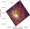 |
Fig. 1 Monoceros R2 as viewed by Herschel: PACS 70 μm in blue; PACS 160 μm in green; and SPIRE 250 μm in red. The image is cropped to the approximate overlap between the PACS and SPIRE maps. The black box indicates the central hub, which is shown in more detail in Fig. 2 (due to the large range in brightness, the detailed features of the central hub do not appear clearly in this three-colour image). The positions of the hub itself, and the three surrounding H ii regions are also given. The three maps are given separately (with intensity scales) in Appendix A. |
2. Observations and data reduction
2.1. Herschel observations
Mon R2 was observed on 4 September 2010, with Herschel, using the SPIRE and PACS instruments. The observations (ObsIDs: 1342204052 and 1342204053) were made as part of the HOBYS Key Project. The maps were made in Parallel Mode, using both PACS and SPIRE simultaneously, with two near-orthogonal (84.8°) scans over the region, scanning at 20′′/s, and covered five wavebands (70 μm, 160 μm, 250 μm, 350 μm, and 500 μm). The bands’ mean beam sizes at this scan speed are 5.6′′, 11.4′′, 18.1′′, 24.9′′, and 36.4′′ (values taken from the PACS Observer’s Manual, v2.5.1 and SPIRE Handbook, v2.5) and their mean noise levels per beam are 7.9 (12.0) mJy, 7.4 (26.8) mJy, 17.6 (7.2) mJy, 10.9 (5.9) mJy, and 12.6 (8.5) mJy respectively (values for Mon R2, with the mean values from the SPIRE PACS Parallel Mode Observers’ Manual in parentheses). The area of overlap between the two instruments’ scans was about 0.85° × 0.85°(or 12 pc × 12 pc), centred on the J2000 coordinates 06h07m30s −06°15′00′′. A Herschel composite map (70 μm, 160 μm, 250 μm) is shown in Fig. 1.
The data were reduced using the Herschel Interactive Processing Environment (HIPE, version 11.1.0; Ott 2010). SPIRE data were reduced using the SPIA (SPIRE Interactive Analysis; Schulz 2011) pipeline. This corrects for relative bolometer gains and then maps the data with the HIPE Destriper, which adjusts the bolometer timelines iteratively until they converge. The SPIRE data used the HIPE point source calibration (Bendo et al. 2013; Griffin et al. 2013). This produces two sets of maps, three calibrated for “point source” emission (in Jy/beam), and three for “extended emission” (in MJy/sr), which have also been given the zero-point emission offset using Planck data. For consistency with PACS, which only calibrates for point sources, in all further analysis only the “point source” maps have been used.
The PACS data were reduced using a HIPE-compatible variant of the Scanamorphos routine (Roussel 2013). Scanamorphos uses the spatial redundancy offered by multiple bolometer scans to estimate the overall emission, but without making any assumptions about the noise model.
The current PACS processing is unable to correct accurately for the diffuse Galactic background levels. The absolute levels can however be approximated by applying offsets taken from Planck data to provide the Herschel maps with background emission offsets, which are assumed for each waveband to remain constant over the mapped region (described in more detail in Bernard et al. 2010). The SPIRE offsets agree very well with those determined using the zero-point correction task in HIPE.
2.2. SCUBA-2 observations
In addition to the Herschel observations, Mon R2 was observed with the SCUBA-2 instrument (Holland et al. 2013) on the JCMT (data provided by D. Nutter). The data provided were used alongside the Herschel data, to provide coverage at longer wavelengths. The region was observed eighteen times between November 2011 and January 2012, as part of the guaranteed time project M11BGT01. Continuum observations at 850 μm and 450 μm were made using fully sampled 1° diameter circular regions (PONG3600 mapping mode; Bintley et al. 2014) at resolutions of 14.1′′ and 9.6′′, respectively. We present the 850 μm observations here.
The data were reduced using the iterative map-making technique makemap in smurf (Chapin et al. 2013), and gridded onto 6′′ pixels at 850 μm. Areas of low emission were masked out based on their signal-to-noise ratio, and a mosaic was formed using this mask to define areas of emission. Detection of emission structure and calibration accuracy are robust within the masked regions, and are uncertain outside of the masked regions.
A spatial filter of 10′ is used in the reduction (described in Pattle et al. 2015). Flux recovery is robust for objects with a Gaussian FWHM less than 2.5′. Objects between 2.5′ and 7.5′ in size will be detected, but both the flux density and the size will be underestimated because Fourier components with scales greater than 5′ are removed by the filtering process. Detection of objects larger than 7.5′ is dependent on the mask used for reduction.
The data are calibrated using the peak Flux Conversion Factor (FCF) of 537 Jy/pW at 850 μm, derived from average values of JCMT calibrators (Dempsey et al. 2013). The PONG scan pattern leads to lower noise levels in the map centre, while data reduction and emission artefacts can lead to small variations in noise level over the whole map.
2.3. IRAM 30-m observations
Mon R2 was also observed with the IRAM 30-m telescope, using the Eight MIxer Receiver (EMIR; Carter et al. 2012), between 12 September and 10 November 2014. The observations were carried out in the on-the-fly observing mode and covered an area of ~100 square arcminutes centred on the J2000 coordinates 06h07m46.2s−06°23′08.3′′, in two frequency bands with coverage of 213.1–220.9 GHz and 228.8–236.6 GHz. The observations thus cover the molecular emission lines of 12CO, 13CO, and C18O 2 → 1, DCN 3 → 2, DCO+3 → 2, and two H2CO lines at 218.22 GHz and 219.16 GHz. In this paper, we only use the C18O 2 → 1 data at 219.56 GHz. The instrument’s pointing and focus were tested every ~2 h against nearby bright quasars. The emission-free reference position is located at 06h08m26.2s−06°33′08.3′′.
The data were reduced with the GILDAS2 software. A baseline of order 1 was subtracted. In order to convert from antenna temperatures (given in this paper) into main beam brightness temperatures, a scaling factor of ~0.6 for the main beam efficiencies3 needs to be applied.
2.4. Other observations
In addition, mid-infrared data were used. These included 24 μm observations with the Multiband Imaging Photometer for Spitzer (MIPS; Rieke et al. 2004; Werner et al. 2004), which were taken from the Spitzer Heritage Archive. Data were also taken from the AllWISE Source Catalog, a catalogue of objects discovered as part of the Wide-field Infrared Survey Explorer (WISE; Wright et al. 2010) and NEOWISE (Mainzer et al. 2011) missions. In both cases, the data were used only to calculate source bolometric luminosities (defined here as the integral of flux densities from 2 μm to 1 mm; Tigé et al. 2017). In addition, 3.6 μm data from Spitzer’s Infrared Array Camera (IRAC; Fazio et al. 2004) were used, solely for source visualisation, as seen in Appendix D. Both Spitzer and WISE are partially saturated at the central hub and cannot be used to determine the luminosities at that location. A full list of wavelengths used for this analysis is given in Table 1.
Telescopes and wavelengths used in the analysis.
3. Overview of the Mon R2 region
Figure 1 shows a three-colour (70 μm, 160 μm, 250 μm) map of the Mon R2 region, and Figs. A.1–A.5 show individual maps at 70 μm, 160 μm, 250 μm, 350 μm, and 500 μm, respectively. In addition, Figs. A.6 and A.7 show the 24 μm MIPS and 850 μm SCUBA-2 data, respectively.
The most striking feature of the Herschel maps of Mon R2 is the central hub, which is very bright in all five wavebands. This region is located at the junction (hence the term “hub”) of several filaments, which are also prominent at most wavelengths. Most of the large-scale filamentary structure emits most strongly at 500 μm, indicating that the filaments consist of cold gas (although the poor spatial resolution at this wavelength makes identification of features significantly easier at shorter wavelengths). However, a significant amount of this filamentary structure (most notably the region to the north-east of the hub) is even visible at 70 μm, especially around the central region, which indicates heating of the filaments, most probably from the associated H ii region.
The central hub itself can be seen in detail in the PACS and shorter wavelength SPIRE bands, as shown in Fig. 2. By inspection, the data appear to contain at least four separate infrared sources, arranged approximately to the north, east, south, and west. Comparison with Beckwith et al. (1976) suggests that these objects approximately correspond to their sources IRS 1 and 4 (south), IRS 5 (north), IRS 3 (east), and another, which was not in the region that they mapped.
The infrared sources appear to be connected, potentially by smaller-scale filamentary structures than those that converge on the central hub, and form a ring-shape around the H ii region in projection, approximately 1′, or 0.24 pc, across. Molecular line observations suggest that this ring is formed by the interactions between the PDR of the H ii region and the denser surrounding material (Pilleri et al. 2013, 2014; Treviño-Morales et al. 2014, 2016). These filaments can be seen to radiate from the central hub in almost all directions. With the help of complementary molecular line data (see Sect. 5) we are able to show that most of the (2D projected) filaments seen in the Herschel data correspond to velocity-coherent objects. The observed velocity gradients suggest that the filaments are gravitationally attracted by the central potential well.
The distance to a reflection nebula can be calculated by finding the distances to the individual stars associated with that nebula. In the case of Mon R2, magnitude measurements of ten individual stars gave a distance of 830±50 pc (Racine 1968). A similar study of thirty stars confirmed this result (Herbst & Racine 1976). A more recent study of over 200 stars in the vicinity found a distance of 905±37 pc, and the even greater (although less precise) value 925±150 pc for the hub alone (Lombardi et al. 2011), and even more recent parallax measurements give a distance of  pc (Dzib et al. 2016). The values show good agreement, with a mean value of about 870 pc. For better comparison with prior literature, the Racine value (830±50 pc) is used throughout this paper. Using a value of 900 pc (in line with the more recent results) would systematically increase our source mass estimates by ~15%.
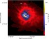 |
Fig. 2 Monoceros R2 central hub region as seen at 160 μm. The region viewed is shown as the black box in Fig. 1. The black circle shows the approximate position and extent of the H ii region (Pilleri et al. 2012; Didelon et al. 2015). The sources are from Beckwith et al. (1976), detected between 1.65 μm and 20 μm (the red object is Mon R2 IRS 1). |
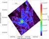 |
Fig. 3 Monoceros R2 high-resolution H2 column density map ( |
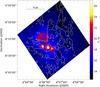 |
Fig. 4 Monoceros R2 dust temperature map. The resolution is as for the 500 μm map (36.4′′). The contours (as for Fig. 3) are at the H2 column densities 7.5 × 1021 cm-2 and 3.5 × 1022 cm-2. |
4. Column density and dust temperature maps
Molecular hydrogen column density and dust temperature maps were obtained by a pixel-by-pixel modified blackbody (greybody) SED fit to the Herschel flux maps. For more details on the SED fit, see Sect. 6. We initially produced three column density maps with different angular resolutions (Σ500, Σ350, and Σ250), which were then used to make a “super-resolution” column density map ( ), using the method given in Palmeirim et al. (2013); a similar method is used in Hill et al. (2012; we note that prior to the procedure, all maps were resampled to the smallest pixel size, 2.85′′). The first column density map, Σ500, was made by smoothing the 160 μm, 250 μm and 350 μm maps to the resolution of the 500 μm map (36.4′′), before fitting the SED to all four maps, giving a column density map with a 36.4′′ resolution. The second column density map, Σ350, was made by smoothing the 160 μm and 250 μm maps to the resolution of the 350 μm map (24.9′′), and then fitting the SED to only these three maps. The third column density map, Σ250, was made by smoothing the 160 μm map to the resolution of the 250 μm map (18.1′′), and using the flux ratio (F250/F160) to create a new temperature map, T250, using the method given in Shetty et al. (2009):
 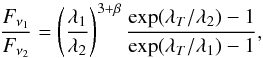 (1)where Fνi are the flux densities at the frequencies νi (or wavelengths λi); β, the dust emissivity index, assumed to be 2; and λT = hc/kT, where: h, c and k are the Planck constant, speed of light and Boltzmann constant, respectively; and T is the dust temperature. T250 was used to find a column density map, Σ250, using the SED equation (Eq. (4) in Sect. 6), and using the 250 μm flux map (and λ = 250 μm). To create the final 18.1′′ resolution column density map, , the three previous column density maps (Σ500, Σ350, and Σ250) were combined, using the following equation:
  (2)where G500_350 and G350_250 are circular Gaussians with FWHMs equal to 26.6′′ (
 ′′) and 17.1′′ (
 ′′). This method ensures that the basic shape of comes from the most reliable of the input column density maps (Σ500, which uses four input flux maps), while the details come from maps with higher resolution but lower reliability (Σ350 and Σ250). To test the reliability of the final map (), it was smoothed to 36.4′′ resolution and compared with the Σ500 map, yielding a difference of <3% over 90% of the region. Unless otherwise stated, the term “column density map” hereinafter refers to this final map (). The final column density and 500 μm dust temperature maps are given in Figs. 3 and 4.
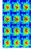 |
Fig. 5 Channel map of C18O 2 → 1 emission. Black contours (2.5–7 K km s-1 by 0.5 K km s-1) are overlaid on the Herschel column density map in colour (Fig. 3). Filaments identified in the C18O and in the Herschel map are classified F1–F8 and traced in grey. |
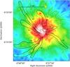 |
Fig. 6 Colour map of the Herschel column density (Fig. 3), overlaid with polygons (F1–F8) indicating the areas over which the filament properties (average column density, density, temperature, and total mass) were determined. The white contours show the filaments identified by getsources in the column density map. |
Looking at the column density map, the highly filamentary nature of the region can be clearly seen. The filaments correspond well to column densities above 7.5 × 1021 cm-2 (white contour), while the central hub corresponds well to column densities above 3.5 × 1022 cm-2 (black contour). Meanwhile, in the dust temperature map, it can be seen that the filamentary regions often correspond to lower temperatures (as expected, since a dense region will be better shielded from external radiation), while warmer regions (especially the northern and eastern H ii regions) can be seen to correspond to lower-density regions (both because the heating influence can spread farther in lower densities and also because the H ii regions will naturally reduce their own local densities). This trend is inverted at the centre of the hub, which has the highest dust temperature in the region (this corresponds to the central UCH ii region). This is potentially because the UCH ii region has not yet had time to disperse its high-density surroundings; more examples of this are seen in NGC 6334 (Russeil et al. 2013; Tigé et al. 2017), W48A (Rygl et al. 2014) and part of the DR21 ridge (Hennemann et al. 2012). It should be noted that while the column density is two-dimensional (2D), and thus not completely analogous to the true three-dimensional (3D) molecular density, for a region with no significant foreground or background emission (such as Mon R2), it can be assumed that high–column-density regions are regions of actual high density.
5. Velocity structure
As described in Sect. 2.3, extended maps of isotopomeric CO 2 → 1 and 1 → 0 lines have recently been obtained with the IRAM 30-m telescope (PIs N. Schneider, A. Fuente, S. Treviño-Morales). We present here C18O 2 → 1 data from these projects, which are fully shown and discussed in Treviño-Morales (2016), and in Rayner (2015). It should be noted that we do not aim to perform explicit filament detections and analyses here. Rather, we intend to show that what appear as filaments in projected column density do indeed correspond to coherent velocity features, and can be used to derive first order approximations of their physical properties.
Figure 5 shows a channel map of C18O emission overlaid on the column density map obtained with Herschel. The black contours of C18O emission trace very well, in some velocity intervals, the filaments seen with Herschel and reveal velocity gradients that are potentially caused by inflow along inclined filaments. All clear correspondences are labelled (filaments F1–F8; identified by eye from the C18O structures). Fainter filamentary structures that are only seen in the Herschel map were not considered for our census, even though they are partly identified in lower-density tracers such as 12CO 1 → 0.
We note that these filaments do not exactly correspond to the filaments detected by the getsources routine (see Appendix B), which are detected by measuring large-scale but low width objects on the column density maps. The main reason for this discrepancy is not the method of identification, but rather the fact that the C18O filaments have been identified across multiple molecular line maps, while the getsources filaments have been identified only on the column density map. Consequently, a one-to-one correlation would not be expected, both because C18O does not directly trace dust column density, and also because the by-eye detection focuses on filaments that are coherent structures in velocity space, rather than 2-dimensional column density.
The two different sets of filaments are compared in Fig. 6, with the C18O filaments in black, and the getsources filaments in white. There is reasonably good overlap in most cases, especially filament F2 (to the north-east) and F6 (to the south). Only two of the C18O filaments are not detected by getsources, F3 (to the north) and F7 (to the south-east), and the former is certainly visible by eye.
One of the best examples of a velocity gradient is in F2, which shows its first emission close to to the cluster centre at 11.5 km s-1. The C18O emission then shifts towards north-east “along” the Herschel filament until a velocity of 9.5 km s-1. This emission pattern is consistent with infall along a filament that is inclined towards the observer (although outflow along a filament inclined away from the observer is also a possibility). For other filaments, for example, F8, the top of the column lies at higher positive velocities, indicating that this part of the filament is tilted away from the observer (again, assuming infall). Overall, the northern filaments (F1–F4) appear visually more collimated than the southern ones (F6–F8). As outlined below, the two filament groups also differ in their physical properties. The more widespread C18O emission close to the central region in the velocity range 10.2–8.9 km s-1 can be interpreted as filaments seen head-on.
For all filaments, we determined the velocity gradient relative to the observer, Δvgrad, from the channel map in order to derive dynamical lifetimes and infall rates. We assume a random distribution of orientation angles and thus an average angle to the line-of-sight of 57.3° (Schneider et al. 2010) meaning that the dynamical lifetime tl of the filament is calculated as tl = l/ (Δvgradtan(57.3)). The infall rate Ṁ is then Ṁ = M/tl with the mass M obtained from the Herschel maps. For the mass estimate, we defined polygons around the filament skeletons identified in the C18O map and approximately following the filaments seen on the column density map, with similar widths (~25′′, or ~0.1 pc). These are shown in Fig. 6. The background around the filaments is highly variable, ranging from ~1021 cm-2 over most of the region to over 4 × 1022 cm-2 at the central hub, approximately 50% of the column density values measured over the filaments. Since the majority of the mass in the filaments comes from the central hub, this suggests that a reasonable lower limit for the masses is 50% of the total measured value (which was used as the upper limit). As this is an estimate, no further background subtraction was performed. From this point, the upper limit value is used.
We also estimated the average column density N, the average density n, the mass per unit length Ml, and the average dust temperature T from the Herschel data. The critical mass per unit length Ml,crit above which filaments become gravitationally unstable (Arzoumanian et al. 2011) was determined following Ostriker (1964): ![Mathematical equation: \begin{equation} M_{l,\mathrm{crit}}~=~\frac{2\,c^2_{\rm s}}{G}~=~1.67~T~~[M\msun\,{\rm pc}^{-1}]. \label{Eqn:critmass} \end{equation}](/articles/aa/full_html/2017/11/aa30039-16/aa30039-16-eq67.png) (3)For the sound speed cs we assume isothermal gas (of temperature T) where the ideal gas equation of state holds and thus
(3)For the sound speed cs we assume isothermal gas (of temperature T) where the ideal gas equation of state holds and thus  with the Boltzmann constant k and the mean molecular weight per free gas particle μ = 2.33 (accounting for 10% He and trace metals).
The physical properties of the filaments are reported in Table 2. The masses of the filaments range between 26 and 114 M⊙ per parsec, and are thus a factor of ~10 less massive (though only a factor of 2 shorter) than the filaments linked to the DR 21 ridge (100–3700 M⊙ pc-1; Schneider et al. 2010; Hennemann et al. 2012) and a factor of ~3 less massive than the Serpens South filament (62–290 M⊙ pc-1; Hill et al. 2012; Kirk et al. 2013a), but of a similar mass per unit length to many other regions’ filaments (~20–100 M⊙ pc-1, in regions as diverse as Aquila, Polaris, and IC 5146; André et al. 2014).
The filaments fall onto central hub, which, with a mass of ~1000 M⊙, is many times more massive than even the most massive of the filaments. The average temperature within the filaments ranges between 15 and 19.5 K. The southern filaments F6, F7, and F8 are colder (around 15 K) than the northern ones (around 19 K). All upper limit masses for the filaments are supercritical (Ml>Ml,crit) and thus gravitationally unstable and only three of the eight filaments have subcritical lower-limit masses.
Assuming that the full velocity gradient corresponds to infall, the dynamic lifetimes of the filaments are short, between 1.6 and 5.6 × 10⁵ yr, and the mass infall rates range between 0.5 and 3.25 × 10⁻⁴ M⊙/yr. The southern filaments have lower infall rates than the northern ones. If a constant average infall rate of 1.4 × 10⁻³ M⊙/yr over time is assumed, it takes ~0.7 × 10⁶ yr to build up a central hub of 1000 M⊙, the current mass of the central region. Using the lower-limit mass values, this value would be approximately doubled, to ~1.4 × 10⁶ yr. This is of course a rough estimate and the timescale is probably lower because we consider only a few prominent filaments, mostly oriented in the plane of the sky, and ignore all head-on ones and fainter filaments. Nevertheless, a value of about 106 yr indicates that the formation of ridges and hubs starts already at a very early phase during molecular cloud formation. This is consistent with a scenario in which these massive regions are formed out of initially atomic flows that quickly transform into filaments, which then supply the mass by means of gravitational contraction onto the hub (Heitsch 2013a,b).
Properties of the filaments F1–F8.
6. Source detection and classification
The source detection and classification process was carried out according to the standard procedures of the HOBYS group, as outlined in Tigé et al. (2017). To identify the positions of compact objects, we used the getsources routine (version 1.140127; Men’shchikov et al. 2012; Men’shchikov 2013) which uses maps at all Herschel wavelengths simultaneously. An account of the workings of this routine is given in Appendix B. The observed maps input to the routine were the five Herschel maps (70 μm, 160 μm, 250 μm, 350 μm, and 500 μm) and two ancillary maps (MIPS 24 μm and SCUBA-2 850 μm). Three derived maps are also used as input to getsources: the high-resolution column density map (), and two others, versions of the 160 μm and 250 μm maps corrected for the effects of temperature. These are created by using the colour-temperature map, T250, to remove the effects of temperature from the 160 μm and 250 μm maps (these maps are used for detection in place of the observed 160 μm and 250 μm maps, but measurements are only taken from the original maps). We note that neither the 24 μm nor the 850 μm maps were used for detection, since the former contains many sources that are not seen at longer wavelengths, which could add unwanted MIR sources to the output catalogue, and the latter is noisy due to atmospheric effects, which could cause errors in position measurement.
To test the completeness of getsources in Mon R2, we injected additional synthetic sources into the maps, and the routine was run again on these source-injected maps. The getsources extraction was performed identically to the extraction described above, even including the column density and temperature-corrected maps. This test suggested that ~70% of sources over 1 M⊙ would have been detected. Five further extractions were performed on the central hub alone; in each extraction only a small number of sources was added so as not to increase the crowding in the region too much. This test suggested that, within the central hub, only ~33% of sources over 1 M⊙ would have been detected. More details of the completeness test are given in Appendix C.
In the Mon R2 region, getsources detected 555 sources, but even though these were all detected to a (detection) signal-to-noise level of 5σ, only the most robust sources (as described below, and in Tigé et al. 2017) are counted in the final catalogue. First, sources were removed from the getsources catalogue if they were at the edge of the map. In addition, each wavelength detection for each source was designated “reliable” if its peak intensity (measurement) signal-to-noise ratio and its total flux density (measurement) signal-to-noise ratio were both over two, and its axis ratio was under two. Sources were removed from the catalogue if they did not have reliable measurements at either 160 μm or 250 μm. In order to find a single value for the “size” of the sources, the geometric mean of the measured major and minor FWHM sizes was found for each wavelength. These values were then deconvolved with the wavelengths’ beam sizes, with a minimum value set to half the beam size. The reference size (Θ) was defined as the smaller of the deconvolved sizes at 160 μm and 250 μm, in the case where both wavelengths had reliable detections, or the size at the reliable wavelength (out of 160 μm and 250 μm), in the case where only one of the two was reliable.
Sources were treated as “robust” if they had reliable detections at three wavelengths over 100 μm (one of which, as mentioned above, had to be at either 160 μm or 250 μm). Finally, sources were removed due to poor SED fits, and due to being likely extraction artefacts (both described in more detail below), leaving 177 “robust” sources. For the remainder of the paper, only these robust sources are considered.
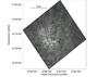 |
Fig. 7 Monoceros R2 sources, on the 250 μm flux map (Fig. A.3). The getfilaments map is overlaid as black contours (strictly, these are the filaments detected on the column density map at scales below 72′′). The contours are those from Fig. 3 (H2 column densities 3 × 1021 cm-2 and 1.5 × 1022 cm-2). A zoom-in of the region in the red box (the central hub) is shown in Fig. 8. The points are protostars (blue), bound cores (green), and unbound clumps (red); see text for details. |
From the measured flux densities, the spectral energy distribution (SED) of each robust source can be constructed. The SED is assumed to fit a greybody with the following form (Chapin et al. 2008): 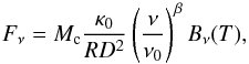 (4)where Fν is the observed flux density (here and elsewhere in this paper) at frequency ν; Mc is the source gas mass; κ0 is the dust absorption coefficient, measured at a reference frequency ν0; R is the assumed mass ratio of gas to dust in the cloud; β is the dust emissivity index; and Bν(T) is the Planck function, with temperature T. Although β, R and κ0 are subject to significant uncertainties, there exist common approximations based on measurements made in the literature. It has been suggested that the emissivity index, β, varies between 1 for higher frequencies (wavelengths below 250 μm) and 2 for lower frequencies (above 250 μm; Hildebrand 1983); a value of β = 2 is generally used in Herschel SAG34 papers (including Motte et al. 2010; Hennemann et al. 2010; Könyves et al. 2010; Giannini et al. 2012). The gas-to-dust ratio is generally taken to be R = 100 (Beckwith et al. 1990), or in other words, the dust is assumed to make up about 1% of the cloud by mass. The absorption coefficient, κ0, is set to 10 cm2 g-1 (or 0.1 cm2 g-1 when divided by the gas-to-dust ratio) at a reference frequency of 1 THz (or a wavelength of 300 μm); this has been found to have an accuracy of better than 50% over column densities between 3 × 1021 cm-2 and 1023 cm-2 (Roy et al. 2014). The distance to Mon R2, 830 pc, is discussed in Sect. 3.1. Based on these assumptions, the source’s mass and temperature can be found from the best SED fit (in this case, using the MPFIT routine; Markwardt 2009).
Before the SED can be fit, there is another correction that needs to be made. The total fluxes for wavelengths of 160 μm or greater are scaled for the source size (since the fluxes were measured over variable apertures), so that: 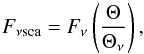 (5)where Θν is the deconvolved FWHM at frequency ν. This flux scaling process is introduced in Motte et al. (2010) and explained in more detail in Nguyen Luong et al. (2011). It should be noted that the flux scaling is merely an estimate, and does not account for more complex internal core structure (such as subfragmentation or density flattening). It is also a practical/empirical approach, and while it does generally give better-fitting SEDs, it is likely to increase the uncertainty of the values. In order to provide a test for flux scaling, SEDs were also constructed using flux measured by aperture photometry on maps convolved to the 500 μm resolution (36.4′′). The rms of the relative difference between the mass calculated by this method and the mass calculated using flux scaling was found to be 1.17 (strictly, the rms of (M − Mconv) /M, where M is the mass calculated by flux scaling, and Mconv is the mass calculated using the convolved fluxes; the fluxes used and masses measured are provided in the catalogue files). This suggests that an error of ~20% should be applied to the masses, in addition to the mass errors calculated purely from the fitting routine (the error due to the fit alone is given in the catalogue as Merr_fit), and the 15% systematic uncertainty from the distance measurements. We note that colour corrections were not performed, as any correction applied would be smaller than the uncertainties likely introduced by flux scaling.
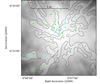 |
Fig. 8 Zoom in on the central hub region of Fig. 7. The contour shows the filaments as detected by getsources on the column density map. |
For the SED fitting, all reliable detections (as defined earlier) above 100 μm are included in the fit. The errors on each wavelength are the total flux error, as measured by getsources, summed in quadrature to the instrumental and calibration errors (10% of the flux for all bands). Wavelengths that are not reliable due to the source shape are included as “1σ upper-limits”, meaning that the error is set equal to the flux itself; meanwhile, wavelengths that are not reliable due to having flux below 2σ have the flux itself (along with the errors) set to the 2σ value. The 70 μm data are fit only to those sources that show a temperature of over 32 K when fit without it. This is necessary, since such SEDs are poorly described by wavelengths of 160 μm and above alone. As mentioned above, fits (both including and excluding 70 μm) with reduced χ2 values above 10 are also excluded from the final catalogue, since the fits (and thus output parameters) provided are dubious (only about 10% of the total number removed were cut due to this requirement alone). It should be noted that the 24 μm flux is only used to calculate the luminosity, and takes no part in the SED determination.
In addition to the getsources fluxes, WISE all-sky catalogue data are used to provide mid-infrared coverage for luminosity calculation. All WISE sources within 6′′ of the centre of the detected Herschel source are assumed to contribute. The mid-infrared luminosity is derived by calculating the integral of the WISE fluxes, the 24 μm flux and the 70 μm flux. The far-infrared luminosity is the integral of the SED between 70 μm and 1200 μm.
Sources are classified as protostars if they have both a reliable detection at 70 μm and either a reliable detection at 24 μm, or are present in the WISE catalogue (the second requirement was lifted for sources in the central region, as the 24 μm MIPS data and two of the four WISE bands are saturated here). In addition, the source FWHM at 70 μm is required to be under 11.6′′ (twice the 70 μm beam size). A non-protostellar (or starless) source is classified as gravitationally bound if its reference size (Θ) is less than twice its Bonnor radius (the radius of a critically dense Bonnor-Ebert sphere with the same mass and temperature), which is given by: 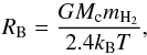 (6)where G and kB are the gravitational and Boltzmann constants and mH2 is the average molecular mass (Bonnor 1956). All other robust sources were classified as either gravitationally unbound or “undefined cloud structures” (Tigé et al. 2017), a designation for objects detected by getsources, but not associated with either a protostar or a peak in column density. These are potentially artefacts of the extraction, especially given that they are generally associated with the most crowded parts of the region. Consequently, these objects are not included in the catalogue or the analysis.
The positions of these sources are shown in Fig. 7, overlaid on a filament map taken from getsources (strictly, this is the map of filaments detected at scales under 72′′, or 0.3 pc, on the column density map). As can be seen, the majority (60%, or 109 out of 177) of sources are coincident with the getsources filaments. In addition, the sources are mainly clustered around the central hub (as shown in Fig. 8), with 29 robust sources detected there (80%, or 23 of them, on getsources filaments).
The basic parameters of the overall source dataset (temperature, mass, bolometric luminosity, and reference size) are given in Table 3. We note that not all of the bound cores are likely to be true prestellar cores; although such objects could be detected separately at this distance (the 160 μm resolution is ~0.05 pc at Mon R2, while prestellar cores have sizes of 0.1–0.2 pc; Roy et al. 2014), the larger bound cores are potentially clusters of several prestellar cores. These are likely to be on the path to star formation.
Numbers (N) and parameter ranges for all robust sources.
As can be seen from Table 3, those sources in the central hub (defined here by the N-PDF excess from Schneider et al. 2015, which is equivalent to column densities above 3.5 × 1022 cm-2) are both hotter and more luminous than those outside. There appears to be a difference in the mass ranges, too, with the more massive sources found in the hub. This effect is partly due to the high completeness limit of getsources in the hub region (see Appendix C), which could only reliably detect a third of sources above 1 M⊙ due to the high crowding and confusion.
One single source (HOBYS J060740.3 −062447) has a mass above 20 M⊙, and is thus potentially a true high-mass star in formation. At the edge of the hub region, it is associated with the young star 2MASS J06074062−0624410, and appears to overlap with the western H ii region (although this may be a projection effect). A further eleven sources have masses over 10 M⊙, meaning that they are potentially intermediate-mass stars (final mass ≳5 M⊙) in formation. Four of these sources are larger objects in the outer parts of the region. While they are all massive enough to be gravitationally bound, none are particularly dense, with densities of 2.2 × 10³–6.0 × 104 cm-3 (for comparison, the density of HOBYS J060740.3 −062447 is 9.0 × 105 cm-3). The remaining seven sources are (like HOBYS J060740.3 −062447) within (or close to) the ≳3.5 × 1022 cm-2 column density hub, and include HOBYS J060746.1 −062312, which is associated with Mon R2 IRS 1. These objects are mainly bound dense cores, with densities of 6.2 × 10⁴–2.1 × 106 cm-3. The properties of these sources are given in the lowest rows of Table 3, and the individual properties are given in the tables in Appendix D (measured properties) and Table 4 (derived properties).
Derived core properties.
Looking at total masses, we can see that the sources in the central hub (total mass ~220 M⊙) make up about half of the mass of sources in the region (total mass ~580 M⊙), even though they account for less than a quarter by number. Taking completeness into account, we find an even greater discrepancy, with potentially 620 M⊙ in central hub sources, two thirds the completeness-corrected mass of all sources in the region (980 M⊙). From the column density map, we can see that the total masses of material in the regions are approximately 2200 M⊙ (central) and 30 000 M⊙ (total), meaning that 10–30% of the central region is associated with star-forming cores, compared to only 2–4% of the total region. Such behaviour has been seen in other high density regions, including the W43 ridge (Louvet et al. 2014).
7. Source properties in and outside the central hub
Contrasting the parameters of the sources inside the central hub with those outside it, a difference can be seen. Plots of bolometric luminosity and reference size against mass are shown in Figs. 9 and 10, respectively, and they show that the central hub sources (filled shapes) are generally smaller, more luminous, and potentially even more massive than those outside the hub, occupying distinct locations on each plot (masses over ~2 M⊙; luminosities over ~10 L⊙; reference size under ~0.04 pc). The luminosity-mass plot shows evolutionary tracks for four protostars of final protostellar mass (M) 0.6 M⊙, 2 M⊙, 8 M⊙, and 20 M⊙ (from Duarte-Cabral et al. 2013; Duarte-Cabral, priv. comm.), in which Lbol = L∗ + GϵMM∗/τR∗, where: L∗, M∗, and R∗ are the luminosity, mass, and radius of the protostar itself; G is the gravitational constant; ϵ is the efficiency for an individual core’s formation (the fraction of the core that eventually joins the protostar), set to 50%; and τ is the characteristic timescale for protostellar evolution, set to 105 yr (André et al. 2008; Tigé et al. 2017).
The objects from the central hub seem to be segregated from those in other parts of the region, with the inner objects generally located above the 2 M⊙ evolutionary track, and the majority of outer objects located below the track. In addition, those outer objects above 2 M⊙ appear to show a segregation based on evolutionary level, with the inner objects being exclusively located at the start of the tracks. This suggests that these objects form a secondary population within the region, one that potentially began evolution significantly earlier than those outside the hub. This is in contrast to what was seen in Cygnus X (Duarte-Cabral et al. 2013), in which the massive objects are far less evolved than the lower-mass objects, suggesting that for the Cygnus X region, at least, the massive star formation occurring is comparatively more recent than in Mon R2. The different types of objects found outside the central hub (protostellar, bound, or unbound) all occupy distinct positions in the two plots (albeit with some overlap); those inside show no such differentiation. Similarly, the size-mass positions show a distinction between the hub sources (small and massive) and the outer sources, which can have similar masses, but only with much lower densities.
It should be noted that the tracks represent the evolution of objects heated only from within; the externally heated bound cores in the central hub are likely to be higher up the tracks than they would be in isolation. While this could affect the positions of such sources in Fig. 9, it does not explain their small size and high mass, as seen in Fig. 10. This positioning can be partially explained by the high completeness limit of the central hub (see Appendix C), as less massive, less luminous, and larger sources within the central hub will be missed simply due to the complexity of the region. The number of sources missed in the central hub (66% above 1 M⊙ and 80% above 0.1 M⊙; likely over a hundred in total) could certainly explain the absence of central hub sources in the high-size, low-mass and low-luminosity parts of the plots. The poor completeness of the central hub does not, however, explain the absence of “outer” sources (sources from outside the hub in the low-size, high-mass and high-luminosity parts of the plots; indeed, the completeness tests suggest that 90% of sources under 0.035 pc and over 1 M⊙ have been detected in the outer regions. Only four such sources have been found outside the central hub (~3%), while eighteen of the central hub sources (~62%) fit these parameters. If the ratios were equivalent, then over 500 extra sources over 0.1 M⊙ would be needed in the central hub, rather than the 150 suggested by the completeness analysis. This at the very least suggests that the central hub of Mon R2 has an abundance of these objects when compared to the surroundings, and that the source populations are indeed different. Such crowding of high-mass protostars has also been observed in HOBYS ridges (Hill et al. 2011; Nguyen Luong et al. 2011; Louvet et al. 2014).
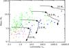 |
Fig. 9 Bolometric luminosity-mass plot for robust sources in Mon R2. The coloured symbols represent protostars (blue diamonds), bound cores (green squares), and unbound clumps (red triangles). Filled shapes are sources within the central hub. The black lines represent evolutionary tracks for protostars with final protostellar masses of 0.6 M⊙, 2 M⊙, 8 M⊙, and 20 M⊙ (described in Sect. 7). |
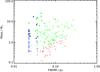 |
Fig. 10 Mon R2 plot of mass against reference size (full width at half maximum at either 160 μm or 250 μm; defined in Sect. 6). As for Fig. 9. The two lines of protostellar (blue) sources are at half the 160 μm and 250 μm beam sizes (5.7′′ and 9.1′′, respectively, corresponding to sizes 0.023 pc and 0.037 pc), which were taken as the minimum source sizes (see Sect. 6 for more details). |
These features suggest a region in which star formation initially begins at the meeting-point of a network of filaments (the hub), and commences in the outer regions at a later time. It is also possible that the star-formation occurring in the central hub is fuelled by material from the filaments themselves, which would in turn partially deplete star-forming material in the surrounding areas making it harder for stars to form in surrounding regions. It is possible that the surrounding H ii regions played a part in the formation of the central hub by providing external pressure to enhance the gravitational collapse, although it is unlikely to have played a major part (Didelon et al. 2015). The ionising stars of these three regions are young B types (BD−06 1415, B1; BD−06 1418, B2.5V; HD 42004, B1.5V; Racine 1968; Reed 2003) that are too evolved to be detected by Herschel and getsources. Their probable masses (~10 M⊙ for a B1–2 type star; Habets & Heintze 1981) would thus mean that at least some intermediate-to-high mass star formation must have occurred in the region prior to the formation of the hub, but the environment at the time of their forming is impossible to determine. The three stars are all at most ~2 pc from the edge of the hub region (assuming minimal projection effects), which, given the age of the region (~5 × 10⁶ yr as determined here, which is of the same order of magnitude as that of Didelon et al. 2015, ~106 yr), could allow the stars to have begun forming in the vicinity of the hub, before moving to their current positions at velocities of no more than 1 km s-1. Indeed, there is already a sizable population of young stars (~1 Myr) already in existence at the Mon R2 central hub, with at least 300 stars (and likely over 500) detected over the entire hub (Carpenter et al. 1997) and almost 200 detected in the central square arcminute (approximately coincident with the H ii region shown in Fig. 2; Andersen et al. 2006).
Mon R2 is an unusual, but not necessarily unique, region; as mentioned earlier, both Cep OB3 and NGC 6334 show similar N-PDF excesses (Schneider et al. 2015), as do W3 (Rivera-Ingraham et al. 2015), and NGC 2264 (Rayner 2015), the latter of which also showing a similar split in its source population, although without any obvious filamentary hub. While both W3 and NGC 6334 are more than twice as distant as Mon R2, and thus their internal structure (both sources and filaments) is significantly harder to resolve, both Cep OB3 and NGC 2264 are at similar distances to Mon R2, and thus follow-up studies on these two regions could help add to the observations from Mon R2. Other high-density ridges, such as those in W43 (Louvet et al. 2014) and Cygnus X (Hennemann et al. 2012) could also provide similar excesses, even though neither has been examined for the N-PDF excess. Cygnus X could thus provide another region for follow-up studies, although as W43 is more than six times as distant as Mon R2, it is unlikely to have sufficient resolution to rival Cep OB3 or NGC 2264.
8. Conclusions
In Mon R2, we detect 177 robust sources, including 28 protostars and 118 bound cores. About a sixth of these by number (29: 11 protostars and 18 bound cores) and a third by mass (200 M⊙, out of 540 M⊙) are found in a filamentary hub structure at the centre of the region. These sources are also smaller and more luminous (on average), and thus likely more highly evolved, than the sources in the outer regions, and while this is partly attributable to poor completeness in the central hub, this cannot account entirely for the difference.
In addition, the central hub was observed in C18O, giving the kinematics of the system. Matter is observed to be moving along the filaments, with mass infall rates of ~2 × 10⁻⁴ M⊙/yr, indicating that the ~1000 M⊙ central hub has likely been forming for ~5 × 10⁶ yr, a significant portion of the lifetime of the molecular cloud.
This all comes together to suggest a model in which the hub forms very early in the life of the molecular cloud (although it itself may have been formed by young stars forming around it), being fed by infall from filaments around it. It then began star formation in advance of the rest of the region, fuelled by the increased densities there. In addition, it is possible that material flowing into the hub from the filaments could decrease the amount of star formation in surrounding regions.
Herschel is an ESA space observatory with science instruments provided by European-led Principal Investigator consortia and with important participation from NASA.
A SPIRE Consortium Specialist Astronomy Group which implemented the HOBYS and Herschel Gould Belt surveys.
Acknowledgments
We are grateful for the comments of an anonymous referee, which have helped us to improve this paper. The Herschel spacecraft was designed, built, tested, and launched under a contract to ESA managed by the Herschel/Planck Project team by an industrial consortium under the overall responsibility of the prime contractor Thales Alenia Space (Cannes), and including Astrium (Friedrichshafen) responsible for the payload module and for system testing at spacecraft level, Thales Alenia Space (Turin) responsible for the service module, and Astrium (Toulouse) responsible for the telescope, with in excess of a hundred subcontractors. SPIRE has been developed by a consortium of institutes led by Cardiff Univ. (UK) and including Univ. Lethbridge (Canada); NAOC (PR China); CEA, LAM (France); IFSI, Univ. Padua (Italy); IAC (Spain); Stockholm Observatory (Sweden); Imperial College London, RAL, UCL-MSSL, UKATC, Univ. Sussex (UK); Caltech, JPL, NHSC, Univ. Colorado (USA). This development has been supported by national funding agencies: CSA (Canada); NAOC (PR China); CEA, CNES, CNRS (France); ASI (Italy); MCINN (Spain); SNSB (Sweden); STFC and UKSA (UK); and NASA (USA). PACS has been developed by a consortium of institutes led by MPE (Germany) and including UVIE (Austria); KUL, CSL, IMEC (Belgium); CEA, OAMP (France); MPIA (Germany); IFSI, OAP/AOT, OAA/CAISMI, LENS, SISSA (Italy); IAC (Spain). This development has been supported by the funding agencies BMVIT (Austria), ESA-PRODEX (Belgium), CEA/CNES (France), DLR (Germany), ASI (Italy), and CICT/MCT (Spain). HIPE is a joint development by the Herschel Science Ground Segment Consortium, consisting of ESA, the NASA Herschel Science Center, and the HIFI, PACS and SPIRE consortia. This work is based in part on observations made with the Spitzer Space Telescope, obtained from the NASA/IPAC Infrared Science Archive, both of which are operated by the Jet Propulsion Laboratory, California Institute of Technology under a contract with NASA. IRSA and the Spitzer Heritage Archive utilize technology developed for the Virtual Astronomical Observatory (VAO), funded by the National Science Foundation and NASA under Cooperative Agreement AST-0834235. The James Clerk Maxwell Telescope has historically been operated by the Joint Astronomy Centre on behalf of the Science and Technology Facilities Council of the United Kingdom, the National Research Council of Canada, and the Netherlands Organisation for Scientific Research. Additional funds for the construction of SCUBA-2 were provided by the Canada Foundation for Innovation. This research has made use of the SIMBAD database, operated at CDS, Strasbourg, France. This publication makes use of data products from the Wide-field Infrared Survey Explorer, which is a joint project of the University of California, Los Angeles, and the Jet Propulsion Laboratory/California Institute of Technology, and NEOWISE, which is a project of the Jet Propulsion Laboratory/California Institute of Technology. WISE and NEOWISE are funded by the National Aeronautics and Space Administration. N.S. acknowledges support by the ANR-11-BS56-010 project “STARFICH”. Part of this work was supported by the French National Agency for Research (ANR) project “PROBeS”, number ANR-08-BLAN-0241. N.S. acknowledges support by the DFG through project number Os 177/2-1 and 177/2-2 and central funds of the program 1573 (ISM-SPP). G.J.W. gratefully acknowledges support from the Leverhulme Trust. S.P.T.M. and A.F. thank the Spanish MINECO for funding support from grants AYA2012-32032, CSD2009-00038, FIS2012-32096, and ERC under ERC-2013-SyG, G. A. 610256 NANOCOSMOS. This work has received support from the ERC under the European Union’s Seventh Framework Programme (ERC Advanced Grant Agreements No. 291294 – “ORISTARS”).
References
- Andersen, M., Meyer, M. R., Oppenheimer, B., Dougados, C., & Carpenter, J. 2006, AJ, 132, 2296 [NASA ADS] [CrossRef] [Google Scholar]
- André, P., Minier, V., Gallais, P., et al. 2008, A&A, 490, L27 [NASA ADS] [CrossRef] [EDP Sciences] [Google Scholar]
- André, P., Men’shchikov, A., Bontemps, S., et al. 2010, A&A, 518, L102 [NASA ADS] [CrossRef] [EDP Sciences] [Google Scholar]
- André, P., Di Francesco, J., Ward-Thompson, D., et al. 2014, Protostars and Planets VI, 27 [Google Scholar]
- Arzoumanian, D., André, P., Didelon, P., et al. 2011, A&A, 529, L6 [Google Scholar]
- Bally, J., & Lada, C. J. 1983, ApJ, 265, 824 [NASA ADS] [CrossRef] [Google Scholar]
- Beckwith, S., Evans II, N. J., Becklin, E. E., & Neugebauer, G. 1976, ApJ, 208, 390 [NASA ADS] [CrossRef] [Google Scholar]
- Beckwith, S. V. W., Sargent, A. I., Chini, R. S., & Güsten, R. 1990, AJ, 99, 924 [NASA ADS] [CrossRef] [Google Scholar]
- Bendo, G. J., Griffin, M. J., Bock, J. J., et al. 2013, MNRAS, 433, 3062 [NASA ADS] [CrossRef] [Google Scholar]
- Benedettini, M., Schisano, E., Pezzuto, S., et al. 2015, MNRAS, 453, 2036 [NASA ADS] [CrossRef] [Google Scholar]
- Bernard, J.-P., Paradis, D., Marshall, D. J., et al. 2010, A&A, 518, L88 [NASA ADS] [CrossRef] [EDP Sciences] [Google Scholar]
- Bertin, A., Mellier, Y., Radovich, M., et al. 2002, in Astronomical Data Analysis Software and Systems XI, ASP Conf. Ser., 281, 228 [NASA ADS] [Google Scholar]
- Bintley, D., Holland, W. S., MacIntosh, M. J., et al. 2014, SPIE Conf. Ser., 9153, 3 [Google Scholar]
- Bonnell, I. A., & Bate, M. R. 2006, MNRAS, 370, 488 [NASA ADS] [CrossRef] [Google Scholar]
- Bonnor, W. B. 1956, MNRAS, 116, 351 [CrossRef] [Google Scholar]
- Carpenter, J. M., Meyer, M. R., Dougados, C., Strom, S. E., & Hillenbrand, L. A. 1997, AJ, 114, 198 [NASA ADS] [CrossRef] [Google Scholar]
- ; Erratum: 1997, AJ, 114, 1275 [NASA ADS] [CrossRef] [Google Scholar]
- Carter, M., Lazareff, B., Maier, D., et al. 2012, A&A, 538, A89 [NASA ADS] [CrossRef] [EDP Sciences] [Google Scholar]
- Chapin, E. L., Ade, P. A. R., Bock, J. J., et al. 2008, ApJ, 681, 428 [NASA ADS] [CrossRef] [Google Scholar]
- Chapin, E. L., Berry, D. S., Gibb, A. G., et al. 2013, MNRAS, 430, 2545 [NASA ADS] [CrossRef] [Google Scholar]
- Condon, J. J., Cotton, W. D., Greisen, E. W., et al. 1998, AJ, 115, 1693 [NASA ADS] [CrossRef] [Google Scholar]
- Cutri, R. M., Skrutskie, M. F., van Dyk, S., et al. 2003, VizieR Online Data Catalog: II/246 [Google Scholar]
- De Graauw, T., Helmich, F. P., Phillips, T. G., et al. 2010, A&A, 518, L6 [NASA ADS] [CrossRef] [EDP Sciences] [Google Scholar]
- Dempsey, J. T., Friberg, P., Jenness, T., et al. 2013, MNRAS, 430, 2534 [Google Scholar]
- Di Francesco, J., Johnstone, D., Kirk, H., MacKenzie, T., & Ledwosinska, E. 2008, ApJS, 175, 277 [NASA ADS] [CrossRef] [Google Scholar]
- Didelon, P., Motte, F., Tremblin, P., et al. 2015, A&A, 584, A4 [NASA ADS] [CrossRef] [EDP Sciences] [Google Scholar]
- Dierickx, M., Jiménez-Serra, I., Rivilla, V. M., & Zhang, Q. 2015, ApJ, 803, 89 [NASA ADS] [CrossRef] [Google Scholar]
- Duarte-Cabral, A., Bontemps, S., Motte, F., et al. 2013, A&A, 558, A125 [NASA ADS] [CrossRef] [EDP Sciences] [Google Scholar]
- Dzib, S. A., Ortiz-León, G. N., Loinard, L., et al. 2016, ApJ, 826, 201 [NASA ADS] [CrossRef] [Google Scholar]
- Fallscheer, C., Reid, M. A., Di Francesco, J., et al. 2013, ApJ, 773, 102 [NASA ADS] [CrossRef] [Google Scholar]
- Fazio, G. G., Hora, J. L., Allen, L. E., et al. 2004, ApJS, 154, 10 [NASA ADS] [CrossRef] [Google Scholar]
- Fuente, A., Berné, O., Cernicharo, J., et al. 2010, A&A, 521, L23 [NASA ADS] [CrossRef] [EDP Sciences] [Google Scholar]
- Giannini, T., Elia, D., Lorenzetti, D., et al. 2012, A&A, 539, A156 [NASA ADS] [CrossRef] [EDP Sciences] [Google Scholar]
- Griffin, M. J., Abergel, A., Abreu, A., et al. 2010, A&A, 518, L3 [Google Scholar]
- Griffin, M. J., North, C. E., Schulz, B., et al. 2013, MNRAS, 434, 992 [NASA ADS] [CrossRef] [Google Scholar]
- Gutermuth, R. A., Megeath, S. T., Myers, P. C., et al. 2009, ApJS, 184, 18 [NASA ADS] [CrossRef] [Google Scholar]
- Habets, G. M. H. J., & Heintze, J. R. W. 1981, A&AS, 46, 193 [NASA ADS] [Google Scholar]
- Heitsch, F. 2013a, ApJ, 769, 115 [NASA ADS] [CrossRef] [Google Scholar]
- Heitsch, F. 2013b, ApJ, 776, 62 [NASA ADS] [CrossRef] [Google Scholar]
- Hennemann, M., Motte, F., Bontemps, S., et al. 2010, A&A, 518, L84 [NASA ADS] [CrossRef] [EDP Sciences] [Google Scholar]
- Hennemann, M., Motte, F., Schneider, N., et al. 2012, A&A, 543, L3 [NASA ADS] [CrossRef] [EDP Sciences] [Google Scholar]
- Herbst, W., & Racine, R. 1976, AJ, 81, 840 [NASA ADS] [CrossRef] [Google Scholar]
- Hildebrand, R. H. 1983, QJRAS, 24, 267 [NASA ADS] [Google Scholar]
- Hill, T., Motte, F., Didelon, P., et al. 2011, A&A, 533, A94 [NASA ADS] [CrossRef] [EDP Sciences] [Google Scholar]
- Hill, T., André, P., Arzoumanian, D., et al. 2012, A&A, 548, L6 [NASA ADS] [CrossRef] [EDP Sciences] [Google Scholar]
- Hodapp, K. W. 1987, A&A, 172, 304 [NASA ADS] [Google Scholar]
- Hodapp, K. W. 2007, AJ, 134, 2020 [NASA ADS] [CrossRef] [Google Scholar]
- Holland, W. S., Bintley, D., Chapin, E. L., et al. 2013, MNRAS, 430, 2513 [NASA ADS] [CrossRef] [Google Scholar]
- Kirk, H., Myers, P. C., Bourke, T. L., et al. 2013a, ApJ, 766, 115 [NASA ADS] [CrossRef] [Google Scholar]
- Kirk, J. M., Ward-Thompson, D., & Palmeirim, P. 2013b, MNRAS, 432, 1424 [NASA ADS] [CrossRef] [Google Scholar]
- Könyves, V., André, P., Men’shchikov, A., et al. 2010, A&A, 518, L106 [NASA ADS] [CrossRef] [EDP Sciences] [Google Scholar]
- Könyves, V., André, P., Men’shchikov, A., et al. 2015, A&A, 584, A91 [NASA ADS] [CrossRef] [EDP Sciences] [Google Scholar]
- Krumholz, M. R. 2015, in Very Massive Stars in the Local Universe, ed. J. S. Vink, Astrophys. Space Sci. Lib., 412, 43 [Google Scholar]
- Kutner, M. L., & Tucker, K. D. 1975, ApJ, 199, 79 [NASA ADS] [CrossRef] [Google Scholar]
- Lombardi, M., Alves, J., & Lada, C. J. 2011, A&A, 535, A16 [NASA ADS] [CrossRef] [EDP Sciences] [Google Scholar]
- Loren, R. B., Peters, W. L., & Van den Bout, P. A. 1974, ApJ, 194, L103 [NASA ADS] [CrossRef] [Google Scholar]
- Louvet, F., Motte, F., Hennebelle, P., et al. 2014, A&A, 570, A15 [NASA ADS] [CrossRef] [EDP Sciences] [Google Scholar]
- Lynds, B. T. 1962, ApJS, 7, 1 [NASA ADS] [CrossRef] [Google Scholar]
- Maddalena, R. J., Morris, M., J., M., & Thaddeus, P. 1986, ApJ, 303, 375 [NASA ADS] [CrossRef] [Google Scholar]
- Mainzer, A., Bauer, J., Grav, T., et al. 2011, ApJ, 731, 53 [NASA ADS] [CrossRef] [Google Scholar]
- Markwardt, C. B. 2009, in Astronomical Data Analysis Software and Systems XVIII, ASP Conf. Ser., 411, 251 [Google Scholar]
- Marsh, K. A., Griffin, M. J., Palmeirim, P., et al. 2014, MNRAS, 439, 3683 [NASA ADS] [CrossRef] [Google Scholar]
- Marsh, K. A., Kirk, J. M., André, P., et al. 2016, MNRAS, 459, 342 [NASA ADS] [CrossRef] [Google Scholar]
- McKee, C. F., & Tan, J. C. 2002, Nature, 416, 59 [NASA ADS] [CrossRef] [PubMed] [Google Scholar]
- Men’shchikov, A. 2013, A&A, 560, A63 [NASA ADS] [CrossRef] [EDP Sciences] [Google Scholar]
- Men’shchikov, A., André, P., Didelon, P., et al. 2012, A&A, 542, A81 [NASA ADS] [CrossRef] [EDP Sciences] [Google Scholar]
- Mink, D. J. 2002, in Astronomical Data Analysis Software and Systems XI, ASP Conf. Ser., 281, 169 [Google Scholar]
- Motte, F., Zavagno, A., Bontemps, S., et al. 2010, A&A, 518, L77 [NASA ADS] [CrossRef] [EDP Sciences] [Google Scholar]
- Motte, F., Bontemps, S., & Louvet, F. 2017, ARA&A, submitted [arXiv:1706.00118] [Google Scholar]
- Myers, P. C. 2009, ApJ, 700, 1609 [NASA ADS] [CrossRef] [EDP Sciences] [Google Scholar]
- Nguyen Luong, Q., Motte, F., Hennemann, M., et al. 2011, A&A, 535, A76 [NASA ADS] [CrossRef] [EDP Sciences] [Google Scholar]
- Nguyen Luong, Q., Motte, F., Carlhoff, P., et al. 2013, ApJ, 775, 88 [NASA ADS] [CrossRef] [Google Scholar]
- Ostriker, J. 1964, ApJ, 140, 1056 [NASA ADS] [CrossRef] [MathSciNet] [Google Scholar]
- Ott, S. 2010, in Astronomical Data Analysis Software and Systems XIX, ASP Conf. Ser., 434, 139 [Google Scholar]
- PACS Observer’s Manual 2013, Version 2.5.1, PACS Consortium [Google Scholar]
- Palmeirim, P., André, P., Kirk, J., et al. 2013, A&A, 550, A38 [NASA ADS] [CrossRef] [EDP Sciences] [Google Scholar]
- Pattle, K., Ward-Thompson, D., Kirk, J. M., et al. 2015, MNRAS, 450, 1094 [NASA ADS] [CrossRef] [Google Scholar]
- Pence, W. 1999, in Astronomical Data Analysis Software and Systems VIII, ASP Conf. Ser., 172, 487 [Google Scholar]
- Peretto, N., André, P., Könyves, V., et al. 2012, A&A, 541, A63 [NASA ADS] [CrossRef] [EDP Sciences] [Google Scholar]
- Peretto, N., Fuller, G. A., Duarte-Cabral, A., et al. 2013, A&A, 555, A112 [NASA ADS] [CrossRef] [EDP Sciences] [Google Scholar]
- Pilbratt, G. L., Riedinger, J. R., Passvogel, T., et al. 2010, A&A, 518, L1 [CrossRef] [EDP Sciences] [Google Scholar]
- Pilleri, P., Fuente, A., Cernicharo, J., et al. 2012, A&A, 544, A110 [NASA ADS] [CrossRef] [EDP Sciences] [Google Scholar]
- Pilleri, P., Treviño-Morales, S., Fuente, A., et al. 2013, A&A, 554, A87 [NASA ADS] [CrossRef] [EDP Sciences] [Google Scholar]
- Pilleri, P., Fuente, A., Gerin, M., et al. 2014, A&A, 561, A69 [NASA ADS] [CrossRef] [EDP Sciences] [Google Scholar]
- Poglitsch, A., Waelkens, C., Geis, N., et al. 2010, A&A, 518, L2 [NASA ADS] [CrossRef] [EDP Sciences] [Google Scholar]
- Pokhrel, R., Gutermuth, R., Ali, B., et al. 2016, MNRAS, 461, 22 [NASA ADS] [CrossRef] [PubMed] [Google Scholar]
- Racine, R. 1968, AJ, 73, 233 [CrossRef] [Google Scholar]
- Racine, R., & van den Bergh, S. 1970, in The spiral structure of our galaxy, Proc. International Astronomical Union, 38, 219 [NASA ADS] [CrossRef] [Google Scholar]
- Rayner, T. S. M. 2015, Ph.D. Thesis, Cardiff University [Google Scholar]
- Reed, B. C. 2003, AJ, 125, 2531 [NASA ADS] [CrossRef] [Google Scholar]
- Rieke, G. H., Young, E. T., Engelbracht, C. W., et al. 2004, ApJS, 154, 25 [NASA ADS] [CrossRef] [Google Scholar]
- Rivera-Ingraham, A., Martin, P. G., Polychroni, D., et al. 2015, ApJ, 809, 81 [NASA ADS] [CrossRef] [Google Scholar]
- Roussel, H. 2013, PASP, 125, 1126 [Google Scholar]
- Roy, A., André, P., Palmeirim, P., et al. 2014, A&A, 562, A138 [NASA ADS] [CrossRef] [EDP Sciences] [Google Scholar]
- Russeil, D., Schneider, N., Anderson, L. D., et al. 2013, A&A, 554, A42 [NASA ADS] [CrossRef] [EDP Sciences] [Google Scholar]
- Rygl, K. L. J., Goedhart, S., Polychroni, D., et al. 2014, MNRAS, 440, 427 [NASA ADS] [CrossRef] [Google Scholar]
- Schneider, N., Csengeri, T., Bontemps, S., et al. 2010, A&A, 520, A49 [NASA ADS] [CrossRef] [EDP Sciences] [Google Scholar]
- Schneider, N., Csengeri, T., Hennemann, M., et al. 2012, A&A, 540, L11 [NASA ADS] [CrossRef] [EDP Sciences] [Google Scholar]
- ; Erratum: 2013, A&A, 551, C1 [CrossRef] [EDP Sciences] [Google Scholar]
- Schneider, N., André, P., Könyves, V., et al. 2013, ApJ, 766, L17 [NASA ADS] [CrossRef] [Google Scholar]
- Schneider, N., Bontemps, S., Girichidis, P., et al. 2015, MNRAS, 453, 41 [NASA ADS] [CrossRef] [Google Scholar]
- Schulz, B. 2011, in Astronomical Data Analysis Software and Systems XX, ASP Conf. Ser., 442, 691 [Google Scholar]
- Shetty, R., Kauffmann, J., Schnee, S., Goodman, A. A., & Ercolano, B. 2009, ApJ, 696, 2234 [NASA ADS] [CrossRef] [Google Scholar]
- Shimmins, A. J., Clarke, M. E., & Ekers, R. D. 1966a, Aust. J. Phys., 19, 649 [NASA ADS] [CrossRef] [Google Scholar]
- Shimmins, A. J., Day, G. A., Ekers, R. D., & Cole, D. J. 1966b, Aust. J. Phys., 19, 837 [NASA ADS] [CrossRef] [Google Scholar]
- Shimmins, A. J., Manchester, R. N., & Harris, B. J. 1969, Aust. J. Phys. Astrophys. Suppl., 8, 3 [NASA ADS] [Google Scholar]
- SPIRE Handbook 2014, Version 2.5, SPIRE Consortium [Google Scholar]
- SPIRE PACS Parallel Mode Observers’ Manual 2011, Version 2.1 [Google Scholar]
- Tafalla, M., Bachiller, R., Wright, M. C. H., & Welch, W. J. 1997, ApJ, 474, 329 [NASA ADS] [CrossRef] [Google Scholar]
- Tigé, J., Motte, F., Russeil, D., et al. 2017, A&A, 602, A77 [NASA ADS] [CrossRef] [EDP Sciences] [Google Scholar]
- Treviño-Morales, S. P. 2016, Ph.D. Thesis, University of Granada [Google Scholar]
- Treviño-Morales, S. P., Pilleri, P., Fuente, A., et al. 2014, A&A, 569, A19 [NASA ADS] [CrossRef] [EDP Sciences] [Google Scholar]
- Treviño-Morales, S. P., Fuente, A., Sánchez-Monge, A., et al. 2016, A&A, 593, L12 [NASA ADS] [CrossRef] [EDP Sciences] [Google Scholar]
- Van den Bergh, S. 1966, AJ, 71, 990 [NASA ADS] [CrossRef] [Google Scholar]
- Werner, M. W., Roellig, T. L., Low, F. J., et al. 2004, ApJS, 154, 1 [NASA ADS] [CrossRef] [Google Scholar]
- White, G. J., Watt, G. D., Cronin, N. J., & van Vliet, A. H. F. 1979, MNRAS, 186, 107 [CrossRef] [Google Scholar]
- Wolf, G. A., Lada, C. J., & Bally, J. 1990, AJ, 100, 1892 [NASA ADS] [CrossRef] [Google Scholar]
- Wright, E. L., Eisenhardt, P. R. M., Mainzer, A. K., et al. 2010, AJ, 140, 1868 [NASA ADS] [CrossRef] [Google Scholar]
Appendix A: Individual wavelength maps
The maps for all wavelengths used in the getsources extraction are given here: 70 μm (Fig. A.1); 160 μm (Fig. A.2); 250 μm (Fig. A.3); 350 μm (Fig. A.4); 500 μm (Fig. A.5); MIPS 24 μm (Fig. A.6); and SCUBA-2 850 μm (Fig. A.7).
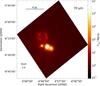 |
Fig. A.1 Monoceros R2 as viewed by Herschel PACS 70 μm. The image is 1.15°×1.3° (16.7×19.1 pc) in size. The diffraction-limited instrumental beam (5.6′′) is shown to the lower left of the image. |
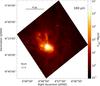 |
Fig. A.2 Monoceros R2 as viewed by Herschel PACS 160 μm. The image is the same area as covered by Fig. A.1. The instrumental beam (11.4′′) is shown to the lower left of the image. |
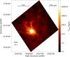 |
Fig. A.3 Monoceros R2 as viewed by Herschel SPIRE 250 μm. The image is the same area as covered by Fig. A.1 (there is a ~ 20′ offset between the SPIRE and PACS images). The instrumental beam (18.1′′) is shown to the lower left of the image. |
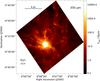 |
Fig. A.4 Monoceros R2 as viewed by Herschel SPIRE 350 μm. Otherwise, the same as for Fig. A.1. The instrumental beam (24.9′′) is shown to the lower left of the image. |
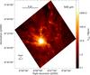 |
Fig. A.5 Monoceros R2 as viewed by Herschel SPIRE 500 μm. Otherwise, the same as for Fig. A.1. The instrumental beam (36.4′′) is shown to the lower left of the image. |
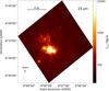 |
Fig. A.6 Monoceros R2 as viewed by MIPS, 24 μm. Otherwise, the same as for Fig. A.1. The instrumental beam (6′′) is shown to the lower left of the image. |
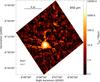 |
Fig. A.7 Monoceros R2 as viewed by SCUBA-2, 850 μm. Otherwise, the same as for Fig. A.1. The instrumental beam (14.1′′) is shown to the lower left of the image. |
Appendix B: The getsources routine
The getsources routine was designed by the SAG-3 consortium to provide the best source extractions possible. It works on multiple wavelengths simultaneously, disentangles sources based on their spatial scales, and comes with a built-in filament-extraction routine (getfilaments). Full details of the routine are given in Men’shchikov et al. (2012), which gives an overview of the routine, and Men’shchikov (2013), which looks in detail at the filament extraction. The routine requires the use of three external libraries: SWarp (Bertin et al. 2002), CFITSIO (Pence 1999), and WCSTools (Mink 2002).
A basic overview of the routine is given here, while more in-depth descriptions of the individual subroutines appear in the following subsections. Initially (monochromatic extraction), getsources is run on each wavelength map separately: the maps are decomposed into their separate spatial scales and cleaned of background noise; sources are detected and measured. This initial extraction is used to find source footprints (the closest ellipse fitting to the source shape), which will be used in a later extraction. The spatial scale maps are now combined across all wavelengths (combined extraction) and sources are detected and measured in the combined maps. Using the source measurements from the previous steps, extended background in the original maps is “flattened” to allow for better detection, and the decomposition, cleaning, combination, detection, and measurement subroutines are run again on these new maps (final extraction).
Preparation
Prior to the start of the routine, all input maps must be prepared using the prepareobs routine (packaged with getsources, but not run as part of the main routine). This resamples all images to the same pixel scale (generally the finest pixel scale is used, which in this paper was 1.4′′, as the run included 70 μm PACS data), and converts the units to MJy/sr. Two copies of each map are made: the “detection” map, which is smoothed very slightly (by about one third of the wavelength’s observational beam), and the “measurement” map, which is left unchanged.
Certain input parameters may also be chosen here; for example, individual maps may be declared “measurement-only”, meaning that the maps are not used for source detection. This can be used to include MIR and SMM maps, without filling the catalogue with sources detected only at these wavelengths.
Decomposition
The detection maps are decomposed into about a hundred separate spatial scale maps. The first scale map follows the equation  , where ℐD is the detection map and
  is a smoothing Gaussian. Larger-scale maps are formed using the smoothed map (
 ) in place of the detection map, and a slightly larger Gaussian. The spatial scales used vary between a few arcseconds and several thousand arcseconds, if the maps allow it. The scale maps are not normalised, and so the original detection map can be recreated by summing them together.
Cleaning
To clean background noise from the spatial scale maps, areas of high emission must first be masked. Initially, all regions higher than 6σ are masked, and then a new value of σ is found from the non-masked area, which is used to mask out regions above the new 6σ (we note that the exact factor of σ used is generally 6, but may differ depending on the scale map’s skewness and kurtosis). This process is iterated until there is no more change in either the mask or the σ value, at which point, every pixel below the new 6σ value (called the noise threshold) is set to zero. Filaments are also extracted in this step, but the exact process is covered in the following subsection.
Filament extraction
During the decomposition phase, objects are split up according to their spatial scales, and so extended objects will be seen only at larger scales, while smaller objects will only be seen at smaller scales. Filaments, however, will be assigned to scales close to their width, rather than their length. Consequently, large regions (the exact value depends on several variables, but is generally several hundred times the beam size, at the smallest scales, and much larger at larger scales) of connected pixels above the σ value in the smaller scale maps are likely to be due to filaments. The filaments are extracted from the images, and sources within them are detected by their small sizes and relatively high intensities, and are removed from the filaments. The filaments are then reconstructed across all spatial scales, and are characterised by the creation of filament skeleton maps.
Combination
The maps for each scale are summed across the wavelengths, creating a set of wavelength-independent spatial scale maps. We note that since the spatial scales have been separated, the wavelengths’ differing resolutions is not an issue. Even so, there will not be much useful data from a scale smaller than about one third of the wavelength’s resolution, and so such scales are not included in the summation. Prior to summation, the maps are normalised, so that weaker sources are not lost (this will not be a problem, since these images are only used for source detection, not for measurement). This section of the routine is not performed in the first (monochromatic) extraction, which is performed on all wavelengths separately.
Detection
To detect sources in the cleaned scale maps, the routine will select multiple values between the maximum intensity and the noise threshold. Pixels above these values are either used to make new sources, or are added to existing (adjacent) ones. The sources are correlated across the scale maps, meaning that each source will have a scale range over which it appears. This is used to distinguish overlapping sources with different spatial scales. At each scale, the source’s “detection significance” is measured; this is equal to the maximum intensity at this scale divided by the noise threshold, and is used to determine how well-detected any source is. Elliptical source footprints are also determined during this stage.
Measurement
Measurement of source properties is performed on the “measurement maps”, which are essentially identical to the input maps. Filaments are removed from the maps, and non-filamentary background is estimated, using the source footprints measured above, and also removed. Sources are deblended by assuming a near-Gaussian profile (with stronger, and thus more realistic, wings; note that the profile is only used to allocate flux by deblending). If the two sources are within one third of a beam size of one another, and their sizes are within a factor of two, they are assumed to be the same source and are thus combined. The properties measured include peak intensity (the value at the peak, in Jy/beam), total flux density (the integral over the whole source, in Jy), and source shape (major and minor axes, and axis angle); the final output is a catalogue listing these values at each wavelength for every source.
Flattening
Before the final extraction, a more robust form of background-subtraction (“flattening”) is employed, in order to account for the problems raised by the variable Galactic backgrounds present in most Herschel images. The first two extractions (monochromatic and combined) were used to find and characterise as many sources as possible, which are then removed from the maps to create clean background maps. This is used to create a map of local (3 × 3 pixels) standard deviation, which is smoothed, first by median filtering, and then by convolution with a Gaussian three times the maximum source size, forming the scaling map, which is used to scale the detection map. This means that highly variable parts of the map will be deemphasised, when compared with the regions with flatter background. We note that this only affects the detection maps; the measurement maps are not changed in any way.
Advantages and disadvantages
The getsources routine works on all wavelengths at once, and at multiple spatial scales at once, which gives it a great advantage over other source finders. It deblends overlapping sources and utilises background flattening to find the best sources possible. Its scale-decomposition allows it to detect sources at both large and small scales, something many other source finders do not do. It is not without disadvantages, most of which stem from the sheer size of the program. For example, many other source finders can run over the five Herschel wavelengths in under an hour, giving one or two output files for each of the five extractions; on the same maps, getsources can run for a week, giving several GB of output. Despite this, the advantages in enhanced detection will generally outweigh the disadvantages in ease (and speed) of use. Discussions of various source finders are given in André et al. (2014) and Rayner (2015). A look at the completeness of getsources in Mon R2 is given in Appendix C.
Appendix C: The completeness of the getsources extraction
In order to test the completeness of the catalogue, the getsources program was run on a field of simulated data based on the original Mon R2 maps, with additional sources superimposed on them. Though there are disadvantages to adding the sources to the original map, as the real sources on the map will add confusion to the output, the alternative (to add simulated sources to a source-free background map) may also have problems caused by artefacts from the source-removal process. The main advantage of using the original map is that the getsources output for the original map alone is already available, and any changes to this output will thus be due to the inserted sources.
The basic technique was based on those of Marsh et al. (2016) and Könyves et al. (2015), albeit with modifications made due to the differences between the regions in question (Mon R2 is at 830 pc, with a very dense central hub, while Taurus and Aquila are at 140 pc and 260 pc respectively, without any regions comparable to the Mon R2 hub). A total of 440 model sources were input into the maps. These included sources modelled as protostars (116), bound (186) and unbound (138) cores, with shapes approximating to 2D Gaussians. The mass range was 0.03–10 M⊙ and temperature and size ranges were chosen to fit with the observed parameter ranges within the region. The fluxes at each wavelength were calculated using the SED in Eq. (4), and their positions on the map were chosen randomly, with protostars and bound sources placed in regions with column densities over 3 × 1021 cm-2, and unbound sources (which do not necessarily trace the highest column densities) placed in regions with a 250 μm intensity over 57 MJy/sr.
The maps used for this procedure were all Herschel (PACS and SPIRE) maps, along with the 850 μm SCUBA-2 map, and the column density map. The 24 μm MIPS map was not included, as this was only used for luminosity calculations. For simplicity, the column density profiles of the sources were added directly into the column density map, rather than having the column density map recreated from the new flux maps.
The getsources routine was run (see Appendix B for details), and the source selection and cataloguing process was run on the output. Model sources were counted as detected when their centres lay within 11.4′′ (the 160 μm beam size) or 30% of the model source size (whichever was larger) of the centre of a detected source. In total, 40% (175 of 440) model sources were detected, about 60% of those above 1 M⊙, but only 20% of those below this value. Consequently, setting a completeness limit of 1 M⊙ would mean that the majority of sources had been detected. The percentage of detected sources against mass is given in Fig. C.1. A detected source also had a ≳75% chance to be assigned the correct source type.
The most likely reason for the low completeness, even at high masses, is the large sizes given to some of these sources by the model core creation routine. Although these were not much larger than the detected sources (the largest model source was 0.35 pc across, compared to 0.30 pc), this did have the consequence that even sources with masses over 20 M⊙ could have densities similar to those of much lower mass, and would thus be much harder to detect. If only sources with the smallest sizes (under 0.03 pc) are considered, the completeness goes up to 80% detection above 1 M⊙, and 100% detection above 4 M⊙, but this is not a full representative sample of all sources in the region.
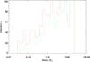 |
Fig. C.1 Completeness of sources. The red line shows the percentage of sources detected by getsources; the green line shows the percentage of sources added to the catalogue. |
A secondary completeness test was applied solely to the central hub, due to its higher confusion and average column density. A further five separate runs placed a total of 212 model sources into the hub (89 protostellar, 70 bound, and 53 unbound), with mass and size ranges equal to those of the original run, and a slight increase in the lower limit of the temperature range, to account for the higher temperatures Other than the area covered, and the number of sources, each of these runs was identical to the original run over the full region. In total, only 33% of model sources with masses above 1 M⊙ (or 20% of all model sources) were detected, half as many proportionally as over the full maps. In addition, a dependence on size was also present, as 79% of detected model sources were under 20′′. The detections against mass for the hub region are shown in Fig. C.2.
Overall, the completeness analysis shows that in the more quiescent parts of Mon R2, more than 60% of sources above 1 M⊙ will be detected robustly. This percentage depends strongly on the size of the object in question, and increases to 90% when dealing strictly with objects under 0.035 pc in size (and 100% of for a mass limit of 4 M⊙), while only 50% of more extended sources are detected (above 1 M⊙). This is seen to an even greater extent within the central hub, where getsources only robustly detects ~30% of sources. As such while it is not feasible to define a mass completeness limit for the larger, less-dense sources, a mass limit of 1 M⊙ for protostars and other compact sources under ~0.035 pc in size is suggested.
Appendix D: Catalogue
Global parameters.
70 μm parameters.
160 μm parameters. As above.
The Mon R2 HOBYS catalogue tables for the first eleven sources are given here (ordered by mass; these are the sources over 10 M⊙). There are ten tables: one containing the source name and position (Table D.1); five containing Herschel getsources output (Tables D.2–D.8); one for each wavelengths of non-Herschel getsources output (in this case, MIPS 24 μm and SCUBA-2 850 μm); one for WISE catalogue fluxes; and one for derived parameters (this table is given in the main body of the paper as Table 4). We note that not all sources have associated WISE sources; only those that do will be included here. A full version of this table, including observed fluxes, and starless cores, is available at the CDS. The full table will contain all robustly detected sources, although with the caveat that the sample is likely incomplete, especially below 1 M⊙. In addition to these tables, the catalogues will contain a set of images for each
source (such as Fig. D.1) showing their appearances at different wavelengths. We note that all fluxes are direct outputs from getsources, without flux-scaling or colour corrections applied.
250 μm parameters. As above.
350 μm parameters. As above.
500 μm parameters. As above.
MIPS 24 μm parameters. As above.
SCUBA-2 850 μm parameters. As above.
WISE fluxes and name.
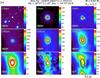 |
Fig. D.1 Images of a probable protostellar core in the Monoceros R2 region at 3.6 μm (IRAC), 24 μm (MIPS), 70 μm, 160 μm (PACS), 250 μm, 350 μm, 500 μm (SPIRE), 850 μm (SCUBA-2) and in the high-resolution column density map (source HOBYS J060711.2 −054721; number 144 in the full catalogue). All images cover the same spatial scale (approximately 100′′ × 100′′, or 0.4 pc × 0.4 pc); this is for consistency across all sources, some of which are much larger than HOBYS J060711.2 −054721. The ellipses show the extent of the source FWHM (assuming a 2d Gaussian shape) as determined by getsources for each individual wavelength. A black ellipse indicates that the detection at this wavelength was either considered reliable (160–850 μm), or was a 70 μm detection used for the SED fit. (The ellipse shown at 3.6 μm is the ellipse measured at the reference wavelength; here 160 μm.) The source mass and angular size at the reference wavelength are given at the upper right of the snapshots. We note that only one set of snapshots is included here; the full catalogue will contain snapshots for all robust sources. The SED of this source is given in Fig. D.2. |
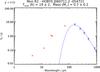 |
Fig. D.2 SED of a probable protostellar core in the Monoceros R2 region. Blue crosses represent reliable data points; red crosses represent short-wavelength data points used only for luminosity calculations (while not present here, some SEDs within the catalogue also show red crosses, albeit with long error-bars, which represent unreliable data points, which are used for SED fitting, but with greatly increased errors). The χ2 value of the fit is given at the upper left of the plot. The snapshots of this source are given in Fig. D.1. We note that the fluxes are those used for the SED calculation, and have thus been modified using flux scaling. |
All Tables
All Figures
|
Fig. 1 Monoceros R2 as viewed by Herschel: PACS 70 μm in blue; PACS 160 μm in green; and SPIRE 250 μm in red. The image is cropped to the approximate overlap between the PACS and SPIRE maps. The black box indicates the central hub, which is shown in more detail in Fig. 2 (due to the large range in brightness, the detailed features of the central hub do not appear clearly in this three-colour image). The positions of the hub itself, and the three surrounding H ii regions are also given. The three maps are given separately (with intensity scales) in Appendix A. |
| In the text | |
|
Fig. 2 Monoceros R2 central hub region as seen at 160 μm. The region viewed is shown as the black box in Fig. 1. The black circle shows the approximate position and extent of the H ii region (Pilleri et al. 2012; Didelon et al. 2015). The sources are from Beckwith et al. (1976), detected between 1.65 μm and 20 μm (the red object is Mon R2 IRS 1). |
| In the text | |
|
Fig. 3 Monoceros R2 high-resolution H2 column density map ( |
| In the text | |
|
Fig. 4 Monoceros R2 dust temperature map. The resolution is as for the 500 μm map (36.4′′). The contours (as for Fig. 3) are at the H2 column densities 7.5 × 1021 cm-2 and 3.5 × 1022 cm-2. |
| In the text | |
|
Fig. 5 Channel map of C18O 2 → 1 emission. Black contours (2.5–7 K km s-1 by 0.5 K km s-1) are overlaid on the Herschel column density map in colour (Fig. 3). Filaments identified in the C18O and in the Herschel map are classified F1–F8 and traced in grey. |
| In the text | |
|
Fig. 6 Colour map of the Herschel column density (Fig. 3), overlaid with polygons (F1–F8) indicating the areas over which the filament properties (average column density, density, temperature, and total mass) were determined. The white contours show the filaments identified by getsources in the column density map. |
| In the text | |
|
Fig. 7 Monoceros R2 sources, on the 250 μm flux map (Fig. A.3). The getfilaments map is overlaid as black contours (strictly, these are the filaments detected on the column density map at scales below 72′′). The contours are those from Fig. 3 (H2 column densities 3 × 1021 cm-2 and 1.5 × 1022 cm-2). A zoom-in of the region in the red box (the central hub) is shown in Fig. 8. The points are protostars (blue), bound cores (green), and unbound clumps (red); see text for details. |
| In the text | |
|
Fig. 8 Zoom in on the central hub region of Fig. 7. The contour shows the filaments as detected by getsources on the column density map. |
| In the text | |
|
Fig. 9 Bolometric luminosity-mass plot for robust sources in Mon R2. The coloured symbols represent protostars (blue diamonds), bound cores (green squares), and unbound clumps (red triangles). Filled shapes are sources within the central hub. The black lines represent evolutionary tracks for protostars with final protostellar masses of 0.6 M⊙, 2 M⊙, 8 M⊙, and 20 M⊙ (described in Sect. 7). |
| In the text | |
|
Fig. 10 Mon R2 plot of mass against reference size (full width at half maximum at either 160 μm or 250 μm; defined in Sect. 6). As for Fig. 9. The two lines of protostellar (blue) sources are at half the 160 μm and 250 μm beam sizes (5.7′′ and 9.1′′, respectively, corresponding to sizes 0.023 pc and 0.037 pc), which were taken as the minimum source sizes (see Sect. 6 for more details). |
| In the text | |
|
Fig. A.1 Monoceros R2 as viewed by Herschel PACS 70 μm. The image is 1.15°×1.3° (16.7×19.1 pc) in size. The diffraction-limited instrumental beam (5.6′′) is shown to the lower left of the image. |
| In the text | |
|
Fig. A.2 Monoceros R2 as viewed by Herschel PACS 160 μm. The image is the same area as covered by Fig. A.1. The instrumental beam (11.4′′) is shown to the lower left of the image. |
| In the text | |
|
Fig. A.3 Monoceros R2 as viewed by Herschel SPIRE 250 μm. The image is the same area as covered by Fig. A.1 (there is a ~ 20′ offset between the SPIRE and PACS images). The instrumental beam (18.1′′) is shown to the lower left of the image. |
| In the text | |
|
Fig. A.4 Monoceros R2 as viewed by Herschel SPIRE 350 μm. Otherwise, the same as for Fig. A.1. The instrumental beam (24.9′′) is shown to the lower left of the image. |
| In the text | |
|
Fig. A.5 Monoceros R2 as viewed by Herschel SPIRE 500 μm. Otherwise, the same as for Fig. A.1. The instrumental beam (36.4′′) is shown to the lower left of the image. |
| In the text | |
|
Fig. A.6 Monoceros R2 as viewed by MIPS, 24 μm. Otherwise, the same as for Fig. A.1. The instrumental beam (6′′) is shown to the lower left of the image. |
| In the text | |
|
Fig. A.7 Monoceros R2 as viewed by SCUBA-2, 850 μm. Otherwise, the same as for Fig. A.1. The instrumental beam (14.1′′) is shown to the lower left of the image. |
| In the text | |
|
Fig. C.1 Completeness of sources. The red line shows the percentage of sources detected by getsources; the green line shows the percentage of sources added to the catalogue. |
| In the text | |
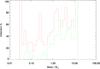 |
Fig. C.2 Completeness of sources in the hub region; otherwise, as for Fig. C.1. |
| In the text | |
|
Fig. D.1 Images of a probable protostellar core in the Monoceros R2 region at 3.6 μm (IRAC), 24 μm (MIPS), 70 μm, 160 μm (PACS), 250 μm, 350 μm, 500 μm (SPIRE), 850 μm (SCUBA-2) and in the high-resolution column density map (source HOBYS J060711.2 −054721; number 144 in the full catalogue). All images cover the same spatial scale (approximately 100′′ × 100′′, or 0.4 pc × 0.4 pc); this is for consistency across all sources, some of which are much larger than HOBYS J060711.2 −054721. The ellipses show the extent of the source FWHM (assuming a 2d Gaussian shape) as determined by getsources for each individual wavelength. A black ellipse indicates that the detection at this wavelength was either considered reliable (160–850 μm), or was a 70 μm detection used for the SED fit. (The ellipse shown at 3.6 μm is the ellipse measured at the reference wavelength; here 160 μm.) The source mass and angular size at the reference wavelength are given at the upper right of the snapshots. We note that only one set of snapshots is included here; the full catalogue will contain snapshots for all robust sources. The SED of this source is given in Fig. D.2. |
| In the text | |
|
Fig. D.2 SED of a probable protostellar core in the Monoceros R2 region. Blue crosses represent reliable data points; red crosses represent short-wavelength data points used only for luminosity calculations (while not present here, some SEDs within the catalogue also show red crosses, albeit with long error-bars, which represent unreliable data points, which are used for SED fitting, but with greatly increased errors). The χ2 value of the fit is given at the upper left of the plot. The snapshots of this source are given in Fig. D.1. We note that the fluxes are those used for the SED calculation, and have thus been modified using flux scaling. |
| In the text | |
Current usage metrics show cumulative count of Article Views (full-text article views including HTML views, PDF and ePub downloads, according to the available data) and Abstracts Views on Vision4Press platform.
Data correspond to usage on the plateform after 2015. The current usage metrics is available 48-96 hours after online publication and is updated daily on week days.
Initial download of the metrics may take a while.