| Issue |
A&A
Volume 606, October 2017
|
|
|---|---|---|
| Article Number | A99 | |
| Number of page(s) | 26 | |
| Section | Extragalactic astronomy | |
| DOI | https://doi.org/10.1051/0004-6361/201731000 | |
| Published online | 20 October 2017 | |
Physical conditions of the molecular gas in metal-poor galaxies⋆
1 INAF–Osservatorio Astrofisico di Arcetri, Largo E. Fermi, 5, 50125 Firenze, Italy
e-mail: This email address is being protected from spambots. You need JavaScript enabled to view it.
2 Max-Planck-Institut für Radioastronomie, Auf dem Hügel 69, 53121 Bonn, Germany
3 Astronomy Department, King Abdulaziz University, PO Box 80203, Jeddah, Saudia Arabia
4 Observatoire de Paris, LERMA, Collège de France, CNRS, PSL, Sorbonne University UPMC, 75014 Paris, France
5 Observatorio Astronómico Nacional (OAN)-Observatorio de Madrid, Alfonso XII, 3, 28014 Madrid, Spain
6 Max-Planck-Institut für extraterrestrische Physik, Giessenbachstrasse 1, 85748 Garching, Germany
7 Cavendish Laboratory, University of Cambridge, 19 J.J. Thomson Avenue, Cambridge CB3 0HE, UK
8 ESO, Karl Schwarzschild str. 2, 85748 Garching bei München, Germany
9 Vittja 64, 74793 Alunda, Sweden
Received: 18 April 2017
Accepted: 8 August 2017
Abstract
Studying the molecular component of the interstellar medium (ISM) in metal-poor galaxies has been challenging because of the faintness of carbon monoxide emission, the most common proxy of H2. Here we present new detections of molecular gas at low metallicities, and assess the physical conditions in the gas through various CO transitions for 8 galaxies. For one, NGC 1140 (Z/Z⊙ ~ 0.3), two detections of 13CO isotopologues and atomic carbon, [Ci](1–0) and an upper limit for HCN(1–0) are also reported. After correcting to a common beam size, we compared 12CO(2–1)/12CO(1–0) (R21) and 12CO(3–2)/12CO(1–0) (R31) line ratios of our sample with galaxies from the literature and find that only NGC 1140 shows extreme values (R21 ~ R31 ~ 2). Fitting physical models to the 12CO and 13CO emission in NGC 1140 suggests that the molecular gas is cool (kinetic temperature Tkin ≲ 20 K), dense (H2 volume density nH2 ≳ 106 cm-3), with moderate CO column density (NCO ~ 1016 cm-2) and low filling factor. Surprisingly, the [12CO]/[13CO] abundance ratio in NGC 1140 is very low (~8−20), lower even than the value of 24 found in the Galactic Center. The young age of the starburst in NGC 1140 precludes 13CO enrichment from evolved intermediate-mass stars; instead we attribute the low ratio to charge-exchange reactions and fractionation, because of the enhanced efficiency of these processes in cool gas at moderate column densities. Fitting physical models to 12CO and [Ci](1–0) emission in NGC 1140 gives an unusually low [12CO]/[12C] abundance ratio, suggesting that in this galaxy atomic carbon is at least 10 times more abundant than 12CO.
Key words: galaxies: starburst / galaxies: dwarf / galaxies: star formation / galaxies: ISM / ISM: molecules / radio lines: ISM
Based on observations carried out with the IRAM 30 m and the Atacama Pathfinder Experiment (APEX). IRAM is supported by the INSU/CNRS (France), MPG (Germany), and IGN (Spain), and APEX is a collaboration between the Max-Planck-Institut fur Radioastronomie, the European Southern Observatory, and the Onsala Space Observatory.
© ESO, 2017
1. Introduction
Physical conditions in the molecular component of the interstellar medium (ISM) of metal-poor galaxies are difficult to measure. The main obstacle is the faintness at low metallicities of the common proxy of H2, carbon monoxide emission (Sage et al. 1992; Taylor et al. 1998; Gondhalekar et al. 1998; Barone et al. 2000; Leroy et al. 2005, 2007; Buyle et al. 2006; Schruba et al. 2012; Cormier et al. 2014). While the proximity of Local Group galaxies facilitates studies of molecular gas (e.g., Cohen et al. 1988; Rubio et al. 1993, 2015; Fukui et al. 1999; Israel et al. 2003; Bolatto et al. 2008; Pineda et al. 2012; Elmegreen et al. 2013; Paron et al. 2014; Shi et al. 2015; Paron et al. 2016; Shi et al. 2016; Schruba et al. 2017), beyond the Local Group, CO detections in low-metallicity galaxies are arduous (e.g., Schruba et al. 2012; Cormier et al. 2014), and few in number. In a previous paper (Hunt et al. 2015, hereafter Paper I), we reported 12CO(1–0) detections in 8 metal-poor galaxies outside the Local Group with metallicities ranging from 12 + log(O/H) ~ 7.7 to 8.4, or equivalently 0.1 Z⊙ to 0.5 Z⊙1. This more than doubles the previous number of such detections, and sets the stage for a more detailed study of the physical conditions in molecular gas in a metal-poor ISM.
Parameters for observed galaxies.
In this paper, we present observations of 12CO(2–1) and 12CO(3–2) for some of the galaxies in Paper I, and for one of them, NGC 1140, also 12CO(4–3), 13CO(1–0), 13CO(2–1), and [Ci](1–0) detections, as well as upper limits for other molecular transitions including HCN(1-0). In Sect. 2, we briefly discuss the sample, and in Sect. 3, describe the observations and data reduction. Section 4 presents our approach for correcting the observed temperatures and fluxes for the different beam sizes. Section 5 analyzes the observed line ratios from an empirical point of view, comparing them with other metal-rich samples, and Sect. 6 discusses dense-gas tracers. Physical models of the line emission of NGC 1140 are presented in Sect. 7, in order to infer H2 volume density, nH2, kinetic temperature, Tkin, CO column density, NCO, and the 12CO/13CO as well as the [Ci]/12CO abundance ratios. More limited models are computed for the other galaxies with fewer multiple transitions. We discuss the results in Sect. 8, and give our conclusions in Sect. 9.
2. The targets
A complete description of source selection and the individual galaxies is given in Paper I. Here we briefly outline the main selection criteria and general characteristics of our targets.
The majority of the galaxies in the observing sample already had H2 detections, either of the ro-vibrational transitions at 2 μm or the rotational transitions in the mid-infrared with Spitzer/IRS (Hunt et al. 2010). Additional galaxies were included with previous CO observations lacking a clear detection. Stellar masses, estimated from 3.6 μm luminosities after the subtraction of nebular emission, range from ~108 to 1010 M⊙ (UM 448 is more massive than this, and is the clear result of an interaction with another galaxy, see Paper I for more details). The relatively high specific star-formation rates (ratio of SFR and stellar mass, SFR/Mstar = sSFR) of the sample make them starburst galaxies (sSFR ≳ 10-10 yr-1). They are also gas rich, with gas-mass fractions (relative to total baryonic mass) as high as ~0.8.
3. The observations
We have observed 12CO(1–0) and 12CO(2–1) in our sample galaxies over a three-year period from 2008 to 2010 with the IRAM 30-m telescope (Pico Veleta, Spain). The measurements of 12CO(3–2) and for a few galaxies also of 12CO(2–1) were acquired with the APEX 12-m telescope (Chile)2. NGC 1140 was singled out for a more intense observing campaign in which we observed 13CO(1–0), HCN(1–0), other 3-mm transitions, and 13CO(2–1) at the 30 m; 12CO(4–3) and [Ci](1–0) measurements were obtained with APEX. The 12CO(1–0) observations of this sample were presented in Paper I. Table 1 reports selected observational parameters for the sample galaxies. Our single-dish observations sample fairly large regions within each galaxy, ranging from 420 pc for the smallest beam in the closest galaxy (12CO(2–1), NGC 1156) to 8.5 kpc for the largest beam in the most distant one (12CO(1–0), UM 448).
3.1. IRAM
We observed eight galaxies at the 30 m in 12CO(1–0) and 12CO(2–1), first with the older ABCD receivers (proposals 036-08, 227-09), then with the Eight Mixer Receiver (EMIR, proposal 097-10) using the Wideband Line Multiple Autocorrelator (WILMA) backend. Earlier spectra were acquired at an intrinsic resolution of 4 MHz, while later ones using EMIR at 2 MHz. For NGC 1140, the EMIR E090 receiver was tuned to an intermediate frequency, ~113 GHz, in order to cover other 3 mm transitions simultaneously together with 12CO(1–0) in the lower-inner sideband in two polarizations. We adopted wobbler switching with a throw of 90′′, and used the standard intensity calibration with two absorbers at different temperatures. Pointing was checked every hour or two on nearby planets or bright quasars, and focus tests were performed every 4 h during the night and every 3 h during the day. Typical pointing errors were ≲2′′, and never exceeded ~3′′.
With the EMIR setup for NGC 1140, we were able to also observe additional transitions, including 13CO(1–0), 13CO(2–1), C18O(1–0), and the dense-gas tracers HCN(1–0), CN(1–0), and CS(2–1).
CO emission line parameters for CGCG 007−025, Mrk 996, NGC 1156, and NGC 3353.
CO emission line parameters for NGC 7077, UM 448 and UM 462
Emission line parameters for NGC 1140.
3σ upper limits of undetected emission lines for II Zw 40 and SBS 0335−052.
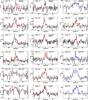 |
Fig. 1 Various 12CO transitions for Mrk 996, NGC 3353, NGC 7077, NGC 1156, and UM 448. Top row: 12CO(1–0), 12CO(2–1) (IRAM), and 12CO(2–1) (APEX) for Mrk 996; second row: 12CO(1–0) for NGC 3353 (Haro 3) for three pointings ([0, 0], [0, +10′′], [−6′′, −9′′]); third row: 12CO(2–1) for NGC 3353 (Haro 3) for three pointings; fourth row: 12CO(1–0), 12CO(2–1) (IRAM), and 12CO(3–2) (APEX) for NGC 7077 (Mrk 900); fifth row: 12CO(1–0) for NGC 1156 and UM 448, and 12CO(2–1) (APEX) for UM 448; bottom row: 12CO(2–1) (IRAM) for NGC 1156 and UM 448 and 12CO(3–2) (APEX) for UM 448. The baselines are shown as a horizontal solid line, together with the multiple-component Gaussian fits as described in Sect. 3.3. The vertical axes are in |
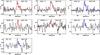 |
Fig. 2 12CO, 13CO, and [Ci](1–0) transitions for NGC 1140. Top row: 12CO(1–0), 12CO(2–1) (IRAM), and 12CO(3–2) (APEX); second row: 13CO(1–0), 13CO(2–1) (IRAM), and 12CO(4–3) (APEX); third row: [Ci](1–0) (APEX). As in Fig. 1, the baselines are shown as a horizontal solid line, together with the multiple-component Gaussian fits as described in Sect. 3.3. The vertical axes are in |
3.2. APEX
The 12CO(3–2) observations of six of our targets were performed with the Swedish Heterodyne Facility Instrument (SHeFI) at the 12-m Atacama Pathfinder Experiment telescope (APEX). The observations were acquired over three observing periods from 2008 to 2010 as part of the proposals 082.B-0795A, 085.F-9320A, and 087.F-9316A. 12CO(2–1) measurements were also obtained for some sources, as reported in Tables 2, 3, and 5. We used the “standard” receiver+backend configurations, APEX-1 (HET230+FTTS1) at 230 GHz and APEX-2 (HET345+FTTS1) at 345 GHz, with an intrinsic resolution of 0.12 MHz at both frequencies. The sources were small enough to be observed in one pointing with wobbler switching (in ON/OFF mode); pointing was checked every 2 h, and calibrations were performed every 10 min. Pointing accuracy was typically ≲2′′. System temperatures for the 12CO(3–2) (12CO(2–1)) observations ranged from ~180 K to 670 K (~160 K to 270 K) with precipitable water vapor from 0.2 mm to 1.1 mm (1.2 mm to 3 mm).
Only NGC 1140 was observed in the 12CO(4–3) and [Ci](1–0) transitions (Period 82), following the same observing protocols as for the lower frequencies but with APEX-3 (HET460+FTTS1) at 460 GHz (intrinsic resolution 0.98 MHz). System temperatures for these higher frequency observations ranged from ~380 K to 740 K (~370 K to 550 K) for [Ci](1–0) (12CO(4–3)). Water vapor columns ranged from 0.2 mm to 0.6 mm for [Ci], and from 0.3 mm to 0.4 mm for 12CO(4–3).
3.3. Data reduction
We adopted the GILDAS/CLASS data reduction package3 to obtain averaged spectra for all transitions. To remove the baseline from each spectrum, a polynomial was fitted to the line-free regions of each scan (defined a priori) and subtracted; the scans were thereafter Hanning smoothed and averaged, and a constant baseline subtracted. We measured the peak intensities, central velocities, full width half-maximum (FWHM) and velocity-integrated fluxes of the detected lines by fitting Gaussian profiles to the data. In most cases, there is significant velocity structure in the emission, so we fit the line profiles to multiple Gaussians. In these cases we use the sum of the integrated line intensities from the multiple Gaussian fits in the analysis.
Antenna temperatures ( ) have been converted to main-beam brightness temperatures (Tmb) by dividing the antenna temperatures by η ≡ Beff/Feff, where Beff and Feff are the beam and forward hemisphere efficiencies, respectively (i.e., Tmb = /η). To convert the measured 12CO(1–0) antenna temperatures, [Tmb (K)] to fluxes [S (Jy)], we used the standard conversion factors for both telescopes. The 12CO(1–0), 12CO(2–1), and 12CO(3–2) line profiles for the galaxies in which CO was detected are shown in Fig. 1, together with the Gaussian fits obtained using the GILDAS/CLASS package as described above and reported in Tables 2–4. The upper limits for II Zw 40 and SBS 0335−052 are given in Table 5. Limits for non-detections are 3σ, taking the width of three contiguous velocity channels and the rms noise in line-free regions of the spectrum.
For the total flux in each transition, we have included the different velocity components in each galaxy into a global, spectrally-integrated sum. While some of the spectra show slightly different profiles in the different transitions, the signal-to-noise (S/N) is insufficient to allow an analysis of the separate components. Although a few of the individual components may be too narrow to be significant (because their width is smaller than three velocity channels, e.g., Mrk 996, NGC 3353, NGC 1140, see Figs. 1, 2), we have checked that the total intensities are robust to the details of the fitting by repeating the fits with different numbers of components. Some of the measured values in the tables differ slightly from those given in Paper I; this is because we have redone the data reduction for all transitions in order to render the results as consistent as possible. The main difference is the newer version of CLASS used here that seems to give integrated fluxes which can differ by a few percent (but within the error limits) with respect to those in Paper I (performed with an older version of CLASS).
In Paper I, for the galaxies with the largest apparent sizes, to estimate total 12CO(1–0) flux beyond even the largest beam we applied aperture corrections. Here they are not adopted because we prefer to correct the observations to a common beam size, rather than also extrapolating to an uncertain total flux.
3.4. Comparison with previous observations
A detailed comparison of our 12CO(1–0) measured intensities relative to previous work is given in Paper I. Here we compare only the higher-J CO transitions with published literature values. Sage et al. (1992) observed II Zw 40, NGC 3353 (Haro 3), NGC 7077, and UM 462 in 12CO(2–1), and securely detected only the first three. Like the 12CO(1–0) measurements, their results from the IRAM 30 m for 12CO(2–1) in NGC 3353 are in good agreement with the line parameters deduced from our central pointing. For NGC 7077, our 12CO(2–1) flux of 1.06 K km s-1 is ≳50% larger than the value of 0.68 K km s-1 reported by Sage et al. (1992); given the similar uncertainties, it is difficult to understand the discrepancy, especially since our 12CO(1–0) flux is smaller than theirs by ~30%. Our 12CO(2–1) non-detection for UM 462 is consistent with the non-detection by Sage et al. (1992), while our upper limit is smaller. Instead, our non-detection with APEX of 12CO(2–1) in II Zw 40 is inconsistent with Sage et al. (1992); at the flux level found by them, we should have detected this galaxy, as our 3σ upper limit is several times smaller.
NGC 1140 and II Zw 40 were also observed previously in 12CO(2–1) with the IRAM 30 m by Albrecht et al. (2004). Although the 2–1/1–0 line ratios for NGC 1140 are similar, they find ~40–60% larger intensities in both lines. The line intensity they report for the IRAM 30-m spectrum of II Zw 40 (UGCA 116) is larger than our APEX upper limit, although less than half of the 30 m detection reported by Sage et al. (1992). The peak 12CO(3–2) temperatures observed with ALMA in the main knots in II Zw 40 by Kepley et al. (2016) exceed those of our upper limits; but beam dilution is probably playing an important role since the ALMA beam is ~0.̋5 compared to the APEX beam of ~18′′.
One of our targets, NGC 7077, was observed by Mao et al. (2010). The ratio of 12CO(3–2) to 12CO(1–0) we find for this galaxy of 1.1 is in excellent agreement with their study.
In conclusion, there is no clear systematic difference between our results and previous work. Nevertheless, the formal uncertainties given in Tables 2–5 should probably be considered as lower limits to the true uncertainties.
4. Correction to a common beam size
The main difficulty in the interpretation of line ratios from single-dish observations is the correction for different beam sizes. The physical models we discuss in Sect. 7 rely on brightness temperatures TB within a common beam size, while we observe main-beam brightness temperatures, Tmb, within different beams. To correct for this, we have pursued two independent approaches:
-
1.
Used maps of the cool dust emission (~160 μm) to scale the different transitions to a common beam size of 22′′, with the underlying assumption that the molecular emission is distributed like the cool dust. The PACS 160 μm maps are particularly well suited to such an endeavor because their intrinsic FWHM is ~11′′, similar to the smallest beam size in our observations (12CO(2–1), 10.̋7).
-
2.
Assumed that the molecular emission follows a Gaussian distribution with a FWHM size to be determined by letting it vary in the fit to the line intensities. This can be done in a robust way only for NGC 1140 where we have a sufficient number of line intensities to constrain the fit.
Observations at high spatial resolution (≲2 pc) of metal-poor galaxies in the Local Group suggest that the CO clouds are more concentrated than the dust emission (e.g., Rubio et al. 2015; Schruba et al. 2017); if this were true also on the spatial scales probed by our observations (≳500 times larger), then our assumption that the gas follows the dust would be incorrect. Thus, analyzing beam correction factors under the assumption of a Gaussian distribution enables an independent assessment of the validity of the inferred beam corrections.
Appendix A describes the formulation of the correction to a common beam size assuming that the molecular emission follows the dust. In brief, we have established that the distribution of the cool dust emission in our targets is well described by an exponential distribution by extracting azimuthally-averaged radial brightness profiles; they are all well fit by an exponential. Moreover, for our targets, 160 μm emission is longward of the spectral energy distribution peak, thus tracing as well as possible the cool dust component. We have checked that free-free emission is unimportant at 160 μm by inferring its amplitude from the observed SFR (Paper I); for all galaxies for which we have dust images, the expected free-free component is ≲0.1% of the observed emission.
We performed aperture photometry to obtain growth curves, in order to approximate the cumulative flux distribution we expect for the molecular gas in the different beams. Finally, we have followed an analytical approach to fit the growth curves, in order to derive the corrections to the expected flux in different apertures. Table A.1 gives the multiplicative correction factors, and the corrected velocity-integrated Tmb values that we will use throughout the paper unless otherwise noted; corrected intensities are also given in the last three columns in Tables 2–4. While high-J CO emission may be more compact than the gas traced by the lower-J lines, the different radial distributions are expected to be a second-order effect; our proposed correction provides the bulk of the “first-order” correction.
Appendix B discusses the form of the growth curves for a Gaussian source distribution. The main difficulty with applying the Gaussian assumption is the unknown source size; while the source extent can be measured from the analysis of the dust emission, there is no similar way to assess the size of a Gaussian distribution. Thus, when we estimate the physical conditions in the molecular gas by fitting the line intensities (for NGC 1140, the only source for which this is possible), we use the fitting procedure itself to define the source size. The expectation is that because of the similarity of some of the beams in our observations (e.g., 12CO(2–1) with IRAM, 12CO(4–3) with APEX), the fit will be sensitive to the beam correction. This turns out to be the case as will be described in Sect. 7.3.
Mrk 996 shows a markedly broader 12CO(2–1) profile in the larger (27′′) APEX beam, relative to the IRAM one (11′′). This could be an illustration of the spatial extension of the 12CO(2–1) emitting gas, because of the broader velocity range in the bigger beam; on the other hand, the APEX spectrum is rather noisy, so its reliability is uncertain. Nevertheless, the optical diameter of Mrk 996 is 36′′ so it is conceivable that there is more CO emission in the larger APEX beam. UM 448 was also observed in 12CO(2–1) with both the 30 m and APEX, but in this galaxy the shape and breadth of the two profiles are more similar, possibly because the galaxy is smaller, 24′′ in diameter.
5. Empirical line ratios
Before describing our models of the molecular gas, here we discuss three commonly used diagnostic ratios, 12CO(2–1)/12CO(1–0), 12CO(3–2)/12CO(1–0), and [Ci](1–0)/12CO(1–0). These ratios are calculated using velocity-integrated main-beam temperature,  (see Tables 2–4).
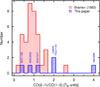 |
Fig. 3 Histogram of observed 12CO(2–1)/12CO(1–0) line ratios for our targets corrected for beam dilution as described in Sect. 4. Because of the larger beam, for Mrk 996 and UM 448, we show the APEX 12CO(2–1) measurements rather than the ones from IRAM. Also plotted are the line ratios corrected for beam dilution of a large sample of spiral galaxies observed by Braine & Combes (1992). |
5.1. CO(2–1)/CO(1–0)
The 12CO(2–1) transition traces slightly warmer (upper level equivalent temperature ~17 K) and denser (critical density ~104 cm-3) gas than the 1−0 transition. In most galaxies, CO emitting gas is optically thick and the observed CO(2–1)/CO(1–0) ratios are ≲1 (e.g., Braine & Combes 1992). Figure 3 shows the distribution of the 12CO(2–1)/12CO(1–0) line temperature ratios (R21) of our low-metallicity targets together with R21 ratios (corrected for beam dilution) of spiral galaxies from Braine & Combes (1992). In Fig. 3, our data are corrected to a common beam size using the exponential approach described in Sect. 4 and in Appendix A.
Even after correction for beam dilution, half of our targets have R21 ≳ 2, higher than most of the normal spirals studied by Braine & Combes (1992). Braine & Combes (1992) found an extremely high ratio for another sub-solar metallicity starburst, NGC 3310 with R21 ~ 2.6; however Zhu et al. (2009) were unable to confirm this, finding a somewhat lower ratio (R21 ~ 1.5), after convolving the observations to a common beam size through their maps.
Although it is tempting to claim that the high R21 observed in some of these dwarf galaxies is due to optically thin gas, the R21 values are somewhat uncertain because of the beam correction. First, the ratios are dependent on the kind of correction applied. The corrections are sensitive both to the source distribution (exponential versus Gaussian) and to the source size (exponential scale length versus Gaussian FWHM); since we have no way of accurately determining a Gaussian FWHM, we cannot assess how much the R21 values would change under another assumption for source distribution. Second, if we use the IRAM 12CO(2–1) observations (with a smaller beam) for Mrk 996 and UM 448, we obtain beam-corrected R21 ~ 0.6 for Mrk 996, and R21 ~ 1.2 for UM 448. Thus the high R21 values are not altogether robust. The only galaxy in our sample for which we are fairly certain that the true R21 value is ≳2 is NGC 1140. The interpretation of R21 for this galaxy will be discussed in Sect. 7.3 where we present physical models for the molecular gas.
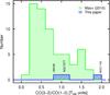 |
Fig. 4 Histogram of observed 12CO(3–2)/12CO(1–0) line ratios for our targets. Also shown are the line ratios for a large sample of galaxies observed by Mao et al. (2010). Neither set of observations has been corrected for beam dilution; see Sect. 5.2 for more discussion. |
5.2. CO(3–2)/CO(1–0)
Figure 4 shows the distribution of the ratio of 12CO(3–2)/12CO(1–0) (R31 in Tmb units) for the three sources in our sample with 12CO(3–2) detections, compared to the large sample of Mao et al. (2010). Unlike for the 12CO(2–1)/12CO(1–0) ratio observed with the IRAM 30 m, the APEX beam is ~18′′, similar to the IRAM 30-m beam of ~22′′ for the 1–0 line; the Mao et al. (2010) observations were obtained with the Heinrich Hertz Telescope with a 12CO(3–2) beam of ~22′′. Thus, we have not applied any correction for beam dilution; the R31 values shown in Fig. 4 should be relatively impervious to beam corrections, but rather representative of the beam-averaged physical conditions in the molecular gas.
Of the three galaxies in our sample with 12CO(3–2) detections (Mrk 996 was observed but not detected, R31 < 0.7), NGC 1140 shows the largest ratio (R31 = 2.00 ± 0.45; with the exponential beam correction R31 = 1.72 ± 0.39), roughly equivalent to that found for NGC 3310 (R31 = 1.9±0.52) by Mao et al. (2010). Such a ratio exceeds typical values in luminous infrared galaxies (LIRGs) and those expected in the Orion “hot spots” (Papadopoulos et al. 2012). R31 has been historically taken as an indicator of H2 density (e.g., Mauersberger et al. 1999), and high R31 is possibly indicative of somewhat excited, optically thin, gas, although shocks and cool foreground absorbing layers are also possible causes (e.g., Oka et al. 2007). We shall explore this point further with physical radiative transfer models in Sect. 7.2.
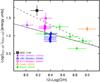 |
Fig. 5 Beam-corrected [Ci]/12CO(1–0) line ratios for NGC 1140 and galaxies from the literature plotted against oxygen abundance 12 + log(O/H). The solid line corresponds to the data regression by Bolatto et al. (2000a), and the dashed one to the PDR model by Bolatto et al. (1999). Beam dilution has been corrected for as described in Sect. 4. |
5.3. CI(1–0)/CO(1–0)
Together with CO and Cii (at 158 μm), the atomic carbon line [Ci](1–0) is an important coolant of the ISM (e.g., Bolatto et al. 1999; Gerin & Phillips 2000; Bolatto et al. 2000a,b,c; Israel & Baas 2002; Papadopoulos et al. 2004; Bayet et al. 2006; Israel 2009). Despite the difficulty of observation from the ground (the  [Ci] transition lies at 609 μm), the potential of atomic carbon to trace molecular gas was recognized early on. Photo-Dissociation Regions (PDRs) are thought to be larger at low metallicity, because of the decreased attenuation of the UV field through the lower dust content (e.g., Lequeux et al. 1994; Bolatto et al. 1999). The brighter UV field in low AV environments tends to change the structure of PDRs, enlarging the region where atomic and ionized carbon dominate, and diminishing the region where H2 is associated with CO emission (e.g., Bolatto et al. 2013). The spatial distributions of [Ci] and CO gas are similar in regions within the Milky Way (e.g., Kramer et al. 2004; Zhang et al. 2007), the Small Magellanic Cloud (SMC, Requena-Torres et al. 2016), and other galaxies (e.g., Israel & Baas 2003; Krips et al. 2016), so [Ci] seems to be tracing molecular gas. This is especially important in low-metallicity environments or cosmic-ray dominated regions where CO emission is suppressed (e.g., Hopkins et al. 2013; Bisbas et al. 2015, 2017), or in high-redshift galaxies where [Ci] observations are facilitated (e.g., Walter et al. 2011).
We have obtained a [Ci](1–0) measurement of one of our targets, NGC 1140, as shown in Fig. 5 where we plot the [Ci]/12CO(1–0) ratio (in energy units) together with similar measurements from the literature (Bolatto et al. 2000a,b,c; Israel & Baas 2002; Bayet et al. 2006). We have applied the correction for beam dilution as described in Sect. 4 and Appendix A. The regression lines are taken from the PDR model by Bolatto et al. (1999, dashed line), and the best fit to their data (Bolatto et al. 2000a). Despite the paucity of data, the trend of enhanced [Ci](1–0)/12CO(1–0) with decreasing O/H is evident.
The expected metallicity-dependent behavior of [Ci](1–0) in PDR environments has been modeled by various groups (e.g., Papadopoulos et al. 2004) who confirm that the abundance of [Ci] dominates that of CO for large regions within a low-metallicity cloud (AV ≳ 2). Glover & Clark (2016) present more recent simulations of [Ci](1–0) emission relative to 12CO(1–0) as a function of metallicity. Our (beam-corrected) [Ci](1–0)/12CO(1–0) velocity-integrated temperature ratio for NGC 1140 of 0.65 (see Table 4) is more than a factor of two higher than their predictions for the highest PDR illumination they model (G0 = 100 in units of the interstellar radiation radiation field by Draine 1978), and the disagreement increases for less intense fields.
The [Ci]/12CO(1–0) ratio tends to decrease with increasing PDR density; the observed ratio for NGC 1140 is higher than the predictions of (solar metallicity) PDR models with volume number densities n0 ~ 104 cm-3 and G0 ~ 104 (Hollenbach et al. 1991). The observed [Ci](1–0)/13CO(2–1) for NGC 1140 is a factor of 4−5 higher than the PDR predictions (for solar, and twice solar metallicities) by Meijerink et al. (2007), for volume number densities n0 ≳ 104 cm-3 and G0 ~ 105. However, they assume [12CO/13CO] = 40; a lower isotopic ratio (see Sect. 7.3) or a lower metallicity would reduce the disagreement. In Sect. 7.3, we explore physical models of the gas in NGC 1140 and derive relative abundances of atomic carbon and CO.
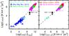 |
Fig. 6 HCN luminosity plotted against FIR luminosity, LFIR (left panel) and CO(1–0) luminosity, |
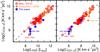 |
Fig. 7 CO(3-2) luminosity, |
6. Dense-gas tracers
The relatively high critical densities of 12CO(3–2) and HCN(1–0) (ncrit ~ 104−105 cm-3) make these transitions good tracers of dense gas, which are possibly better correlated with SFR than the lowest-J CO lines (Gao & Solomon 2004; Narayanan et al. 2005, 2008; García-Burillo et al. 2012; Lada et al. 2012; Hopkins et al. 2013; Greve et al. 2014). Given the relatively high sSFRs of our targets (sSFR ≳ 10-10 yr-1, see Paper I), here we examine luminosity correlations of 12CO(3–2) and HCN(1–0) for these metal-poor galaxies and compare them with more massive metal-rich ones.
Figure 6 shows HCN luminosity plotted against FIR luminosity, LFIR (left panel) and CO(1–0) luminosity,  (right). The only galaxy for which we have HCN(1–0) observations is NGC 11404; also shown in Fig. 6 are luminous (and ultraluminous) infrared galaxies from Gao & Solomon (2004), Graciá-Carpio et al. (2008), García-Burillo et al. (2012), together with regions within M 33 (Buchbender et al. 2013) and the Milky Way (MW, Wu et al. 2010); a luminous irregular galaxy, He 2–10, is also plotted (Santangelo et al. 2009). The dashed lines show a robust regression5 performed on all galaxies excepting He 2–10 and NGC 1140; the power-law index of the
  –LFIR correlation is 0.97 ± 0.01 and for –1.16 ± 0.03 (this last without the MW points, for which there were no CO(1–0) data). The slopes are consistent with previous work (e.g., Gao & Solomon 2004; García-Burillo et al. 2012), and suggest that HCN in irregular galaxies such as He 2–10 and NGC 1140 is somewhat deficient compared to LFIR but within normal limits compared to .
Both He 2–10 and NGC 1140 contain extremely massive, compact star clusters (e.g., Johnson et al. 2000; de Grijs et al. 2004; Moll et al. 2007; super star clusters, SSCs), but He 2–10 is approximately solar metallicity (Kobulnicky et al. 1999) while NGC 1140 is ~0.3 Z⊙. Feedback from these SSCs would be expected to substantially reduce the fraction of dense gas in these galaxies as traced by HCN(1–0) (Hopkins et al. 2013). Indeed, with ~ 108 K km s-1 pc2, the / ratio for He 2–10 is ~0.02, and ≲0.10 for NGC 1140 (with ~ 106 K km s-1 pc2), roughly consistent with the model predictions by Hopkins et al. (2013). More observations of HCN in such extreme galaxies are needed to further explore the survival of dense gas in these galaxies, and the ability of HCN to trace it (see also Sect. 7.3).
Figure 7 plots  vs. LFIR and as in Fig. 6 for HCN(1–0), but here for the four galaxies in our sample which were observed in 12CO(3–2) (Mrk 996, NGC 1140, NGC 7077 UM 448). Like HCN(1–0), 12CO(3–2) is deficient relative to LFIR. The power-law indices of 0.93 ± 0.05 ( vs. LFIR) and 0.96 ± 0.04 ( vs. ) found by fitting the combination of the Mao et al. (2010) and Narayanan et al. (2005) samples are consistent with those found by Mao et al. (2010) and Greve et al. (2014), despite different fitting techniques for the latter; however the vs. slope is significantly flatter than the one of ~1.5 found by Narayanan et al. (2005) and used to calibrate the Hopkins et al. (2013) simulation results. The deficit of relative to LFIR is almost certainly due to metallicity as shown in Paper I; for metal-poor galaxies, we found an offset between the CO emission relative to the SFR in the sense that there is less CO for a given SFR value. This deficiency results from the metallicity dependence of the CO conversion factor to H2 mass. Interestingly, the four galaxies for which we have CO(3–2) measurements are not deficient in 12CO(3–2) relative to 12CO(1–0) in the other galaxies taken from the literature; they show similar CO luminosity ratios despite their low metallicity (~0.25 Z⊙). This could be implying that excitations in these galaxies are similar to those in more metal-rich systems, a point which we explore more fully in the next section.
7. Modeling physical conditions at low metallicity
We now explore via modeling the physical conditions in the molecular gas in our metal-poor targets. Detailed physical modeling is possible only for NGC 1140, for which we have four 12CO and two 13CO detections (see also Sect. 7.3). This is the first time that a low-metallicity galaxy outside the Local Group can be modeled in such detail with CO; for the remaining galaxies we explore what can be learned from the available 12CO detections.
7.1. Local thermodynamic equilibrium
For optically thin thermalized emission in Local Thermodynamic Equilibrium (LTE), antenna temperature is directly proportional to the column density in the upper level of the observed transition. With knowledge of the kinetic temperature, and under the above assumptions, we can estimate the column density of the species. Population (or rotation) diagrams are a useful tool for this (e.g., Goldsmith & Langer 1999), through the analysis of the column density per statistical weight of different energy levels as a function of their energy above ground state. In LTE, the statistically-weighted column densities will be a Boltzmann distribution, so that the slope of a plot in natural logarithmic space will correspond to the inverse of the “rotational” temperature, equal to the kinetic temperature in the case of thermalized emission.
Despite its usefulness, there are several problems with such an approach. First, the assumptions required are not usually met by the physical conditions in molecular clouds; molecular emission in the 12CO lines is usually optically thick and not necessarily thermalized. Second, to be able to correct the emission for the different beam sizes with which the various transitions are observed requires a knowledge of the source distribution and size. Nevertheless, a population diagram analysis sets useful limits on the column density and temperature and is a fruitful starting point for non-LTE considerations.
The column density of the upper energy state can be written as (e.g., Goldsmith & Langer 1999): 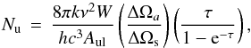 (1)where W is the velocity-integrated main-beam brightness temperature, Aul the Einstein spontaneous emission coefficient, and τ is the optical depth of the transition. For molecules in LTE, both a line’s excitation temperature and a molecule’s rotation temperature, which determines its relative energy level populations, equal the kinetic temperature (≡T); the population in each level is then given by the Boltzmann distribution:
 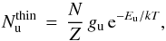 (2)where
  corresponds to optically-thin emission, ignoring the τ term in Eq. (1); N is the total column density, Eu is the upper energy level, gu is the statistical weight, and Z is the partition function. Thus, under the assumption of LTE, and with knowledge of T, we can obtain the total molecular column density from the column density of any single transition:
 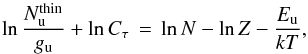 (3)where, following Goldsmith & Langer (1999), we have equated the optical-depth correction factor τ/ (1−e− τ) to Cτ, and Nu is calculated from the first two factors in Eq. (1). To evaluate the population diagrams numerically, the transition frequencies, upper energy levels, Einstein spontaneous emission, and statistical weights (ν, Eu, Aul, gu) for the 12CO and 13CO molecules were calculated using physical quantities from Schöier et al. (2005) and found to be highly consistent with the data from HITRAN (Rothman et al. 2009).
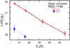 |
Fig. 8 Rotation or population level diagram for NGC 1140. A beam correction has been applied to the integrated intensities (see Sect. 4 for more details). Both 12CO and 13CO transitions are shown, as indicated by open (red) circles and filled (blue) squares, respectively. The gray dashed line for 12CO corresponds to the best-fit regressions; the temperature for 13CO is ill determined with only two transitions, so we fixed it to the 12CO value of Tex = 18.1 K. |
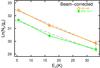 |
Fig. 9 Rotation or population level diagram for UM 448 and NGC 7077. A beam correction has been applied to the integrated intensities (see Sect. 4 for more details). The gray dashed line corresponds to the best-fit regression; as shown by the legend, the galaxies are differentiated by different symbols for 12CO emission (open (orange) circles and filled (green) circles, for UM 448 and NGC 7077, respectively). |
We first assume that the emission is optically thin, with τ ≪ 1 (Cτ = 1). A CO population diagram with this assumption for NGC 1140 is shown in Fig. 8, including the two available 13CO transitions. Here, as elsewhere, we have used the velocity-integrated Tmb corrected to a 22′′ beam size as described in Sect. 4 and Appendix A. By fitting the ln(Nu/gu) vs. Eu values with a linear regression (shown as a gray dashed line), we were able to infer the total 12CO and 13CO column densities and temperatures: T12CO = 18.1 ± 1.0 K; log (N12CO) = 14.7 cm-2; T13CO = 15 K. With only two transitions, the 13CO temperature is ill determined, so we fixed it to T12CO and obtained log (N13CO) = 13.6 cm-2.
We then attempted to correct for optical depth effects, according to Goldsmith & Langer (1999, their Eq. (27)): the largest correction term Cτ is for 12CO(4–3) with Cτ = 1.01, and the largest optical depth τ ~ 0.002. If we take these results at face value, and infer the 12CO/13CO abundances by taking the ratio of the total column densities, we obtain a value of 12CO/13CO ~ 12–13. To our knowledge this is one of the lowest values ever inferred for a galaxy, but cannot be considered reliable because of the assumption of optically thin gas in the LTE analysis. We will explore this further in Sects. 7.3 and 8.
The population diagrams under the optical-thin assumption for UM 448 and NGC 7077 (the only other galaxies for which we have 12CO(3–2) detections) are shown in Fig. 9. The observations were corrected for beam dilution as described in Sect. 4 and Appendix A. Again, from the best-fit regression, we infer T and total NCO column densities: T12CO = 10.8 ± 0.8 K and log (N12CO) = 15.0 cm-2 for UM 448; and T12CO = 12.3 ± 2.0 K and log (N12CO) = 14.7 cm-2 for NGC 7077. As for NGC 1140, we inferred the optical depths for the various transitions, and for both galaxies find that the largest τ is for the J = 2−1 transition with τCO = 0.001 (NGC 7077) and τCO = 0.002 (UM 448).
 |
Fig. 10 RADEX models (with ΔV = 20 km s-1) of 12CO line ratios plotted against Tkin: the left panel shows 12CO(2–1)/12CO(1–0) and the right 12CO(3–2)/12CO(1–0). The observations of NGC 1140, shown as a (black) filled circle, have been corrected for beam dilution assuming an exponential source distribution as described in Sect. 4 (see also Figs. 3 and 4). The approximate best-fit RADEX model for NGC 1140 (see Sect. 7.3) is shown in both panels as (purple) solid curves that coincide very well with the observations of NGC 1140. Also shown are three additional parameter combinations of 12CO column density N12CO and volume density nH2. The R31 parameter space occupied by the other galaxies (like Fig. 4, no beam corrections) is shown in the right-hand panel as a hatched region and solid horizontal lines (NGC 7077, UM 448, and an upper limit for Mrk 996). |
7.2. Modeling 12CO line ratios with RADEX
To better understand the observed 12CO line ratios in the galaxies in our sample, in particular the high ratio of NGC 1140 compared with other, more metal-rich, galaxies (see Figs. 3, 4), we have plotted the line ratios predicted by RADEX as a function of Tkin in Fig. 10 (R21 and R31 for NGC 1140 have been corrected for beam dilution as described in Sect. 4 and Appendix A). Two sets of column densities N12CO and volume densities nH2 are illustrated in the figure; the solid (purple, upper) line passing through the locus of NGC 1140 corresponds to the approximate best-fit RADEX model described in Sect. 7.3.
It is evident from Fig. 10 that the combination of moderately low column density (and thus low τCO) and high nH2 is a necessary ingredient for the high line ratios observed in NGC 1140. Line ratios would be high also in the case of high N12CO and high nH2 (see lower blue solid line), but only at high temperatures; this is the case in NGC 1068 where gas is warm and dense in the circumnuclear disk around the active nucleus (Viti et al. 2014). We discuss below in Sect. 7.3.3 why we consider high temperatures in NGC 1140 to be unlikely. In the case of more moderate nH2 (here illustrated as 104 cm-3), there is no Tkin that can sufficiently excite the upper J level.
The remaining galaxies for which we have 12CO(3–2) observations (Mrk 996, NGC 7077, UM 448) are also shown in the right panel of Fig. 10. The R31 values of these are less extreme, and can be well modeled with H2 volume densities as low as 104 cm-3. In these galaxies, the gas does not necessarily have to be cool and optically thin (i.e., low N12CO) in order to achieve the observed R31; it can be warmer and have a higher column density than in NGC 1140.
7.3. RADEX models for NGC 1140
To determine the excitation conditions of the molecular gas in NGC 1140, we have fitted the six 12CO and 13CO detected transitions with the radiative transfer code RADEX developed by van der Tak et al. (2007), using the uniform sphere approximation to calculate the escape probabilities. A one-zone model was adopted, namely the kinetic temperature and H2 volume density were required to be the same for all molecules, implying that all transitions sample the same gas. We calculated RADEX predictions for ΔV =10 and 20 km s-1, covering the following range of parameters sampled in logarithmic steps6:
-
H2 volume densitiesnH2 = 102−108 cm-3;
-
kinetic temperature Tkin = 5−200 K;
-
CO column densities NCO = 1012−1020 cm-2.
All parameters were calculated assuming a cosmic microwave background radiation temperature of T = 2.73 K. The 13CO abundance was included in the calculation through a second RADEX grid for the isotope; the column density N13CO was adjusted by sampling a range of abundances (from N12CO/N13CO = 1 to 100), and refining the fineness of the grid once the initial best-fit parameters were established. Ultimately, ≳400 000 total models in the combined 12CO +13CO grid were sampled.
The observed emission is generally only a small fraction of integrated line intensity from RADEX (and Large-Velocity Gradient, LVG) models. The fraction of these two quantities, F = (ΔνobsTobs)/(ΔVmodelTmodel), is the filling factor. We incorporated F as a free parameter in the models, and fit the grid of RADEX models via a χ2 minimization technique (e.g., Nikolić et al. 2007): 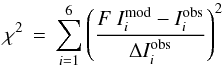 (4)where
  is the velocity-integrated Tmb of the ith transition,
  the ith model prediction, and
  are the 1σ uncertainties given in Table 4.
We also experimented with a minimization technique not including the filling factor F, but rather based on line ratios: 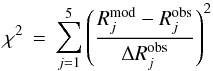 (5)where
  is the jth velocity-integrated temperature ratio,
  is the corresponding model line ratio, and
  are the 1σ uncertainties. These fits do not explicitly require equality of the filling factor F and thus may be more accommodating. We experimented with several sets of line ratios, in order to avoid potentially biasing the fits to any of the individual ratios.
As described in Sect. 4, we explored two different methods for correcting the velocity-integrated Tmb (and uncertainties) to a 22′′ beam size: (1) analyzing the cool-dust distribution and assuming that the molecular gas is distributed like the dust (see Appendix A); and (2) assuming the molecular gas is distributed in a Gaussian, and letting the Gaussian’s FWHM (θs) be a free parameter in the fit (see Appendix B). We used both methods to calculate the observed in Eqs. (4), (5). In the first case based on the fitted exponential function of the dust emission, were calculated independently of the fitting procedure. Thus for the six intensities (Eq. (4)), we fit five parameters (nH2, Tkin, NCO(12CO), [12CO]/[13CO], F), and for the five independent line ratios (Eq. (5)), we fit four parameters (same as before, but not including F). For the second case of Gaussian beam corrections, were calculated within the fit procedure; we explored θs ranging from 2′′ to 40′′, and narrowed the step size in successive iterations. Thus for the Gaussian beam corrections, the fitting procedure comprised an additional parameter, θs, and the minimum χ2 value includes this dependence. All the χ2 values quoted here are not reduced, but rather the total summed χ2.
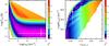 |
Fig. 11 RADEX fit χ2 surface (for the “Set 1” line ratios) with the exponential beam correction as a function of Tkin and nH2 in the left panel, and as a function of N12CO and τ(12CO(1–0)) in the right. The RADEX models shown here have ΔV = 20 km s-1. The associated χ2 values are shown as a side-bar color table. The χ2 color table in the right panel is different from the left because the interpolation used for the graphic display suffers from the coarser resolution in column density. The best-fit values are shown as an open (white) circle; the error bars shown consider a slightly more limited range in χ2 respect to Table 6. |
Table 6 gives the best-fit parameters obtained for NGC 1140. The different fitting methods and even the different beam correction approaches give very similar results, namely cool temperatures, high volume densities, low CO opacities, and low 12CO/13CO abundance ratios. The main difference among the fits is the CO column density, N12CO, which for a given ΔV varies by a factor of ~4. Because the opacity in the RADEX models τ ∝ Nco/ ΔV, and τ governs the line ratios and thus must remain relatively constant, for higher ΔV, N12CO is consequently higher within the resolution of our RADEX grid. For higher N12CO, the filling factor F is also commensurately lower, which we will discuss in Sect. 7.3.1. In any case, the low values of χ2 imply that a one-zone spherical cloud with uniform physical properties gives a good fit to the molecular gas emission in NGC 1140. The extremely low 12CO/13CO abundance ratio of ~8–20 is obtained for NGC 1140 even with a non-LTE analysis; we discuss this unexpected result further in Sect. 8.1.
Figure 11 shows the χ2 surface for the Set 1 line ratios7 with the exponential beam correction as a function of the fitted parameters (Tkin vs. nH2 in the left panel, and N12CO vs. τ[12CO(1–0)] in the right). In both panels, the error bars correspond to χ2 ≲ 1 at the best-fit value, rather than the full posterior range given in Table 6. It can also be seen from Fig. 11 that the parameters are fairly well constrained by the model; specifically, the volume density nH2 cannot be much lower than ~105 cm-3, and because of the well-known degeneracy between Tkin and nH2, the temperature also cannot be much greater than ~20 K.
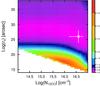 |
Fig. 12 RADEX fit χ2 surface (for the “Set 1” line ratios, assuming the Gaussian-derived beam correction factors) as a function of N12CO and Gaussian FWHM θs in the left panel, The RADEX models shown here have ΔV = 20 km s-1; the associated χ2 values are shown as a side-bar color table. The best-fit values are shown as an open (white) circle; the error bars shown consider a slightly more limited range in χ2 respect to Table 6. |
Best-fit RADEX parameters for NGC 1140.
Figure 12 gives the χ2 surface for the Set 1 line ratios using the Gaussian beam correction plotted against the 12CO column density N12CO and the Gaussian FWHM θs. The fit is somewhat sensitive to the assumed θs; for θs ≲ 15′′ and for θs ≳ 34′′, χ2> 10, and thus is not plotted. The best-fit Gaussian sizes range from 26′′ to 31′′, implying that under the assumption of a Gaussian distribution, the macroscopic size of the emission is ≳2 kpc. This would imply that the CO emission is more extended than the dust (FWHM(rs) ~ 850 pc, see Appendix A), which seems unlikely. In any case, even the largest CO beam is sampling less than half of the galaxy ISM; as shown in Fig. A.1, 50% of the dust emission lies within an effective radius (diameter) of ~20′′ (40′′, 3.8 kpc).
It should be emphasized that small χ2 values are not easy to achieve, even with several trials with many different formulations of beam corrections, in addition to the ones described in Sect. 4 and in Appendices A and B. The small χ2 values of the fits in Table 6 are telling us that for reasonable assumptions for beam corrections, the single-zone RADEX models can well accommodate the data. Moreover, the physical conditions inferred from the different fitting techniques are mutually consistent, independently of the kind of beam correction. Because of this similarity, in what follows, we will use the exponential beam corrections described in Appendix A; the virtue of these is that they can be measured or estimated for all the galaxies observed, under the assumption that on kpc scales the molecular gas is following the dust.
7.3.1. Filling factor
The mean 12CO line width of the various components in NGC 1140 (see Table 4) is ~21 km s-1; we thus prefer the RADEX fits with ΔV = 20 km s-1. For ΔV = 20 km s-1, fitting the intensities as in Eq. (4) gives a best-fit filling factor F of 0.10 ± 0.06. This best-fit F is rather large, but related to the somewhat low N12CO value of 1015.8 cm-2; as discussed below, the fits of the line ratios as in Eq. (5) give higher N12CO thus consequently lower, possibly more realistic, values of F.
For the line-ratio fits, the best-fit RADEX model for NGC 1140 predicts a velocity-integrated brightness temperature TB(12CO(1–0)) = 21.0 K km s-1; from Table 4, we have a beam-corrected velocity-integrated Tmb of 0.56 K km s-1. Dividing the two values gives a nominal filling factor of ~0.03. Similar filling factors are derived for the other transitions including 13CO, as a consequence of the assumption of a single-zone model. If we compare with the model from the “other” ΔV = 20 km s-1 line-ratio fits (see Table 7.3), with lower N12CO and τ (see Table 6), we obtain a slightly higher value, F ~ 0.04. Using the main-beam peak temperatures rather than velocity-integrated values (see Table 4), and adjusting to the common 22′′ beam size, gives filling factors of ~0.01.
These filling factors of a few percent for the molecular gas in NGC 1140 are similar to those found from high-resolution ALMA maps of 30 Doradus in the Large Magellanic Cloud (LMC, Indebetouw et al. 2013). They are also similar to those obtained by a similar χ2 analysis of non-LTE models of single-dish line ratios in the SMC and the LMC (Nikolić et al. 2007); these last are as high as ~0.14 (for what they consider to be good fits with χ2 ≲ 2), consistent with F = 0.1 for NGC 1140 obtained from the intensity fitting.
7.3.2. CO excitation ladder
The modeled CO excitation ladders for NGC 1140 are shown in Fig. 13. As in Fig. 10, the observations have been corrected for beam size as described in Sect. 4 and Appendix A. The line segments show the best-fit RADEX model for both 12CO and 13CO transitions adopting the best fit for the Set 1 line ratios with ΔV = 20 km s-1; the blue area corresponds to the range of ratios allowed by the models (for χ2 = χ2(min) + 1). The similar 12CO and 13CO slopes for NGC 1140 (the data points follow parallel lines) suggest that even the 12CO emission may be optically thin, as also implied by the best-fit results in Table 6. The CO gas is in an excited state, more similar to the center of M 82 (Weiß et al. 2005) than to the Milky Way (e.g., Carilli & Walter 2013). This is not a surprising result given the population of SSCs in the nuclear region of NGC 1140.
The low optical depths of even the 12CO lines steepen the excitation ladder at low J, steeper than ν2 as would be expected for thermalized, optically thick lines. The shape is an indirect consequence of the normalization to J = 1–0, due to the increase of τCO with increasing J up to the inflection in the excitation. Because 12CO(1–0) has the smallest τ of the 12CO transitions, with a different normalization, it would drop below the ν2 trend. The results of the RADEX fit (see Table 6) are telling us that the J = 4 level is sparsely populated because of the decreased τCO relative to the lower-J transitions; this produces the flattening in the excitation ladder.
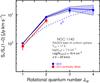 |
Fig. 13 RADEX best-fit model compared to observations for the CO excitation ladder of NGC 1140; the observations have been corrected for beam size as described in Sect. 4, and normalized to the CO(1–0) flux. The observations are shown as filled blue circles (12CO) and red squares (13CO), and the range of the allowed RADEX models by the light-blue region (for 12CO); 13CO points have arbitrarily offset relative to 12CO for clarity. The dashed curve shows the ν2 behavior (here normalized to J = 1) expected for optically-thick emission. |
7.3.3. Atomic carbon
We have performed additional RADEX fits to the 12CO and [Ci](1–0) emission, both with intensities as in Eq. (4) and with ratios (Eq. (5)). Fitted parameters include, as before, (nH2, Tkin, NCO(12CO), F), but now [12CO]/[12C], rather than [12CO]/[13CO]. Here, again, the implicit assumption is that atomic carbon and CO occupy the same volume, and are uniformly intermixed within an ISM of a single H2 kinetic temperature and volume density; such an assumption is consistent with the findings of Requena-Torres et al. (2016) for Hii regions in the SMC and of Okada et al. (2015) for the LMC. The results of the fits are given in Table 6 and shown graphically in Fig. 14 where the χ2 surfaces (in logarithmic terms) are shown as a function of nH2 and NCI(1−0) column density. As for the previous CO analysis, we prefer the ΔV = 20 km s-1 fits, roughly the mean component line width observed in NGC 1140.
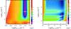 |
Fig. 14 RADEX fit of the χ2 (logarithmic) surface of the [Ci]/12CO fits as a function of nH2 and NCI(1−0); the left panel shows the intensity fits (Eq. (4)) and the right the ratio ones (Eq. (5)). The RADEX models shown here have ΔV = 20 km s-1. The associated Log(χ2) values are shown as a side-bar color table. The best-fit values are shown as an open (white) circle; the error bars shown consider a slightly more limited range in χ2 respect to Table 6. |
The intensity fit of the 12CO and [Ci] emission gives parameters very similar to the CO fit, although the inferred nH2 for the [Ci](1–0) fit is lower. On the other hand, the fit to the [Ci](1–0) ratios (with 12CO) gives higher Tkin, lower nH2, and 25 times higher NCO, higher than any other fit we performed. Folding in the best-fit [12CO]/[12C] abundance ratio, which varies by a factor of ~3 between the two fits, shows that the best-fit column density of atomic carbon NC is also different for both fits: ~1017.3 cm-2 in the intensity case and ~1018.2 cm-2 for the ratios. Consequently, the filling factors for the two fits also differ. The best-fit F for the [Ci] intensity fits is 0.10 as for (the intensity fitted) CO, but for the [Ci] ratio fits, it is much lower, F ≲ 0.01. This is because the higher NCO requires a lower filling factor to accommodate the RADEX predictions with the observations. We found a similar behavior in Sect. 7.3 for the CO ratio fits relative to the intensity ones. The reasons for the disagreement are unclear, although the low values of χ2 for all the [Ci] fits make it unlikely that the model is failing to capture the physical conditions in the clouds. In any case, these values of F are between 2 and 20 times lower than those found for [Ci] emission in the Magellanic Clouds by Pineda et al. (2017); however their observations probe physical scales more than 50 times smaller, so a comparison is not straightforward.
Independently of the disagreement, our RADEX fits for [Ci] all find that the atomic carbon column density must be larger than NCO, implying a [12CO]/[12C] abundance of <1. For the intensity fit, with lower NCO, this requires a very low [12CO]/[12C] of ~0.03, while for the ratio fit with higher NCO, [12CO]/[12C] ~ 0.1. This would indicate that atomic carbon is at least 10 times more abundant than 12CO in NGC 1140. Such a result would be consistent with the theoretical predictions of Bialy & Sternberg (2015) for interstellar ion-molecule gas-phase chemistry in galaxies; their models predict that [12CO]/[12C] abundance ratios decrease with decreasing metallicity and with higher ionization parameters. On the other hand, observational studies of luminous (metal-rich) galaxies found that atomic carbon is less abundant than CO, [12CO]/[12C] ~ 4–8 (e.g., Israel 2009; Israel et al. 2015). However, the observed [Ci](1–0)/12CO(4–3) ratio (in flux units) for NGC 1140 (~0.7) is more than 4σ higher than the mean of the galaxies observed by Israel et al. (2015), so the relatively high abundance of atomic carbon is perhaps not altogether surprising. Although our [Ci](1–0) detection is marginal (~3σ, see Table 4), to reduce the inferred [12CO]/[12C] ratio to unity or less would require a reduction in the [Ci](1–0) intensity by more than a factor of 10; this seems unlikely given the trends shown in Fig. 5.
Independent one-zone model fitting of the 12CO, 13CO, and [Ci](1–0) emission of NGC 1140 gives similar physical conditions. Specifically, by fitting a vast grid of LVG models (Weiß et al. 2007) to the NGC 1140 data, and considering dust continuum, and molecular and atomic abundances relative to H2, we obtain high densities (nH2 ≳ 105 cm-3), cool temperatures (Tkin ~ 20 K), low [12CO]/[13CO] abundance ratios (~13), low [12CO]/[12C] abundance ratios (~0.13), and moderate column densities (NCO ~ 5 × 1016 cm-2), similar to the RADEX results. However, with these models, a “warm” solution with Tkin ~52 K is also possible. This solution would result in higher abundance ratios ([12CO]/[13CO] ~ 36, [12CO]/[12C] ~ 0.3), and higher NCO (~7 × 1017 cm-2). Nevertheless, in this case there would be an unrealistically low gas-to-dust mass ratio (GDR), ~62; this is lower than even the Milky Way (GDR ~ 100, Draine et al. 2007), which is unlikely considering the low metallicity of NGC 1140. With Z/Z⊙ ~ 0.3 for NGC 1140, and given the linear trend of GDR with metallicity in this abundance range (e.g., Rémy-Ruyer et al. 2014), we would expect a GDR of ~300, not far from the GDR of ~380, inferred from the “cool” solution obtained with the Weiß et al. (2007) LVG models. Thus, the “cool” solution with Tkin ~ 20 K seems more likely for NGC 1140.
The “warm” solution with the Weiß et al. (2007) LVG models for 12CO, 13CO, and [Ci](1–0) is not far from the “warm” solution (with Tkin ~ 38 K) that emerged from the RADEX fitting of [Ci](1–0) and 12CO line ratios (see Table 6). However, our RADEX models for 13CO and 12CO do not allow the higher Tkin found with the Weiß et al. (2007) models; we obtain χ2> 10 for Tkin > 46 K, and a mean χ2 of ~6–7 for 40 ≤ Tkin ≤ 46 K, compared to χ2 values of <1 for our best fits. Based on the much lower χ2 values for the CO fits with cool Tkin, we do not consider further the “warm” RADEX fits. Observations of higher-J CO lines and [Ci](2–1) would help settle this potential ambiguity.
Combined with the [12CO]/[13CO] abundance ratio of ~10–12 found above (see also Sect. 7.1), this would imply a [12C]/[13CO] abundance ratio of ≳100–300, within the range of values found by Israel et al. (2015) for galaxies with low CO/[Ci](1–0)] ratios. However, this may be a specious comparison because of the unusually low [12CO]/[13CO] abundance ratio which, in some sense, compensates for the extremely low [12CO]/[12C] found here for NGC 1140. As already mentioned, we discuss further the low [12CO]/[13CO] abundance ratio found for NGC 1140 in Sect. 8.1.
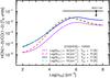 |
Fig. 15 RADEX models of HCN(1–0)/12CO(1–0) line ratios plotted against nH2, and assuming [CO]/[HCN] = 105. Here the ΔV = 20 km s-1 models are illustrated. The upper limit HCN(1–0)/12CO(1–0) ratio for NGC 1140, shown as a (black) filled circle, has not been corrected for beam dilution because of the similar beam sizes for the two transitions. The approximate best-fit RADEX model for NGC 1140 is shown as a (purple) solid curve that is consistent with the non-detection of HCN(1–0). Also shown are three additional parameter combinations of 12CO column density N12CO and volume density nH2. |
7.3.4. Modeling HCN with RADEX
We did not detect HCN(1–0) in NGC 1140, even though the RADEX best fit suggests that there is dense gas in this galaxy. Figure 15 shows the predictions of RADEX models for the HCN(1–0)/12CO(1–0) line ratio plotted against H2 volume density, nH2 and assuming [CO]/[HCN] = 105. The implicit assumption here, almost certainly incorrect, is that the filling factor of the emitting gas is the same in both transitions. Figure 15 suggests that the abundance ratio [CO]/[HCN] must be high ≳105. Relative to the best-fit RADEX model for NGC 1140, [CO]/[HCN] = 105 corresponds to an HCN column density of ~2 × 1011 cm-2, an order of magnitude lower than in diffuse clouds in the Galaxy (Liszt & Lucas 2001).
The upper limit (UL) for the HCN(1–0)/12CO(1–0) line temperature ratio of NGC 1140 is ~0.1, higher than the detected HCN(1–0)/12CO(1–0) ratio of ~0.05 in the prominent star-formation region N 113 of the LMC (Wang et al. 2009). Thus, even after 18 h with the IRAM 30 m, our observations are not able to constrain the HCN content of NGC 1140. More observations of dense-gas tracers are needed at low metallicity, especially outside the Local Group where conditions can be even more extreme than in the massive star-forming regions in the Magellanic Clouds.
8. Discussion
Unlike some previous work covering a similar range of CO J values (e.g., Meier et al. 2001; Israel 2005; Nikolić et al. 2007), our one-zone non-LTE models give very good fits to the CO and atomic carbon emission in NGC 1140. Part of this success is almost certainly due to the lack of high-J transitions in our data set; we are fitting only the cool, dense clouds in this galaxy, while there may be a substantial contribution of warmer, more diffuse gas. It may also be a consequence of the extreme conditions in this galaxy. None of the six dwarf galaxies observed by Cormier et al. (2014) in 12CO(1–0) and 12CO(2–1) have R21 > 1, independently of the beam size of the observations or the upper limits. The N 113 region in the LMC has R21 ≲ 1 after beam deconvolution (R21 ~ 1.2 before, see Wang et al. 2009), and Minamidani et al. (2008) found maximum values of R31 ≳ 1 in only a handful of the 33 LMC regions observed. These ratios are much higher in NGC 1140 (R21 = 2.1, R31 = 1.7, see Figs. 3, 4, and Table A.1), independently of the beam corrections applied. Because of these high line ratios, and the implied more extreme physical conditions dominating the ISM of this galaxy, one-zone models may be more effective.
The CO excitation in NGC 1140 is starburst-like, similar to M 82, but as mentioned before, this is not particularly surprising given the presence of at least 6 SSCs within its central region (de Grijs et al. 2004; Moll et al. 2007). However, unlike M 82, where the gas is warm (Tkin ~ 60−200 K) and not particularly dense (nH2 ~ 103 cm-3, Weiß et al. 2005; Mühle et al. 2007), in NGC 1140 the gas is dense and cool. Given the relatively high excitation, it is not straightforward to understand why the CO has not been photo-dissociated through the intense radiation field, although as discussed below, the dense, small-filling factor clouds may be one part of the explanation. High atomic gas columns may also contribute to self-shielding as discussed below and suggested by Wong et al. (2009) for the LMC.
Finding evidence for cool, dense gas, nH2 ≳ 106 cm-3 in NGC 1140 was unexpected. However, at least one other low-metallicity galaxy outside the Local Group shows similar properties. In Haro 11, PDR modeling (Cormier et al. 2012, 2014) also suggests that the molecular gas is dense, with hydrogen densities nH ~ 105−6 cm-3. The Cormier et al. (2014) PDR model for Haro 11 implies that CO emission is produced at intermediate depths within the cloud (3 <AV< 6 mag), and for larger AV, the gas temperature is ~30 K, somewhat warmer than the (non-LTE) gas temperature Tkin of ~17 K we find for NGC 1140.
Another unexpected result is the low optical depth of the 12CO transitions. Our RADEX fits (see Table 6, ΔV = 20 km s-1) suggest that the 12CO and 13CO transitions have a maximum τCO ~ 0.2 for 12CO(3–2). The best fit of 12CO with [Ci] gives higher optical depths, with τCO ~ 1 for 12CO(3–2) but lower for the other transitions. Apparently even these low optical depths allow sufficient self-shielding for detectable 12CO and 13CO emission. This could be possible because the clouds are dense and occupy only a small fraction of the macroscopic source size (see Sect. 7.3.1).
It could also be that high column densities are contributing to the shielding of the molecular gas. Hunter et al. (1994a) find a peak Hi column NHI of 2.4 × 1021 cm-2 (averaged over a 30″ × 37″ beam), ~10 times higher than the NH2 of 2 × 1020 cm-2 estimated from NCO ~ 1016 cm-2, assuming a roughly solar abundance ratio [H2]/[CO] ~ 5 × 10⁻⁵ (e.g., Sakamoto 1999). Even the disk-averaged NHI in NGC 1140 of ~1021 cm-2 (Fumagalli et al. 2010) is 5 times higher than the H2 column that we would infer from NCO. As proposed by Wong et al. (2009), high Hi columns may even be necessary (but not sufficient) for the detection of CO in low-metallicity galaxies. However, the LVG abundance fits using the models of Weiß et al. (2007) indicate that the [CO]/[H2] abundance ratio in NGC 1140 is extremely low: ~100 times lower than solar for the “cool” solution ([CO]/[H2] ~ 8 × 10⁻⁷). This would imply that the H2 columns could be comparable to, if not exceed, the Hi, thus dominating the column density contribution necessary for self-shielding.
Such a low [CO]/[H2] abundance and cold Tkin in NGC 1140 could be the result of a high level of photo-dissociation of CO, leaving only the densest, best shielded cores. This is a similar situation to ammonia (NH3) in the LMC where it is only detected in N 159 W (Ott et al. 2010). In this region, the NH3 is cold with Tkin ~ 16 K, and has very low abundance; NH3 abundance is between 1.5 and 5 orders of magnitude lower than observed in Galactic star-forming regions, but similar to that found in the late-stage starburst M 82 (Weiß et al. 2001). NH3 is particularly sensitive to UV radiation (Sato & Lee 1983), but formaldehyde (H2CO) is less vulnerable to photo-dissociation than NH3, and in N 159 W is warmer, Tkin ~ 30–35 K (Tang et al. 2017). The implication is that H2CO is sampling regions that are more exposed to radiation of young massive stars, while NH3 resides in the most shielded knots of dense gas (Tang et al. 2017). The stronger radiation field in NGC 1140 from the concentration of SSCs would annihilate NH3, and possibly also H2CO, but CO could survive, thus playing the role that NH3 plays in the LMC, tracing the surviving cool pockets of dense gas.
Such a scenario may occur in any specific low-metallicity star-forming region. That it is seen over a ~2 kpc area of a galaxy with six SSCs requires that the evaporation of dense molecular gas occurs roughly simultaneously. Thus, galaxies like NGC 1140 are probably rare. Consistently with observations, the starburst must also be either quite young (all activity is occurring at almost the same time) or the last one of several possibly very short starburst episodes (e.g., de Grijs et al. 2004; Moll et al. 2007). With 6 SSCs, all of them clearly surpassing 30 Doradus in the LMC, this last starburst episode must then be at least (if not the only one) the strongest one. More extensive observations of molecular tracers are necessary to test this scenario, and constrain models of CO/H2 abundance ratios in NGC 1140, and, more generally, in metal-poor starbursts.
Our RADEX fits with 12CO and [Ci] also give an unusually high atomic carbon abundance (see Sect. 7.3.3), C/CO ≳ 10. This result is premised on the assumption that [Ci] and CO occupy the same volume in a cloud characterized by a single kinetic temperature and volume density (e.g., Okada et al. 2015; Requena-Torres et al. 2016). Such a high [Ci] abundance relative to CO is more extreme than found in the SMC with the LVG analysis of Requena-Torres et al. (2016); there the clouds tend to be less dense (nH2 ~ 104 cm-3), and warmer (Tkin ~ 30−50 K), although of similar CO column density (NCO ~ 2−4 × 1016 cm-2, see also Nikolić et al. 2007). Spatially-resolved observations of [Ci] and CO in NGC 1140 would help understand whether the high [Ci] abundance we find is dictated by a different spatial distribution relative to CO, unlike what is observed in the Magellanic Clouds.
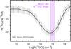 |
Fig. 16 12CO/13CO abundance ratio plotted against N(12CO). The shaded rectangle shows the ranges of values from RADEX fits (ΔV = 20 km s-1) of NGC 1140. The solid line corresponds to the models of the 12CO/13CO abundance ratio vs. the 12CO column density by Szűcs et al. (2014). The error bars for these models (vertical black lines) are (very roughly) estimated from their Fig. 8. |
8.1. 13CO charge-exchange reactions and fractionation
Another surprising result from our RADEX analysis of NGC 1140 is the unusually low [12CO]/[13CO] abundance ratio, ~8–20, lower even than the value of ~24 found in the Galactic Center (Langer & Penzias 1990). Isotopic ratios are generally governed by two competing processes: photo-selective dissociation that would tend to decrease the relative 13CO abundance, and low-temperature carbon isotope exchange reactions that would tend to increase it.
Low [12CO]/[13CO] abundance ratios are typically found in older intermediate-mass stellar populations (≳500 Myr), in which 13C is produced in nuclear reactions in the cores of asymptotic giant branch (AGB) stars, and “dredged up” through convective mixing where it is ejected into the ISM in stellar winds (e.g., Milam et al. 2005, 2009). However, the SSCs in NGC 1140 are quite young, with ages ranging from ~5 to 12 Myr, and the overall starburst is younger than ~55 Myr (de Grijs et al. 2004; Moll et al. 2007). These young ages make it unlikely that the isotopic ratio in NGC 1140 has been lowered by stellar reprocessing (e.g., Boothroyd & Sackmann 1999; Pavlenko et al. 2003; Henkel et al. 2014).
Instead, the extremely low 12CO/13CO abundance ratio for NGC 1140 could be explained by charge-exchange reactions, i.e., fractionation (e.g., Watson et al. 1976). Isotopic selective photo-dissociation of CO is effective only in diffuse gas (nH2 ≲ 100 cm-3); in denser regions with higher column density but moderate extinction (1 mag ≲ AV ≲ 3 mag), fractionation reactions become important:
 At intermediate NCO (and T ≲ 35 K), the rightmost (exothermic) reaction dominates, enhancing 13CO and leading to a reduced [12CO]/[13CO] abundance ratio. Thus, if molecular gas in low-metallicity galaxies is dense and cool, but with moderate NCO as in NGC 1140, it is possible that fractionation drives low 12CO/13CO ratios.
The low value of [12CO]/[13CO] we obtain for NGC 1140 is roughly consistent with (although slightly higher than) the trends of CO column density and 13CO fractionation found by Röllig & Ossenkopf (2013) and Szűcs et al. (2014). Figure 16 shows the trend of 12CO/13CO abundance ratio and 12CO column density given by Szűcs et al. (2014); the range of N(12CO) for NGC 1140 as estimated by the best-fit RADEX (and LTE) models is shown as a shaded rectangle. Szűcs et al. (2014) show that there is a “sweet spot” in NCO for maximizing the fractionation process, as long as the temperature barrier of ~35 K is not exceeded. Interestingly, the best-fit Tkin for NGC 1140 is ~16–18 K (see Fig. 11 and Table 6), consistent with the low temperatures necessary for optimizing 13CO fractionation. In NGC 1140, the low X(12CO)/X(13CO) abundance ratio could be fostered by the moderately low NCO and the low temperature, which in turn are probably related to the high nH2 volume density. We are pursuing an observational program to establish whether such a phenomenon is common in metal-poor starbursts.
8.2. The H2 mass for NGC 1140 revealed with atomic carbon
In Paper I, we derived the metallicity dependence for the CO-to-H2 conversion factor, αCO ∝ (Z/Z⊙)-2, which, at the metallicity of NGC 1140, is roughly equivalent to the exponential variation with abundance found by Wolfire et al. (2010). Here we compare the molecular mass for NGC 1140 using αCO with the molecular mass estimated from [Ci] luminosity according to Glover & Clark (2016). After correcting to a 22′′ beam size as in Table 4 (see also Table A.1), L′(CO) = 2.9 × 10⁶ K km s-1 pc2. Using αCO = 3.2 M⊙ (K km s-1 pc (not including helium, Saintonge et al. 2011), and scaling with (Z/Z⊙)-2 (see Paper I) for NGC 1140 (Z/Z⊙ = 0.31; 12 + log(O/H) = 8.18, and assuming 12 + log(O/H)⊙ = 8.69 from Asplund et al. 2009), we find a total molecular gas mass of ~9.3 × 10⁷ M⊙.
Glover & Clark (2016) use their hydrodynamical simulations of [Ci](1–0) emission to estimate H2 masses, and provide a [Ci] luminosity-to-H2 conversion factor. At the highest G0 modeled by Glover & Clark (2016), they obtain a mean value XCI = 8.8 × 1020 cm-2 (K km s-1)-1 for Z ~ Z⊙ and an approximately linear increase with decreasing metallicity. For NGC 1140 the [Ci](1–0) luminosity L′([Ci](1–0)) = 1.6 × 10⁶ K km s-1 pc2 (from Table 4, including the aperture correction for a 22′′ beam). Converting the Glover & Clark (2016)XCI to equivalent αCO units, we would find αCI = 53.2 M⊙ (K km s-1 pc2)-1 for 0.31 Z/Z⊙, and a resulting molecular mass MH2 of ~8.7 × 10⁷ M⊙. This value is within 10% of what we infer with the quadratic metallicity scaling of αCO, despite the larger observed [Ci](1–0)/12CO(1–0) ratio (see Sect. 5.3) relative to their models8. These values of molecular gas mass for NGC 1140 are within 15% of those estimated using the models of Weiß et al. (2007).
9. Summary and conclusions
We have presented 12CO observations of ten galaxies, with detections for eight. With metallicities ranging from 12 + log(O/H) ~ 7.7 to 8.4 (0.1 Z⊙ to 0.5 Z⊙), at and below the abundance of the SMC, this is the largest sample of metal-poor galaxies with CO detections so far obtained outside the Local Group. For one of the galaxies, NGC 1140, we report additional 13CO, [Ci](1–0), and HCN(1–0) measurements. Our main conclusions are the following:
-
After correcting for differences in beam sizes,NGC 1140 shows high velocity-integrated temperature ratios of 12CO(2–1)/12CO(1–0) (R21 = 2.1 ± 0.06) and 12CO(3–2)/12CO(1–0) (R31 = 2.0 ± 0.45, or R31 = 1.7 ± 0.39 with the correction to 22′′ beams), while the other galaxies have less extreme ratios (see Figs. 3, 4).
-
A comparison of dense-gas tracers such as 12CO(3–2) (of the four observed metal-poor galaxies) and HCN(1–0) (upper limit for NGC 1140) with data in the literature shows a deficit in 12CO(3–2) relative to SFR (see Fig. 7), similar to the 12CO(1–0) deficit found in Paper I. However, gas excitation at low metallicity measured by comparing 12CO(3–2) to 12CO(1–0) luminosities seems similar to that of more metal-rich systems. HCN(1–0) was observed but not detected in NGC 1140. The lower limit of HCN(1–0) for NGC 1140 may be due to a combination of stellar feedback (e.g., Hopkins et al. 2013) and an extremely high [CO]/[HCN] abundance ratio (≳105) probably because of the low metallicity (see Fig. 15).
-
Fitting LTE models to the 12CO(3–2), 12CO(2–1), and 12CO(1–0) emission in NGC 1140, NGC 7077, and UM 448 suggests that CO column densities are moderate and temperatures are low. These fits also suggest low optical depths, but the lack of higher-J lines for NGC 7077 and UM 448 prevents confirming this as a general result with radiative-transfer models.
-
Fitting physical models (RADEX) of the 12CO and 13CO emission in NGC 1140 suggests that the molecular gas is cool (Tkin ≲ 20 K), dense (nH2 ≳ 106 cm-3), with moderate CO column density (NCO ~ 1016 cm-2) and low filling factor (F ~ 0.01−0.1). 12CO optical depths are fairly low (τCO ≲ 0.2), and we speculate that the CO survives photo-dissociation because of the high Hi column density in this galaxy. The molecular excitation in NGC 1140 is starburst-like, similar to M 82 (see Fig. 13).
-
The [12CO]/[13CO] abundance ratio in NGC 1140 inferred from the fit is very low, ~8–20, lower even than the value of ~24 found in the Galactic center (Langer & Penzias 1990). Because the starburst in NGC 1140 is quite young, it is difficult to interpret this low ratio as due to stellar reprocessing by older intermediate-mass populations (e.g., Milam et al. 2005, 2009). Instead, we attribute it to enhanced CO fractionation, from the combination of moderate column densities and cool gas (see Fig. 16), as predicted by the chemical models of Röllig & Ossenkopf (2013) and Szűcs et al. (2014).
-
Fitting RADEX models of the 12CO and [Ci](1–0) emission in NGC 1140 gives physical conditions similar to the 12CO+13CO fits, although there is a possibility for warmer (Tkin ~ 38 K), less dense (nH2 ~ 104 cm-2) gas at higher column densities. Independent fitting results for NGC 1140 using the models of Weiß et al. (2007) give similar results. Both our RADEX fits and the LVG fits suggest that atomic carbon is at least 10 times more abundant than 12CO in NGC 1140.
For the first time outside the Local Group, the six CO transitions measured for NGC 1140, together with [Ci](1–0), have enabled an analysis of physical conditions in the molecular gas of a low-metallicity galaxy with at least 6 SSCs. The unusual [12CO]/[13CO] and [12CO]/[12C] abundance ratios, and the cool, dense gas at moderate column densities, may be the consequence of the SSCs in this galaxy and their feedback effect on the ISM. Future work will attempt to put this speculation on a more quantitative footing, both with models of ISM chemistry and with more observations of the molecular ISM in low-metallicity starbursts.
We assume the Asplund et al. (2009) solar abundance calibration of 12 + log(O/H) = 8.69.
This publication is based on data acquired with the Atacama Pathfinder Experiment (APEX). APEX is a collaboration between the Max-Planck-Institut für Radioastronomie, the European Southern Observatory, and the Onsala Space Observatory.
We do not apply beam corrections to the upper limit, because of the similarity of the HCN(1–0) and 12CO(1–0) beam sizes.
Here and throughout the paper we use the “robust” regression algorithm, effective for minimizing the effects of outliers, as implemented in R, a free software environment for statistical computing and graphics, https://www.r-project.org/
Temperature was sampled linearly.
“Set 1” was taken with the ratios relative to the adjacent lower-J line, specifically: [12CO(2–1)/12CO(1–0), 12CO(3–2)/12CO(2–1), 12CO(4–3)/12CO(3–2), 13CO(1–0)/12CO(1–0), 13CO(2–1)/13CO(1–0)]. See Table 6 for more details.
Acknowledgments
We acknowledge the anonymous referee for her/his useful comments and suggestions. L.K.H. is grateful to Carlo Giovanardi for interesting discussions and mathematical insights for the beam corrections. S.G.B. acknowledges economic support from grants ESP2015-68964-P and AYA2016-76682-C3-2-P. We warmly thank the IRAM staff, both in Granada and at Pico Veleta, for their capable management of the logistics and the telescope/receiver operations. We are also indebted to the APEX service observing team for their dedication in the challenging high-frequency observations obtained for NGC 1140. We gratefully acknowledge the International Space Science Institute (Bern) for hospitality during the conception of this paper. Heavy use was made of the NASA/IPAC Extragalactic Database (NED).
References
- Albrecht, M., Chini, R., Krügel, E., Müller, S. A. H., & Lemke, R. 2004, A&A, 414, 141 [NASA ADS] [CrossRef] [EDP Sciences] [Google Scholar]
- Asplund, M., Grevesse, N., Sauval, A. J., & Scott, P. 2009, ARA&A, 47, 481 [NASA ADS] [CrossRef] [Google Scholar]
- Barone, L. T., Heithausen, A., Hüttemeister, S., Fritz, T., & Klein, U. 2000, MNRAS, 317, 649 [NASA ADS] [CrossRef] [Google Scholar]
- Bayet, E., Gerin, M., Phillips, T. G., & Contursi, A. 2006, A&A, 460, 467 [NASA ADS] [CrossRef] [EDP Sciences] [Google Scholar]
- Bialy, S., & Sternberg, A. 2015, MNRAS, 450, 4424 [NASA ADS] [CrossRef] [Google Scholar]
- Bisbas, T. G., Papadopoulos, P. P., & Viti, S. 2015, ApJ, 803, 37 [NASA ADS] [CrossRef] [Google Scholar]
- Bisbas, T. G., van Dishoeck, E. F., Papadopoulos, P. P., et al. 2017, ApJ, 839, 90 [NASA ADS] [CrossRef] [Google Scholar]
- Bolatto, A. D., Jackson, J. M., & Ingalls, J. G. 1999, ApJ, 513, 275 [NASA ADS] [CrossRef] [Google Scholar]
- Bolatto, A. D., Jackson, J. M., Kraemer, K. E., & Zhang, X. 2000a, ApJ, 541, L17 [NASA ADS] [CrossRef] [Google Scholar]
- Bolatto, A. D., Jackson, J. M., Israel, F. P., Zhang, X., & Kim, S. 2000b, ApJ, 545, 234 [NASA ADS] [CrossRef] [Google Scholar]
- Bolatto, A. D., Jackson, J. M., Wilson, C. D., & Moriarty-Schieven, G. 2000c, ApJ, 532, 909 [NASA ADS] [CrossRef] [Google Scholar]
- Bolatto, A. D., Leroy, A. K., Rosolowsky, E., Walter, F., & Blitz, L. 2008, ApJ, 686, 948 [NASA ADS] [CrossRef] [Google Scholar]
- Bolatto, A. D., Wolfire, M., & Leroy, A. K. 2013, ARA&A, 51, 207 [Google Scholar]
- Boothroyd, A. I., & Sackmann, I.-J. 1999, ApJ, 510, 232 [NASA ADS] [CrossRef] [Google Scholar]
- Braine, J., & Combes, F. 1992, A&A, 264, 433 [NASA ADS] [Google Scholar]
- Buchbender, C., Kramer, C., Gonzalez-Garcia, M., et al. 2013, A&A, 549, A17 [NASA ADS] [CrossRef] [EDP Sciences] [Google Scholar]
- Buyle, P., Michielsen, D., de Rijcke, S., Ott, J., & Dejonghe, H. 2006, MNRAS, 373, 793 [NASA ADS] [CrossRef] [Google Scholar]
- Carilli, C. L., & Walter, F. 2013, ARA&A, 51, 105 [NASA ADS] [CrossRef] [EDP Sciences] [Google Scholar]
- Cohen, R. S., Dame, T. M., Garay, G., et al. 1988, ApJ, 331, L95 [NASA ADS] [CrossRef] [Google Scholar]
- Cormier, D., Lebouteiller, V., Madden, S. C., et al. 2012, A&A, 548, A20 [NASA ADS] [CrossRef] [EDP Sciences] [Google Scholar]
- Cormier, D., Madden, S. C., Lebouteiller, V., et al. 2014, A&A, 564, A121 [NASA ADS] [CrossRef] [EDP Sciences] [Google Scholar]
- de Grijs, R., Smith, L. J., Bunker, A., et al. 2004, MNRAS, 352, 263 [NASA ADS] [CrossRef] [Google Scholar]
- Draine, B. T. 1978, ApJS, 36, 595 [NASA ADS] [CrossRef] [Google Scholar]
- Draine, B. T., Dale, D. A., Bendo, G., et al. 2007, ApJ, 663, 866 [NASA ADS] [CrossRef] [Google Scholar]
- Elmegreen, B. G., Rubio, M., Hunter, D. A., et al. 2013, Nature, 495, 487 [NASA ADS] [CrossRef] [Google Scholar]
- Fukui, Y., Mizuno, N., Yamaguchi, R., et al. 1999, PASJ, 51, 745 [NASA ADS] [CrossRef] [Google Scholar]
- Fumagalli, M., Krumholz, M. R., & Hunt, L. K. 2010, ApJ, 722, 919 [NASA ADS] [CrossRef] [Google Scholar]
- Gao, Y., & Solomon, P. M. 2004, ApJ, 606, 271 [NASA ADS] [CrossRef] [Google Scholar]
- García-Burillo, S., Usero, A., Alonso-Herrero, A., et al. 2012, A&A, 539, A8 [NASA ADS] [CrossRef] [EDP Sciences] [Google Scholar]
- Gerin, M., & Phillips, T. G. 2000, ApJ, 537, 644 [NASA ADS] [CrossRef] [Google Scholar]
- Glover, S. C. O., & Clark, P. C. 2016, MNRAS, 456, 3596 [NASA ADS] [CrossRef] [Google Scholar]
- Goldsmith, P. F., & Langer, W. D. 1999, ApJ, 517, 209 [NASA ADS] [CrossRef] [Google Scholar]
- Gondhalekar, P. M., Johansson, L. E. B., Brosch, N., Glass, I. S., & Brinks, E. 1998, A&A, 335, 152 [NASA ADS] [Google Scholar]
- Graciá-Carpio, J., García-Burillo, S., Planesas, P., Fuente, A., & Usero, A. 2008, A&A, 479, 703 [NASA ADS] [CrossRef] [EDP Sciences] [Google Scholar]
- Greve, T. R., Leonidaki, I., Xilouris, E. M., et al. 2014, ApJ, 794, 142 [NASA ADS] [CrossRef] [Google Scholar]
- Henkel, C., Asiri, H., Ao, Y., et al. 2014, A&A, 565, A3 [NASA ADS] [CrossRef] [EDP Sciences] [Google Scholar]
- Hollenbach, D. J., Takahashi, T., & Tielens, A. G. G. M. 1991, ApJ, 377, 192 [NASA ADS] [CrossRef] [Google Scholar]
- Hopkins, P. F., Narayanan, D., Murray, N., & Quataert, E. 2013, MNRAS, 433, 69 [NASA ADS] [CrossRef] [Google Scholar]
- Hunt, L. K., Thuan, T. X., Izotov, Y. I., & Sauvage, M. 2010, ApJ, 712, 164 [NASA ADS] [CrossRef] [Google Scholar]
- Hunt, L. K., García-Burillo, S., Casasola, V., et al. 2015, A&A, 583, A114 (Paper I) [NASA ADS] [CrossRef] [EDP Sciences] [Google Scholar]
- Hunter, D. A., van Woerden, H., & Gallagher, J. S., III 1994, ApJS, 91, 79 [NASA ADS] [CrossRef] [Google Scholar]
- Indebetouw, R., Brogan, C., Chen, C.-H. R., et al. 2013, ApJ, 774, 73 [NASA ADS] [CrossRef] [Google Scholar]
- Israel, F. P. 2005, A&A, 438, 855 [NASA ADS] [CrossRef] [EDP Sciences] [Google Scholar]
- Israel, F. P. 2009, A&A, 493, 525 [NASA ADS] [CrossRef] [EDP Sciences] [Google Scholar]
- Israel, F. P., & Baas, F. 2002, A&A, 383, 82 [NASA ADS] [CrossRef] [EDP Sciences] [Google Scholar]
- Israel, F. P., & Baas, F. 2003, A&A, 404, 495 [NASA ADS] [CrossRef] [EDP Sciences] [Google Scholar]
- Israel, F. P., Baas, F., Rudy, R. J., Skillman, E. D., & Woodward, C. E. 2003, A&A, 397, 87 [NASA ADS] [CrossRef] [EDP Sciences] [Google Scholar]
- Israel, F. P., Rosenberg, M. J. F., & van der Werf, P. 2015, A&A, 578, A95 [NASA ADS] [CrossRef] [EDP Sciences] [Google Scholar]
- Johnson, K. E., Leitherer, C., Vacca, W. D., & Conti, P. S. 2000, AJ, 120, 1273 [NASA ADS] [CrossRef] [Google Scholar]
- Kepley, A. A., Leroy, A. K., Johnson, K. E., Sandstrom, K., & Chen, C.-H. R. 2016, ApJ, 828, 50 [NASA ADS] [CrossRef] [Google Scholar]
- Kobulnicky, H. A., Kennicutt, R. C., Jr., & Pizagno, J. L. 1999, ApJ, 514, 544 [NASA ADS] [CrossRef] [Google Scholar]
- Kramer, C., Jakob, H., Mookerjea, B., et al. 2004, A&A, 424, 887 [NASA ADS] [CrossRef] [EDP Sciences] [Google Scholar]
- Krips, M., Martín, S., Sakamoto, K., et al. 2016, A&A, 592, L3 [NASA ADS] [CrossRef] [EDP Sciences] [Google Scholar]
- Kuno, N., Sato, N., Nakanishi, H., et al. 2007, PASJ, 59, 117 [NASA ADS] [Google Scholar]
- Lada, C. J., Forbrich, J., Lombardi, M., & Alves, J. F. 2012, ApJ, 745, 190 [NASA ADS] [CrossRef] [Google Scholar]
- Langer, W. D., & Penzias, A. A. 1990, ApJ, 357, 477 [NASA ADS] [CrossRef] [Google Scholar]
- Lequeux, J., Le Bourlot, J., Pineau des Forets, G., et al. 1994, A&A, 292, 371 [NASA ADS] [Google Scholar]
- Leroy, A., Bolatto, A. D., Simon, J. D., & Blitz, L. 2005, ApJ, 625, 763 [NASA ADS] [CrossRef] [Google Scholar]
- Leroy, A., Cannon, J., Walter, F., Bolatto, A., & Weiß, A. 2007, ApJ, 663, 990 [NASA ADS] [CrossRef] [MathSciNet] [Google Scholar]
- Leroy, A. K., Walter, F., Bigiel, F., et al. 2009, AJ, 137, 4670 [NASA ADS] [CrossRef] [Google Scholar]
- Liszt, H., & Lucas, R. 2001, A&A, 370, 576 [NASA ADS] [CrossRef] [EDP Sciences] [Google Scholar]
- Liu, L., Weiß, A., Perez-Beaupuits, J. P., et al. 2017, ApJ, 846, 5 [NASA ADS] [CrossRef] [Google Scholar]
- Mao, R.-Q., Schulz, A., Henkel, C., et al. 2010, ApJ, 724, 1336 [NASA ADS] [CrossRef] [Google Scholar]
- Mauersberger, R., Henkel, C., Walsh, W., & Schulz, A. 1999, A&A, 341, 256 [NASA ADS] [Google Scholar]
- Meier, D. S., Turner, J. L., Crosthwaite, L. P., & Beck, S. C. 2001, AJ, 121, 740 [NASA ADS] [CrossRef] [Google Scholar]
- Meijerink, R., Spaans, M., & Israel, F. P. 2007, A&A, 461, 793 [NASA ADS] [CrossRef] [EDP Sciences] [Google Scholar]
- Milam, S. N., Savage, C., Brewster, M. A., Ziurys, L. M., & Wyckoff, S. 2005, ApJ, 634, 1126 [NASA ADS] [CrossRef] [Google Scholar]
- Milam, S. N., Woolf, N. J., & Ziurys, L. M. 2009, ApJ, 690, 837 [NASA ADS] [CrossRef] [Google Scholar]
- Minamidani, T., Mizuno, N., Mizuno, Y., et al. 2008, ApJS, 175, 485 [NASA ADS] [CrossRef] [Google Scholar]
- Moll, S. L., Mengel, S., de Grijs, R., Smith, L. J., & Crowther, P. A. 2007, MNRAS, 382, 1877 [NASA ADS] [CrossRef] [Google Scholar]
- Mühle, S., Seaquist, E. R., & Henkel, C. 2007, ApJ, 671, 1579 [NASA ADS] [CrossRef] [Google Scholar]
- Narayanan, D., Groppi, C. E., Kulesa, C. A., & Walker, C. K. 2005, ApJ, 630, 269 [NASA ADS] [CrossRef] [Google Scholar]
- Narayanan, D., Cox, T. J., Shirley, Y., et al. 2008, ApJ, 684, 996 [NASA ADS] [CrossRef] [Google Scholar]
- Nikolić, S., Garay, G., Rubio, M., & Johansson, L. E. B. 2007, A&A, 471, 561 [NASA ADS] [CrossRef] [EDP Sciences] [Google Scholar]
- Oka, T., Nagai, M., Kamegai, K., Tanaka, K., & Kuboi, N. 2007, PASJ, 59, 15 [NASA ADS] [Google Scholar]
- Okada, Y., Requena-Torres, M. A., Güsten, R., et al. 2015, A&A, 580, A54 [NASA ADS] [CrossRef] [EDP Sciences] [Google Scholar]
- Ott, J., Henkel, C., Staveley-Smith, L., & Weiß, A. 2010, ApJ, 710, 105 [NASA ADS] [CrossRef] [Google Scholar]
- Papadopoulos, P. P., Thi, W.-F., & Viti, S. 2004, MNRAS, 351, 147 [NASA ADS] [CrossRef] [Google Scholar]
- Papadopoulos, P. P., van der Werf, P. P., Xilouris, E. M., et al. 2012, MNRAS, 426, 2601 [NASA ADS] [CrossRef] [Google Scholar]
- Paron, S., Ortega, M. E., Cunningham, M., et al. 2014, A&A, 572, A56 [NASA ADS] [CrossRef] [EDP Sciences] [Google Scholar]
- Paron, S., Ortega, M. E., Fariña, C., et al. 2016, MNRAS, 455, 518 [NASA ADS] [CrossRef] [Google Scholar]
- Pavlenko, Y. V., Jones, H. R. A., & Longmore, A. J. 2003, MNRAS, 345, 311 [NASA ADS] [CrossRef] [Google Scholar]
- Pineda, J. L., Mizuno, N., Röllig, M., et al. 2012, A&A, 544, A84 [NASA ADS] [CrossRef] [EDP Sciences] [Google Scholar]
- Pineda, J. L., Langer, W. D., Goldsmith, P. F., et al. 2017, ApJ, 839, 107 [NASA ADS] [CrossRef] [Google Scholar]
- Rémy-Ruyer, A., Madden, S. C., Galliano, F., et al. 2013, A&A, 557, A95 [NASA ADS] [CrossRef] [EDP Sciences] [Google Scholar]
- Rémy-Ruyer, A., Madden, S. C., Galliano, F., et al. 2014, A&A, 563, A31 [NASA ADS] [CrossRef] [EDP Sciences] [Google Scholar]
- Requena-Torres, M. A., Israel, F. P., Okada, Y., et al. 2016, A&A, 589, A28 [NASA ADS] [CrossRef] [EDP Sciences] [Google Scholar]
- Röllig, M., & Ossenkopf, V. 2013, A&A, 550, A56 [NASA ADS] [CrossRef] [EDP Sciences] [Google Scholar]
- Rothman, L. S., Gordon, I. E., Barbe, A., et al. 2009, J. Quant. Spec. Radiat. Transf., 110, 533 [Google Scholar]
- Rubio, M., Lequeux, J., & Boulanger, F. 1993, A&A, 271, 9 [NASA ADS] [Google Scholar]
- Rubio, M., Elmegreen, B. G., Hunter, D. A., et al. 2015, Nature, 525, 218 [NASA ADS] [CrossRef] [MathSciNet] [PubMed] [Google Scholar]
- Sage, L. J., Salzer, J. J., Loose, H.-H., & Henkel, C. 1992, A&A, 265, 19 [NASA ADS] [Google Scholar]
- Saintonge, A., Kauffmann, G., Wang, J., et al. 2011, MNRAS, 415, 61 [NASA ADS] [CrossRef] [Google Scholar]
- Sakamoto, S. 1999, ApJ, 523, 701 [NASA ADS] [CrossRef] [Google Scholar]
- Santangelo, G., Testi, L., Gregorini, L., et al. 2009, A&A, 501, 495 [NASA ADS] [CrossRef] [EDP Sciences] [Google Scholar]
- Sato, M., & Lee, I. C. 1983, J. Chem. Phys., 78, 4515 [NASA ADS] [CrossRef] [Google Scholar]
- Schöier, F. L., van der Tak, F. F. S., van Dishoeck, E. F., & Black, J. H. 2005, A&A, 432, 369 [NASA ADS] [CrossRef] [EDP Sciences] [Google Scholar]
- Schruba, A., Leroy, A. K., Walter, F., et al. 2012, AJ, 143, 138 [NASA ADS] [CrossRef] [Google Scholar]
- Schruba, A., Leroy, A. K., Kruijssen, J. M. D., et al. 2017, ApJ, 835, 278 [NASA ADS] [CrossRef] [Google Scholar]
- Shi, Y., Wang, J., Zhang, Z.-Y., et al. 2015, ApJ, 804, L11 [NASA ADS] [CrossRef] [Google Scholar]
- Shi, Y., Wang, J., Zhang, Z.-Y., et al. 2016, Nat. Commun., 7, 13789 [NASA ADS] [CrossRef] [Google Scholar]
- Szűcs, L., Glover, S. C. O., & Klessen, R. S. 2014, MNRAS, 445, 4055 [NASA ADS] [CrossRef] [MathSciNet] [Google Scholar]
- Tang, X. D., Henkel, C., Chen, C.-H. R., et al. 2017, A&A, 600, A16 [Google Scholar]
- Taylor, C. L., Kobulnicky, H. A., & Skillman, E. D. 1998, AJ, 116, 2746 [NASA ADS] [CrossRef] [Google Scholar]
- van der Tak, F. F. S., Black, J. H., Schöier, F. L., Jansen, D. J., & van Dishoeck, E. F. 2007, A&A, 468, 627 [NASA ADS] [CrossRef] [EDP Sciences] [Google Scholar]
- Viti, S., García-Burillo, S., Fuente, A., et al. 2014, A&A, 570, A28 [NASA ADS] [CrossRef] [EDP Sciences] [Google Scholar]
- Walter, F., Weiß, A., Downes, D., Decarli, R., & Henkel, C. 2011, ApJ, 730, 18 [NASA ADS] [CrossRef] [Google Scholar]
- Wang, M., Chin, Y.-N., Henkel, C., Whiteoak, J. B., & Cunningham, M. 2009, ApJ, 690, 580 [NASA ADS] [CrossRef] [Google Scholar]
- Watson, W. D., Anicich, V. G., & Huntress, W. T., Jr. 1976, ApJ, 205, L165 [NASA ADS] [CrossRef] [Google Scholar]
- Weiß, A., Neininger, N., Henkel, C., Stutzki, J., & Klein, U. 2001, ApJ, 554, L143 [NASA ADS] [CrossRef] [Google Scholar]
- Weiß, A., Walter, F., & Scoville, N. Z. 2005, A&A, 438, 533 [NASA ADS] [CrossRef] [EDP Sciences] [Google Scholar]
- Weiß, A., Downes, D., Neri, R., et al. 2007, A&A, 467, 955 [NASA ADS] [CrossRef] [EDP Sciences] [Google Scholar]
- Wolfire, M. G., Hollenbach, D., & McKee, C. F. 2010, ApJ, 716, 1191 [NASA ADS] [CrossRef] [Google Scholar]
- Wong, T., Hughes, A., Fukui, Y., et al. 2009, ApJ, 696, 370 [NASA ADS] [CrossRef] [Google Scholar]
- Wu, J., Evans, N. J., II, Shirley, Y. L., & Knez, C. 2010, ApJS, 188, 313 [NASA ADS] [CrossRef] [Google Scholar]
- Young, J. S., Xie, S., Tacconi, L., et al. 1995, ApJS, 98, 219 [NASA ADS] [CrossRef] [Google Scholar]
- Zhang, J. S., Henkel, C., Mauersberger, R., et al. 2007, A&A, 465, 887 [NASA ADS] [CrossRef] [EDP Sciences] [Google Scholar]
- Zhu, M., Papadopoulos, P. P., Xilouris, E. M., Kuno, N., & Lisenfeld, U. 2009, ApJ, 706, 941 [NASA ADS] [CrossRef] [Google Scholar]
Appendix A: Exponential beam size correction
Following Liu et al. (2017), we have corrected the velocity-integrated Tmb values to a common beam size according to the distribution of cool dust, thus explicitly assuming that the molecular gas and the dust have the same distribution. In order to apply such a correction also to the two galaxies (Mrk 0996, NGC 7077) for which this was not possible, we have adopted an analytical approach; such an approach also tends to average out photometric uncertainties and possibly improves the reliability of the correction.
PACS 160 μm images are available from the Herschel archive for NGC 1140, NGC 3353, and UM 448, but for NGC 1156, we had to use the MIPS 160 μm image from Spitzer. In all cases, the 160 μm PACS fluxes reported by Rémy-Ruyer et al. (2013) are beyond the peak of the dust emission, implying that in these dwarf galaxies the 160 μm is tracing cool dust. We obtained surface brightness profiles by performing an azimuthal extraction centered on the brightness peak, and growth curves by measuring photometric flux in increasingly large circular apertures. The 160 μm surface brightness profiles are shown in the left panels and the growth curves in the right panels of Figs. A.1–A.4. The dust distribution is clearly exponential (rather than Gaussian) in all cases examined. For the two remaining galaxies, Mrk 996 and NGC 7077, MIPS 160 μm images are available, but the galaxies are not resolved (even at 24 or 70 μm where we obtained clear profiles of a diffraction-limited Airy ring).
Taking the source distribution to be exponential, with folding length rs, the integrated flux density within a beam with FWHM θb corresponds to the following integral (assuming azimuthal symmetry) in polar coordinates: 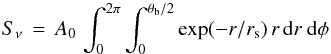 (A.1)where A0 is the brightness at the origin of the exponential, and r corresponds to the angular distance from the origin. Eq. (A.1) can be solved analytically to obtain:
 ![Mathematical equation: \appendix \setcounter{section}{1} \begin{equation} S_\nu\,=\,2\,\pi\,A_0\,\left \{ r_{\rm s}^2\, \left[ 1 - \exp \left( -\frac{\theta_{\rm b}}{2\,r_{\rm s}} \right)\right] - \frac{\theta_{\rm b}\,r_{\rm s}}{2} \exp \left( -\frac{\theta_{\rm b}}{2\,r_{\rm s}} \right) \right \}\cdot \label{eqn:exparea} \end{equation}](/articles/aa/full_html/2017/10/aa31000-17/aa31000-17-eq340.png) (A.2)The source FWHM θs is related to the exponential folding length by θs = 2rsln(2), obtained by calculating the diameter (i.e., twice the radius) at which the exponential distribution is equal to A0/ 2.
(A.2)The source FWHM θs is related to the exponential folding length by θs = 2rsln(2), obtained by calculating the diameter (i.e., twice the radius) at which the exponential distribution is equal to A0/ 2.
Flux corrections to a common beam size.
However, Eq. (A.1) is formally incorrect because of the need to convolve the pure exponential with the Gaussian beam when the exponential scale length rs is small relative to the beam radius θb/ 2. This convolution is given by the following, where we have taken advantage of the azimuthal symmetry and calculate the convolution along a single radial ray here given by x: 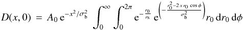 (A.3)where σb corresponds to the Gaussian σ assuming that the beam is Gaussian with FWHM θb (
 ).
).
Equation (A.3) can be integrated by separating the variables (r0, φ). After integrating in φ, we obtain: 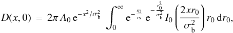 (A.4)where I0 is a modified Bessel function of the first kind. Eq. (A.4) can then be integrated numerically to obtain the surface brightness profile of the convolved exponential, as shown as the lower (red) dashed curves in Figs. A.1–A.4.
These figures show that for the four galaxies for which we were able to fit surface-brightness profiles and growth curves the pure exponential (2πA0 exp(−r/rs)) is equivalent to the integral given in Eq. (A.4) as long as the scale length rs is larger than θb/ 2. We thus fitted the growth curves with Eq. (A.2) in order to obtain the beam corrections. This is advantageous from a numerical point of view because otherwise it would be necessary to fit the growth curve to the integral of Eq. (A.4) which is in itself an integral.
To correct the fluxes (e.g., Sν in Jy), we scaled the observed dust fluxes to a common beam size of 22′′ by comparing the growth-curve integrals in the different beam sizes using the best-fit of the analytical formula in Eq. (A.2) to obtain rs and A0. We thus derive a multiplicative factor APcor as given in Col. (6) of Table A.1: S22 = SorigAPcor. We then apply the correction to velocity-integrated Tmb values by noting that S/ Ω = 2 kν2/c2 Tmb, where Ω is the beam solid angle, k is the Boltzmann constant, ν is the observed frequency, and c is the speed of light. Thus: 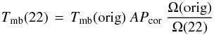 (A.5)where “orig” refers to the original values observed in the different beams. The flux and Tmb corrections necessary to convert our observations to a common beam size of 22′′ are given in Table A.1, together with the corrected velocity-integrated Tmb values that we use throughout the paper when we are examining line ratios (12CO(2–1)/12CO(1–0)) or fitting physical models. Corrected values are also reported in Tables 2–4 in the main text.
For Mrk 996 and NGC 7077, the only available cool dust images are from MIPS and, as mentioned above, the galaxies are not resolved. Thus, for these we assumed that the disk scale length rs is equal to 0.2 Ropt (optical radius from NED), consistently with Young et al. (1995), Leroy et al. (2009), Kuno et al. (2007) who all found that CO exponential scale lengths are, in the mean, equal to 1/5 the optical radius. This is also roughly consistent with the other four galaxies for which the mean rs/Ropt given by the best fits of the growth curves is 0.27 ± 0.16.
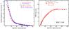 |
Fig. A.1 Left panel: PACS 160 μm radial surface brightness profile of NGC 1140; open (blue) circles give the profile obtained from azimuthally averaging the image, and filled (red) squares the analogous profile obtained from the first derivative of the photometric growth curve. The lower dashed curve show an exponential distribution of scale length 6.̋4 convolved with the PACS 160 μm beam (assuming it is Gaussian), and the upper one the same exponential but without convolution. Right panel: PACS 160 μm growth curve centered on the brightness peak. The left-most dotted vertical line gives the PACS beam radius (~5.̋5) and the right-most one the optical radius of NGC 1140 taken from NED (51′′). The solid grey curve corresponds to the best-fit exponential integral as described in the text. |
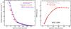 |
Fig. A.2 Left panel: PACS 160 μm radial surface brightness profile of NGC 3353 (Haro 3); open (blue) circles give the profile obtained from averaging the image over fixed-position-angle ellipses, and filled (red) squares the analogous profile obtained from the first derivative of the photometric growth curve. As in Fig. A.1, the dashed curves show the exponential convolved with the PACS 160 μm beam (lower), and the upper the exponential without convolution; the best-fit scale length is 5.̋0. Right panel: PACS 160 μm growth curve centered on the brightness peak. The left-most dotted vertical line gives the PACS beam radius (~5.̋5) and the right-most one the optical radius of NGC 3353 taken from NED (36′′). The solid grey curve corresponds to the best-fit exponential integral as described in the text; in the case of NGC 3353, the growth-curve best fit scalelength is slightly different from the radial profile one and we have adopted the growth-curve value for beam corrections. |
 |
Fig. A.3 Left panel: PACS 160 μm radial surface brightness profile of UM 448; open (blue) circles give the profile obtained from averaging the image over fixed-position-angle ellipses, and filled (red) squares the analogous profile obtained from the first derivative of the photometric growth curve. As in Fig. A.1, the dashed curves show the exponential convolved with the PACS 160 μm beam (lower), and the upper the exponential without convolution; the best-fit scale length is 4.̋0. Right panel: PACS 160 μm growth curve centered on the brightness peak. The left-most dotted vertical line gives the PACS beam radius (~5.̋5) and the right-most one the optical radius of UM 448 taken from NED (12′′). The solid grey curve corresponds to the best-fit exponential integral as described in the text; like NGC 3353, the growth-curve best fit scalelength for UM 448 is slightly different from the radial profile one and we have adopted the growth-curve value for beam corrections. |
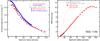 |
Fig. A.4 Left panel: MIPS 160 μm radial surface brightness profile of NGC 1156; open (blue) circles give the profile obtained from averaging the image over fixed-position-angle ellipses, and filled (red) squares the analogous profile obtained from the first derivative of the photometric growth curve. As in Fig. A.1, the dashed curves show the exponential convolved with the MIPS 160 μm beam (lower), and the upper the exponential without convolution; the best-fit scale length is 4.̋0. Right panel: MIPS 160 μm growth curve centered on the brightness peak. The left-most dotted vertical line gives the MIPS beam radius (~19′′) and the right-most one the optical radius of NGC 1156 taken from NED (99′′). The solid grey curve corresponds to the best-fit exponential integral as described in the text; like NGC 3353 and UM 448, the growth-curve best fit scalelength for NGC 1156 is slightly different from the radial profile one and we have adopted the growth-curve value for beam corrections. |
Appendix B: Gaussian beam size correction
To ensure that our results do not depend on the specific formulation of the correction for beam dilution, here we investigate a different assumption for the distribution of the CO emission, namely a Gaussian. For a Gaussian source distribution with a FWHM θs (corresponding to a Gaussian ![Mathematical equation: \hbox{$\sigma_{\rm s}\,=\,\theta_{\rm s}/ [2\,\sqrt{2\,\ln(2)}]$}](/articles/aa/full_html/2017/10/aa31000-17/aa31000-17-eq362.png) ), the integrated flux density within a beam with FWHM θb is given by the following integral (assuming azimuthal symmetry) in polar coordinates:
), the integrated flux density within a beam with FWHM θb is given by the following integral (assuming azimuthal symmetry) in polar coordinates: 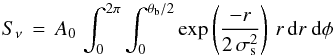 (B.1)where A0 is the normalization constant, and r corresponds to the angular distance from the origin. Equation (B.1) can be solved analytically to obtain:
 ![Mathematical equation: \appendix \setcounter{section}{2} \begin{equation} S_\nu\,=\,2\,\pi\,A_0\,\sigma_{\rm s}^2\, \left[ 1 - \exp \left( -\frac{\theta_{\rm b}^2}{8\,\sigma_{\rm s}^2} \right)\right] \cdot \label{eqn:exparea_gauss} \end{equation}](/articles/aa/full_html/2017/10/aa31000-17/aa31000-17-eq364.png) (B.2)However, like Eq. (A.1), Eq. (B.1) is formally incorrect because of the need to convolve the source Gaussian distribution with the Gaussian beam. This convolution is given by the following, where we have taken advantage of the azimuthal symmetry and calculate the convolution in Cartesian coordinates:
(B.2)However, like Eq. (A.1), Eq. (B.1) is formally incorrect because of the need to convolve the source Gaussian distribution with the Gaussian beam. This convolution is given by the following, where we have taken advantage of the azimuthal symmetry and calculate the convolution in Cartesian coordinates: 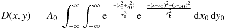 (B.3)where σb corresponds to the Gaussian σ assuming that the beam is Gaussian with FWHM θb (
 ).
).
It is straightforward to integrate Eq. (B.3) analytically to obtain: ![Mathematical equation: \appendix \setcounter{section}{2} \begin{equation} D(r)\,=\,A^\prime_0\,\frac{\sigma_{\rm s}^2}{(\sigma_{\rm b}^2 + \sigma_{\rm s}^2)}\,\exp \left[ \frac{-r^2}{(\sigma_{\rm b}^2 + \sigma_{\rm s}^2)} \right] \label{eqn:expconvolution_anal_gauss} \end{equation}](/articles/aa/full_html/2017/10/aa31000-17/aa31000-17-eq367.png) (B.4)where A0 has been substituted by the inclusion of the normalization constant of a two-dimensional Gaussian with integral unity,
(B.4)where A0 has been substituted by the inclusion of the normalization constant of a two-dimensional Gaussian with integral unity,  ; the independent Cartesian coordinates x and y have now been substituted with
  . Unlike Eq. (A.4) for the exponential source distribution, Eq. (B.4) can be easily
integrated to a circular aperture radius θb/ 2 to obtain the aperture correction: ![Mathematical equation: \appendix \setcounter{section}{2} \begin{eqnarray} S_\nu & = & A^\prime_0\,\frac{\sigma_{\rm s}^2}{(\sigma_{\rm b}^2 + \sigma_{\rm s}^2)}\ \int_0^{2\pi}\int_0^{\theta_{\rm b}/2} \exp\left( \frac{-r^2}{(\sigma_{\rm b}^2 + \sigma_{\rm s}^2)} \right)\, r \, {\rm d}r \ {\rm d}\phi \nonumber \\ & =& A^\prime_0\,\pi\,\sigma_{\rm s}^2\ \left[ 1 - \exp\left( {\frac{-\theta_{\rm b}^2}{4\,(\sigma_{\rm b}^2 + \sigma_{\rm s}^2)}} \right) \right] \cdot \label{eqn:expintegral_convolvedgauss} \end{eqnarray}](/articles/aa/full_html/2017/10/aa31000-17/aa31000-17-eq371.png) (B.5)For the case of a Gaussian source distribution, to correct the fluxes (e.g., Sν in Jy) to a common beam size, we scaled the observed CO fluxes by comparing the growth-curve integrals in the different beam sizes using the analytical formula in Eq. (B.5). Figure B.1 shows the aperture and the Tmb corrections for different transitions in the case of a Gaussian source distribution. Also shown are the exponentially-derived beam corrections for NGC 1140 (see Appendix A).
(B.5)For the case of a Gaussian source distribution, to correct the fluxes (e.g., Sν in Jy) to a common beam size, we scaled the observed CO fluxes by comparing the growth-curve integrals in the different beam sizes using the analytical formula in Eq. (B.5). Figure B.1 shows the aperture and the Tmb corrections for different transitions in the case of a Gaussian source distribution. Also shown are the exponentially-derived beam corrections for NGC 1140 (see Appendix A).
Flux corrections to a common beam size.
In the best-fit procedure described in the main text, we sample source FWHM θs ranging from 2′′ to 40′′ with steps of 1′′, and for each of these derive a multiplicative factor APcorS22 = Sorig APcor (see Eq. (A.5)). We then apply this correction to velocity-integrated Tmb values, and consider the best fit as the one with the lowest χ2 value. Corrected values for NGC 1140 are given in Table B.1.
It is interesting that the Gaussian beam corrections found by the χ2 minimization technique are the same as the independently-derived exponential beam corrections. It seems unlikely that this is a fortuitous result, but rather that it is confirming the validity of either approach to beam corrections.
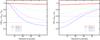 |
Fig. B.1 Left panel: (inverse of) aperture corrections as given in Eq. (B.5) plotted against Gaussian source FWHM θs. Right panel: Tmb corrections (APcorplotted against θs. In both panels, different 12CO beams are shown by different colors as line types as described in the legend: 12CO(1–0): solid (red); 12CO(2–1): dashed (blue); 12CO(3–2): dotted (green); 12CO(4–3): dot-dashed (purple). The horizontal (light-weighted) lines of the same type correspond to the exponentially-derived quantities for aperture (left panel) and Tmb corrections (right) for NGC 1140. They converge roughly to a common Gaussian beam size of θs ~ 26′′ (see main text for more details). |
All Tables
All Figures
|
Fig. 1 Various 12CO transitions for Mrk 996, NGC 3353, NGC 7077, NGC 1156, and UM 448. Top row: 12CO(1–0), 12CO(2–1) (IRAM), and 12CO(2–1) (APEX) for Mrk 996; second row: 12CO(1–0) for NGC 3353 (Haro 3) for three pointings ([0, 0], [0, +10′′], [−6′′, −9′′]); third row: 12CO(2–1) for NGC 3353 (Haro 3) for three pointings; fourth row: 12CO(1–0), 12CO(2–1) (IRAM), and 12CO(3–2) (APEX) for NGC 7077 (Mrk 900); fifth row: 12CO(1–0) for NGC 1156 and UM 448, and 12CO(2–1) (APEX) for UM 448; bottom row: 12CO(2–1) (IRAM) for NGC 1156 and UM 448 and 12CO(3–2) (APEX) for UM 448. The baselines are shown as a horizontal solid line, together with the multiple-component Gaussian fits as described in Sect. 3.3. The vertical axes are in |
| In the text | |
|
Fig. 2 12CO, 13CO, and [Ci](1–0) transitions for NGC 1140. Top row: 12CO(1–0), 12CO(2–1) (IRAM), and 12CO(3–2) (APEX); second row: 13CO(1–0), 13CO(2–1) (IRAM), and 12CO(4–3) (APEX); third row: [Ci](1–0) (APEX). As in Fig. 1, the baselines are shown as a horizontal solid line, together with the multiple-component Gaussian fits as described in Sect. 3.3. The vertical axes are in |
| In the text | |
|
Fig. 3 Histogram of observed 12CO(2–1)/12CO(1–0) line ratios for our targets corrected for beam dilution as described in Sect. 4. Because of the larger beam, for Mrk 996 and UM 448, we show the APEX 12CO(2–1) measurements rather than the ones from IRAM. Also plotted are the line ratios corrected for beam dilution of a large sample of spiral galaxies observed by Braine & Combes (1992). |
| In the text | |
|
Fig. 4 Histogram of observed 12CO(3–2)/12CO(1–0) line ratios for our targets. Also shown are the line ratios for a large sample of galaxies observed by Mao et al. (2010). Neither set of observations has been corrected for beam dilution; see Sect. 5.2 for more discussion. |
| In the text | |
|
Fig. 5 Beam-corrected [Ci]/12CO(1–0) line ratios for NGC 1140 and galaxies from the literature plotted against oxygen abundance 12 + log(O/H). The solid line corresponds to the data regression by Bolatto et al. (2000a), and the dashed one to the PDR model by Bolatto et al. (1999). Beam dilution has been corrected for as described in Sect. 4. |
| In the text | |
|
Fig. 6 HCN luminosity plotted against FIR luminosity, LFIR (left panel) and CO(1–0) luminosity, |
| In the text | |
|
Fig. 7 CO(3-2) luminosity, |
| In the text | |
|
Fig. 8 Rotation or population level diagram for NGC 1140. A beam correction has been applied to the integrated intensities (see Sect. 4 for more details). Both 12CO and 13CO transitions are shown, as indicated by open (red) circles and filled (blue) squares, respectively. The gray dashed line for 12CO corresponds to the best-fit regressions; the temperature for 13CO is ill determined with only two transitions, so we fixed it to the 12CO value of Tex = 18.1 K. |
| In the text | |
|
Fig. 9 Rotation or population level diagram for UM 448 and NGC 7077. A beam correction has been applied to the integrated intensities (see Sect. 4 for more details). The gray dashed line corresponds to the best-fit regression; as shown by the legend, the galaxies are differentiated by different symbols for 12CO emission (open (orange) circles and filled (green) circles, for UM 448 and NGC 7077, respectively). |
| In the text | |
|
Fig. 10 RADEX models (with ΔV = 20 km s-1) of 12CO line ratios plotted against Tkin: the left panel shows 12CO(2–1)/12CO(1–0) and the right 12CO(3–2)/12CO(1–0). The observations of NGC 1140, shown as a (black) filled circle, have been corrected for beam dilution assuming an exponential source distribution as described in Sect. 4 (see also Figs. 3 and 4). The approximate best-fit RADEX model for NGC 1140 (see Sect. 7.3) is shown in both panels as (purple) solid curves that coincide very well with the observations of NGC 1140. Also shown are three additional parameter combinations of 12CO column density N12CO and volume density nH2. The R31 parameter space occupied by the other galaxies (like Fig. 4, no beam corrections) is shown in the right-hand panel as a hatched region and solid horizontal lines (NGC 7077, UM 448, and an upper limit for Mrk 996). |
| In the text | |
|
Fig. 11 RADEX fit χ2 surface (for the “Set 1” line ratios) with the exponential beam correction as a function of Tkin and nH2 in the left panel, and as a function of N12CO and τ(12CO(1–0)) in the right. The RADEX models shown here have ΔV = 20 km s-1. The associated χ2 values are shown as a side-bar color table. The χ2 color table in the right panel is different from the left because the interpolation used for the graphic display suffers from the coarser resolution in column density. The best-fit values are shown as an open (white) circle; the error bars shown consider a slightly more limited range in χ2 respect to Table 6. |
| In the text | |
|
Fig. 12 RADEX fit χ2 surface (for the “Set 1” line ratios, assuming the Gaussian-derived beam correction factors) as a function of N12CO and Gaussian FWHM θs in the left panel, The RADEX models shown here have ΔV = 20 km s-1; the associated χ2 values are shown as a side-bar color table. The best-fit values are shown as an open (white) circle; the error bars shown consider a slightly more limited range in χ2 respect to Table 6. |
| In the text | |
|
Fig. 13 RADEX best-fit model compared to observations for the CO excitation ladder of NGC 1140; the observations have been corrected for beam size as described in Sect. 4, and normalized to the CO(1–0) flux. The observations are shown as filled blue circles (12CO) and red squares (13CO), and the range of the allowed RADEX models by the light-blue region (for 12CO); 13CO points have arbitrarily offset relative to 12CO for clarity. The dashed curve shows the ν2 behavior (here normalized to J = 1) expected for optically-thick emission. |
| In the text | |
|
Fig. 14 RADEX fit of the χ2 (logarithmic) surface of the [Ci]/12CO fits as a function of nH2 and NCI(1−0); the left panel shows the intensity fits (Eq. (4)) and the right the ratio ones (Eq. (5)). The RADEX models shown here have ΔV = 20 km s-1. The associated Log(χ2) values are shown as a side-bar color table. The best-fit values are shown as an open (white) circle; the error bars shown consider a slightly more limited range in χ2 respect to Table 6. |
| In the text | |
|
Fig. 15 RADEX models of HCN(1–0)/12CO(1–0) line ratios plotted against nH2, and assuming [CO]/[HCN] = 105. Here the ΔV = 20 km s-1 models are illustrated. The upper limit HCN(1–0)/12CO(1–0) ratio for NGC 1140, shown as a (black) filled circle, has not been corrected for beam dilution because of the similar beam sizes for the two transitions. The approximate best-fit RADEX model for NGC 1140 is shown as a (purple) solid curve that is consistent with the non-detection of HCN(1–0). Also shown are three additional parameter combinations of 12CO column density N12CO and volume density nH2. |
| In the text | |
|
Fig. 16 12CO/13CO abundance ratio plotted against N(12CO). The shaded rectangle shows the ranges of values from RADEX fits (ΔV = 20 km s-1) of NGC 1140. The solid line corresponds to the models of the 12CO/13CO abundance ratio vs. the 12CO column density by Szűcs et al. (2014). The error bars for these models (vertical black lines) are (very roughly) estimated from their Fig. 8. |
| In the text | |
|
Fig. A.1 Left panel: PACS 160 μm radial surface brightness profile of NGC 1140; open (blue) circles give the profile obtained from azimuthally averaging the image, and filled (red) squares the analogous profile obtained from the first derivative of the photometric growth curve. The lower dashed curve show an exponential distribution of scale length 6.̋4 convolved with the PACS 160 μm beam (assuming it is Gaussian), and the upper one the same exponential but without convolution. Right panel: PACS 160 μm growth curve centered on the brightness peak. The left-most dotted vertical line gives the PACS beam radius (~5.̋5) and the right-most one the optical radius of NGC 1140 taken from NED (51′′). The solid grey curve corresponds to the best-fit exponential integral as described in the text. |
| In the text | |
|
Fig. A.2 Left panel: PACS 160 μm radial surface brightness profile of NGC 3353 (Haro 3); open (blue) circles give the profile obtained from averaging the image over fixed-position-angle ellipses, and filled (red) squares the analogous profile obtained from the first derivative of the photometric growth curve. As in Fig. A.1, the dashed curves show the exponential convolved with the PACS 160 μm beam (lower), and the upper the exponential without convolution; the best-fit scale length is 5.̋0. Right panel: PACS 160 μm growth curve centered on the brightness peak. The left-most dotted vertical line gives the PACS beam radius (~5.̋5) and the right-most one the optical radius of NGC 3353 taken from NED (36′′). The solid grey curve corresponds to the best-fit exponential integral as described in the text; in the case of NGC 3353, the growth-curve best fit scalelength is slightly different from the radial profile one and we have adopted the growth-curve value for beam corrections. |
| In the text | |
|
Fig. A.3 Left panel: PACS 160 μm radial surface brightness profile of UM 448; open (blue) circles give the profile obtained from averaging the image over fixed-position-angle ellipses, and filled (red) squares the analogous profile obtained from the first derivative of the photometric growth curve. As in Fig. A.1, the dashed curves show the exponential convolved with the PACS 160 μm beam (lower), and the upper the exponential without convolution; the best-fit scale length is 4.̋0. Right panel: PACS 160 μm growth curve centered on the brightness peak. The left-most dotted vertical line gives the PACS beam radius (~5.̋5) and the right-most one the optical radius of UM 448 taken from NED (12′′). The solid grey curve corresponds to the best-fit exponential integral as described in the text; like NGC 3353, the growth-curve best fit scalelength for UM 448 is slightly different from the radial profile one and we have adopted the growth-curve value for beam corrections. |
| In the text | |
|
Fig. A.4 Left panel: MIPS 160 μm radial surface brightness profile of NGC 1156; open (blue) circles give the profile obtained from averaging the image over fixed-position-angle ellipses, and filled (red) squares the analogous profile obtained from the first derivative of the photometric growth curve. As in Fig. A.1, the dashed curves show the exponential convolved with the MIPS 160 μm beam (lower), and the upper the exponential without convolution; the best-fit scale length is 4.̋0. Right panel: MIPS 160 μm growth curve centered on the brightness peak. The left-most dotted vertical line gives the MIPS beam radius (~19′′) and the right-most one the optical radius of NGC 1156 taken from NED (99′′). The solid grey curve corresponds to the best-fit exponential integral as described in the text; like NGC 3353 and UM 448, the growth-curve best fit scalelength for NGC 1156 is slightly different from the radial profile one and we have adopted the growth-curve value for beam corrections. |
| In the text | |
|
Fig. B.1 Left panel: (inverse of) aperture corrections as given in Eq. (B.5) plotted against Gaussian source FWHM θs. Right panel: Tmb corrections (APcorplotted against θs. In both panels, different 12CO beams are shown by different colors as line types as described in the legend: 12CO(1–0): solid (red); 12CO(2–1): dashed (blue); 12CO(3–2): dotted (green); 12CO(4–3): dot-dashed (purple). The horizontal (light-weighted) lines of the same type correspond to the exponentially-derived quantities for aperture (left panel) and Tmb corrections (right) for NGC 1140. They converge roughly to a common Gaussian beam size of θs ~ 26′′ (see main text for more details). |
| In the text | |
Current usage metrics show cumulative count of Article Views (full-text article views including HTML views, PDF and ePub downloads, according to the available data) and Abstracts Views on Vision4Press platform.
Data correspond to usage on the plateform after 2015. The current usage metrics is available 48-96 hours after online publication and is updated daily on week days.
Initial download of the metrics may take a while.