| Issue |
A&A
Volume 606, October 2017
|
|
|---|---|---|
| Article Number | A35 | |
| Number of page(s) | 8 | |
| Section | Interstellar and circumstellar matter | |
| DOI | https://doi.org/10.1051/0004-6361/201630187 | |
| Published online | 04 October 2017 | |
Evidence for disks at an early stage in class 0 protostars?⋆
1 LERMA, Observatoire de Paris, PSL Research University, CNRS, École Normale Supérieure, Sorbonne Universités, UPMC Univ. Paris 06, 75005 Paris, France
e-mail: This email address is being protected from spambots. You need JavaScript enabled to view it.
2 Institut de Radioastronomie Millimétrique (IRAM), 300 rue de la Piscine, 38406 Saint-Martin d’ Hères, France
3 Univ. Lyon, ENS de Lyon, Univ. Lyon1, CNRS, Centre de Recherche Astrophysique de Lyon, UMR 5574, 69007 Lyon, France
4 Observatorio Astronómico Nacional (OAN, IGN), Apdo 112, 28803 Alcalá de Henares, Spain
5 Instituto de Ciencia de Materiales de Madrid (ICMM-CSIC), 28049 Cantoblanco, Madrid, Spain
6 LERMA, Observatoire de Paris, PSL Research University, CNRS, Sorbonne Universités, UPMC Univ. Paris 06, 75014 Paris, France
7 National Radio Astronomy Observatory, 520 Edgemont Road, Charlottesville, VA 22903, USA
8 LERMA, Observatoire de Paris, PSL Research University, CNRS, Sorbonne Universités, UPMC Univ. Paris 06, École Normale Supérieure, 92190 Meudon, France
9 Laboratoire d’Astrophysique de Bordeaux, Univ. Bordeaux, CNRS, B18N, allée Geoffroy Saint-Hilaire, 33615 Pessac, France
Received: 3 December 2016
Accepted: 21 August 2017
Abstract
Aims. The formation epoch of protostellar disks is debated because of the competing roles of rotation, turbulence, and magnetic fields in the early stages of low-mass star formation. Magnetohydrodynamics simulations of collapsing cores predict that rotationally supported disks may form in strongly magnetized cores through ambipolar diffusion or misalignment between the rotation axis and the magnetic field orientation. Detailed studies of individual sources are needed to cross check the theoretical predictions.
Methods. We present 0.06–0.1′′ resolution images at 350 GHz toward B1b-N and B1b-S, which are young class 0 protostars, possibly first hydrostatic cores. The images have been obtained with ALMA, and we compare these data with magnetohydrodynamics simulations of a collapsing turbulent and magnetized core.
Results. The submillimeter continuum emission is spatially resolved by ALMA. Compact structures with optically thick 350 GHz emission are detected toward both B1b-N and B1b-S, with 0.2 and 0.35′′ radii (46 and 80 au at the Perseus distance of 230 pc), within a more extended envelope. The flux ratio between the compact structure and the envelope is lower in B1b-N than in B1b-S, in agreement with its earlier evolutionary status. The size and orientation of the compact structure are consistent with 0.2′′ resolution 32 GHz observations obtained with the Very Large Array as a part of the VANDAM survey, suggesting that grains have grown through coagulation. The morphology, temperature, and densities of the compact structures are consistent with those of disks formed in numerical simulations of collapsing cores. Moreover, the properties of B1b-N are consistent with those of a very young protostar, possibly a first hydrostatic core. These observations provide support for the early formation of disks around low-mass protostars.
Key words: stars: formation / ISM: clouds / submillimeter: ISM / ISM: individual objects: Barnard 1b / ISM: molecules
The reduced images and datacubes are only available at the CDS via anonymous ftp to cdsarc.u-strasbg.fr (130.79.128.5) or via http://cdsarc.u-strasbg.fr/viz-bin/qcat?J/A+A/606/A35
© ESO, 2017
1. Introduction
A key issue in the early stages of star formation is the formation epoch of a rotationally supported disk, which mediates the accretion onto the forming star and evolves into a protoplanetary disk at later stages. Analytical and numerical studies have shown that the formation of a rotationally supported disk requires leaving enough angular momentum during the collapse. This can be a problem when a magnetic field is present because the field can efficiently transport angular momentum and prohibits the formation of a disk (e.g., Hennebelle & Fromang 2008). Earlier theoretical studies were mostly restricted to the simple case of a magnetic field parallel to the rotation axis, a configuration where magnetic braking can be very efficient and quench the formation of a disk. The B335 protostar seems to be the best case of such a geometry (Yen et al. 2015). The occurrence frequency of such systems is unknown, however. They may be the exception rather than the rule, since Lee et al. (2016) have shown that outflow axes of wide binary or multiple systems are not aligned in Perseus, suggesting that these systems are formed in more complex configurations. Different effects contribute to reducing the efficiency of magnetic braking and allowing early formation of disks: a rotation axis not aligned with the magnetic field (Ciardi & Hennebelle 2010), the level of turbulence (Joos et al. 2013), or deviations from ideal magnetohydrodynamics (MHD), especially the role of ambipolar diffusion (Tomida et al. 2015; Masson et al. 2016; Zhao et al. 2016; Hennebelle et al. 2016).
Disks have been commonly found around class I protostars and class II sources (Williams & Cieza 2011; Harsono et al. 2014), but their presence around younger objects, especially class 0 protostars, is still debated. Establishing the presence of rotationally supported disks in class 0 protostars (defined as protostars with a high ratio of the submillimeter to the bolometric luminosity; André et al. 1993) is especially important because objects at this stage are accreting material from their surrounding envelope at the highest rate. Therefore these objects are best suited for a comparison with theoretical collapse models, especially regarding the question of the complex interplay of velocity field and magnetic field on the final structure of the environment of the forming star. The number of such protostars that can be studied in detail is limited, and direct high angular resolution imaging in the near-infrared is often impossible because of the very high column densities of dust and gas in the surrounding envelopes. Only (sub)millimeter interferometers have the sensitivity and angular resolution to detect circumstellar material. Maury et al. (2010) performed a pilot study of multiplicity with the IRAM-PdBI at ~0.4′′ resolution that showed a low multiplicity fraction at small separations. At the achieved angular resolution, the class 0 protostars are detected, but the structure of the millimeter emission is not resolved. The young protostars B1b-S and B1b-N are promising objects for studying the early stages of low-mass star formation. These sources are located in the Barnard 1b core of the Barnard 1 dark cloud, a moderately active star-forming region in the Perseus molecular cloud at a distance of 230 pc (Hirota et al. 2008). The analysis of the spectral energy distribution (SED) based on Herschel and Spitzer data performed by Pezzuto et al. (2012) shows that both sources have low infrared luminosities (Lbol = 0.1 L⊙ for B1b-N, Lbol = 0.3 L⊙ for B1b-S), with the SED peaking longward of 100 μm. To further progress in the understanding of the nature of these sources and their relation to their parental core, Hirano & Liu (2014) obtained CO (J = 2 → 1), 13CO (J = 2 → 1) and H13CO+ (J = 1 → 0) observations with the SMA, which showed that both B1b-S and B1b-N are driving low-velocity molecular outflows. The continuum sources are largely unresolved down to an angular resolution of 0.5′′ at 7 mm wavelength (Hirano & Liu 2014). Huang & Hirano (2013) showed that N2H+ (J = 3 → 2) and N2D+ (J = 3 → 2) present a compact emission component associated with the continuum sources, together with extended emission in the surrounding envelope. The high intensity of these high-dipole moment species has been interpreted by Daniel et al. (2013) using a sophisticated radiative transfer code. As expected for a cold and dense region, the deuterium fractionation clearly increases with the density, although the absolute abundances slowly decrease. Using NOEMA with a 2.3′′ beam, Gerin et al. (2015) further confirmed the presence of slow molecular outflows driven by B1b-N and B1b-S, and determined the outflow dynamical times, masses, mechanical luminosities, and mass-loss rates. They concluded that the two sources are at most a few thousand years old, and that the properties of B1b-N are consistent with those of a first hydrostatic core (FHSC). The outflows are launched in different directions, which is probably a consequence of the high degree of turbulence in the Barnard 1b core, which is impacted by outflows from nearby young stellar objects (YSOs; Hirano & Liu 2014). So far, the inner structure of the compact components of B1b-N and B1b-S remained unresolved or only marginally resolved. Because these sources are young and the physical and chemical structure of the Barnard 1b core are well known (see the recent analysis of the depletion and ionization rate by Fuente et al. 2016), it is interesting to probe these sources in more detail, as a means to constrain current theoretical understanding of low-mass star formation.
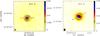 |
Fig. 1 Continuum emission at 349 GHz toward B1b-N (left) and B1b-S (right). The gray contours show the 32 GHz continuum emission from the VANDAM survey (Tobin et al. 2015, 2016) and are drawn at 0.05, 0.1, 0.2, 0.3, 0.4, and 0.5 mJy/beam. The ALMA and VLA beam sizes are shown as black and gray ellipses. The red and blue arrows show the approximate direction of the outflows. |
Summary of combined observations.
2. ALMA observations
We present ALMA Cycle 3 observations, performed on 2015 November 22 during the Long Baseline Campaign, combined with supplementary Director’s Discretionay Time (DDT) observations obtained on 2016 June 16. For the first data set, a total of 46 antennas were used in the C36-7 configuration, with baselines from 82 m up to 15 km (projected on source), providing an angular resolution of ~0.06′′, corresponding to ~13 au at the distance of Perseus, 230 pc. Four continuum base-bands with 2 GHz bandwidth, 128 channels, and dual polarization received the digitized signals from the Band 7 receiver. Central sky frequencies in each band are 336.5 and 338.4 GHz in the lower sideband (LSB), and 348.5 and 350.5 GHz in the upper sideband (USB). The channel spacing is 15.6 MHz, resulting in a spectral resolution of ~27 km s-1 (Hanning smoothed). Imaging with the first dataset revealed artifacts attributable to a lack of shorter spacings. For the second data set, a total of 38 antennas were used in the C40-4 configuration with baselines from 15 m to 704 m. The setups were otherwise identical.
Observations for both datasets were obtained in single sessions, providing 30 min on source combined. The two fields B1b-N and B1b-S were observed alternately for 55 s each, with a phase calibrator scan in between, observed for 20 s. The phase calibrator was J0336+3218, located at an angular separation of ~1.36° from the B1b cores. A second calibrator (J0359+3220, located at 5.7° distance), observed every 5 min, was also included in order to check the quality of the phase transfer (see Appendix A for more information). Standard calibration was performed in CASA 4.5.0, while for imaging and data analysis we used the GILDAS software and CASA 4.7.0. For the first dataset, two other quasars were used for flux (J0238+1636) and bandpass (J0237+2848) calibration. The adopted flux density of J0238+1636 is 1.06 Jy at 343.5 GHz. For the second dataset, Ceres was observed for flux calibration and J0237+2848 for bandpass calibration. J0238+1636 and J0237+2848 are both among the regularly monitored ALMA calibrators, and the obtained fluxes are consistent with the data in the ALMA Calibrator Database. For the DDT observations, the Ceres data could not be used for flux calibration and J0237+2848 (flux 1.10 Jy at 343.5 GHz) was used instead. Weather conditions were good and appropriate for Band 7 observations, with a precipitable water vapor of 0.8 (0.7) mm and a median system temperature of 170 (160) K for the long-baseline (DDT) sessions.
The flux calibration we achieved is very good, with the curves of flux versus uv distance overlapping for the two program sources, as illustrated in Fig. A.2 (although the gain calibrator’s flux varied somewhat). Extended flux is clearly present for both sources, as the recovered flux increases with decreasing baseline length. Spectral windows for each sideband were averaged for the combined data.
For the high-resolution data, the final clean beam is 0.064′′ × 0.048′′ at PA 168° with a noise level of 0.1 mJy/beam for each spectral window, corresponding to about 0.35 K in the LSB and 0.32 K in the USB. For the DDT data, the final clean beam is 0.39′′ × 0.27′′ at PA − 9.9°, with a noise level of 0.2 mJy/beam, corresponding to about 18 mK.
We have checked that all spectral windows are free of strong line emission. With the typical line widths in Barnard 1b of ~1 km s-1, which can increase to ~5 km s-1 when line wings are present, line emission will be diluted in the broad spectral channels used for continuum observations. Although we cannot exclude some line contamination, we are confident that the contribution of spectral lines to the detected continuum fluxes remains modest.
For the data reported here, we have concatenated the two datasets. The final clean beams are 0.086′′ × 0.069′′ for B1b-N, and 0.14′′ × 0.11′′ for B1b-S. We averaged the two spectral windows of each sideband to obtain the final images.
3. Results
3.1. Resolving the B1b-N and B1b-S continuum emission
The ALMA images are displayed in Fig.1, while Table 1 presents a summary of the observations. For each source we show as gray contours the 32.9 GHz emission mapped with a 0.2′′ beam with the Very Large Array (VLA) as a part of the VLA Nascent Disk and Multiplicity Survey of Perseus Protostars (VANDAM; Tobin et al. 2015, 2016). ALMA clearly resolves a compact slightly elongated structure toward both sources that is located within a more extended region of faint emission.
We list in Table 1 the values of flux densities at the peak and within a 1′′ radius (230 au). While both sources reach similar intensities at large scale, the compact component in the youngest source B1b-N is smaller and represents a smaller fraction of the total flux than for the slightly more evolved source B1b-S. The high flux densities of the compact components toward B1b-N and B1b-S, >10 mJy/beam, correspond to a brightness temperature of ~35 K, comparable to the expected gas and dust temperatures in these sources (Commerçon et al. 2012a). It is therefore likely that the continuum emission of the compact component is optically thick.
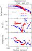 |
Fig. 2 Fit parameters of intensity isocontours using ellipses. B1b-N data are shown in blue and B1b-S data in red. The top panel presents the variation of the major and minor axis sizes. The middle panel shows the ellipse position angle, PA, and the bottom panel the ellipticity, e = 1 − Rmin/Rmaj. The beam profiles are displayed in the top panel. The beam position angles and ellipticities are 1.1° and 0.2 for B1b-N and 16° and 0.21 for B1b-S. The upper scale displays the correspondence between antenna baseline and angular scale. |
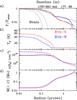 |
Fig. 3 Panel a: distribution of the circularly averaged specific intensity normalized to the peak value as a function of radius toward B1b-S and B1b-N. The gray lines show the analytical fits and the dotted lines the beam profiles. The upper scale presents the baseline in meters corresponding to the angular scale. Data for B1b-N are displayed in blue and data for B1b-S in red. Panel b: dust temperature (Td) radial distribution, assuming that the 350 GHz emission is optically thick, with a minimum value set to 12 K. Panel c: molecular hydrogen density, using the derived Td and assuming optically thin emission. This represents a lower limit to the real density. The dashed lines show the densities, assuming a constant value of the dust temperature. Panel d: cumulative mass distribution obtained by combining the information at 350 and 32 GHz. |
To obtain further insight into the spatial distribution of the emission, we fit the flux density isocontours with ellipses centered on the protostar positions, with the position angle (PA) and ellipticity as free parameters. These fits are illustrated in Fig. 2 with B1b-N data in blue and B1b-S data in red. We also used simple Gaussian profiles to determine the source sizes and shapes, and compared these estimates with the core sizes obtained by fitting the circularly averaged intensity profiles as described in Appendix B. Table 2 lists the sizes and PAs of the central sources. We obtain a FWHM of about 0.4′′, corresponding to ~90 au at the Perseus distance. The sizes of the compact component for both sources correspond to the size of the centimeter continuum emission, as illustrated in Fig. 1. The similarity between the submillimeter and centimeter images, and the low spectral index  between 32 and 350 GHz of 2.4 and 2.8 for B1b-N and B1b-S, respectively, confirm the high opacity of the 350 GHz emission. It is remarkable that B1b-N is weaker than B1b-S at wavelengths shorter than about 3 mm, but becomes stronger for longer wavelengths (Gerin et al. 2015). This behavior is explained by a larger part of the total flux coming from the compact source at long wavelengths and the shallower spectral index of this compact component as compared with that of the extended envelope. Such a shallow spectral index down to at least 32 GHz is consistent with either very high opacities even at 32 GHz or the presence of large grains with a significantly higher emissivity at 32 GHz than standard interstellar grains. Studies of the submillimeter (Chen et al. 2016) and mid-infrared emission (Lefèvre et al. 2014) have shown that large dust grains are present in Barnard 1b, as testified by the high portion of “transitional β”1 values, and the coreshine phenomenon. With a standard grain population, the dust opacity at 350 GHz is a factor 50–100 higher than at 32 GHz. High opacity at 32 GHz therefore requires extreme column densities, of N(H2) ~ 1027 cm-2, and mean H2 densities higher than ~1012 cm-3 at the 0.2′′ scale. We therefore propose that both phenomena contribute to the flattening of the spectral index, the high opacity of the continuum emission at 350 GHz and the presence of large dust grains.
3.2. Analysis of intensity, density, and temperature radial distributions
Figure 3 presents the observed distributions of the circularly averaged specific intensity as a function of the angular radius for B1b-N and B1b-S and their associated fits in the top panel, together with the variations of dust temperature, molecular hydrogen density, and the cumulative gas masses in the other panels. While the dust continuum emission from the compact component (disk) is probably optically thick, the sharp decrease in flux densities outside the central component indicates that the opacity of the dust thermal emission drops. The assumption of optically thin emission is therefore likely valid for the envelope region. Using the procedure outlined in Appendix B, we derived the radial distribution of the gas density. This assumes spherical symmetry, that the gas is molecular, and that the dust has constant optical properties, 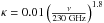 cm2 g-1, a value commonly used for cold and dense cores, from Ossenkopf & Henning (1994), which is close to the composite aggregate disk opacities computed by Semenov et al. (2003). A further assumption is the good thermal coupling of the dust and gas, which leads to equal gas and dust temperatures, supported by the high densities encountered in the cores (n(H2) > 105 cm-3, Daniel et al. 2013). Finally, we used a simple equation of state to relate the dust temperature and the gas density: i) the gas is isothermal and the kinetic temperature T0 is 12 K (derived by Lis et al. 2010, from NH3) for all densities lower than a density threshold n0(H2) = 1010 cm-3; ii) the gas follows a polytropic equation of state for densities higher than n0(H2), with an exponent γ, implying
 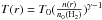 . We have chosen γ = 1.6, adapted for moderately warm molecular gas. For the “disk region” within a radius of 0.3′′, we derived the dust temperature directly from the brightness temperatures. As the 350 GHz emission is optically thick, we used the 32 GHz flux densities to determine the gas masses, assuming an emissivity of κ = 0.006 cm2 g-1 at 1 cm, adapted to a population of large grains with sizes reaching 3 mm (Tazzari et al. 2016), and using the temperature determined from the 350 GHz data. The total masses were derived by combining the determinations at 32 GHz and at 350 GHz.
Analytical fits and physical structure.
The parameters used for the fit and the resulting physical conditions are given in Table 2. For both sources, we used a two-component fit with a central component with a steep flux density profile (r-4 or r-6) and a more extended envelope with flux decreasing as r-2. Because of the lack of short spacings, some flux may be missing at scales larger than ~2′′. Therefore the parameters of the second component are not well constrained. The exponent and size scale should not be considered as having a physical meaning, but only as a convenient mathematical description of the observed data. Assuming optically thin 350 GHz emission, the maximum H2 density reached in the central region is about 1010 cm-3 for both sources. The true densities are expected to be significantly higher. The peak dust temperature is 40 and 60 K, somewhat higher than the mean temperature used for the SED fit by Hirano & Liu (2014, 16 and 18 K for B1b-N and B1b-S), but still consistent with faint emission at wavelengths shorter than 70 μm. For both sources, the warm region where the dust temperature is higher than 12 K is fairly small, less than 0.3′′ in radius. The cumulative mass distributions show that the sources may still be accreting, since a large part of the core mass is located at radii larger than 0.3′′. B1b-S is more condensed and presents a steeper increase in mass with radius than B1b-N, supporting its more evolved classification (established from the larger extent of its molecular outflow and warmer SED; Gerin et al. 2015). The mass of the compact component is at least 0.1 M⊙ for both B1b-N and B1b-S, given our hypothesis on the dust grain emissivity at 32 GHz.
To check whether the compact component detected with ALMA could simply represent the inner region of a protostellar envelope, we compared the cumulative flux distribution of a simple isothermal spherical envelope model with that of B1b-N and B1b-S. We used a density profile  , where r is the radius in arcseconds, a uniform temperature of 12 K, and the dust emissivity law described above. These parameters lead to a predicted flux in a 20′′ beam of about 2 Jy, comparable to the measured flux density of B1b-N and B1b-S with SCUBA, about 3 Jy (Pezzuto et al. 2012; Hirano & Liu 2014; I-Hsiu Li et al. 2017), and a high opacity of the central region within a radius of 0.1 arcsec, as illustrated in Fig. 4.
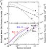 |
Fig. 4 Top panel: variation with radius of the molecular hydrogen density, n (dash-dotted line), the column density, N (dotted line), and the resulting continuum opacity at 350 GHz, τ (solid line) for a simple spherical isothermal (12 K) core model. Bottom panel: variation of the gas mass (dash-dotted line) and 350 GHz flux (solid line) as a function of radius for the model displayed in the top panel. The dashed gray line shows the expected cumulative flux distribution for a pure blackbody (optically thick emission) at the same temperature. The observed data toward B1b-N and B1b-S are displayed in blue and red, respectively, including the ALMA data from 0.05′′ to 3′′ and JCMT and SMA data between 3′′ and 12′′ (Pezzuto et al. 2012; Hirano & Liu 2014; I-Hsiu Li et al. 2017). |
However, this model presents a cumulative flux distribution very different from that of B1b-N and B1b-S, which have a more spatially extended region of high opacity and a higher temperature, supporting the association of the compact component detected with ALMA with a disk. To further understand the nature of this compact component, we have used numerical simulations of collapsing cores.
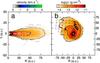 |
Fig. 5 Cross section of the 3D numerical simulations showing the structure of the protostellar disk. The colors show the density field and the arrows the velocity vectors. Panel a: an edge-on view (azimuthal mean) and panel b: a face-on view of all cells that satisfy the criteria for a rotationally supported disk (Joos et al. 2012). |
4. 3D collapse model and comparison with the ALMA data
4.1. Description of the model
In this section, we compare our ALMA data with simulated observations obtained by post-processing a 3D numerical simulation from Hennebelle et al. (2016). We have used the RAMSES code (Teyssier 2002), which integrates the MHD equations using a constrained transport scheme (Fromang et al. 2006; Teyssier et al. 2006) and accounts for the ambipolar diffusion (Masson et al. 2012). The model is almost identical to the model used in Masson et al. (2016), except that we account for initial turbulent velocity fluctuations instead of a coherent global solid body rotation (e.g., Joos et al. 2013). The model consists of a collapsing 1 M⊙ magnetized and turbulent dense core of radius R0 = 2500 au. The initial dense core density and temperature are uniform, ρ0 = 9.4 × 10⁻¹⁸ g cm-3 corresponding to n(H2) = 2.4 × 106 cm-3 and T = 10 K. The corresponding ratio between the thermal energy and the gravitational energy is αth = 0.25. The initial mass-to-flux ratio parameter is μ = 2 (strongly magnetized model). The initial turbulent velocity fluctuations are introduced following Joos et al. (2012, see their Sect. 2.2). The velocity fluctuations are scaled to match an initial Mach number ℳ = 1.2. The thermal behavior of the collapsing material is reproduced using a barotropic equation of state. The initial resolution is 323 and the mesh is refined to always describe the Jeans length with at least eight points, down to a resolution of ~0.6 au.
Figure 5 shows the protostellar disk structure in the models 6.3 kyr after the FHSC formation. The rotationally supported disk is identified following the criteria derived in Joos et al. (2012). The disk extends up to ~75 au, and 98% of its mass is contained within a radius <60 au. The FHSC mass is 0.09 M⊙ and the disk mass 0.07 M⊙. Figure 6 shows an azimuthal average of the density and velocity fields around the rotation axis. The outflow extends up to ~1100 au.
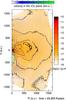 |
Fig. 6 Azimuthal average of the density and velocity fields of the collapsing core at the same time as in Fig. 5. The outflow extends up to ~1100 au. The velocities range from 0 to 4 km s-1, the density from 10-19 to 10-10 g cm-3, or from 2.4 × 10⁵ to 2.4 × 10¹³ H2 cm-3. |
4.2. Synthetic observations
We post-processed the simulation using the RADMC-3D radiative transfer code (Dullemond 2012) to compute the expected 350 GHz emission. Following Commerçon et al. (2012a,b), we assumed that the gas and dust temperature are perfectly coupled and that the dust-to-gas ratio is uniform and equal to 1%. We used the dust opacity from Semenov et al. (2003) for the homogeneous spheres model (with Fe/Fe + Mg = 0.3 “normal” silicate composition). We used the Barnard 1 distance and performed the computation for a range of inclinations i between face-on to edge-on. The emission structure is not very sensitive to the inclination between about 20° and 60°.
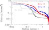 |
Fig. 7 Comparison of the radially averaged flux distribution for B1b-S (red), B1b-N (blue), and two different epochs of the MHD collapse model. The light gray curve labeled “No Disk” shows an early epoch before the formation of the FHSC, while the darker gray curve labeled “Disk” shows the later time illustrated in Figs. 5 and 6. |
4.3. Comparison of models and observations
Figure 7 presents the comparison of the radially averaged flux toward B1b-N and B1b-S with the predictions obtained from the model at two epochs. We used the views with i = 20° for two different epochs: an early stage of the collapse, 400 yr before the formation of the FHSC, when the gas structure remains close to that of an isothermal sphere and no disk is formed yet, and a late stage (6.3 × 10³ yr after the formation of the FHSC) when a rotationally supported disk has already formed, as illustrated in Figs. 5 and 6. The emission structure of the late-stage model is similar to that of the B1b protostars: both the disk radius and the predicted flux density radial distribution agree within better than a factor of two with the observations. The early-stage model presents a very different structure, with a more localized emission peak of about 0.04′′, and a rapidly decreasing flux significantly lower than that detected toward B1b-N and B1b-S, as expected from the similarity between this early stage and the simple model shown in Fig. 4. The difference of flux radial distributions between the two epochs stems from the different temperature and density distributions. In particular, the high surface brightness region is more localized when no disk is formed (0.04′′ vs. 0.2′′) because the very high density region (n(H2) > 109 cm-3) is reduced. The excellent agreement of the observed 350 GHz emission profile with the model profile confirms the high opacity of the dust emission and indicates that the dust temperature remains moderate.
To further explore the similarity of the model with the B1b-N data, we now consider the outflow spatial extend and maximum velocity, which are illustrated in Fig. 6. The values predicted by the model are fairly similar to those of B1b-N (Gerin et al. 2015). The good correspondence of the central sources’ size and shape, combined with their detection at 32 GHz, the extremely high molecular hydrogen densities and their estimated masses, support the identification of these sources with rotationally supported disks. This identification remains tentative in the absence of kinematic data, however. The sizes of the tentative disks are within a factor of a few from the predictions using the analytical expression derived by Hennebelle et al. (2016). Although fairly uncertain because we lack information about the grain emissivity law, especially when large grains are present (Dunham et al. 2014), the disk masses and temperatures are consistent with theoretical predictions of low-mass star collapse models (Masunaga & Inutsuka 2000; Machida et al. 2010; Dunham et al. 2014; Masson et al. 2016). Zhao et al. (2016) have shown that the removal of small grains can favor the formation of disks by reducing the coupling of the matter with the magnetic field, hence the efficiency of magnetic braking. The presence of large dust grains in Barnard 1b argues for a lower fraction of small dust grains in this core, which may have favored the formation of disks. We conclude that although no kinematic information is available so far, the sizes (~50 au) and brightnesses are consistent with those of rotationally supported disks formed during the collapse of dense cores in current MHD simulations. B1b-N and B1b-S thus appear to be excellent objects for testing our understanding of disk formation during low-mass protostar formation, which deserve further studies of their kinematics and spatial structure.
β is the spectral index of the dust grain emissivity at submillimeter wavelengths.
Acknowledgments
This paper makes use of the following ALMA data: ADS/JAO.ALMA#2015.1.00025.S and ADS/JAO.ALMA#2015.1.00025.S. ALMA is a partnership of ESO (representing its member states), NSF (USA) and NINS (Japan), together with NRC (Canada), NSC and ASIAA (Taiwan), and KASI (Republic of Korea), in cooperation with the Republic of Chile. The Joint ALMA Observatory is operated by ESO, AUI/NRAO and NAOJ. We acknowledge funding support from PCMI-CNRS/INSU, PNPS-CNRS/INSU, AS ALMA, Observatoire de Paris, ANR project ANR-13-BS05-0008 (IMOLABS) and the European Research Council (ERC Grant 610256: NaNOCOSMOS). We thank IRAM ARC for help with the data processing, and J. Tobin for access to the VANDAM images. We thank the referee for a careful reading of the manuscript which led to a significant improvement of our analysis. This work was performed using HPC resources from GENCI-CINES (Grant 2016-047247).
References
- André, P., Ward-Thompson, D., & Barsony, M. 1993, ApJ, 406, 122 [NASA ADS] [CrossRef] [Google Scholar]
- Chen, M. C.-Y., Di Francesco, J., Johnstone, D., et al. 2016, ApJ, 826, 95 [NASA ADS] [CrossRef] [Google Scholar]
- Ciardi, A., & Hennebelle, P. 2010, MNRAS, 409, L39 [NASA ADS] [Google Scholar]
- Commerçon, B., Launhardt, R., Dullemond, C., & Henning, T. 2012a, A&A, 545, A98 [NASA ADS] [CrossRef] [EDP Sciences] [Google Scholar]
- Commerçon, B., Levrier, F., Maury, A. J., Henning, T., & Launhardt, R. 2012b, A&A, 548, A39 [NASA ADS] [CrossRef] [EDP Sciences] [Google Scholar]
- Daniel, F., Gérin, M., Roueff, E., et al. 2013, A&A, 560, A3 [NASA ADS] [CrossRef] [EDP Sciences] [Google Scholar]
- Dullemond, C. P., Juhasz, A., Pohl, A., et al. 2012, RADMC-3D: A multi-purpose radiative transfer tool, Astrophysics Source Code Library [record ascl:1202.015] [Google Scholar]
- Dunham, M. M., Vorobyov, E. I., & Arce, H. G. 2014, MNRAS, 444, 887 [NASA ADS] [CrossRef] [Google Scholar]
- Fromang, S., Hennebelle, P., & Teyssier, R. 2006, A&A, 457, 371 [NASA ADS] [CrossRef] [EDP Sciences] [Google Scholar]
- Fuente, A., Cernicharo, J., Roueff, E., et al. 2016, A&A, 593, A94 [NASA ADS] [CrossRef] [EDP Sciences] [Google Scholar]
- Gerin, M., Pety, J., Fuente, A., et al. 2015, A&A, 577, L2 [NASA ADS] [CrossRef] [EDP Sciences] [Google Scholar]
- Harsono, D., Jørgensen, J. K., van Dishoeck, E. F., et al. 2014, A&A, 562, A77 [NASA ADS] [CrossRef] [EDP Sciences] [Google Scholar]
- Hennebelle, P., & Fromang, S. 2008, A&A, 477, 9 [NASA ADS] [CrossRef] [EDP Sciences] [Google Scholar]
- Hennebelle, P., Commerçon, B., Chabrier, G., & Marchand, P. 2016, ApJ, 830, L8 [NASA ADS] [CrossRef] [Google Scholar]
- Hirano, N., & Liu, F.-C. 2014, ApJ, 789, 50 [NASA ADS] [CrossRef] [Google Scholar]
- Hirota, T., Bushimata, T., Choi, Y. K., et al. 2008, PASJ, 60, 37 [NASA ADS] [CrossRef] [Google Scholar]
- Huang, Y.-H., & Hirano, N. 2013, ApJ, 766, 131 [NASA ADS] [CrossRef] [Google Scholar]
- I-Hsiu Li, J., Liu, H. B., Hasegawa, Y., & Hirano, N. 2017, ApJ, 840, 72 [NASA ADS] [CrossRef] [Google Scholar]
- Joos, M., Hennebelle, P., & Ciardi, A. 2012, A&A, 543, A128 [NASA ADS] [CrossRef] [EDP Sciences] [Google Scholar]
- Joos, M., Hennebelle, P., Ciardi, A., & Fromang, S. 2013, A&A, 554, A17 [NASA ADS] [CrossRef] [EDP Sciences] [Google Scholar]
- Krčo, M., & Goldsmith, P. F. 2016, ApJ, 822, 10 [NASA ADS] [CrossRef] [Google Scholar]
- Lee, K. I., Dunham, M. M., Myers, P. C., et al. 2016, ApJ, 820, L2 [NASA ADS] [CrossRef] [Google Scholar]
- Lefèvre, C., Pagani, L., Juvela, M., et al. 2014, A&A, 572, A20 [NASA ADS] [CrossRef] [EDP Sciences] [Google Scholar]
- Lis, D. C., Wootten, A., Gerin, M., & Roueff, E. 2010, ApJ, 710, L49 [NASA ADS] [CrossRef] [Google Scholar]
- Machida, M. N., Inutsuka, S.-i., & Matsumoto, T. 2010, ApJ, 724, 1006 [NASA ADS] [CrossRef] [Google Scholar]
- Masson, J., Teyssier, R., Mulet-Marquis, C., Hennebelle, P., & Chabrier, G. 2012, ApJS, 201, 24 [NASA ADS] [CrossRef] [Google Scholar]
- Masson, J., Chabrier, G., Hennebelle, P., Vaytet, N., & Commerçon, B. 2016, A&A, 587, A32 [NASA ADS] [CrossRef] [EDP Sciences] [Google Scholar]
- Masunaga, H., & Inutsuka, S.-I. 2000, ApJ, 531, 350 [NASA ADS] [CrossRef] [Google Scholar]
- Maury, A. J., André, P., Hennebelle, P., et al. 2010, A&A, 512, A40 [NASA ADS] [CrossRef] [EDP Sciences] [Google Scholar]
- Ossenkopf, V., & Henning, T. 1994, A&A, 291, 943 [NASA ADS] [Google Scholar]
- Pezzuto, S., Elia, D., Schisano, E., et al. 2012, A&A, 547, A54 [NASA ADS] [CrossRef] [EDP Sciences] [Google Scholar]
- Semenov, D., Henning, T., Helling, C., Ilgner, M., & Sedlmayr, E. 2003, A&A, 410, 611 [NASA ADS] [CrossRef] [EDP Sciences] [Google Scholar]
- Tazzari, M., Testi, L., Ercolano, B., et al. 2016, A&A, 588, A53 [NASA ADS] [CrossRef] [EDP Sciences] [Google Scholar]
- Teyssier, R. 2002, A&A, 385, 337 [NASA ADS] [CrossRef] [EDP Sciences] [Google Scholar]
- Teyssier, R., Fromang, S., & Dormy, E. 2006, J. Comput. Physics, 218, 44 [NASA ADS] [CrossRef] [Google Scholar]
- Tobin, J. J., Dunham, M. M., Looney, L. W., et al. 2015, ApJ, 798, 61 [NASA ADS] [CrossRef] [Google Scholar]
- Tobin, J. J., Looney, L. W., Li, Z.-Y., et al. 2016, ApJ, 818, 73 [NASA ADS] [CrossRef] [Google Scholar]
- Tomida, K., Okuzumi, S., & Machida, M. N. 2015, ApJ, 801, 117 [NASA ADS] [CrossRef] [Google Scholar]
- Williams, J. P., & Cieza, L. A. 2011, ARA&A, 49, 67 [NASA ADS] [CrossRef] [Google Scholar]
- Yen, H.-W., Takakuwa, S., Koch, P. M., et al. 2015, ApJ, 812, 129 [NASA ADS] [CrossRef] [Google Scholar]
- Zhao, B., Caselli, P., Li, Z.-Y., et al. 2016, MNRAS, 460, 2050 [Google Scholar]
Appendix A: Calibration
In order to check the quality of the phase-calibration transfer to the source targets for the long-baseline dataset, we first imaged the control source (J0359+3220) using the phase solution obtained on the phase calibrator (J0336+3218). However, the solution was only moderately satisfying because J0359+3220 is relatively far from the phase calibrator (5.7°), and the quasar appears slightly extended. In such conditions, the imaging results do not reflect the real performances on the targets. Therefore we performed a second test on the phase calibrator J0336+3218. In these tests, we used half of the scans observed on the phase calibrator to obtain the calibration tables, which then were used to transfer the phase calibration onto the other half of scans. For the second half, we therefore performed phase transfer instead of self-calibration. The images are acceptable for the phase-transferred scans, which shows that we can rely on the phase calibration of the targets. We also performed the cleaning in GILDAS in the same way as for the B1b sources. The resulting images are displayed in Fig. A.1.
Figure A.2 presents the amplitude versus UV distance for the combined data sets. The good overlap of the curves of flux versus UV distance in the domain from 20 m up to 600 m shows that the flux calibration is very good. B1b-N and B1b-S are heavily resolved, with most of their fluxes on short baselines.
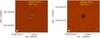 |
Fig. A.1 Point-like continuum sources J0336+3218 (left) and J0359+3220 (right) observed during the first observing session (C36-7 configuration). The yellow ellipse shows the ALMA beam. |
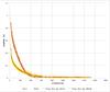 |
Fig. A.2 Amplitude of the visibility flux in Jansky versus UV distance in meters for the two data sets. The dots show the full sets of measurements, while the lines trace the moving average values using 70 points. B1b-S is shown in orange, B1b-N in yellow. |
Appendix B: Inversion of radial profile
As shown by Krčo & Goldsmith (2016), it is possible to use the radial profile of the projected 2D image of a spherically symmetrical source to retrieve the information on the initial 3D radial distribution. This appendix describes the method we applied to the submillimeter images. Assuming a spherical source of radius Rmax, at a distance D, the flux density can be expressed as the integrated emission along the line of sight: 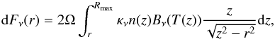 (B.1)where n is the dust density, κν is the dust emissivity, and Ω the beam size. The total flux density is then
  (B.2)Since the density and temperature only depend on the radius, it is possible to inverse the radial distribution of the flux density to derive the product of the density and Planck function n(r)Bν(T(r)). Inversion methods are rather sensitive to the noise level. We therefore chose another approach and fit the radial distributions of the flux density with an analytical radial profiles. We used the analytical solution of the inversion to determine n(r)Bν(T(r)). The two variables can be separated in a following step, using a simple assumption for the temperature profile as described in Sect. 3.2. We used a simple attenuated power-law profile for the radial distribution of the flux density (see, e.g., Krčo & Goldsmith 2016),
  (B.3)which can be easily inverted to yield
  (B.4)where Γ(x) = (x − 1) ! with x an integer number ≥2.
Developing Bν(T(r)) yields in the Rayleigh-Jeans limit  (B.5)We note that at 350 GHz, the Rayleigh-Jeans limit is only valid for T ≥ 35 K, hence it is better to use the actual Planck function. The fitting parameters for both sources are displayed in Table 2.
All Tables
All Figures
|
Fig. 1 Continuum emission at 349 GHz toward B1b-N (left) and B1b-S (right). The gray contours show the 32 GHz continuum emission from the VANDAM survey (Tobin et al. 2015, 2016) and are drawn at 0.05, 0.1, 0.2, 0.3, 0.4, and 0.5 mJy/beam. The ALMA and VLA beam sizes are shown as black and gray ellipses. The red and blue arrows show the approximate direction of the outflows. |
| In the text | |
|
Fig. 2 Fit parameters of intensity isocontours using ellipses. B1b-N data are shown in blue and B1b-S data in red. The top panel presents the variation of the major and minor axis sizes. The middle panel shows the ellipse position angle, PA, and the bottom panel the ellipticity, e = 1 − Rmin/Rmaj. The beam profiles are displayed in the top panel. The beam position angles and ellipticities are 1.1° and 0.2 for B1b-N and 16° and 0.21 for B1b-S. The upper scale displays the correspondence between antenna baseline and angular scale. |
| In the text | |
|
Fig. 3 Panel a: distribution of the circularly averaged specific intensity normalized to the peak value as a function of radius toward B1b-S and B1b-N. The gray lines show the analytical fits and the dotted lines the beam profiles. The upper scale presents the baseline in meters corresponding to the angular scale. Data for B1b-N are displayed in blue and data for B1b-S in red. Panel b: dust temperature (Td) radial distribution, assuming that the 350 GHz emission is optically thick, with a minimum value set to 12 K. Panel c: molecular hydrogen density, using the derived Td and assuming optically thin emission. This represents a lower limit to the real density. The dashed lines show the densities, assuming a constant value of the dust temperature. Panel d: cumulative mass distribution obtained by combining the information at 350 and 32 GHz. |
| In the text | |
|
Fig. 4 Top panel: variation with radius of the molecular hydrogen density, n (dash-dotted line), the column density, N (dotted line), and the resulting continuum opacity at 350 GHz, τ (solid line) for a simple spherical isothermal (12 K) core model. Bottom panel: variation of the gas mass (dash-dotted line) and 350 GHz flux (solid line) as a function of radius for the model displayed in the top panel. The dashed gray line shows the expected cumulative flux distribution for a pure blackbody (optically thick emission) at the same temperature. The observed data toward B1b-N and B1b-S are displayed in blue and red, respectively, including the ALMA data from 0.05′′ to 3′′ and JCMT and SMA data between 3′′ and 12′′ (Pezzuto et al. 2012; Hirano & Liu 2014; I-Hsiu Li et al. 2017). |
| In the text | |
|
Fig. 5 Cross section of the 3D numerical simulations showing the structure of the protostellar disk. The colors show the density field and the arrows the velocity vectors. Panel a: an edge-on view (azimuthal mean) and panel b: a face-on view of all cells that satisfy the criteria for a rotationally supported disk (Joos et al. 2012). |
| In the text | |
|
Fig. 6 Azimuthal average of the density and velocity fields of the collapsing core at the same time as in Fig. 5. The outflow extends up to ~1100 au. The velocities range from 0 to 4 km s-1, the density from 10-19 to 10-10 g cm-3, or from 2.4 × 10⁵ to 2.4 × 10¹³ H2 cm-3. |
| In the text | |
|
Fig. 7 Comparison of the radially averaged flux distribution for B1b-S (red), B1b-N (blue), and two different epochs of the MHD collapse model. The light gray curve labeled “No Disk” shows an early epoch before the formation of the FHSC, while the darker gray curve labeled “Disk” shows the later time illustrated in Figs. 5 and 6. |
| In the text | |
|
Fig. A.1 Point-like continuum sources J0336+3218 (left) and J0359+3220 (right) observed during the first observing session (C36-7 configuration). The yellow ellipse shows the ALMA beam. |
| In the text | |
|
Fig. A.2 Amplitude of the visibility flux in Jansky versus UV distance in meters for the two data sets. The dots show the full sets of measurements, while the lines trace the moving average values using 70 points. B1b-S is shown in orange, B1b-N in yellow. |
| In the text | |
Current usage metrics show cumulative count of Article Views (full-text article views including HTML views, PDF and ePub downloads, according to the available data) and Abstracts Views on Vision4Press platform.
Data correspond to usage on the plateform after 2015. The current usage metrics is available 48-96 hours after online publication and is updated daily on week days.
Initial download of the metrics may take a while.