| Issue |
A&A
Volume 602, June 2017
|
|
|---|---|---|
| Article Number | A120 | |
| Number of page(s) | 21 | |
| Section | Interstellar and circumstellar matter | |
| DOI | https://doi.org/10.1051/0004-6361/201629739 | |
| Published online | 26 June 2017 | |
Protostellar accretion traced with chemistry
High-resolution C18O and continuum observations towards deeply embedded protostars in Perseus
1 Centre for Star and Planet Formation, Niels Bohr Institute and Natural History Museum of Denmark, University of Copenhagen, Øster Voldgade 5-7, 1350 Copenhagen K, Denmark
e-mail: This email address is being protected from spambots. You need JavaScript enabled to view it.
2 Department of Physics, SUNY Fredonia, Fredonia, New York 14063, USA
3 SKA Organization, Jodrell Bank Observatory, Lower Withington, Macclesfield, Cheshire SK11 9DL, UK
4 Department of Astronomy, University of Massachusetts, Amherst, MA 01003, USA
5 Harvard-Smithsonian Center for Astrophysics, Cambridge, MA 02138, USA
6 Homer L. Dodge Department of Physics and Astronomy, University of Oklahoma, 440 W. Brooks Street, Norman, OK 73019, USA
7 Leiden Observatory, Leiden University, PO Box 9513, 2300 RA Leiden, The Netherlands
8 Department of Astrophysics, The University of Vienna, Vienna 1180, Austria
9 Research Institute of Physics, Southern Federal University, Rostov-on-Don 344090, Russia
Received: 18 September 2016
Accepted: 28 March 2017
Abstract
Context. Understanding how accretion proceeds is a key question of star formation, with important implications for both the physical and chemical evolution of young stellar objects. In particular, very little is known about the accretion variability in the earliest stages of star formation.
Aims. Our aim is to characterise protostellar accretion histories towards individual sources by utilising sublimation and freeze-out chemistry of CO.
Methods. A sample of 24 embedded protostars are observed with the Submillimeter Array (SMA) in context of the large program “Mass Assembly of Stellar Systems and their Evolution with the SMA” (MASSES). The size of the C18O-emitting region, where CO has sublimated into the gas-phase, is measured towards each source and compared to the expected size of the region given the current luminosity. The SMA observations also include 1.3 mm continuum data, which are used to investigate whether or not a link can be established between accretion bursts and massive circumstellar disks.
Results. Depending on the adopted sublimation temperature of the CO ice, between 20% and 50% of the sources in the sample show extended C18O emission indicating that the gas was warm enough in the past that CO sublimated and is currently in the process of refreezing; something which we attribute to a recent accretion burst. Given the fraction of sources with extended C18O emission, we estimate an average interval between bursts of 20 000–50 000 yr, which is consistent with previous estimates. No clear link can be established between the presence of circumstellar disks and accretion bursts, however the three closest known binaries in the sample (projected separations <20 AU) all show evidence of a past accretion burst, indicating that close binary interactions may also play a role in inducing accretion variability.
Key words: stars: formation / stars: protostars / ISM: molecules / protoplanetary disks / circumstellar matter
Current address: Institut de Ciències del Cosmos, Universitat de Barcelona, IEEC-UB, Martí Franquès 1, 08028 Barcelona, Spain.
© ESO, 2017
1. Introduction
One of the key questions of star formation regards the way in which young stellar objects (YSOs) obtain their mass. Specifically, it has not yet been established whether accretion rates onto YSOs are best characterised by a smooth decline from early to late stages or by intermittent bursts of high accretion. The question of how accretion proceeds is a central one because it holds important clues about the physical and chemical evolution of YSOs such as condensation of chondrules (Boley & Durisen 2008) and the formation of complex organic molecules (Taquet et al. 2016). While there is strong evidence of episodic accretion in the more evolved pre-main sequence stars (see Audard et al. 2014, for a recent review), it remains challenging to determine how accretion proceeds in the earliest stages of star formation. In this paper, we model the sublimation and freeze-out of CO to study the accretion histories in a sample of 24 deeply embedded protostars in the Perseus molecular cloud.
Evidence of episodic accretion in YSOs includes the FU Orionis objects (FUors), which are pre-main sequence stars showing optical luminosity bursts (Herbig 1966, 1977). Theoretically, such outbursts can be tied to accretion instabilities in the circumstellar disk encircling the YSO (e.g. Bell & Lin 1994; Armitage et al. 2001; Vorobyov & Basu 2005; Zhu et al. 2009), leading to a lot of material being dumped onto the central object over a short period of time. It is not known if deeply embedded protostars undergo episodic accretion events to the same degree as their older, more evolved counterparts, since searches for accretion bursts are most easily carried out at optical and near-infrared wavelengths where the deeply embedded objects are not detected. So far, the only direct detection of a burst in a deeply embedded object is HOPS 383, a Class 0 protostar in Orion, which increased its 24 μm flux by a factor of 35 between 2004 and 2008 (Safron et al. 2015).
Because of the challenges associated with the direct detection of episodic accretion events in deeply embedded protostars, indirect methods have been used to gather evidence of variable accretion during the embedded phase. Examples include the Class 0 protostar, L673-7, whose integrated outflow properties were used to show that its accretion rate must have been significantly higher in the past (Dunham et al. 2010). Furthermore, observations of knots in the outflows of some protostars, which can be attributed to variations in the accretion rate, can be used to estimate the interval between episodic accretion events (e.g. Bachiller et al. 1990, 1991; Lee et al. 2009; Arce et al. 2013; Plunkett et al. 2015), with studies reporting burst intervals ranging from approximately 100 yr to6000 yr.
It is also possible to use chemistry to probe the accretion histories of protostars. During an accretion burst, molecules, that are normally frozen-out onto dust grains, sublimate into the gas-phase because of the enhanced protostellar heating. Once the burst ends, the envelope cools rapidly (Johnstone et al. 2013), whereas the timescale for the molecules to refreeze back onto the dust grains is in the range 103 yr to105 yr for typical envelope densities ranging from 107 cm-3 to105 cm-3 (Rodgers & Charnley 2003). Observations of this out-of-equilibrium state, which manifests itself by stronger line intensities extending over larger areas of spatially resolved emission, may be used as a method to detect past accretion bursts (Lee 2007; Visser & Bergin 2012; Vorobyov et al. 2013; Visser et al. 2015). It is also possible to constrain the accretion history of the protostar by looking at absorption bands of interstellar ices. For example, pure CO2 ice is believed to form on dust grains during the sublimation of CO ice (Lee 2007), which indicates temperatures ≳20–30 K. Observations of pure CO2 ice absorption bands towards low-luminosity protostars have been used to show that some sources have undergone significant thermal processing in the past (e.g. Kim et al. 2012; Poteet et al. 2013).
Sample of sources.
Observing log.
One way of using chemistry to trace protostellar accretion is to measure the size of the emitting region of CO or some other molecule towards individual protostars. If the emission is detected over larger spatial scales than can be explained by the current protostellar luminosity, it will indicate that the luminosity has been larger in the past, and that the molecule is still in the process of refreezing. Such an approach was adopted by Jørgensen et al. (2015), who measured the sizes of the C18O J = 2–1 emitting regions towards a sample of 16 deeply embedded protostars and found half to show evidence of a past accretion burst. Using a large three-dimensional MHD simulation of a molecular cloud, Frimann et al. (2016) calculated synthetic C18O maps of a large sample of simulated protostellar systems and measured the sizes of the C18O-emitting regions in the same way as was done by Jørgensen et al. The study confirmed that the approach taken by Jørgensen et al. is a valid one since it demonstrated that the sizes of the C18O emission regions can be accurately measured towards systems with realistic core morphologies by an interferometer with a baseline coverage limited to ranges between 15 and 50 kλ (corresponding to angular scales between roughly 6′′ and 2′′).
 |
Fig. 1 C18O 2–1 spectra towards the peak of the integrated emission of the observed sources. The integration intervals used for producing the moment-zero maps in Fig. 2 are indicated by vertical dotted lines and run from −2.5σ to 2.5σ of the fitted Gaussians (black dashed lines). The numeric value in the top left corner of each panel is the integrated emission over the line. |
This paper presents continuum and C18O 2–1 observations towards a sample of 24 embedded protostars in the Perseus molecular cloud (distance: 235 pc; Hirota et al. 2008). The aim of the paper is to measure the sizes of the C18O-emitting regions towards the observed protostars and to use those measurements as a tracer of past accretion bursts. Furthermore, the continuum observations are used to investigate whether or not a link between accretion bursts and circumstellar disks can be established. The key advantages of this sample, relative to the one analysed in Jørgensen et al. (2015), are that all the protostars are from the same molecular cloud, meaning that distance uncertainties do not play a role, and that the star formation environments are similar. Also, the observations are all from the same program, which provides a more uniform sample. The observations are from the large survey “Mass Assembly of Stellar Systems and their Evolution with the SMA” (MASSES; Co-PIs: Michael M. Dunham and Ian W. Stephens) undertaken with the Submillimeter Array (SMA). The survey targets all known embedded protostars in Perseus, including the 66 sources identified with the Spitzer Space Telescope by Enoch et al. (2009) and seven candidate first hydrostatic cores. The survey is still ongoing, hence this paper comprises the sample of sources imaged thus far. The first results from MASSES were presented by Lee et al. (2015, 2016).
The paper is laid out as follows: Sect. 2 describes the observations and introduces the observed sample. Section 3 describes the procedure used for measuring the sizes of the C18O-emitting regions, while Sect. 4 presents the results of the analysis of both the C18O and continuum data. Depending on the adopted CO sublimation temperature, between 20% and 50% of the observed sources show evidence of a past accretion burst, which is consistent with the results of Jørgensen et al. (2015). Section 5 presents a discussion of the results including possible links between episodic accretion and circumstellar disks and between episodic accretion and multiple systems. Finally, Sect. 6 summarises the findings of the paper.
2. Observations
2.1. SMA
The observations were carried out with the SMA (Ho et al. 2004), a submillimetre and millimetre interferometer, consisting of eight 6 m antennae situated on the summit of Mauna Kea, Hawaii. The data include observations of the C18O 2–1 transition (rest frequency: 219.56 GHz) and 230 GHz (1.3 mm) dust continuum observations. All of the data were taken in the array’s subcompact configuration, which typically covers baselines between 5 kλ and 50 kλ. For some targets, C18O observations from the extended configuration are also available (typical baseline coverage between 20 kλ and 150 kλ), which are concatenated with the subcompact data whenever available. The data were reduced and calibrated with the MIR package1 using standard calibration procedures, while imaging was done using Miriad (Sault et al. 1995). Table 1 lists the objects in the observed sample along with their Spitzer positions, luminosities, and bolometric temperatures, while Table 2 presents a log of the observations. For further details on the data reduction process, the reader is referred to Lee et al. (2015).
 |
Fig. 2 Maps of C18O 2–1 integrated emission (line contours) and 1.3 mm continuum emission (colour map). Contours are drawn starting from 3σ in steps of 6σ (see Table 2 for C18O and continuum 1σ rms sensitivities). Synthesised beams of the C18O and continuum emission are shown in the lower left corners as respectively black and a shaded ellipses. Note that the beam sizes only differ significantly for the targets where extended data is available for the C18O emission. The blue symbols mark the source positions from the VANDAM survey (Tobin et al. 2016), with crosses indicating single protostars and triangles indicating multiple systems with projected separations <0.8′′. |
Figure 1 shows C18O 2–1 spectra extracted towards the peak of the integrated emission of each source. The area between the dotted lines indicates the integration intervals used to produce the C18O moment-zero maps shown in Fig. 2. The intervals are determined by Gaussian fits and run between −2.5σ and 2.5σ. As seen from the spectra, essentially all of the emission is recovered towards the individual sources. Only Per-emb 27 has its upper integration limit increased by 0.5 km s-1 to catch additional red-shifted emission. Figure 2 also shows continuum maps of the observed sources. The emission is observed to be relatively compact towards the individual sources, with some evidence of low surface brightness extended emission toward some sources.
The blue symbols in Fig. 2 indicate source positions from the “VLA Nascent Disk and Multiplicity Survey of Perseus Protostars” (VANDAM) survey (Tobin et al. 2016). Crosses are used for single protostars, while triangles indicate multiple systems with projected separations <0.8′′. The triangles all represent binary systems except for Per-emb 33, which is a triple system. Of the 24 sources in the sample, ten are part of multiple systems not resolved in the SMA maps. The sources are labelled according to the naming scheme of Enoch et al. (2009), who used Spitzer observations to identify the protostars. The size of the Spitzer beam at 24 μm is 7′′, meaning that if a multiple system is not resolved in the SMA observations it will not have been resolved in the Spitzer 24 μm observations either, and the label covers all members of the system.
 |
Fig. 3 Examples of posterior parameter distributions of three fitted parameters towards Per-emb 1. The green lines represent the medians of the distributions and the shaded areas the 1σ uncertainty region. The median value and uncertainty are printed in the upper right corner of each panel. |
The addition of extended SMA data does not alter the C18O maps. This is related to the fact that C18O is typically not detected at baselines ≳50 kλ. The addition of extended data is still advantageous, as it provides additional baselines down to ≈20 kλ, thereby improving the signal at intermediate baselines. As a test of consistency between the samples, the C18O 2–1 observations of the nine Perseus protostars from the Jørgensen et al. (2015) survey are also included. Only one of these nine sources, IRAS 03256, is not part of the sample analysed here. Going forward, the two samples are distinguished by referring to the “MASSES” sample and the “JVWB15” sample, respectively.
2.2. JCMT/SCUBA
The large-scale emission of the observed sources is traced with 850 μm single-dish continuum observations from the James Clerk Maxwell Telescope Submillimetre-Common Bolometer Array (JCMT/SCUBA) legacy catalogue (Di Francesco et al. 2008). The SCUBA maps have a resolution of 15′′, and all the sources in the sample are detected except for Per-emb 47.
3. Model fitting
To measure the sizes of the C18O-emitting regions towards the observed sources, we follow the approach of Jørgensen et al. (2015) and Frimann et al. (2016) and fit Gaussians to the interferometric data directly in the (u,v)-plane, thereby avoiding uncertainties introduced by the deconvolution procedure. Miriad’s uvfit routine can be used to fit the Gaussians, but we find that its results can be sensitive to the starting guess of the fitting parameters, which indicates that it does not always converge to the optimal result. To circumvent this issue, the Gaussians are instead fitted using the Python Markov chain Monte Carlo (MCMC) code emcee2 (Foreman-Mackey et al. 2013). An MCMC method has the advantage that it is capable of exploring the parameter space better relative to a standard non-linear fitting algorithm, like the one used by uvfit.
Any MCMC algorithm needs a likelihood function describing the probability of the data given a set of input parameters, as well as prior probabilities of the parameters. The likelihood function used here takes the form ![Mathematical equation: \begin{eqnarray*} \mathcal{L}\left(\vec{p}\right) = \left(\sum_{i=1}^N \left[d_i - m_i\left(\vec{p}\right)\right]^2\right)^{-\frac{N}{2}}, \nonumber \end{eqnarray*}](/articles/aa/full_html/2017/06/aa29739-16/aa29739-16-eq21.png) where the sum is over the individual data points, di, and m(p) is the model function with fitting parameters p. This likelihood function is appropriate for situations where one is ignorant of the uncertainties on the individual data points (e.g. Chap. 9 of Gregory 2005). The model function, m, is a two-dimensional Gaussian function described by six parameters: the total flux; the peak position relative to the phase-centre in the RA (Right ascension) and Dec (declination) directions; the average full width at half maximum (FWHM) of the Gaussian,
where the sum is over the individual data points, di, and m(p) is the model function with fitting parameters p. This likelihood function is appropriate for situations where one is ignorant of the uncertainties on the individual data points (e.g. Chap. 9 of Gregory 2005). The model function, m, is a two-dimensional Gaussian function described by six parameters: the total flux; the peak position relative to the phase-centre in the RA (Right ascension) and Dec (declination) directions; the average full width at half maximum (FWHM) of the Gaussian,  , where FWHMmin and FWHMmaj are the minor and major axes; the ratio between the major and minor axes, FWHMmaj/FWHMmin; and the position angle of the Gaussian. We are largely ignorant of the prior probabilities and therefore set them as widely as possible. For the total flux, FWHMavg, and FWHMmaj/FWHMmin, the prior probabilities are assumed to be flat in log-space between 0.1 Jy.km.s-1 and 100 Jy.km.s-1, 0.1′′ and 100′′, and 1 and 100. For the peak position, the prior probability is assumed to be flat within a radius of 5′′ from the peak position estimated from the moment-zero maps. Finally, the prior probability of the position angle is assumed to be flat between 0◦ and 180◦. We note that as long as the priors are set wide enough, they do not influence the fitting results.
The result of the MCMC fitting is the posterior probability distribution, which can be marginalised and drawn as one-dimensional distributions for each parameter (see Fig. 3 for examples). The distributions are typically, but not always, well represented by Gaussians, and the results are therefore reported by giving the distribution’s median with the 16th and 84th percentiles approximating the lower and upper bound of the uncertainty. The sources are also fitted using Miriad’s uvfit routine. The results of the two methods deviate significantly for five out of 24 sources. For those sources where the two methods do not agree, we confirm that emcee converges to a result with a lower sum of the squared residuals than uvfit.
 |
Fig. 4 (u,v)-amplitude plots of the integrated C18O emission towards the sources in the observed sample. The grey dotted histograms in each panel indicate the expected amplitude in the absence of any source emission. The solid green line in each panel represents the best fitting Gaussian, while the shaded region indicates the 1σ uncertainty region of the fit. The vertical axis of each panel has been scaled to the Gaussian’s peak flux, whose value is printed in the upper right. The grey dashed lines indicate the 15 kλ lower boundary of the fit. Panels where the (u,v)-amplitudes have been plotted in grey indicate objects whose fits have been rejected (see text for details). |
4. Results
4.1. C18O observations
Using the method described in Sect. 3, two-dimensional Gaussians are fitted to the integrated C18O visibilities of all 24 sources in the sample. The smallest baselines, which correspond to large-scale emission, are excluded as they may include emission that is not regulated by the protostellar heating. Emission from extended spatial scales may instead be the result of heating by the interstellar radiation field, or it may originate from low-density pre-depletion regions where CO has not yet frozen out (Jørgensen et al. 2005b). Here, we follow Jørgensen et al. (2015) and only include baselines above 15 kλ, corresponding to angular scales ≲6′′.
Gaussian fitting results towards the integrated C18O emission.
Figure 4 shows (u,v)-amplitudes and Gaussian fits of the observed sources. The (u,v)-amplitudes implicitly assume axial symmetry around the centre so, for those fields that contain multiple emission peaks, the emission that does not pertain to the source of interest is subtracted out before plotting the (u,v)-amplitudes. The subtraction is done by fitting a Gaussian to the secondary emission in the moment-zero map and then subtracting that Gaussian directly from the interferometric visibilities; if necessary this procedure may be repeated several times. The subtraction is solely for the benefit of being able to display the (u,v)-amplitudes of sources located in fields with multiple emission peaks. For the actual model fitting, the original non-subtracted data are always used, and multiple Gaussians are fitted to fields with more than one emission peak.
Table 3 shows the results of the Gaussian fits to the sources in the MASSES sample. For most of the sources, the statistical uncertainties of the measured values of FWHMavg (hereafter referred to as the measured extents) are less than 0.5′′. Also, the fitted Gaussians are relatively circular, with most fits having FWHMmajor/FWHMminor≤ 1.5 (see Sect. 5.2 for a discussion of the causes of asymmetric emission).
Per-emb 25, 28, 47, and 61 are excluded from further analysis, as their signal-to-noise ratios are too small to measure the extents reliably. The low signal-to-noise ratios may themselves be an indirect clue that the four sources have not recently undergone an accretion burst, since the elevation of CO ice into the gas phase is expected to enhance the strength of the emission (Visser et al. 2015; also see discussion in Sect. 5.1). Three of the sources have a measured Lbol < 1 L⊙, and it is therefore not surprising that their emission is too weak to be measured reliably. The low signal-to-noise ratios may also indicate that the sources are surrounded by small amounts of envelope material. This scenario seems particularly likely for Per-emb 47, which is not detected in the SCUBA maps, but is also likely for both Per-emb 25 and 63, both of which have small inferred envelope masses (cf. Sect. 4.2). Naturally, the two scenarios are not mutually exclusive. Per-emb 42 is excluded from the subsequent analysis, not because of a lack of signal, but because its emission cannot be properly untangled from the emission of the nearby 9.2 L⊙ protostar Per-emb 26.
 |
Fig. 5 Measured C18O extents versus the current (bolometric) luminosity. Triangular symbols represent sources that are associated with a companion protostar at a projected distance <0.8′′. The error-bars indicate the statistical uncertainties of the measurements listed in Table 3. The uncertainties of the luminosities are not shown to avoid cluttering the diagram, but they are small enough that they do not influence the conclusions. The solid line represents the expected CO extent given the current luminosity and a CO sublimation temperature of 28 K, while the dashed lines represent the expected CO extents for 10 and 100 times the current luminosity. The dash-dot line shows the expected CO extent for a sublimation temperature of 21 K. The horizontal dotted line at 1.4′′ indicates the lower limit of the extents that can be measured given the baseline coverage and sensitivity of the observations. |
Figure 5 shows the measured C18O extents versus the current (bolometric) luminosity, Lcur, of the protostars in the MASSES sample. In the absence of any past accretion variability and for an adopted CO sublimation temperature of 28 K, the measurements are expected to follow the blue line, which has been calculated from synthetic observables of a set of axissymmetric radiative transfer models, presented in Appendix B. The line is described by the equation  (1)where d is the distance to the source, and the angular coefficient, a, depends on the adopted sublimation temperature. For Tsub = 28 K, appropriate for CO ice mixed with water (Noble et al. 2012), a = 0.89″. For Tsub = 21 K, appropriate for pure CO ice (Sandford & Allamandola 1993; Bisschop et al. 2006), a = 1.64″.
Many of the sources shown in Fig. 5 have measured extents that are larger than predicted, particularly for the sources with Lbol ≲ 2 L⊙. It is natural to suspect that this could be an indication of an instrumental bias of the interferometer. We will argue in Sect. 5.1 that this is not the case, and that the measured extents are reliable. However, at the same time it is also likely that the four sources that were excluded due to overly small signal-to-noise ratios have small C18O-emitting regions that could not be accurately measured due to a combination of sensitivity and baseline issues.
Choosing a lower baseline limit of 15 kλ has the effect of excluding all emission on angular scales ≳6′′. Such a limit clearly inhibits the measurement of intense bursts that elevate CO into the gas phase over large regions, but it is necessary to avoid contamination from regions where the C18O emission is not regulated by the heating from the central protostar. Based on measurements of synthetic data, Frimann et al. (2016) found that it is typically safe to include baselines down to 10 kλ (angular scale of 9′′), before one begins to run into issues with large-scale emission not associated with the heating from the central source. However, it should be noted that the synthetic data did not include sources with multiple emission peaks, which means that the large-scale emission was less confused than is often the case here. Redoing the analysis with a lower boundary of 10 kλ alters the results substantially (by more than 1σ in the fitting uncertainty) for only three objects, Per-emb 2, 16, and 18, that are listed in the bottom of Table 3. For Per-emb 2, it is difficult to judge which of the two measurements is most accurate, but both yield a measured extent that is significantly enhanced relative to what is expected from the current luminosity. Since the difference is not crucial to the conclusions, we retain the lower boundary of 15 kλ, which gives the most conservative estimate of the burst magnitude. For Per-emb 16, the measured extent, given a baseline limit of 10 kλ, is significantly larger than the apparent extent of the source in the moment-zero map, and we therefore retain the 15 kλ limit. For Per-emb 18, it can be seen in the moment-zero map that the C18O emission towards the source is indeed very extended, and the 10 kλ measurement is adopted going forward.
By solving Eq. (1)for the luminosity, it is possible to calculate the luminosity, LCO, needed to produce the measured size of the C18O-emitting region. If accretion has been steady for longer than one freeze-out time, LCO should not be very different from the measured luminosity; on the other hand, if the source has recently undergone an accretion burst, LCO will be enhanced relative to the measured luminosity. The ratio, LCO/Lcur, can therefore be used to determine if a source has undergone an accretion burst in the past, and to estimate the magnitude of the burst. The calculated LCO/Lcur ratios are listed in Table 3 for adopted sublimation temperatures of both 21 K and 28 K.
Continuum fluxes and inferred masses.
4.2. Continuum observations
Given the resolution of the data, it is not possible to unambiguously detect circumstellar disks. Instead, continuum observations can be used to measure excess compact emission towards the individual sources, which might then indicate the presence of a disk (Looney et al. 2000; Harvey et al. 2003; Jørgensen et al. 2005a, 2009; Enoch et al. 2011). Here, we use the SMA continuum observations to calculate the compact masses towards the sources in the sample. Single-dish JCMT continuum observations from the SCUBA Legacy Catalogue (Di Francesco et al. 2008) are used to calculate the envelope masses and to correct the compact masses for contamination from the envelope.
The compact fluxes are measured by fitting unresolved point sources to the 1.3 mm SMA continuum data at baselines >40 kλ using Miriad’s uvfit routine. At such long wavelengths, the dust emission can be assumed to be optically thin meaning that, for a constant temperature, the dust emission will be proportional to the dust mass. To calculate the total dust plus gas mass of the compact emission, we use the formula  where Fν is the measured flux density of the source; ℛgd is the gas-to-dust mass ratio, assumed to be 100; d is the distance to the source; Tdust is the dust temperature, assumed to be 30 K (Dunham et al. 2014); and the dust opacity, κν, is taken to be 0.899 cm2 g-1 (Ossenkopf & Henning 1994; coagulated dust grains with thin ice-mantles at a density of nH2 ~ 106 cm-3, commonly referred to as OH5). Such a mass estimate is associated with a number of uncertainties arising from the assumed gas-to-dust mass ratio, the distance uncertainty, the adopted dust opacity, the assumed dust temperatures, and the degree of contamination from the large-scale envelope on the compact emission, amounting to a total uncertainty approaching an order of magnitude (Dunham et al. 2014).
The sources are embedded within massive envelopes that can be traced with single-dish continuum observations. As with the compact emission, the large-scale emission can be converted into a mass estimate of the envelope. However, on such large scales the physical structure of the envelope, as well as the heating from the central protostar, must be taken into account. Based on radiative transfer models with power law envelopes, ρ ∝ r-1.5, Jørgensen et al. (2009) derived an empirical relationship between the source flux and the envelope mass  which is adopted to calculate the envelope mass. Like the compact mass, this quantity is associated with order of magnitude uncertainties arising from the gas-to-dust ratio, the adopted dust opacity, and the assumed envelope structure.
 |
Fig. 6 Histograms of compact masses inferred from continuum flux densities at baselines >40 kλ. The black histograms show the full sample while the shaded histograms show only the sources that are identified as disk candidates in Table 4. The top panel shows uncorrected compact masses, while the bottom panel shows compact masses corrected for the envelope contribution using the method of Jørgensen et al. (2009). |
The emission from the large-scale envelope is mostly resolved out at baselines >40 kλ, however, depending on the strength of the compact emission, the envelope flux may still contribute significantly (e.g. Dunham et al. 2014). Jørgensen et al. (2009) calculated that, for a power law envelope with ρ ∝ r-1.5, approximately 4% of the 850 μm single-dish flux leaks into the interferometric flux, measured at 1.1 mm, and they therefore subtracted that fraction from their interferometric fluxes. The same method is employed here, except that only 2% of the single-dish flux is subtracted, to reflect the fact that the interferometric observations in this study are taken at a wavelength of 1.3 mm instead of 1.1 mm.
Fluxes and inferred masses are listed in Table 4 along with a column showing whether or not a given source has been identified as a disk candidate in high-resolution continuum observations. The corrected compact measurements of Per-emb 16 and 28 are negative, meaning that the contamination from the shared envelope between the two sources has been over estimated, which indicates that the real envelope emission is less centrally condensed than assumed (i.e. has a shallower power law slope than 1.5). Figure 6 shows the distribution of compact masses. The medians of the corrected and non-corrected mass distributions are 0.06 M⊙ and 0.08 M⊙ respectively, and there is no significant difference between the median mass of the full sample and that of the disk candidates. The widths of both distributions span more than an order of magnitude, in agreement with the results of other continuum surveys (Jørgensen et al. 2009; Enoch et al. 2011; Tobin et al. 2015b), and there is no discernible difference between the distributions covering the full sample and the one covering only the disk candidates (a Kolmogorov-Smirnov test yields a p-value of 0.55, meaning that the null hypothesis that the two samples are drawn from the same distribution cannot be rejected). This finding indicates that one should be careful about interpreting a high compact mass as evidence of a circumstellar disk, although we cannot rule out that the compact masses are correlated with the disk masses.
5. Discussion
5.1. Reliability of measured extents
Given the limited baseline coverage and sensitivity of the observations there is also a limitation on how small C18O extents can be measured from the observations. This issue is addressed in Appendix B where we find that it should be possible to measure the size of the C18O-emitting region down to angular scales of ≈1.4′′. In this section we discuss the reliability of the measured extents by comparing the measurements directly to theoretical (u,v)-amplitudes as well as to results from other observational studies.
 |
Fig. 7 Comparison between observed and calculated (u,v)-amplitudes towards Per-emb 2 and 19. The calculated (u,v)-amplitudes are obtained from the axissymmetric models presented in Appendix B. In both cases we adopt an envelope power-law index of 1.5 and outflow half opening angle of 10◦. The adopted disk and envelope masses are printed in the panels and were motivated by the measured masses listed in Table 4. The model visibilities are averaged over 11 viewing angles and are shown as solid lines with shaded 1σ uncertainty regions. To account for the degeneracy between the assumed model masses and CO abundances, the model visibilities are normalised to the integrated single-dish flux density of each of the sources. The flux densities were estimated by convolving the moment-zero maps with a 20′′ Gaussian beam before reading the flux density at the source position. The red and blue model visibilities show the expected (u,v)-amplitudes for the current luminosity and for the luminosity needed to provide a good fit to the measured data. Panels to the left adopt a sublimation temperature of 28 K while panels to the right assume a sublimation temperature of 21 K. |
Figure 7 compares the measured (u,v)-amplitudes towards Per-emb 2 and 19 to the calculated (u,v)-amplitudes based on the axissymmetric radiative transfer models presented in Appendix B. These two sources were chosen because both have a low current luminosity (0.9 L⊙ and 0.4 L⊙ respectively) and because both show evidence of a past accretion burst. Calculating the (u,v)-amplitudes for a model based on the measured bolometric luminosities of the sources yields a poor fit to the data regardless of whether one adopts a CO sublimation temperature of 28 K or 21 K (red lines in Fig. 7). To provide a good fit to the data, the protostellar luminosity of the model has to be increased by the factor indicated by the LCO/Lcur ratios listed in Table 3 (blue lines in Fig. 7). Based on the comparison between the calculated and observed (u,v)-amplitudes we conclude that the large sizes of the C18O-emitting regions measured towards many of the low-luminosity sources in the sample are real and not a measurement bias of the interferometer.
For bolometric luminosities ≤3 L⊙ the predicted size of the C18O-emitting region is smaller than its smallest measurable size, which may explain why all of the low-luminosity sources lie well above the solid blue line in Fig. 5. In Sect. 4.1, four sources, all with Lbol ≲ 1.2 L⊙, were excluded from the sample because the sensitivity of the observations was not high enough to measure the extents reliably. Since the elevation of CO into the gas-phase over a large region is itself expected to increase the strength of the emission, which in turn will make the extent easier to measure, it seems likely that the four excluded sources have not recently undergone an accretion burst and we therefore count them to the “no-burst” group when addressing the burst statistics in Sect. 5.3.
To test whether the results are consistent over different data sets, the MASSES and JVWB15 measurements are compared to one another. The original JVWB15 extents reported by Jørgensen et al. (2015) were measured using Miriad’s uvfit routine. To make a direct comparison possible, the JVWB15 data have been reanalysed using the procedure described in Sect. 3. A description of the reanalysis along with a comparison to the original results is presented in Appendix A. The rightmost column of Table 3 lists the (re)-measured extents of the JVWB15 sources. The only source whose measured extent is not consistent with its MASSES counterpart within 2σ is Per-emb 13, which has a measured extent of 3.9′′ in the MASSES sample and 0.5′′ in the JVWB15 sample. A closer examination of the fitting results and (u,v)-amplitudes (see Fig. A.1) reveals that the JVWB15 emission is consistent with a point source, and that all extents ≲2′′ fit the data well. While closer, it is still significantly less than the measured extent of the MASSES source.
The sizes of the C18O-emitting regions towards Per-emb 12, 13, and 26 have also recently been measured by Anderl et al. (2016) using sub-arcsecond observations taken with the IRAM Plateau de Bure Interferometer. Their measurements, obtained by fitting two-dimensional Gaussians to maps of integrated emission, are in excellent agreement with our own and are given as: (5.4 ± 0.1) arcsec for Per-emb 12; (3.3 ± 0.1) arcsec for Per-emb 13; and (3.5 ± 0.2) arcsec for Per-emb 26.
5.2. Emission asymmetry
On average, the ratio between the major and minor axes of the Gaussian fits listed in Table 3 is 1.5 with individual values ranging from 1.06 to 2.5 (accepted fits only). The emission may appear elongated for several reasons; the gas and dust surrounding the individual sources likely deviate from spherical symmetry, which can influence the morphology of the emission; some sources (e.g. Per-emb 35 and 44) contain several protostars that are close enough together that they are not resolved by the interferometer, but far enough apart that the shape of the emission is affected; finally, the emission may be elongated in the direction of the outflow. In the first two cases it is appropriate to use the method applied in this study and calculate an average size of the C18O-emitting region from the minor and major axes of the fitted Gaussian. However, if the emission is elongated along the outflow axis, it may be more appropriate to take the FWHM in the direction perpendicular to the outflow axis because the temperatures in the outflow cone are significantly enhanced and CO therefore sublimates at larger radii.
 |
Fig. 8 Top: cumulative distribution function of the difference between the Gaussian and outflow position angles. The dotted line shows a uniform distribution expected for a random relative orientation. Bottom: FWHMmajor/FWHMminor versus relative position angle. |
Outflow and Gaussian position angles.
We investigate whether or not the position angles of the fitted Gaussians tend to be aligned with the outflow axes. Table 5 lists outflow and Gaussian position angles for all sources in the sample where the Gaussian fit was accepted and where we could find a measurement of the outflow position angle in the literature. The top panel of Fig. 8 shows the cumulative distribution of the relative position angles between Gaussians and outflows (solid line) along with the uniform cumulative distribution (dotted line). Performing a Kolmogorov-Smirnov test on the distribution with null hypothesis that the observed and random distributions are the same yields a p-value of 0.46. Adopting the canonical significance threshold of 0.05, the null hypothesis can therefore not be rejected, and the measurements are consistent with being drawn from a distribution with no preferred alignment. In the bottom panel of Fig. 8 we plot the ratio between the Gaussian major and minor axes against the relative position angle. The aim of this is to investigate whether or not more elongated emission has a stronger tendency towards alignment with the outflow axis. The figure reveals no such correlation and we therefore conclude that there is no general tendency towards alignment between the outflow axes and the Gaussian major axes.
While we reject a general connection between elongated emission and outflow axes, there are a few individual sources where it appears likely that the elongation is caused by the outflow. This is the case for Per-emb 1, 13, and 27, all of which are known to drive strong outflows and all of which have relative position angles ≤10◦. Among the three sources FWHMavg and FWHMminor differ by 34% in the most extreme case. Changing the reported extent from FWHMavg to FWHMminor may thus affect the conclusions for the individual sources but will not affect the conclusions of the sample as a whole.
Frimann et al. (2016) studied synthetic C18O maps towards a sample of 2000 embedded protostars in a large three-dimensional MHD simulation of a molecular cloud, and fitted Gaussians to their synthetic data in the same manner as is done in this study. On average, they found a ratio between the major and minor axes of the fitted Gaussians of 1.2; somewhat below the average value of 1.5 found in this study. However, the authors did not add noise to their synthetic observables nor did they adopt a realistic sampling of the (u,v)-plane, which may explain the difference. We have therefore taken the synthetic data from the numerical study and applied noise and (u,v)-sampling similar to what is available in the observations (see Sect. B.3 for details). Calculating the average ratio between the Gaussian major and minor axes of the new data gives a value of 1.6, which is similar to the 1.5 measured here. It is worth noting that while the resolution of the MHD simulation studied by Frimann et al. (2016) was large enough to resolve the protostellar cores, it was not large enough to resolve the launching region of protostellar outflows. The study also did not include any multiple systems, which means that the elongation measured in the Gaussian fits must be due to deviations from spherical symmetry of the material surrounding the protostars, as well as overall uncertainties introduced when adding noise and a realistic (u,v)-sampling to the synthetic observations.
5.3. LCO/Lcur as a tracer of past accretion bursts
The main tracer used for detecting past accretion bursts is the ratio, LCO/Lcur, the calculation of which is associated with a number of uncertainties. These arise from statistical and systematic measurement uncertainties of the C18O extents and bolometric luminosities, as well as from uncertainties and assumptions pertaining to the models that went into calculating Eq. (1). While statistical uncertainties are accounted for when calculating LCO/Lcur, systematic and model uncertainties are not. Some of these uncertainties are discussed in Appendix B, which presents the radiative transfer models that were used to derive Eq. (1). The appendix examines how the physical structure of the disk, envelope, and outflow affects the measured luminosities and C18O extents. Other uncertainties, such as Lbol uncertainties originating from incomplete sampling of the SED or calibration uncertainties of the observations, are more difficult to track, but the fact that the studied sample consists of more than 20 sources helps even those out.
A key assumption concerning Eq. (1)regards the temperature at which CO ice sublimates from the dust grains. In the calculation leading up to Eq. (1)two sublimation temperatures were considered: Tsub = 28 K appropriate for CO ice mixed with water (Noble et al. 2012), and Tsub = 21 K appropriate for pure CO ice (Sandford & Allamandola 1993; Bisschop et al. 2006). A low sublimation temperature would explain the extended C18O emission measured towards some sources, but it struggles to explain the compact emission observed towards others (cf. Fig. 5). Observationally, there is some evidence that the sublimation temperature of CO in cores is higher than the 21 K expected for pure CO ice, with studies reporting values in the range 24–40 K (Jørgensen et al. 2005b; Yıldız et al. 2012, 2013; Anderl et al. 2016). Studies of disks have found even lower CO sublimation temperatures of 17–19 K (Qi et al. 2013; Mathews et al. 2013). However, the different sublimation temperatures inferred for the disks may be explained by thermal processing of the disk material, which can create an “onion shell” structure of the ices on the dust grains with separated layers of pure ices (Jørgensen et al. 2015).
In general, one can consider the evidence of a past accretion burst to grow stronger as the ratio LCO/Lcur increases. If we follow Jørgensen et al. (2015) and only consider sources with  , 12 out of 23 sources (52%) show evidence of a past accretion burst. This statistic excludes Per-emb 42, whose emission could not be disentangled from that of Per-emb 26, but includes Per-emb 25, 28, 47, and 61 which we consider no-burst sources (cf. Sect. 5.1). Considering
  the statistics change so that 4 out of 23 sources (Per-emb 2, 11, 16, and 19; 17%) continue to show evidence of a past accretion burst. In either case, a significant fraction of the sources show evidence of having undergone an accretion burst in the not so distance past. We note that even though the LCO/Lcur ratio gives an indication of the burst magnitude, it is not constant with time but will start decreasing as CO begins to refreeze. Also, the exclusion of baselines below 15 kλ means that we are unable to measure large extents, which may lower the measured LCO/Lcur ratios towards some of the high-luminosity sources. Because of these uncertainties, we consider all sources with LCO/Lcur> 5 to show evidence of a past accretion burst even though classical FUor accretion bursts show luminosity enhancements of an order of magnitude or greater.
5.4. Burst intervals
The time it takes for the molecules to freeze back onto the dust grains following a burst is inversely proportional to the density (Rodgers & Charnley 2003). The length of the time interval where it is still possible to observe the spatially extended C18O emission therefore depends both on the magnitude of the burst (high-intensity bursts push the CO ice-line out to larger radii where the freeze-out timescale is longer) and on the physical structure of the envelope. Knowledge of the freeze-out timescale, tdep, can be used to estimate the time interval between bursts, Tburst. Assuming that the duration of the burst itself is negligible, the average interval between bursts can be estimated by noting that the ratio tdep/Tburst should be equal to the fraction of sources that show evidence of having undergone an accretion burst in the past. For a sublimation temperature of 28 K this suggests Tburst ≈ 2 × tdep and for a sublimation temperature of 21 K it suggests Tburst ≈ 5 × tdep. For an average freeze-out timescale of 10 000 yr, appropriate for an envelope density of 106 cm-3 (Rodgers & Charnley 2003; Visser & Bergin 2012), a rough estimate of the burst interval is thus 20 000–50 000 yr.
Scholz et al. (2013) used a direct observational approach to estimate the average burst interval of YSOs. Utilising mid-infrared photometry from Spitzer and the Wide-field Infrared Survey Explorer (WISE), they identified five burst candidates in a sample of 4000 YSOs observed over two epochs set five years apart. Based on their analysis, Scholz et al. (2013) argued for an average burst interval in the range 5000 yr to50 000 yr. A different approach was adopted by Offner & McKee (2011) who used the local star formation rate and number of identified FUors to infer that YSOs spend ~1200 yr undergoing accretion bursts. Assuming a 100 yr burst life-time and an average protostellar lifetime of 0.5 Myr, the time between bursts is ~40 000 yr. Both these observational estimates are in good agreement with the rough estimate from above. Estimates of burst intervals can also be gained from numerical simulations. Using hydrodynamical simulations, Vorobyov & Basu (2015) found that episodic accretion events induced by gravitational instabilities and disk fragmentation are present during the early evolution of most protostellar systems. The average burst interval ranges from 0.3 × 10⁴ yr to1.1 × 104 yr depending on the initial conditions of the model; somewhat below but at the same scale as the estimate above.
To accurately estimate the average burst interval, observations over long time baselines and/or large sample sizes are needed. For example, for an assumed average burst interval of 20 000 yr and a sample size consisting of 4000 sources, a time baseline ≳30 yr is needed to constrain the length of the burst interval to a factor of two or better. Similarly, for a time baseline of 5 yr a sample size ≳20 000 is needed to constrain the length of the burst interval (Hillenbrand & Findeisen 2015). Such large surveys are challenging to perform, particularly for deeply embedded Class 0 and I protostars that are only detected at far-infrared wavelengths and beyond. One of the advantages of using freeze-out and sublimation chemistry to trace past accretion bursts is that the effective time baseline for the observations is equal to the freeze-out time of the molecules. With freeze-out times generally expected to exceed 103 yr, it should therefore be possible to constrain the burst interval to within a factor of two, with a sample comprised of tens of objects instead of thousands of objects. To actually do this requires careful modelling of the envelope structure to better constrain the freeze-out timescale, as well as observations of a molecule other than CO, with another freeze-out timescale, to further decrease uncertainties. A good candidate molecule for follow-up observations is formaldehyde (H2CO), which has a sublimation temperature, Tsub = 38 K (Aikawa et al. 1997), that is low enough that the extent of its emission should still be measurable with an interferometer such as the SMA.
5.5. Link to circumstellar disks
Given that episodic outbursts are thought to arise from instabilities in circumstellar disks, it is of particular interest to investigate whether or not evidence of a past accretion burst can be linked to the presence of a circumstellar disk. The majority of the sources in the observed sample drive outflows, which already indicate that they are encircled by a disk, but not necessarily a large or massive one. A classical FUor accretion burst, with an accretion rate of 10-4 M⊙ yr-1 lasting 200 yr, will accrete 0.02 M⊙ onto the protostar, indicating that the disk has to be fairly massive to sustain such a burst. Furthermore, for gravitational instabilities to operate, disk masses ≳0.05 M⊙ are needed (Vorobyov 2013; Kratter & Lodato 2016). Although magnetic and thermal instabilities may continue to work in the inner disk independently of the total disk mass, gravitational instabilities in the outer disk are needed to feed this region (Armitage et al. 2001; Zhu et al. 2009). Consequently, there is some reason to believe that protostars encircled by massive disks are the most likely burst candidates.
The unambiguous detection of a circumstellar disk requires high-resolution line observations for measuring Keplerian rotation; something that remains challenging for Class 0 sources, for which only four detections have been reported so far (Tobin et al. 2012; Murillo et al. 2013; Codella et al. 2014; Lindberg et al. 2014). In place of line observations, disk candidates can be identified from continuum observations, either through resolved observations (e.g. Tobin et al. 2015b; Segura-Cox et al. 2016) or through the detection of excess compact emission (e.g. Jørgensen et al. 2009). Relating disk candidates from resolved observations to the compact masses measured in this work has revealed no discernible pattern (Fig. 6). Specifically, sources with large compact masses do not appear to be more likely to be identified as disk candidates from resolved continuum observations. This indicates that simply detecting an excess of compact emission on small scales is not enough to claim the detection of a disk. The excess emission may then simply originate from an inner over-dense region of the envelope, such as a magnetically supercritical core, which may form during the collapse (Chiang et al. 2008).
 |
Fig. 9 Corrected Mcompact (column marked “c” in Table 4) versus |
Figure 9 shows compact masses versus  for the objects in the sample. No significant correlation between the compact mass and is seen in the figure, and several of the sources with small compact masses simultaneously show ratios significantly larger than 10, in apparent disagreement with the idea that objects encircled by massive disks are the most likely burst candidates. Two of the sources with small compact masses, Per-emb 16 and 19, simultaneously have very large ratios of ~100. Using ALMA Cycle 0 observations, Jørgensen et al. (2013) observed a similar situation towards the Lupus I embedded protostar, IRAS 15398–3359, which also shows evidence of a past high-intensity burst, while lacking strong compact emission. Jørgensen et al. argued that the disk may have been expended during the burst, which can also explain the lack of compact emission seen towards Per-emb 16 and 19. To expend the entire disk in one burst would require an accretion rate of ~10-4 M⊙ yr-1, corresponding to a burst luminosity ≳102 L⊙. This is somewhat more than the estimated burst luminosities, LCO, of Per-emb 16 and 19, which are both ~40 L⊙, however the estimate of LCO is highly uncertain, so the scenario cannot be ruled out.
Excluding Per-emb 16 and 19, only one other source, Per-emb 21, for which we see evidence of a past intense burst ( ), has Mcompact< 0.05 M⊙. This could suggest a connection between episodic outbursts and massive disks. However, the number statistics are small and the compact mass measurements are highly uncertain. High-resolution and high-sensitivity observations with ALMA, which will be able to better disentangle the emission from the disk and envelope, are needed to get a better grasp of the link between episodic outbursts and disks.
5.6. Link to multiple systems
In addition to bursts induced by disk instabilities, it has also been suggested that bursts can be induced by external interactions with one or more companion stars. The idea was first put forth by Bonnell & Bastien (1992), who suggested that FUor outbursts may be due to a perturbation of the circumstellar disks as the two members of a close binary system on an eccentric orbit pass each other at periastron. The idea garnered further support due to the fact that several of the known FUors are known to be binaries, among those FU Orionis itself (Wang et al. 2004). Using FU Orionis as a case study, Reipurth & Aspin (2004) proposed a paradigm where FUor outbursts are a consequence of the break-up of a non-hierarchical triple system, where one object is being ejected, while the two remaining objects spiral in towards each other, perturbing their disks in the process.
With the results from the VANDAM survey of Tobin et al. (2016), we have access to the full binary statistics of the protostars in Perseus down to spatial scales of ~15 AU. Of the 24 MASSES objects studied in this paper, 16 (67%) are part of a multiple system with projected separations ranging from 0.08′′ to 16′′ (19 AU to 3760 AU). Of the eight objects in the sample that have , six are part of a multiple system. Of these, Per-emb 2, 5, and 18 are all close binary systems (see Fig. 9) with projected distances between 0.080′′ and 0.097′′ (19 AU and 23 AU), and these are the three closest binary systems identified by VANDAM. While this indicates that binarity is not a prerequisite for episodic accretion, the fact that evidence of episodic accretion is observed towards the three closest binaries in the VANDAM sample also suggests that interactions between close binaries may play an important role for episodic outbursts.
6. Summary
SMA observations of continuum and C18O J = 2–1 line emission have been presented towards a sample of 24 embedded protostars in the Perseus molecular cloud. The aim of the paper has been to use sublimation and freeze-out chemistry of CO to study how accretion proceeds in the earliest, most deeply embedded stages of star formation. The main findings of the paper are as follows:
-
1.
We have fitted two-dimensional Gaussians to the integrated C18Ovisibilities to measure the sizes of the C18O-emitting regions towards the protostars in the sample. We succeed except for one case where the signal cannot be properly untangled from the emission of a nearby luminous protostar, and four cases where the signal is not strong enough to obtain a reliable measurement. In the latter case we argue that the sources are likely to not have undergone an accretion burst in the recent past since a burst would have enhanced the signal, thereby making the measurement possible.
-
2.
Using radiative transfer models, we calculate the predicted size of the C18O-emitting region as a function of luminosity for adopted CO sublimation temperatures of 21 K and 28 K (appropriate for pure and water-mixed ices, respectively). For Tsub = 28 K, the sizes of the emission regions are measured to be significantly enhanced (by more than a factor of five in the calculated burst luminosity, LCO, relative to the current luminosity, Lcur) for 50% of the sources. For Tsub = 21 K the fraction is smaller, 20%, but regardless of the adopted sublimation temperature the results indicate that accretion variability is common, even in the earliest stages of star formation.
-
3.
Given the fraction of sources that show an extended morphology of their C18O emission, we estimate an average burst interval of 20 000–50 000 yr depending on the adopted sublimation temperature. Although this is only a rough estimate, it is in agreement with previous estimates from both observations and theory.
-
4.
Compact 1.3 mm continuum fluxes are measured towards the sampled sources and corrected for the contribution from the surrounding envelope to get an estimate of the disk mass of the individual sources. The compact masses show no correlation with the disk candidates inferred from resolved continuum observations, which indicates that one should be careful with interpreting excess unresolved emission from embedded protostars as an indication of the presence of a disk.
-
5.
Theoretically, accretion bursts can be linked to the presence of massive disks around the YSO. We attempt to link the observational evidence of past accretion bursts (from the C18O observations) to evidence of massive disks (from the continuum observations), but cannot establish a clear link. While this could indicate that bursts and massive disks are not as intimately connected as suggested by theory, a more likely interpretation is that probably a better tracer of the disk mass than the compact continuum emission is needed.
-
6.
The three closest binaries in the observed sample (projected separations <20 AU) all show evidence of extended C18O emission, suggesting a tentative connection between binarity and episodic accretion. Several systems also show extended C18O emission without being part of a known close binary, indicating that episodic accretion events are not likely to be driven solely by interactions between companions.
In the presented analysis, we have adopted two values of the CO sublimation temperature corresponding to pure and water-mixed CO ice, respectively. In both cases, a significant fraction of the sources show evidence of past accretion variability. However, one important uncertainty to the conclusions regards the correct value of the sublimation temperature and whether or not it is subject to large source-to-source variations. If source-to-source variations turn out to be important, much of the extended C18O emission may be explained, not by a past accretion burst, but by a varying sublimation temperature. To address this question follow-up observations of another molecule, expected to show similar freeze-out and sublimation behaviour relative to CO, must be performed. By analysing the new data, one may then investigate whether or not the same type of behaviour is observed for the new molecule as it was for CO. A prime candidate is formaldehyde (H2CO), which has a sublimation temperature of 38 K, and should therefore be possible to resolve by an interferometer, like the SMA. Regardless of the uncertainties on the sublimation temperature, the fact that a significant fraction of the observed protostars show evidence of past accretion variability for a sublimation temperature as low as 21 K is a strong indication that accretion is variable, even in the earliest stages of star formation.
Acknowledgments
The authors are grateful to the anonymous referee for constructive criticism, which led to significant improvement of the paper. This work is based primarily on observations obtained with the SMA, a joint project between the Smithsonian Astrophysical Observatory and the Academia Sinica Institute of Astronomy and Astrophysics and funded by the Smithsonian Institution and the Academia Sinica. The authors thank the SMA staff for executing these observations as part of the queue schedule, and Charlie Qi and Mark Gurwell for their technical assistance with the SMA data. This research was supported by a Lundbeck Foundation Group Leader Fellowship as well as the European Research Council (ERC) to J.K.J. under the European Union’s Horizon 2020 research and innovation programme (grant agreement No. 646908) through ERC Consolidator Grant “S4F”. E.I.V. acknowledges support from RFBR grant 17-02-00644. Research at Centre for Star and Planet Formation is funded by the Danish National Research Foundation and the University of Copenhagen’s programme of excellence.
References
- Aikawa, Y., Umebayashi, T., Nakano, T., & Miyama, S. M. 1997, ApJ, 486, L51 [NASA ADS] [CrossRef] [Google Scholar]
- Anderl, S., Maret, S., Cabrit, S., et al. 2016, A&A, 591, A3 [NASA ADS] [CrossRef] [EDP Sciences] [Google Scholar]
- Arce, H. G., & Sargent, A. I. 2006, ApJ, 646, 1070 [NASA ADS] [CrossRef] [Google Scholar]
- Arce, H. G., Mardones, D., Corder, S. A., et al. 2013, ApJ, 774, 39 [CrossRef] [Google Scholar]
- Armitage, P. J., Livio, M., & Pringle, J. E. 2001, MNRAS, 324, 705 [NASA ADS] [CrossRef] [Google Scholar]
- Audard, M., Ábrahám, P., Dunham, M. M., et al. 2014, in Protostars and Planets VI, eds. H. Beuther, R. S. Klessen, C. P. Dullemond, & T. Henning (Tucson: University of Arizona Press), 387 [Google Scholar]
- Bachiller, R., Martin-Pintado, J., Tafalla, M., Cernicharo, J., & Lazareff, B. 1990, A&A, 231, 174 [NASA ADS] [Google Scholar]
- Bachiller, R., Martin-Pintado, J., & Planesas, P. 1991, A&A, 251, 639 [NASA ADS] [Google Scholar]
- Bell, K. R., & Lin, D. N. C. 1994, ApJ, 427, 987 [NASA ADS] [CrossRef] [Google Scholar]
- Bisschop, S. E., Fraser, H. J., Öberg, K. I., van Dishoeck, E. F., & Schlemmer, S. 2006, A&A, 449, 1297 [NASA ADS] [CrossRef] [EDP Sciences] [Google Scholar]
- Boley, A. C., & Durisen, R. H. 2008, ApJ, 685, 1193 [NASA ADS] [CrossRef] [Google Scholar]
- Bonnell, I., & Bastien, P. 1992, ApJ, 401, L31 [Google Scholar]
- Chiang, H.-F., Looney, L. W., Tassis, K., Mundy, L. G., & Mouschovias, T. C. 2008, ApJ, 680, 474 [NASA ADS] [CrossRef] [Google Scholar]
- Codella, C., Cabrit, S., Gueth, F., et al. 2014, A&A, 568, L5 [Google Scholar]
- Cox, E. G., Harris, R. J., Looney, L. W., et al. 2015, ApJ, 814, L28 [NASA ADS] [CrossRef] [Google Scholar]
- Di Francesco, J., Johnstone, D., Kirk, H., MacKenzie, T., & Ledwosinska, E. 2008, ApJS, 175, 277 [NASA ADS] [CrossRef] [Google Scholar]
- Dullemond, C. P., & Dominik, C. 2004, A&A, 417, 159 [NASA ADS] [CrossRef] [EDP Sciences] [Google Scholar]
- Dunham, M. M., Evans, N. J., Bourke, T. L., et al. 2010, ApJ, 721, 995 [NASA ADS] [CrossRef] [Google Scholar]
- Dunham, M. M., Vorobyov, E. I., & Arce, H. G. 2014, MNRAS, 444, 887 [NASA ADS] [CrossRef] [Google Scholar]
- Enoch, M. L., Evans, N. J., Sargent, A. I., & Glenn, J. 2009, ApJ, 692, 973 [NASA ADS] [CrossRef] [Google Scholar]
- Enoch, M. L., Corder, S., Duchêne, G., et al. 2011, ApJS, 195, 21 [NASA ADS] [CrossRef] [Google Scholar]
- Evans, N. J., Dunham, M. M., Jørgensen, J. K., et al. 2009, ApJS, 181, 321 [NASA ADS] [CrossRef] [Google Scholar]
- Foreman-Mackey, D., Hogg, D. W., Lang, D., & Goodman, J. 2013, PASP, 125, 306 [CrossRef] [Google Scholar]
- Frimann, S., Jørgensen, J. K., Padoan, P., & Haugbølle, T. 2016, A&A, 587, A60 [NASA ADS] [CrossRef] [EDP Sciences] [Google Scholar]
- Gregory, P. 2005, Bayesian Logical Data Analysis for the Physical Sciences: A Comparative Approach with Mathematica Support (Cambridge University Press) [Google Scholar]
- Harvey, D. W. A., Wilner, D. J., Myers, P. C., & Tafalla, M. 2003, ApJ, 596, 383 [NASA ADS] [CrossRef] [Google Scholar]
- Herbig, G. H. 1966, Vistas Astron., 8, 109 [NASA ADS] [CrossRef] [Google Scholar]
- Herbig, G. H. 1977, ApJ, 217, 693 [NASA ADS] [CrossRef] [Google Scholar]
- Hillenbrand, L. A., & Findeisen, K. P. 2015, ApJ, 808, 68 [NASA ADS] [CrossRef] [Google Scholar]
- Hirota, T., Bushimata, T., Choi, Y. K., et al. 2008, PASJ, 60, 37 [NASA ADS] [CrossRef] [Google Scholar]
- Ho, P. T. P., Moran, J. M., & Lo, K. Y. 2004, ApJ, 616, L1 [NASA ADS] [CrossRef] [Google Scholar]
- Johnstone, D., Hendricks, B., Herczeg, G. J., & Bruderer, S. 2013, ApJ, 765, 133 [NASA ADS] [CrossRef] [Google Scholar]
- Jørgensen, J. K., Bourke, T. L., Myers, P. C., et al. 2005a, ApJ, 632, 973 [NASA ADS] [CrossRef] [Google Scholar]
- Jørgensen, J. K., Schöier, F. L., & van Dishoeck, E. F. 2005b, A&A, 435, 177 [NASA ADS] [CrossRef] [EDP Sciences] [Google Scholar]
- Jørgensen, J. K., van Dishoeck, E. F., Visser, R., et al. 2009, A&A, 507, 861 [NASA ADS] [CrossRef] [EDP Sciences] [Google Scholar]
- Jørgensen, J. K., Visser, R., Sakai, N., et al. 2013, ApJ, 779, L22 [NASA ADS] [CrossRef] [Google Scholar]
- Jørgensen, J. K., Visser, R., Williams, J. P., & Bergin, E. A. 2015, A&A, 579, A23 [NASA ADS] [CrossRef] [EDP Sciences] [Google Scholar]
- Kim, H. J., Evans, N. J., Dunham, M. M., Lee, J.-E., & Pontoppidan, K. M. 2012, ApJ, 758, 38 [NASA ADS] [CrossRef] [Google Scholar]
- Kratter, K. M., & Lodato, G. 2016, ARA&A, 54, 271 [NASA ADS] [CrossRef] [Google Scholar]
- Lee, J.-E. 2007, J. Korean Astron. Soc., 40, 83 [NASA ADS] [CrossRef] [EDP Sciences] [Google Scholar]
- Lee, C.-F., Hirano, N., Palau, A., et al. 2009, ApJ, 699, 1584 [NASA ADS] [CrossRef] [Google Scholar]
- Lee, K. I., Dunham, M. M., Myers, P. C., et al. 2015, ApJ, 814, 114 [NASA ADS] [CrossRef] [Google Scholar]
- Lee, K. I., Dunham, M. M., Myers, P. C., et al. 2016, ApJ, 820, L2 [NASA ADS] [CrossRef] [Google Scholar]
- Lindberg, J. E., Jørgensen, J. K., Brinch, C., et al. 2014, A&A, 566, A74 [NASA ADS] [CrossRef] [EDP Sciences] [Google Scholar]
- Looney, L. W., Mundy, L. G., & Welch, W. J. 2000, ApJ, 529, 477 [NASA ADS] [CrossRef] [Google Scholar]
- Lucy, L. B. 1999, A&A, 344, 282 [NASA ADS] [Google Scholar]
- Mathews, G. S., Klaassen, P. D., Juhász, A., et al. 2013, A&A, 557, A132 [NASA ADS] [CrossRef] [EDP Sciences] [Google Scholar]
- McCaughrean, M. J., Rayner, J. T., & Zinnecker, H. 1994, ApJ, 436, L189 [NASA ADS] [CrossRef] [Google Scholar]
- Murillo, N. M., Lai, S.-P., Bruderer, S., Harsono, D., & van Dishoeck, E. F. 2013, A&A, 560, A103 [NASA ADS] [CrossRef] [EDP Sciences] [Google Scholar]
- Noble, J. A., Congiu, E., Dulieu, F., & Fraser, H. J. 2012, MNRAS, 421, 768 [NASA ADS] [Google Scholar]
- Offner, S. S. R., & McKee, C. F. 2011, ApJ, 736, 53 [NASA ADS] [CrossRef] [Google Scholar]
- Offner, S. S. R., Robitaille, T. P., Hansen, C. E., McKee, C. F., & Klein, R. I. 2012, ApJ, 753, 98 [NASA ADS] [CrossRef] [Google Scholar]
- Ossenkopf, V., & Henning, T. 1994, A&A, 291, 943 [NASA ADS] [Google Scholar]
- Plunkett, A. L., Arce, H. G., Corder, S. A., et al. 2013, ApJ, 774, 22 [NASA ADS] [CrossRef] [Google Scholar]
- Plunkett, A. L., Arce, H. G., Mardones, D., et al. 2015, Nature, 527, 70 [NASA ADS] [CrossRef] [Google Scholar]
- Poteet, C. A., Pontoppidan, K. M., Megeath, S. T., et al. 2013, ApJ, 766, 117 [NASA ADS] [CrossRef] [Google Scholar]
- Qi, C., Öberg, K. I., Wilner, D. J., et al. 2013, Science, 341, 630 [NASA ADS] [CrossRef] [PubMed] [Google Scholar]
- Reipurth, B., & Aspin, C. 2004, ApJ, 608, L65 [Google Scholar]
- Robitaille, T. P. 2011, A&A, 536, A79 [NASA ADS] [CrossRef] [EDP Sciences] [Google Scholar]
- Rodgers, S. D., & Charnley, S. B. 2003, ApJ, 585, 355 [NASA ADS] [CrossRef] [Google Scholar]
- Sadavoy, S. I., Di Francesco, J., André, P., et al. 2014, ApJ, 787, L18 [NASA ADS] [CrossRef] [Google Scholar]
- Safron, E. J., Fischer, W. J., Megeath, S. T., et al. 2015, ApJ, 800, L5 [NASA ADS] [CrossRef] [Google Scholar]
- Sandford, S. A., & Allamandola, L. J. 1993, ApJ, 417, 815 [NASA ADS] [CrossRef] [PubMed] [Google Scholar]
- Sault, R. J., Teuben, P. J., & Wright, M. C. H. 1995, Astronomical Data Analysis Software and Systems IV, 77, 433 [Google Scholar]
- Scholz, A., Froebrich, D., & Wood, K. 2013, MNRAS, 430, 2910 [NASA ADS] [CrossRef] [Google Scholar]
- Segura-Cox, D. M., Harris, R. J., Tobin, J. J., et al. 2016, ApJ, 817, L14 [NASA ADS] [CrossRef] [Google Scholar]
- Shu, F. H. 1977, ApJ, 214, 488 [NASA ADS] [CrossRef] [Google Scholar]
- Taquet, V., Wirström, E. S., & Charnley, S. B. 2016, ApJ, 821, 46 [NASA ADS] [CrossRef] [Google Scholar]
- Tobin, J. J., Hartmann, L., Chiang, H.-F., et al. 2012, Nature, 492, 83 [NASA ADS] [CrossRef] [PubMed] [Google Scholar]
- Tobin, J. J., Dunham, M. M., Looney, L. W., et al. 2015a, ApJ, 798, 61 [NASA ADS] [CrossRef] [Google Scholar]
- Tobin, J. J., Looney, L. W., Wilner, D. J., et al. 2015b, ApJ, 805, 125 [NASA ADS] [CrossRef] [Google Scholar]
- Tobin, J. J., Looney, L. W., Li, Z.-Y., et al. 2016, ApJ, 818, 73 [NASA ADS] [CrossRef] [Google Scholar]
- Visser, R., & Bergin, E. A. 2012, ApJ, 754, L18 [NASA ADS] [CrossRef] [Google Scholar]
- Visser, R., Bergin, E. A., & Jørgensen, J. K. 2015, A&A, 577, A102 [NASA ADS] [CrossRef] [EDP Sciences] [Google Scholar]
- Vorobyov, E. I. 2013, A&A, 552, A129 [NASA ADS] [CrossRef] [EDP Sciences] [Google Scholar]
- Vorobyov, E. I., & Basu, S. 2005, ApJ, 633, L137 [NASA ADS] [CrossRef] [Google Scholar]
- Vorobyov, E. I., & Basu, S. 2015, ApJ, 805, 115 [NASA ADS] [CrossRef] [Google Scholar]
- Vorobyov, E. I., Baraffe, I., Harries, T., & Chabrier, G. 2013, A&A, 557, A35 [NASA ADS] [CrossRef] [EDP Sciences] [Google Scholar]
- Wang, H., Apai, D., Henning, T., & Pascucci, I. 2004, ApJ, 601, L83 [NASA ADS] [CrossRef] [Google Scholar]
- Whitney, B. A., Wood, K., Bjorkman, J. E., & Wolff, M. J. 2003, ApJ, 591, 1049 [Google Scholar]
- Williams, J. P., & Cieza, L. A. 2011, ARA&A, 49, 67 [NASA ADS] [CrossRef] [Google Scholar]
- Yıldız, U. A., Kristensen, L. E., van Dishoeck, E. F., et al. 2012, A&A, 542, A86 [NASA ADS] [CrossRef] [EDP Sciences] [Google Scholar]
- Yıldız, U. A., Kristensen, L. E., van Dishoeck, E. F., et al. 2013, A&A, 556, A89 [NASA ADS] [CrossRef] [EDP Sciences] [Google Scholar]
- Zhu, Z., Hartmann, L., & Gammie, C. 2009, ApJ, 694, 1045 [NASA ADS] [CrossRef] [Google Scholar]
Appendix A: Reanalysis of JVWB15 sample
This appendix presents the results of the reanalysis of the nine Perseus sources from the JVWB15 sample, eight of which are also in the MASSES sample analysed in the main paper. The sources have been analysed in the same way as presented in Sects. 3 and 4. Here, we compare our analysis of the JVWB15 sample (Table A.1) to the original results presented in Jørgensen et al. (2015), which were obtained using Miriad’s uvfit routine. Shown in Fig. A.1 are the (u,v)-amplitude plots. For a detailed description of the original analysis and of the data reduction, the reader is referred to Jørgensen et al. (2015).
Gaussian fitting results for JVWB15 sample.
 |
Fig. A.1 (u,v)-amplitude plots of the integrated C18O emission towards the sources in the JVWB15 sample. The solid green line in each panel is the best fitting Gaussian, while the shaded region indicates the 1σ uncertainty region of the fit. The vertical axis of each panel has been scaled to the peak flux of the Gaussian fit, whose value is printed in the upper right. The grey dashed lines indicates the 15 kλ lower boundary of the fit. |
The original sizes of the C18O-emitting regions reported by Jørgensen et al. (2015) are overall consistent with the results of the reanalysis. Some deviations are expected since the original analysis assumed circular Gaussians and utilised Miriad’s uvfit routine, while the reanalysis assumed two-dimensional Gaussians and utilised an MCMC algorithm. Still, assuming an average statistical uncertainty of 0.5′′ on the measurements reported by Jørgensen et al. (2015), all are consistent with the results of the reanalysis within 2σ.
Appendix B: Radiative transfer models of embedded protostars
It is important to have a reliable estimate of the expected size of the C18O-emitting region to compare to the C18O extents measured from real observations. The best way to address this is to use radiative transfer models to calculate synthetic observations, from which the sizes of the C18O-emitting regions can be measured. For one-dimensional power law envelope models, where the CO is assumed to be entirely in the gas-phase at temperatures >30 K and depleted by two orders of magnitude at temperatures <30 K, this yields an expected size of the CO-emitting region of (see Jørgensen et al. 2015; Frimann et al. 2016)  (B.1)where d is the distance to the source. The estimate is found to be relatively independent of the envelope mass, as the CO ice-line typically resides in the optically thin part of the envelope. A one-dimensional envelope model does not take into account any possible influence of the disk and outflow on the emission morphology. Furthermore, the analysis leading up to Eq. (B.1)also did not take into account the limited baseline coverage offered by a real interferometer or the noise inherent to such observations. Finally, the inclusion of disks and outflows will also influence the measured bolometric luminosities, which again will influence the expected size of the C18O-emitting region as a function of luminosity. In this appendix, we use two-dimensional radiative transfer models (presented in Appendix B.1) to study the influence of disks and outflows on the measured luminosities (Appendix B.2) and on the sizes of the C18O-emitting regions (Appendix B.3).
Model parameters.
Appendix B.1: Model description
The radiative transfer models are calculated using the dust radiative transfer code, Hyperion (Robitaille 2011), which uses the iterative Monte Carlo method of Lucy (1999) to calculate the dust temperatures of the models. The models are set up on a regular two-dimensional spherical grid, going from 0.5 AU to 8000 AU in the radial direction in 800 logarithmically spaced steps, and from 0 to π in the polar direction in 500 equally spaced steps. We assume the canonical gas-to-dust mass ratio of 100 everywhere and use dust opacities from (Ossenkopf & Henning 1994) corresponding to coagulated dust grains with thin ice-mantles at a density of nH2 ~106 cm-3 (OH5 dust). The temperatures in each model are calculated for ten different protostellar luminosities spaced equally in log-space between 1 L⊙ and 100 L⊙. The spectrum of the central source is assumed to be a black body with a temperature of 4000 K.
The physical structure of each model is made up of an axissymmetric disk, an envelope, and an outflow or some combination thereof. The physical structure of each model component is described in the following, with model parameters listed in Table B.1. The disk density is given by ![Mathematical equation: \appendix \setcounter{section}{2} \begin{eqnarray*} \rho_\mathrm{disk} \left(r,\theta \right) = \rho_0^\mathrm{disk} \left(\frac{r \sin \theta}{r_0^\mathrm{disk}}\right)^{-\gamma-\beta} \exp \left[ -\frac{1}{2} \left(\frac{r \cos \theta}{h\left(r,\theta\right)}\right)^2 \right], \end{eqnarray*}](/articles/aa/full_html/2017/06/aa29739-16/aa29739-16-eq183.png) where r is the radial coordinate and θ is the polar angle measured from the rotation axis. The pressure scale height, h(r,θ), is given by
where r is the radial coordinate and θ is the polar angle measured from the rotation axis. The pressure scale height, h(r,θ), is given by  The scale parameter,
  , is not set directly but is calculated by integrating the disk model over the three spatial dimensions, setting the result equal to the disk mass, Mdisk. The disk power law index, γ, and the flaring index, β, are fixed at 1 and 1.3, appropriate for young disks (Williams & Cieza 2011). The disk’s inner and outer radius,
  and
and  , are fixed at 0.5 AU and 100 AU, respectively, while the disk mass can take three different values, 0.01, 0.1, 0.3 M⊙, which are chosen to be representative of the range of compact masses listed in Table 4. A set of models with no disk (disk mass of 0.0 M⊙) is also calculated.
The envelope density is given by  where again the scale parameter,
  , is set by integrating over the three spatial dimensions and equating the result to the envelope mass, Menv. The envelope power law index, p, can take on two values, 1.5 and 2.0, appropriate for an isothermal singular sphere in either free-fall or hydrostatic equilibrium (Shu 1977). The envelope’s inner and outer radius,
  and
and  , are fixed at 0.5 AU and 8000 AU respectively. Menv can take on values of 0.3, 1.0, and 3.0 M⊙ chosen to be representative of the range of envelope masses listed in Table 4.
The walls of the outflow cavity are described by  Inside the cavity walls the density is held constant at
  , except that the density is capped so that it will never exceed the envelope density. d is fixed to 1.5 in our models, while the cavity opening half-angle,
  , takes on values of 10◦ and 20◦ (measured at a reference distance,
  , of 1000 AU) appropriate for Class 0 and I protostars (e.g. Arce & Sargent 2006). A set of models without any outflow (
 ) is also calculated. The density, , is fixed at 1.67 × 10⁻²⁰ g cm-3, corresponding to a Hydrogen number density of 104 cm-3.
A total of 630 radiative transfer models are calculated of which 360 consist of both disk, envelope, and outflow components (henceforth denoted full models); 120 consist of envelope and outflow components; 90 of disk and envelope components; and 60 only of an envelope component. Instead of the standard two-dimensional grid, the envelope-only models are calculated on a one-dimensional radial grid extending from 5 AU to8000 AU in 800 logarithmically spaced intervals. The models span the entire parameter space listed in Table B.1, except for the disk+envelope models, which have only been calculated for an envelope power law index, p, of 1.5 to save computing time.
Synthetic spectral energy distributions (SEDs) and C18O 2–1 moment-zero maps are calculated for each of the radiative transfer models, using the radiative transfer code RADMC-3D3 (see Dullemond & Dominik 2004, for a description of the two-dimensional version of this code). Except for the spherically symmetric envelope-only models, the synthetic observables are calculated at 11 different viewing angles, i, distributed uniformly in cosi between i = 0◦ (pole-on) and i = 90◦ (edge-on). Synthetic observables of the envelope-only models are only calculated at one viewing angle.
Lbol/Linput distribution statistics.
 |
Fig. B.1 Density cross-section of one of the full radiative transfer models. Both panels show the same model, but the right panel is zoomed in relative to the left. The model has parameters Mdisk = 0.1 M⊙, Menv = 1 M⊙, p = 1.5, |
The synthetic SEDs are calculated at wavelengths extending from 0.1 μm to1000 μm in 100 logarithmically spaced intervals. The aperture used for calculating the SED is centred on the protostar and has a diameter of 3525 AU, corresponding to 15′′ at a distance of 235 pc. To calculate the C18O moment-zero maps, we assume local thermodynamic equilibrium and that gas and dust temperatures are equal. Furthermore, we assume a canonical CO abundance of 10-4 nco/nH and a 16O/18O ratio of 500. At temperatures >Tsub, CO is assumed to be entirely in the gas phase, while at temperatures <Tsub, the abundance is depleted by two orders of magnitude to emulate freeze-out (Jørgensen et al. 2005a). We adopt two sublimation temperatures: Tsub = 28 K, which is applied to all models, and Tsub = 21 K, which is applied to one set of full models.
Figure B.1 shows the density cross-section of one of the full models, along with the location of the CO ice line at Tdust = 28 K. For comparison, the figure also shows the locations of the ice lines for the equivalent models that do not include the disk and/or outflow. We remark that the purpose at hand is not to do a precise modelling of disks, envelopes, and outflows, but to investigate the influence of disks and outflows on the measured bolometric luminosities and on the morphologies of the C18O 2–1 emission.
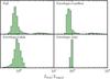 |
Fig. B.2 Distribution of Lbol/Linput for the different sets of models. Basic statistics of the distributions are listed in Table B.2. |
Appendix B.2: Luminosities
Photons escape more easily through low-density regions, where they are subjected to fewer scattering and absorption events, than through high-density regions, where the number of dust gains they can interact with is large. Consequently, one can expect the measured luminosity towards a source containing a disk or an outflow to depend on the viewing angle, whereas the measured luminosity towards a spherically symmetric source will be independent of the viewing angle.
Figure B.2 shows the distribution of Lbol/Linput for the different sets of radiative transfer models, where Lbol has been calculated by integrating over the synthetic SEDs. The most striking features are the narrowness of the envelope-only distribution, which is expected since the models are spherically symmetric, and the tail of high Lbol/Linput in the outflow models, which corresponds to viewing angles where one looks into the outflow.
 |
Fig. B.3 Size of the C18O-emitting region as function of the measured luminosity, Lbol, for the different sets of models. The errorbars indicate binned results, and the best fitting model, along with the 1σ uncertainty region is shown in green. Equation (B.1)is shown as the grey dashed line. |
Table B.2 presents basic statistics of the four distributions in Fig. B.2. As evident from the numbers, the most extreme deviations from the input luminosity occur in models with outflows, when the viewing angle is aligned with the outflow. This extreme situation is comparatively uncommon, and we therefore exclude viewing angles along the outflow when calculating the mean, median and standard deviation of the distributions. On average, the measured luminosities are smaller than the input luminosities because edge-on viewing angles are more likely than face-on viewing angles and because of the finite size of the aperture, which excludes extended emission. The magnitude of the latter effect can be estimated by looking at the envelope-only models, which deviate at most by 15% from the input luminosity and typically by much less. The average luminosity is reduced by a larger factor when including an outflow than it is when including a disk. This stems from the fact that a large fraction of the radiation escapes through the outflow, reducing the bolometric luminosity measured through the remaining viewing angles. On the other hand, models that contain disks show broader distributions than models without (again, excluding viewing angles that are along the outflow). This stems from the fact that the measured bolometric luminosity varies more strongly with viewing angle for models that contain a disk relative to models that do not.
While extreme situations do occur, we find that the measured bolometric luminosities are, on average, reduced by 20% relative to the input luminosity, and that deviations from the input luminosity larger than a factor of 2 are rare. The notable exception regards systems that are viewed through the outflow, where the measured bolometric luminosity may be enhanced by as much as a factor of 7 relative to the input luminosity. We do not believe this to be a great concern for the objects in our observed sample, since this case is expected to be rare, and because the majority of the observed systems have identified outflows, which suggests edge-on geometries. Our results are also in qualitative agreement with previous studies (e.g. Whitney et al. 2003; Offner et al. 2012).
Appendix B.3: C18O-emitting region
We wish to calculate the sizes of the C18O-emitting regions in the radiative transfer models and evaluate how they depend on the protostellar luminosity by fitting them to a functional relationship like that in Eq. (B.1). As a first step, the synthetic moment-zero maps are Fourier transformed and sampled in the (u,v)-plane using the (u,v)-coverage of Per-emb 53 as a template. Noise with a standard deviation of 4 Jy km s-1 is subsequently added to the synthetic (u,v)-data, again based on estimates of the noise in the Per-emb 53 data. Two-dimensional Gaussians are fitted to the synthetic (u,v)-data. The MCMC method presented in Sect. 3 is not used to fit the data, as it would be impractical given the large number of models; instead we use a standard non-linear fitting algorithm and ensure that the fit converges to a reasonable result by giving good starting guesses. Finally, the measured sizes of the C18O-emitting regions are binned according to their input luminosity and the set of models they belong to. The binned data are fitted to a functional relationship of the form ![Mathematical equation: \appendix \setcounter{section}{2} \begin{eqnarray*} \textit{FWHM}_\mathrm{avg}\left(x\right) = \begin{cases} \textit{FWHM}\left(x\right) & \textrm{if} \quad \textit{FWHM}\left(x\right) > c \\[2mm] c & \textrm{if} \quad \textit{FWHM}\left(x\right) \leq c,\end{cases} \nonumber \end{eqnarray*}](/articles/aa/full_html/2017/06/aa29739-16/aa29739-16-eq203.png)
where  The constant, c, is included to account for the fact that noise and (u,v)-coverage limit the sizes of the extents that can be measured, and c is therefore an estimate of that limit. Note that because the fitting is done directly in the (u,v)-plane the value of c can be smaller than the size of the synthesised beam.
The results of the fitting procedure for the Tsub = 28 K models are presented in Fig. B.3. Although the fitted parameters vary somewhat between the different sets of models, they are generally consistent with each other within 2σ. This suggests that the inclusion of disks and outflows has little influence on the location of the CO ice line, something that is also confirmed in Fig. B.1. Naturally, the CO ice line extends to large radii inside the outflows, but since the densities are low, this has little effect on the emission. Comparing to Eq. (B.1), we see that the power law exponents, b, derived here are, on average, somewhat flatter. We attribute this difference to the fact that the synthetic observables used a realistic (u,v)-coverage, and have had noise added to them, making them resemble real observations more. The expression that is used to predict the expected size of the C18O-emitting region in the main paper is the one for the full models, and is given as  We also fit the full models calculated for a sublimation temperature of 21 K to the functional relationship. The result is equal to that for a sublimation temperature of 28 K, except that the angular coefficient, a, is increased to (1.64 ± 0.10) arcsec.
All Tables
All Figures
|
Fig. 1 C18O 2–1 spectra towards the peak of the integrated emission of the observed sources. The integration intervals used for producing the moment-zero maps in Fig. 2 are indicated by vertical dotted lines and run from −2.5σ to 2.5σ of the fitted Gaussians (black dashed lines). The numeric value in the top left corner of each panel is the integrated emission over the line. |
| In the text | |
|
Fig. 2 Maps of C18O 2–1 integrated emission (line contours) and 1.3 mm continuum emission (colour map). Contours are drawn starting from 3σ in steps of 6σ (see Table 2 for C18O and continuum 1σ rms sensitivities). Synthesised beams of the C18O and continuum emission are shown in the lower left corners as respectively black and a shaded ellipses. Note that the beam sizes only differ significantly for the targets where extended data is available for the C18O emission. The blue symbols mark the source positions from the VANDAM survey (Tobin et al. 2016), with crosses indicating single protostars and triangles indicating multiple systems with projected separations <0.8′′. |
| In the text | |
|
Fig. 3 Examples of posterior parameter distributions of three fitted parameters towards Per-emb 1. The green lines represent the medians of the distributions and the shaded areas the 1σ uncertainty region. The median value and uncertainty are printed in the upper right corner of each panel. |
| In the text | |
|
Fig. 4 (u,v)-amplitude plots of the integrated C18O emission towards the sources in the observed sample. The grey dotted histograms in each panel indicate the expected amplitude in the absence of any source emission. The solid green line in each panel represents the best fitting Gaussian, while the shaded region indicates the 1σ uncertainty region of the fit. The vertical axis of each panel has been scaled to the Gaussian’s peak flux, whose value is printed in the upper right. The grey dashed lines indicate the 15 kλ lower boundary of the fit. Panels where the (u,v)-amplitudes have been plotted in grey indicate objects whose fits have been rejected (see text for details). |
| In the text | |
|
Fig. 5 Measured C18O extents versus the current (bolometric) luminosity. Triangular symbols represent sources that are associated with a companion protostar at a projected distance <0.8′′. The error-bars indicate the statistical uncertainties of the measurements listed in Table 3. The uncertainties of the luminosities are not shown to avoid cluttering the diagram, but they are small enough that they do not influence the conclusions. The solid line represents the expected CO extent given the current luminosity and a CO sublimation temperature of 28 K, while the dashed lines represent the expected CO extents for 10 and 100 times the current luminosity. The dash-dot line shows the expected CO extent for a sublimation temperature of 21 K. The horizontal dotted line at 1.4′′ indicates the lower limit of the extents that can be measured given the baseline coverage and sensitivity of the observations. |
| In the text | |
|
Fig. 6 Histograms of compact masses inferred from continuum flux densities at baselines >40 kλ. The black histograms show the full sample while the shaded histograms show only the sources that are identified as disk candidates in Table 4. The top panel shows uncorrected compact masses, while the bottom panel shows compact masses corrected for the envelope contribution using the method of Jørgensen et al. (2009). |
| In the text | |
|
Fig. 7 Comparison between observed and calculated (u,v)-amplitudes towards Per-emb 2 and 19. The calculated (u,v)-amplitudes are obtained from the axissymmetric models presented in Appendix B. In both cases we adopt an envelope power-law index of 1.5 and outflow half opening angle of 10◦. The adopted disk and envelope masses are printed in the panels and were motivated by the measured masses listed in Table 4. The model visibilities are averaged over 11 viewing angles and are shown as solid lines with shaded 1σ uncertainty regions. To account for the degeneracy between the assumed model masses and CO abundances, the model visibilities are normalised to the integrated single-dish flux density of each of the sources. The flux densities were estimated by convolving the moment-zero maps with a 20′′ Gaussian beam before reading the flux density at the source position. The red and blue model visibilities show the expected (u,v)-amplitudes for the current luminosity and for the luminosity needed to provide a good fit to the measured data. Panels to the left adopt a sublimation temperature of 28 K while panels to the right assume a sublimation temperature of 21 K. |
| In the text | |
|
Fig. 8 Top: cumulative distribution function of the difference between the Gaussian and outflow position angles. The dotted line shows a uniform distribution expected for a random relative orientation. Bottom: FWHMmajor/FWHMminor versus relative position angle. |
| In the text | |
|
Fig. 9 Corrected Mcompact (column marked “c” in Table 4) versus |
| In the text | |
|
Fig. A.1 (u,v)-amplitude plots of the integrated C18O emission towards the sources in the JVWB15 sample. The solid green line in each panel is the best fitting Gaussian, while the shaded region indicates the 1σ uncertainty region of the fit. The vertical axis of each panel has been scaled to the peak flux of the Gaussian fit, whose value is printed in the upper right. The grey dashed lines indicates the 15 kλ lower boundary of the fit. |
| In the text | |
|
Fig. B.1 Density cross-section of one of the full radiative transfer models. Both panels show the same model, but the right panel is zoomed in relative to the left. The model has parameters Mdisk = 0.1 M⊙, Menv = 1 M⊙, p = 1.5, |
| In the text | |
|
Fig. B.2 Distribution of Lbol/Linput for the different sets of models. Basic statistics of the distributions are listed in Table B.2. |
| In the text | |
|
Fig. B.3 Size of the C18O-emitting region as function of the measured luminosity, Lbol, for the different sets of models. The errorbars indicate binned results, and the best fitting model, along with the 1σ uncertainty region is shown in green. Equation (B.1)is shown as the grey dashed line. |
| In the text | |
Current usage metrics show cumulative count of Article Views (full-text article views including HTML views, PDF and ePub downloads, according to the available data) and Abstracts Views on Vision4Press platform.
Data correspond to usage on the plateform after 2015. The current usage metrics is available 48-96 hours after online publication and is updated daily on week days.
Initial download of the metrics may take a while.