| Issue |
A&A
Volume 600, April 2017
|
|
|---|---|---|
| Article Number | A137 | |
| Number of page(s) | 13 | |
| Section | Stellar atmospheres | |
| DOI | https://doi.org/10.1051/0004-6361/201629594 | |
| Published online | 14 April 2017 | |
Global 3D radiation-hydrodynamics models of AGB stars
Effects of convection and radial pulsations on atmospheric structures
Division of Astronomy and Space Physics, Department of Physics and Astronomy, Uppsala University, Box 516, 751 20 Uppsala, Sweden
e-mail: This email address is being protected from spambots. You need JavaScript enabled to view it.
Received: 26 August 2016
Accepted: 5 February 2017
Abstract
Context. Observations of asymptotic giant branch (AGB) stars with increasing spatial resolution reveal new layers of complexity of atmospheric processes on a variety of scales.
Aims. To analyze the physical mechanisms that cause asymmetries and surface structures in observed images, we use detailed 3D dynamical simulations of AGB stars; these simulations self-consistently describe convection and pulsations.
Methods. We used the CO5BOLD radiation-hydrodynamics code to produce an exploratory grid of global “star-in-a-box” models of the outer convective envelope and the inner atmosphere of AGB stars to study convection, pulsations, and shock waves and their dependence on stellar and numerical parameters.
Results. The model dynamics are governed by the interaction of long-lasting giant convection cells, short-lived surface granules, and strong, radial, fundamental-mode pulsations. Radial pulsations and shorter wavelength, traveling, acoustic waves induce shocks on various scales in the atmosphere. Convection, waves, and shocks all contribute to the dynamical pressure and, thus, to an increase of the stellar radius and to a levitation of material into layers where dust can form. Consequently, the resulting relation of pulsation period and stellar radius is shifted toward larger radii compared to that of non-linear 1D models. The dependence of pulsation period on luminosity agrees well with observed relations. The interaction of the pulsation mode with the non-stationary convective flow causes occasional amplitude changes and phase shifts. The regularity of the pulsations decreases with decreasing gravity as the relative size of convection cells increases. The model stars do not have a well-defined surface. Instead, the light is emitted from a very extended inhomogeneous atmosphere with a complex dynamic pattern of high-contrast features.
Conclusions. Our models self-consistently describe convection, convectively generated acoustic noise, fundamental-mode radial pulsations, and atmospheric shocks of various scales, which give rise to complex changing structures in the atmospheres of AGB stars.
Key words: convection / shock waves / methods: numerical / stars: AGB and post-AGB / stars: atmospheres / stars: oscillations
© ESO, 2017
1. Introduction
Variability with typical periods of 100–1000 days is a characteristic feature of stars on the asymptotic giant branch (AGB). The pronounced changes of the stellar luminosity are generally attributed to low-order large-amplitude pulsations. Various correlations between pulsation properties and stellar parameters have been derived from observations, for example, period-luminosity (P-L) relations. Evolved AGB stars, known as Mira variables, follow a linear P-L relation, similar to that of Cepheids, where a larger luminosity results in a longer period (see, e.g., Whitelock et al. 2008, 2009). Less evolved AGB stars fall on a series of P-L sequences, parallel to the sequence of Mira stars (Wood et al. 1999; Wood 2015). These sequences are interpreted as representing stars pulsating in various modes, with Mira variables pulsating in the fundamental mode while low-amplitude variables pulsate in overtones.
Pulsation and convection seem to play a decisive role in the heavy mass loss experienced by AGB stars. According to the standard picture, the observed outflows – with typical velocities of 5–20 km s-1 and mass loss rates in the range of 10-8–10-4M⊙ yr-1 – are accelerated by radiative pressure on dust grains, which are formed at about 2–3 stellar radii. Pulsations and non-stationary convective flows trigger strong atmospheric shock waves, which lift gas out to distances where temperatures are low enough and gas densities are sufficiently high to allow for the condensation of dust particles (for a recent review on this mass loss scenario, see, e.g., Höfner 2015).
Classically, variable stars have been analyzed via their light curves, which have been obtained for a large sample of objects and are usually regular for evolved AGB stars. However, high-resolution observations of nearby stars reveal complex irregular structures and dynamical phenomena on various spatial and temporal scales.
In the case of Mira (o Cet), Karovska et al. (1991) used speckle interferometry with various telescopes to detect asymmetries in the extended atmosphere that changed over time. Later, Karovska et al. (1997) speculated that the asymmetries detected with the Faint Object Camera on the Hubble Space Telescope (HST) in the UV and optical might be due to spots or non-radial pulsations. Lopez et al. (1997) found a best fit to observations in the IR taken with the Infrared Spatial Interferometer (ISI) by models with inhomogeneities or clumps. Chandler et al. (2007) presented a number of explanations for their ISI observations, among them shock waves and non-uniform dust formation. Recently, Stewart et al. (2016b) produced images of Mira by analyzing occultations by the rings of Saturn observed with the Cassini spacecraft showing layers and asymmetries in the stellar atmosphere.
Nevertheless, some phenomena may not be intrinsic to the star itself, since Mira is part of a binary system and the complex large-scale structure of the envelope may be attributed to wind-wind interaction (Ramstedt et al. 2014).
However, similar clumpy and non-spherical structures can be found around other AGB stars. For instance, very recently, Ohnaka et al. (2016) observed the semi-regular (type a) star W Hya with VLT/SPHERE-ZIMPOL and VLTI/AMBER and find supporting evidence for clumpy dust clouds caused by pulsations and large convective cells, as predicted by 3D simulations for AGB stars (Freytag & Höfner 2008).
A large number of observations exist of the carbon star IRC+10216 (CW Leo), starting with the first detection of a bipolar asymmetry in coronographic images by Kastner & Weintraub (1994). Haniff & Buscher (1998) attribute asymmetries in diffraction-limited interferometric images to envelope clearing along a bipolar axis. Weigelt et al. (1998) used speckle-masking interferometry with the SAO 6 m telescope to find a clumpy dust shell, that was considered as direct evidence for an inhomogeneous mass-loss process caused large-scale surface convection-cells, whose presence was suggested by Schwarzschild (1975). Recently, Stewart et al. (2016a) investigated the dynamical evolution of dust clouds in images reconstructed from aperture-masking interferometric observations using the Keck and VLT and from occultation measurements by Cassini, resulting in a complete change in the asymmetry and distribution of the clumps compared to the observations about 20 yr earlier by Kastner & Weintraub (1994), Haniff & Buscher (1998), and Weigelt et al. (1998).
The reason for these observed asymmetries could be the underlying irregular global convective flows in AGB stars, although the star itself or the stellar surface are not directly visible.
A realistic modeling of the underlying physical processes is a notoriously difficult problem and theoretical studies found in the literature are usually restricted to 1D simulations. Still, dynamical 1D atmosphere and wind models have been used successfully to explore the basic dust-driven mass-loss process, relying on a parameterized description of sub-photospheric velocities due to radial pulsations (so-called piston models; see, e.g., Bowen 1988; Fleischer et al. 1992; Winters et al. 2000; Höfner et al. 2003; Jeong et al. 2003; Höfner 2008). Mass loss rates and wind velocities along with spectral energy distributions, variations of photometric colors with pulsation phase, and other observable properties, resulting from the latest generation of such time-dependent atmosphere and wind models computed with the DARWIN code, show good agreement with observations (Nowotny et al. 2010; Eriksson et al. 2014; Bladh et al. 2015; Höfner et al. 2016).
One-dimensional CODEX models of gas dynamics in the stellar interior and atmosphere, simulating (radial) Mira-type pulsations as self-excited oscillations and following the propagation of the resulting shock waves through the stellar atmosphere, have been presented by Ireland et al. (2008, 2011), for instance.
Despite their success in reproducing various observational results, 1D dynamical models are not sufficient to give a comprehensive picture of the physical processes leading to mass loss on the AGB. These 1D models require a number of free parameters that have to be carefully adjusted, for example, to describe the variable inner boundary (“piston”) in dynamical atmosphere and wind models or the time-dependent extension of the mixing-length theory (MLT) in non-linear pulsation models. Further, such models cannot simulate intrinsically 3D phenomena such as stellar convection and they therefore cannot describe the giant convection cells that are presumably giving rise to the non-spherical and clumpy morphology of the atmosphere.
Turbulent flows, in general, and stellar convection, in particular, are known to produce acoustic waves if the Mach number is sufficiently large (Lighthill 1952). This excitation process has been studied with local 3D radiation-hydrodynamics simulations for the case of the Sun, for example, by Nordlund & Stein (2001) and Stein & Nordlund (2001). The steepening of these waves while traveling upward into the chromosphere was investigated by Wedemeyer et al. (2004). Such local 3D radiation-hydrodynamics simulations have been used for decades to model small patches on the surface of (more or less) solar-type stars. Now a number of grids produced by different groups with various codes are available (Ludwig et al. 2009; Magic et al. 2013; Trampedach et al. 2013; Beeck et al. 2013), which also extend to the regime of white dwarfs (Tremblay et al. 2015).
In contrast to these compact types of stars, giants might be covered by only a small number of huge convective cells, as suggested by Stothers & Leung (1971) as an explanation for irregularities in the light curves. Schwarzschild (1975) argued that, if the size of surface convection cells is governed by some characteristic length scale, such as the density scale height, the counterpart of small solar granules should be huge convective structures on giants. Consequently, these stars should produce large-scale acoustic waves. Surface convection and associated waves, pulsation, and shocks have been investigated with global 3D radiation-hydrodynamics simulations with the CO5BOLD code (Freytag et al. 2012), both for the case of red supergiants, for instance, by Freytag et al. (2002) and Chiavassa et al. (2009), and with an exploratory study for an AGB star by Freytag & Höfner (2008). These studies confirm the existence of large-scale convection cells and acoustic waves.
In this paper, we present the first grid of AGB star models produced with a new, improved version of CO5BOLD. We analyze the dependence of the properties of convection and pulsations on stellar parameters and also look at the influence of rotation.
Basic model parameters.
2. Setup of global AGB star models with CO5BOLD
Following our earlier work (Freytag & Höfner 2008), we present new radiation-hydrodynamics simulations of AGB stars with CO5BOLD (Freytag et al. 2012). Improvements regarding the accuracy and stability of the hydrodynamics solver are outlined in Freytag (2013).
The CO5BOLD code solves the coupled non-linear equations of compressible hydrodynamics (with an approximate Roe solver) and non-local radiative energy transfer (for global models with a short-characteristics scheme) in the presence of a fixed external gravitational field. The numerical grid is Cartesian. In all models presented here, the computational domain and all individual grid cells are cubical. The tabulated equation of state takes the ionization of hydrogen and helium and the formation of H2 molecules into account. It is assumed that solar abundances are appropriate for M-type AGB stars. The tabulated gray opacities (very similar to those used in Freytag & Höfner 2008) are merged from Phoenix (Hauschildt et al. 1997) and OPAL (Iglesias et al. 1992) data at around 12 000 K, with a slight reduction in the very cool layers (that are hardly reached in the current model grid) to remove any influence of dust onto the opacities. There are no source terms or dedicated opacities for dust: no dust is included in any of the current models in contrast to the two old models st28gm06n05 and n06.
The gravitational potential is spherically symmetric (see Eq. (41) in Freytag et al. 2012), corresponding to a 1 M⊙ core in the outer layers and smoothed in the center at r ≲ R0 = 78 R⊙ (see Fig. 4 in Freytag & Höfner 2008). The tiny central nuclear-reaction region cannot possibly be resolved with grid cells of constant size. Instead, in the smoothed-core region, a source term feeds in energy corresponding to 5000, 7000, or 10 000 L⊙. A drag force is only active in this core to prevent dipolar flows traversing the entire star. All outer boundaries are open for the flow of matter and for radiation.
The start models for the first AGB simulations presented in Freytag & Höfner (2008) were based on hydrostatic 1D stratifications (see Fig. 1 of Chiavassa et al. 2011a, showing images from the initial phase of a simulation of a red supergiant started this way). All later AGB models were derived from a predecessor 3D model by either refining or coarsening the numerical grid, adding or removing grid layers to change the size of the computational box, increasing or decreasing the core luminosity in time in steps of 1000 L⊙, or by modifying the density in each grid cells in each time step by a tiny amount to change the initial to the final envelope mass. While the initial adjustment time lasted typically a few years, the typical total simulation time span is 109 s (just above 30 yr). We monitored the time evolution of several quantities, for instance, the total emerging luminosity and the mass density in the very center, to ensure that the models are well relaxed when we compute averaged quantities for further analysis (see below).
Table 1 and Fig. 1 give an overview of the simulations split into three groups: old models from Freytag & Höfner (2008), new test models used for parameter studies (including rotation rate), and a grid of models with different stellar parameters.
While, for instance, the mass M⋆ (controlling the gravitational potential), the resolution and the extent of the numerical grid, and the rotation rate are pre-chosen fixed parameters (second group of columns in Table 1), other model properties are determined after a simulation is finished (third group in Table 1). The stated stellar luminosity is a time average of the luminosity for each “fine” snapshot without the full 3D information, but with lots of preprocessed – and thus compressed – data, saved every 250 000 s ≈3 d. The envelope mass Menv, however, is calculated from the integrated density for each fine snapshot averaged over time. Nevertheless, the radius is more difficult to determine and less well defined. The radius is chosen as that point R⋆ where the spherically (abbreviated as ⟨ . ⟩ Ω) and temporally (denoted as ⟨ . ⟩ t) averaged temperature and the average luminosity ⟨ L ⟩ Ω,t fulfill ⟨ L ⟩ Ω,t = . Then, effective temperature and surface gravity follow.
To investigate purely radial motions we take averages over spherical shells for each fine snapshot for the radial mass flux ⟨ ρvradial ⟩ Ω(r,t) and the mass density ⟨ ρ ⟩ Ω(r,t) and take the ratio as the radial velocity, which is now a function ⟨ vradial ⟩ (r,t) of radial distance and time. The derivation of the pulsation quantities Ppuls and σpuls of Table 1 is described in Sect. 3.3.
3. Results
3.1. General dynamics and comparison to old models
The time evolution of various quantities can be followed in the snapshot sequences in Figs. 2 and 3; the plots of radial velocity as function of radius and time are shown in Fig. 4 (along a particular radius vector: vradial(r,t)) and Fig. 5 (averaged over spheres: ⟨ vradial ⟩ (r,t)).
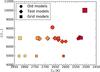 |
Fig. 1 Luminosity and effective temperature of all models. The colors of the markers represent the temperature of the models while the size of the markers represent the luminosity. The shape of the markers indicates which group in Table 1 the models belong to; the “old” models from (Freytag & Höfner 2008) are circles, the “test” models with varied numerical parameters are diamonds, and the “grid” models with different stellar parameters are squares. |
3.2. Convective motions
The convection zone is essentially indicated by the bright (high entropy) irregular inner part of the entropy snapshots in Fig. 2 with a radius around 300 R⊙, which is smaller than the inferred stellar radius of R⋆ = 371 R⊙ given in Table 1; i.e., light is emitted from layers further out. The drop in entropy at the top of the convective layers is accompanied by a drop in temperature and even a thin density-inversion layer.
Huge convective cells can span 90 degrees or more in the cross sections, which is in line with extrapolations by Schwarzschild (1975) from solar granulation. The cells are outlined by non-stationary downdrafts reaching from the surface of the convection zone to the center of the model star. While the flow travel time from the surface to the center is around half a year, the convective cells can have a lifetime of many years, causing long intervals of one preferred flow direction in the convection zone in Fig. 4. These downdrafts even have a tendency to traverse the artificial stellar core and to create a global dipolar flow field. However, in the (non-rotating) models presented here, the drag force, which is somewhat arbitrarily applied in the stellar core, prevents these flows.
The surface of the convection zone appears corrugated; this is caused by many smaller short-lived convection cells close to the surface. Their number increases with numerical resolution, as a comparison of Fig. 2 with Fig. 1 of Freytag & Höfner (2008) reveals.
Simulations of red supergiants (RSGs) with CO5BOLD (Freytag et al. 2002; Chiavassa et al. 2009; Arroyo-Torres et al. 2015) show large-scale convection cells as well. But for RSGs the ratio of surface pressure scale height, and therefore the size of the convective structures and the local radius fluctuations, to radius is smaller than for AGB stars, so that RSGs appear more spherical.
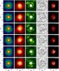 |
Fig. 2 Time sequences (for the extended model st28gm06n25) of temperature slices, density slices, entropy slices, pseudo-streamlines (integrated over about 3 months), and bolometric intensity maps, where black corresponds to zero intensity. The snapshots are nearly 3 months apart (see the counter in the right-most panels), so that the entire sequence covers about one pulsational cycle. The color scales are kept the same for all snapshots. This figure can be directly compared to Fig. 1 of Freytag & Höfner (2008). |
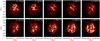 |
Fig. 3 Time sequence (for the standard model st28gm06n26) of bolometric intensity maps, where black corresponds to zero intensity. The snapshots are about 1 month apart to demonstrate the relative short timescale for changes of the small surface features. |
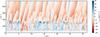 |
Fig. 4 Plot (for the standard model st28gm06n26) of radial velocity vradial(r,t) for all grid points in one column from the center to the side of the computational box for the entire simulation time. Blue indicates outward and red inward flow. |
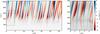 |
Fig. 5 Examples for the standard model st28gm06n26: Left: the spherically averaged radial velocity ⟨ vradial ⟩ (r,t) for the full run time and radial distance. The different colors show the average vertical velocity at that time and radial distance. Right: part of the velocity field from the right image, indicated with the rectangle with mass-shell movements plotted as iso-mass contour lines. |
3.3. Pulsations
3.3.1. Exploring the pulsation mode and period
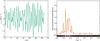 |
Fig. 6 Examples for the standard model st28gm06n26: Left: the vertical velocity at a constant r = 301 R⊙, over 30 yr. Right: the power spectrum of the vertical velocity, shown to the left, showing the clearly dominant frequency. At the bottom of the panel, the density plot for this power spectrum is shown. This type of data is used in Fig. 7 for all radial points. |
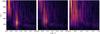 |
Fig. 7 Power spectra derived from the velocity fields of three different models, mapped over frequency and radial distance. For easier comparison all the different power spectra have been area normalized. Left: model st29gm04n001, the hottest and smallest model, is shown. Middle: the standard model st28gm06n26 is shown. Right: model st28gm07n001, the coolest and most luminous model with the largest radius, is shown. |
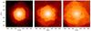 |
Fig. 8 Density slices for the three models used in Fig. 7. The range used for all color tables is –16 ≤ log ρ ≤ –6.7. |
The density snapshots in Fig. 2 show irregular structures with convection cells in the interior and a network of shocks in the atmosphere. To investigate purely radial motions we consider the density-weighted spherical average of the radial velocity ⟨ vradial ⟩ (r,t) as described in Sect. 2 and plotted in Fig. 5 for the standard model st28gm06n26.
The behavior of the inner part of the model differs from that of the atmosphere, which is particularly evident in Fig. 5. Below about 400 R⊙ (the nominal radius is R⋆ = 371 R⊙), the pulsation is rather regular and coherent over all layers, close to a standing wave. The fundamental mode dominates as there are no nodes in the velocity map. In the outer layers, however, the slopes in the velocity map indicate propagating shock waves (see Sect. 3.4).
In the right panel in Fig. 5, a close-up of part of the velocity field is shown, with movements of mass shells overlaid, analogous to plots for the 1D models, for example, in Höfner et al. (2003) or Nowotny et al. (2010). The amplitude of the 3D mass-shell oscillations is smaller than for corresponding 1D models by a factor of two or more. This is at least partly due to the averaging over the full 3D model, which smoothes the amplitude as the shock waves are not exactly spherical.
To quantify the periodic behavior a Fourier analysis is performed using the averaged radial velocity ⟨ vradial ⟩ (r,t). An example for r = 301 R⊙ is shown in the left panel of Fig. 6, again for model st28gm06n26 with the corresponding power spectrum in the right panel. Frequencies around 0.6 yr-1 dominate.
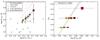 |
Fig. 9 Left: logarithm of the period of the models plotted against the logarithm of the resulting radius with three different period-radius relations plotted. The green line indicates period-radius relations from this work, the orange dashed line indicates Wood (1990), and the purple dotted line indicates Fox & Wood (1982) for M = 1 M⊙. The error bars of the pulsation period of the models refer to the width of the peak in the power spectrum, that is, larger than the uncertainty of the period. The statistical error in the model radius is small. The typical error in the observed radii is about 31% due to uncertainties in the parallax. The crosses and circles are observations of C stars and M stars, respectively, with radius from the CHARM2 catalog (Richichi et al. 2005) and periods from GCVS catalog (Samus et al. 2009). Only stars with measured parallaxes were picked so that the distance determination is independent of the measured period (Ramstedt & Olofsson 2014). Right: the absolute magnitude against the logarithm of the period for all models. The error in the absolute magnitude is only due to the finite simulation time and is tiny (a few mmag). The line is taken from Whitelock et al. (2009) and is the P-L relation for AGB stars in the LMC, where the gray area is the 1σ error of the fit to the observations. |
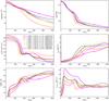 |
Fig. 10 Plots of selected quantities, averaged over spherical shells and time vs. radii for all grid models. The plus signs roughly indicate the depth with τRoss = 1. Top left: logarithm of the mass density ρ. Top right: logarithm of the temperature T. Center left: entropy per mass unit s. Center right: temporal rms value of the spherically averaged radial velocity (includes mostly contributions from the radial pulsations). Bottom left: logarithm of the ratio of dynamical pressure Pdyn and gas pressure P. Bottom right: temporal and spatial rms value of the radial velocity (includes contributions both from convection and radial pulsations). |
To explore the behavior all through the star the power spectra of the averaged radial velocity ⟨ vradial ⟩ (r,t) at all radii are plotted in the middle panel of Fig. 7. Again the two different behaviors in the inner and outer layers of the model are evident. There is a dominant frequency in the stellar interior, as suspected from Fig. 5. However, the outer layers beyond r ~ 400 R⊙ no longer pulsate with the same period as the interior of the star. Lower frequency signals become more prominent and beyond r ~ 600 R⊙ (far out in the shock-dominated atmosphere), and the frequency with the largest amplitude is significantly smaller than that of the interior of the star.
In the power spectra of models with different stellar parameters in Fig. 7, the dominant mode generally becomes more diffuse with increasing radius of the model. For more compact models, for instance model st29gm04n001 with R⋆ = 294 R⊙ in the left panel in Fig. 7, there is a very clear dominant mode in the interior. For the standard model (middle panel in Fig. 7 with radius R⋆ = 371 R⊙) there is still a dominant frequency, but the spread around this frequency is larger. For the largest model (model st28gm07n001 with R⋆ = 531 R⊙ in the right panel in Fig. 7), the power seems to be equally distributed over a large frequency range, lacking the clear dominant frequency that is present in the two other models.
To find the dominant frequency and therefore the pulsation period and to investigate the spread in frequencies, the area-normalized power spectra of the radial velocities for radial distances r = 0.5–1 R⋆ were added. For instance, this corresponds to radial points in the range r = 185.5–371 R⊙ for the standard model. A Gaussian distribution was fitted in the frequency domain containing the strongest signal. The central value for the fit for each model is taken as the dominant frequency fdom, while the spread in frequencies is represented by the standard deviation σpuls. The resulting periods Ppuls = 1 /fdom and spreads σpuls are listed in Table 1 and plotted in Fig. 9, where the colors of the squares represent the temperature with lighter colors indicating higher temperature and the size represents the luminosity of the model, as seen in Fig. 1.
3.3.2. Excitation mechanism
The irregular spread of the mode frequencies in Fig. 7 is likely due to interactions between the pulsations and large-scale convective motions causing occasional amplitude changes and phase shifts. With larger radii, the convective cells increase further in relative size resulting in stronger disturbances of the pulsation mode. Within a luminosity group, the frequency spread grows with decreasing radius, which is likely due to the increase of convective velocities with increasing effective temperature; cf. the bottom right panel in Fig. 10.
The power spectra in Fig. 7 can be compared to the power spectrum derived from a local solar model in Fig. 3 of Stein & Nordlund (2001). The similarity is an indication of a common excitation mechanism.
Analyzing light curves, Christensen-Dalsgaard et al. (2001) attributed oscillations in semi-regular variables to stochastic excitation by convection. Bedding et al. (2005) distinguished several cases. These authors attributed large phase fluctuations in the light curve of the semi-regular star W Cyg to stochastic excitation, whereas the very stable phase of the true Mira star X Cam was found to be consistent with the excitation by the κ mechanism. L2 Pup was classified as an intermediate case in which both mechanisms play a role.
Analyzing the work integral in 1D pulsation models, Lattanzio & Wood (2004) concluded that the driving mechanism, at least for Mira variables, is likely a κ mechanism acting in the partial hydrogen and helium I ionization zone.
Our grid of 3D models, which only covers a small part of the entire range of the AGB star parameters, already shows a range of different behaviors of the oscillations (see Fig. 7 and the discussion in the previous section), where the trend clearly points to the role of convection and the size of the convective cells for the excitation of, or at least interaction with, the pulsation. The non-stationary transonic convective flows with Mach numbers, which in the downdrafts often exceed unity, produce acoustic noise as described by Lighthill (1952) for turbulent flows. This excitation mechanism has been investigated for instance by Nordlund & Stein (2001) and Stein & Nordlund (2001) with local 3D radiation-hydrodynamics simulations of solar granulation. The Mach numbers in near-surface convective flows of AGB stars can be even larger causing more efficient wave excitation (Lighthill 1952). As the relative sizes of the exciting convective structures are very large, the generated waves have much lower wave numbers than on the Sun.
To check that the radial pulsations are not just (long-lasting) transient phenomena introduced by the initial conditions, we added a strong (purely artificial) drag force in the entire model volume. This drag force reduced the amplitude of the pulsations (and the convective flows) but did not lead to an exponential decay of the radial mode, indicating that an efficient mode-excitation mechanism must be at work.
In the models of Freytag & Höfner (2008), these pulsations existed and their amplitude was extracted as a description of the piston boundary in 1D models. However, the global pulsations were harder to distinguish from the local shock network because of the lower numerical resolution; this led to larger sizes of convective and wave structures and shorter time sequences, which made a Fourier analysis less reliable than what is possible for the current model grid.
3.3.3. Comparison with 1D models and observations
As has been pointed out by Fox & Wood (1982) and Wood (1990), AGB stars do not seem to follow the simple period-mean-density relation, 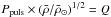 , where Q is the pulsation constant. This is not very surprising because the derivation of the period-mean-density relation relies on the assumptions that displacements are adiabatic and non-linear effects are small, both of which are probably incorrect for AGB stars. Instead, these works, using 1D pulsation models, find that Ppuls ∝
  with α ~ 1.5–2 and β ~ 0.5–1. The period-radius relation for our models with a fixed mass M⋆ = 1 M⊙ is compared to that of Fox & Wood (1982) and Wood (1990) in the left panel of Fig. 9. We find
  (1)which gives generally a larger radius for a given period. There might be several reasons for this difference in addition to uncertainties in the 1D models.
There is a contribution to the extension of the atmosphere of the 3D models (see Sect. 4.2) due to the convectively generated, small-scale shocks (see Sect. 3.4) that do not exist in the 1D models. This would affect the photospheric radius but not the pulsation period if the shocks occur above the top of the acoustic cavity. This contribution might even lower the slope because the largest models have the most extended atmospheres. The convective envelope is not in hydrostatic equilibrium but is affected by the convective dynamical pressure as well. In addition, the treatment of the artificial core in the 3D models might play a role. However, the effect should be small because the sound-crossing time for the core, and therefore the contribution to the period, is relatively small. Finally, there is some uncertainty in the determination of radius and period.
In the left panel of Fig. 9, observations of the radii for different AGB stars are plotted against the periods with C stars shown as crosses and M stars as circles. The diameter observations are from Richichi et al. (2005), periods from Samus et al. (2009), and parallaxes from van Leeuwen (2007). The 3D models agree fairly well with observations, especially the lower luminosity models. The period-radius relation from the 1D models might produce periods that are too long for the range of radii explored by the 3D models when compared to observations. However, 1D models predict that altering the mass leads to a change of the period-radius relation. While only the relations for 1 M⊙ are plotted here for direct comparison to the results from the 3D models, 1D models from Fox & Wood (1982) can reach the shorter periods, if the mass of the models is increased.
It is difficult to draw any final conclusion as the errors in determining fundamental parameters for field AGB stars are very large. The uncertainties in observed absolute magnitudes originate mainly from uncertainties in the parallaxes, which are difficult to determine for AGB stars as the photo-centers of these stars are variable (for a statistical analysis of photocentric variability, see Ludwig 2006; Chiavassa et al. 2011b). Also, the uncertainty of observations of the radii of AGB stars is fairly large, sometimes on the order of the stellar radius. In addition, the radius varies significantly during a pulsation cycle and the phases are not always well known. Here, we use the mean radius as reference. However, the radius varies by around 20% during one pulsation period for our models.
It is also likely that the stellar masses affect the period-radius relation. However, unless there are well-observed companion stars, it is usually not possible to determine masses from observations. A theoretical prediction of the effect of different masses is not yet possible, as all the models in the current grid have a mass of 1 M⊙.
A property that is better constrained by observation is the P-L relation, which has been extensively studied. A comparison between the 3D models and observation by Whitelock et al. (2009) is shown in the right panel of Fig. 9. The models from the grid follow a trend of brighter absolute magnitude with larger period, which is qualitatively similar to that of the observations. There is, however, a spread in the periods because of the different effective temperatures and radii for a given luminosity, giving constraints for our – so far a bit arbitrary – choice of the combination of the main control parameters M⋆, Menv, L⋆, and metallicity of the 3D models.
3.4. Atmospheres with networks of shocks
The steepening of acoustic waves in the solar chromosphere and the transformation into a network of shocks was modeled by Wedemeyer et al. (2004) and Muthsam et al. (2007). AGB stars have a larger temperature drop from the convection zone to the atmosphere (cf. Figs. 5 and 6 in Freytag & Chiavassa 2013, for a model sequence from the Sun with log g = 4.44 to a 5 M⊙ star with log g = –0.43) that is accompanied by a larger change in pressure or density scale height. This leads to a stronger compression and amplification of the waves in the cool atmosphere, so that the waves very early turn into shocks, leaving no room for an essentially undisturbed photosphere. Sound-speed variations, particularly at the rugged surface of the convection zone, and transonic convective flow speeds shape the waves and contribute to the generation of small-scale shock structures (at r > 300 R⊙ in Fig. 4), which give rise to ballistic gas motions with peak heights of a few ten to a few hundred solar radii. The strongest shocks can even leave the computational box.
The plot of entropy versus radius in Fig. 10 shows that part of the atmosphere is a zone of convective instability – with negative entropy gradient – separate from the normal interior convection zone. The image sequences in Fig. 2 and the plot of vradial(r,t) in Fig. 4 show a very different behavior of the two zones: only the inner zone is governed by the normal overturning motions, whereas propagating shocks dominate in the outer zone (as discussed in Sect. 3.3.1). But still, the convective instability might destabilize the shocks favoring a tendency toward smaller structures as seen in the intensity snapshots in Figs. 2 and 3. For models with L = 5000 L⊙, this instability zone lies two times further out relative to the stellar radius, compared to the higher luminosity models. Woitke (2006) showed that in 2D simulations of the atmosphere of an AGB star, where the radial stellar pulsation and inhomogeneities generated by convection are ignored and shocks are generated by an external κ mechanism, instabilities within the shock fronts can cause small-scale structures to form.
A combination of relatively small-scale acoustic noise and global, radial pulsations generates the network of shocks with a size spectrum regulated by several complex processes; a wave emitted from a small region close to the surface might turn into an expanding shock wave, which fills a large part of the atmosphere if the surrounding flow permits it. The overtaking and merging of shocks increases the typical size. On the other hand, large-scale waves in the interior are shaped by the convective background flow and sound-speed distribution and can become as rugged as the surface of the convection zone itself. And the convective instability in the atmosphere also favors small scales.
The shock fronts show up prominently in the density slices in Fig. 2 and are only occasionally visible in the temperature slices (e.g., in the upper left quadrant in the fourth row) because the radiative relaxation is fast enough to cool down the heated post-shock material to the local equilibrium value, even with the gray radiative transfer used. The radiative relaxation time decreases further when non-gray radiative transfer is employed (in a first simulation), essentially wiping out any temperature signature of the shocks. That might change again with a drastic increase in numerical resolution, which is currently not achievable.
While the temperature stratifications of the various models in Fig. 10 show many differences in the convection zone and inner atmosphere, they converge into one of three profiles in the outer atmosphere, depending only on stellar luminosity. This and the relatively small temperature fluctuations in the outer part of the temperature slices in Fig. 2 indicate that the thermal structure of the outer atmosphere is dominated by radiative processes and is not far from radiative equilibrium. The shocks show up in the velocities and the density but hardly in the temperature.
Expectedly, the size spectrum of the shocks is extended toward smaller scales with increasing resolution as a comparison of Fig. 2 of the current paper with Fig. 1 of Freytag & Höfner (2008) demonstrates.
3.5. Rotation
Rotation plays an important role in stellar activity and possibly also in the dynamics of stellar winds. The loss of angular momentum from magnetic coupling with the surroundings or from a wind likely slows down evolved stars considerably. Dorfi & Höfner (1996) performed 1D stationary-wind models of a 1 M⊙/2600 K/10 000 L⊙ AGB star and found that a rotation period of 40 yr modifies the isotropic mass loss marginally, while a period of 10 yr results in a drastic increase of the mass loss rate and causes a significant axial asymmetry of the wind.
In hydrodynamical simulations of convection in the interior of rotating stars, the Mach numbers are so low that the flow is essentially incompressible and the optical thickness of individual grid cells is so large that radiation transport is adequately described by the diffusion approximation.
However, these conditions are not met in the convective envelopes and surrounding atmospheres of AGB stars, where the numerical treatment in CO5BOLD (e.g., of non-local radiation transport and compressible hydrodynamics) is required, so we modified the CO5BOLD setup to account for rotation. While it is possible to just add a rotational velocity field to the initial model, we chose to perform the simulation in a corotating frame. A centrifugal potential is added to the gravitational potential. Before each hydrodynamics step the Coriolis force is applied, which just rotates the velocity vectors, but with twice the amount simply suggested by period and time step. The artificial drag force in the model core was chosen to act only radially so as not to affect the angular momentum. We computed a first exploratory pair of models with rotation periods of 20 and 10 yr (see Table 1). Longer periods would require even longer integration times. The Prot = 20 yr simulation was started from a snapshot from a non-rotating run, and the period was decreased (by increasing centrifugal potential and Coriolis force) gradually over a few stellar years to avoid transient oscillations due to a too rapid change of the potential.
As expected for slow rotators, where the rotational period is longer than typical convective turnover timescales, angular momentum is advected inward into a small region close to the core of the model (see Fig. 11). In spite of the drag force in the core, a global dipole flow develops with typical velocities in the atmosphere of vmeridional = 4 km s-1 (for st28gm06n29 with Prot = 20 yr) and vmeridional = 2.5 km s-1 (for st28gm06n30 with Prot = 10 yr).
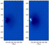 |
Fig. 11 Azimuthally and temporally averaged velocity fields for models st28gm06n29 (Prot = 20 yr, left) and st28gm06n30 (Prot = 10 yr, right). The color plot shows the angular momentum in the corotating frame; bright blue means rotation faster than the mean given by Prot, and dark blue means rotation slower than the mean. |
While the core generally rotates very rapidly, the part of the convection zone that is not close to the axis rotates slower than the nominal rate. Part of the material close to the core of the model with Prot = 20 yr even shows a slow retrograde rotation. However, all azimuthally averaged velocity components show large fluctuations and the averaging time or relaxation time for this model might not yet be sufficient.
The mean atmospheric stratification is affected by the rotating star: while the temperature stratification shows hardly any effect, the average density in the atmosphere increases with shorter rotation period (see Fig. 10).
Our rotating models have a number of shortcomings. The approximation of the smoothed stellar core plays a larger role than for purely convective (and pulsating) flows that are not rotating. Would the angular momentum in a real star be advected even further in and leave only a very slowly rotating convective envelope and atmosphere behind? What role would magnetic fields play in coupling the interior to the convective envelope? The outer boundaries might also influence the results because the slowly rotating atmosphere moves with respect to the computational box and might exchange angular momentum through the boundaries. Clearly, improved models need a larger computational domain and update of the treatment of the stellar core.
Still, the presented models support the results of Dorfi & Höfner (1996) that rotation in AGB stars – if the period is on the order of 20 yr or shorter – can influence the atmospheric velocity field and the wind, and might be responsible for the shapes of some planetary nebulae.
4. Discussion
4.1. Influence of numerical parameters
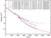 |
Fig. 12 Logarithm of the gas density averaged over spherical shells and time for six models. The ordering in the legend essentially corresponds to the order of the curves. The plus signs roughly indicate the depth with τRoss = 1. In the legend, the effective temperature, surface gravity, edge length of the computational box, number of grid points, and the name are given for each model. |
The current models have an improved resolution over those presented in Freytag & Höfner (2008) because of an increased number of grid points and a higher order reconstruction scheme of the hydrodynamics solver (Freytag 2013). While sub-surface convection cells and above-surface shocks show finer structures, there are no qualitative changes in the general results. Still, the newer models allow a better separation of the radial pulsation mode from the convective noise and also present a longer time base for the Fourier analysis.
The averaged density stratifications for selected models in Fig. 12 give an idea about the size of effects due to changes in numerical parameters. The two smallest and oldest models, n02 and n06 (referring to the last three letters of the model names), which were already used in Freytag & Höfner (2008), have the same resolution but different extensions of the computational box and agree well with each other. The same is true for the pair n24/n25 from the current “test” group of models, indicating that the box size does not have a major impact. The curves for n24 and our standard model n26 are indistinguishable. The difference is a change in the version of the code, which mainly entails a modification of the WENO scheme used for the high-order reconstruction in the hydrodynamics solver. We implemented a reduction of the order of the reconstruction, and therefore an increase in dissipation, in case of large Mach numbers or large gradients in pressure or entropy. The numerical resolution of model n16 was increased by a factor of 1.43 in each direction, compared to n13 with only a slight effect on the mean-density stratification.
The noticeable decrease of the density by about one order of magnitude in the outer layers from n13/n16 to n24/n25/n26 is caused by a change in the outer boundary conditions. Assuming a less steep density decrease while filling the ghost cells at the boundaries of the computational box induces a stronger infall of material in the phase between outward moving shocks and somewhat impedes propagation of the shocks, leading to lower averaged densities in the outer layers. An additional reduction might be due to a difference in the treatment of the velocity damping in the core region of the models, which prevents large-scale dipolar flows that could develop and dominate the entire convective envelope. Between the old models n02/n06 and the new models, there are differences in the envelope mass Menv and too many changes in the numerics to allow a disentanglement of the influence of individual settings.
4.2. Dynamical pressure
The bottom left panel in Fig. 10 shows the ratio of the radial component of the dynamical pressure and the gas pressure, both averaged over spheres and time,  /⟨ P ⟩ Ω,t. From the total dynamical pressure, we derive a density-weighted rms value of the radial velocities according to
  / ⟨ ρ ⟩ Ω,t)1/2, and the (smaller) contribution by the radial pulsations
 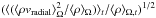 , plotted in the bottom right and the middle right panels, respectively.
In the convection zone, where the pressure ratio is below one, it already stays above 20% for a number of models for a large fraction of the radius. Thus, the dynamical pressure is not negligibly small and influences the stratification at least of the outer convective envelope. The peak of the radial velocities near the surface of the convection zone is accompanied by a peak in the pressure ratio and the dynamical pressure becomes even larger than the gas pressure.
Further out in the atmosphere, the dynamical pressure dominates over the gas pressure (radiation pressure is not included in the current models) by factor of 5 to 10. It significantly increases the density and pressure scale heights compared to the case with only gas pressure, causing a levitation of dense material into cool layers. This allows molecules to form and possibly creates a highly irregular, non-spherical, and dynamic version of a MOLsphere (an extended sphere around the star that is optically thick in molecular lines, for instance, due to water; see Tsuji 2000). In addition, the conditions become even sufficiently cool and dense for dust to form (see, e.g., Freytag & Höfner 2008). The contributions of purely radially symmetric motions (middle right panel in Fig. 10) and spatially fluctuating flows to the total radial velocities (bottom right panel in Fig. 10) are both significant, but only the radially symmetric motions can be accounted for by dynamical 1D models.
While we get very extended atmospheres in our models of AGB stars, Arroyo-Torres et al. (2015) concluded that for red supergiant stars (with much larger masses in the range 5–25 M⊙) the dynamical pressure in pulsating 1D models and the even larger dynamical pressure in 3D CO5BOLD models is not sufficient to enlarge the photosphere to the observed sizes.
4.3. Small-scale structures in the atmosphere
We presented some observations (e.g., by VLT/SPHERE, HST, VLTI, and various other interferometers, or with the Cassini spacecraft) of asymmetries and clumps in the dust envelopes of near-by AGB stars in the Introduction.
The bolometric-intensity maps in Figs. 2 and 3 derived from the 3D models show that the smallest scale patterns change on timescales of less than a month, while intensity changes of larger areas occur on timescales of about a year.
The surface of the normal stellar convection zone (see Sect. 3.2) sits too deep to directly affect the emergent intensity: surface granules and larger convection cells themselves are not observable. Instead, the visible structures are caused by shocks on various scales. However, as described in Sect. 3.4, the shocks are shaped by the underlying convective structures. A dimming and brightening of a large area (see Fig. 3) might well indirectly reflect the dynamics of the convection.
A detailed comparison of results from the 3D models with observations has to await simulations with non-gray opacities and a detailed treatment of dust as well as time series of high-angular-resolution observations.
4.4. Characteristic timescales
A comparison of the pulsation period with the various typical timescales of convective structures (see Sect. 3.2) gives 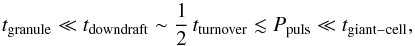 (2)i.e., that the granules adjust to the pulsation whereas the giant cells are more or less frozen in. However, a restructuring of the giant cells can lead to a variation of the detailed pulsation behavior on rather long timescales of several years. The strongest interaction is to be expected between pulsations and downdrafts. There is no such thing as “the” convective timescale.
5. Conclusions
We presented a first exploratory grid of 3D radiation-hydrodynamics models of AGB stars computed with a new version of CO5BOLD, which is improved in terms of accuracy, stability, and boundary treatment compared to the version used for the simulations presented in Freytag & Höfner (2008). The increased effective resolution leads to additional finer structures in the convective flow (surface granules and deep turbulent eddies) and in near-surface shocks. However, there is no significant change in the dynamical behavior of the models and only a small one in quantities that are averaged spatially (over spheres) and temporally.
Several interacting processes govern the dynamics of the atmosphere of the model AGB stars: non-stationary convection manifests as giant convective cells, which change topology on very long timescales, and short-lived small surface granules. The giant convections cells are outlined by turbulent downdrafts that reach from the surface of the convection zone down into the very core of the model. Convective motions emit acoustic noise (i.e., waves, that get trapped inside the star, giving rise to standing acoustic modes, comparable to solar p modes) and they shape, i.e., distort, wave fronts. In addition, there are large-amplitude, radial, fundamental-mode pulsations. The small-scale acoustic waves steepen when they reach the thin cool atmosphere and turn into shocks. The shocks interact and merge, so that the scale of the atmospheric shocks increases with radial distance, from a small-scale shock network close to the surface of the convection zone to distorted but almost global, more or less radially expanding shock fronts in the outer layers. The cycles of outward moving shocks and material falling back toward the star have a longer period than the pulsations themselves.
The radial pulsations have realistic properties in spite of the crude treatment of the stellar core in the models. The models reproduce the correct period for a given luminosity compared to observation, if we chose an appropriate ratio of envelope mass to total stellar mass. The radius of the 3D models is however larger for a given period compared to previously found period-radius relations from 1D pulsation models. The reason for this is not entirely clear, as the 3D models might appear larger owing to a more extended atmosphere inflated by the dynamical pressure of small-scale shocks, or the difference in the representation of the interior (description of convective energy flux, dynamical pressure in the interior, treatment of the stellar core, etc.) might play a role. Higher gravity models have a clearly defined pulsation period, whereas lower gravity objects show a much more irregular behavior, depending on the relative size of the convection cells and the typical convective flow speed.
The convective cells themselves do not reach out into visible layers. However, the network of shocks propagating into the (partially convectively unstable) atmosphere gives rise to short-lived spatial inhomogeneities across the stellar disk, which might be the cause for observed dynamical features.
In the convection zone, the dynamical pressure already reaches significant values (Pdyn/Pgas ~ 5–20%), which have to be accounted for in detailed stellar structure models. However, in the atmosphere, the dynamical pressure exceeds the gas pressure (by a factor of up to 10). Both global shocks induced by radial pulsations and small-scale shocks (not accounted for in 1D models) contribute to the levitation of material that can give rise to a “MOLsphere” and that allows dust to form.
Comparisons of the properties of the pulsation found in the 3D models with those from 1D models and observations give us confidence that the 3D models provide a reliably qualitative description of the outer convection zone and the inner part of the atmosphere of AGB stars. However, further work is needed (e.g., using non-gray radiative transfer, a grid with a larger range of stellar parameters, a larger computational box, and a description of dust) to make the 3D models ready for a more detailed quantitative confrontation with observations.
Acknowledgments
This work has been supported by the Swedish Research Council (Vetenskapsrådet). The computations were performed on resources (“milou”) provided by SNIC through Uppsala Multidisciplinary Center for Advanced Computational Science (UPPMAX) under Project p2013234. We thank Kjell Eriksson for his helpful comments on the manuscript.
References
- Arroyo-Torres, B., Wittkowski, M., Chiavassa, A., et al. 2015, A&A, 575, A50 [NASA ADS] [CrossRef] [EDP Sciences] [Google Scholar]
- Bedding, T. R., Kiss, L. L., Kjeldsen, H., et al. 2005, MNRAS, 361, 1375 [NASA ADS] [CrossRef] [Google Scholar]
- Beeck, B., Cameron, R. H., Reiners, A., & Schüssler, M. 2013, A&A, 558, A48 [NASA ADS] [CrossRef] [EDP Sciences] [Google Scholar]
- Bladh, S., Höfner, S., Aringer, B., & Eriksson, K. 2015, A&A, 575, A105 [NASA ADS] [CrossRef] [EDP Sciences] [Google Scholar]
- Bowen, G. H. 1988, ApJ, 329, 299 [NASA ADS] [CrossRef] [Google Scholar]
- Chandler, A. A., Tatebe, K., Wishnow, E. H., Hale, D. D. S., & Townes, C. H. 2007, ApJ, 670, 1347 [NASA ADS] [CrossRef] [Google Scholar]
- Chiavassa, A., Plez, B., Josselin, E., & Freytag, B. 2009, A&A, 506, 1351 [NASA ADS] [CrossRef] [EDP Sciences] [MathSciNet] [Google Scholar]
- Chiavassa, A., Freytag, B., Masseron, T., & Plez, B. 2011a, A&A, 535, A22 [NASA ADS] [CrossRef] [EDP Sciences] [Google Scholar]
- Chiavassa, A., Pasquato, E., Jorissen, A., et al. 2011b, A&A, 528, A120 [NASA ADS] [CrossRef] [EDP Sciences] [Google Scholar]
- Christensen-Dalsgaard, J., Kjeldsen, H., & Mattei, J. A. 2001, ApJ, 562, L141 [NASA ADS] [CrossRef] [Google Scholar]
- Dorfi, E. A., & Höfner, S. 1996, A&A, 313, 605 [NASA ADS] [Google Scholar]
- Eriksson, K., Nowotny, W., Höfner, S., Aringer, B., & Wachter, A. 2014, A&A, 566, A95 [NASA ADS] [CrossRef] [EDP Sciences] [Google Scholar]
- Fleischer, A. J., Gauger, A., & Sedlmayr, E. 1992, A&A, 266, 321 [NASA ADS] [Google Scholar]
- Fox, M. W., & Wood, P. R. 1982, ApJ, 259, 198 [NASA ADS] [CrossRef] [Google Scholar]
- Freytag, B. 2013, Mem. Soc. Astron. It. Suppl., 24, 26 [Google Scholar]
- Freytag, B., & Chiavassa, A. 2013, EAS Pub. Ser. 60, eds. P. Kervella, T. Le Bertre, & G. Perrin, 137 [Google Scholar]
- Freytag, B., & Höfner, S. 2008, A&A, 483, 571 [NASA ADS] [CrossRef] [EDP Sciences] [Google Scholar]
- Freytag, B., Steffen, M., & Dorch, B. 2002, Astron. Nachr., 323, 213 [NASA ADS] [CrossRef] [EDP Sciences] [Google Scholar]
- Freytag, B., Steffen, M., Ludwig, H.-G., et al. 2012, J. Comp. Phys., 231, 919 [Google Scholar]
- Haniff, C. A., & Buscher, D. F. 1998, A&A, 334, L5 [NASA ADS] [Google Scholar]
- Hauschildt, P. H., Baron, E., & Allard, F. 1997, ApJ, 483, 390 [NASA ADS] [CrossRef] [Google Scholar]
- Höfner, S. 2008, A&A, 491, L1 [NASA ADS] [CrossRef] [EDP Sciences] [Google Scholar]
- Höfner, S. 2015, in Why Galaxies Care about AGB Stars III: A Closer Look in Space and Time, eds. F. Kerschbaum, R. F. Wing, & J. Hron, ASP Conf. Ser., 497, 333 [Google Scholar]
- Höfner, S., Gautschy-Loidl, R., Aringer, B., & Jørgensen, U. G. 2003, A&A, 399, 589 [NASA ADS] [CrossRef] [EDP Sciences] [Google Scholar]
- Höfner, S., Bladh, S., Aringer, B., & Ahuja, R. 2016, A&A, 594, A108 [NASA ADS] [CrossRef] [EDP Sciences] [Google Scholar]
- Iglesias, C. A., Rogers, F. J., & Wilson, B. G. 1992, ApJ, 397, 717 [NASA ADS] [CrossRef] [Google Scholar]
- Ireland, M. J., Scholz, M., & Wood, P. R. 2008, MNRAS, 391, 1994 [NASA ADS] [CrossRef] [Google Scholar]
- Ireland, M. J., Scholz, M., & Wood, P. R. 2011, MNRAS, 418, 114 [NASA ADS] [CrossRef] [Google Scholar]
- Jeong, K. S., Winters, J. M., Le Bertre, T., & Sedlmayr, E. 2003, A&A, 407, 191 [NASA ADS] [CrossRef] [EDP Sciences] [Google Scholar]
- Karovska, M., Nisenson, P., Papaliolios, C., & Boyle, R. P. 1991, ApJ, 374, L51 [NASA ADS] [CrossRef] [Google Scholar]
- Karovska, M., Hack, W., Raymond, J., & Guinan, E. 1997, ApJ, 482, L175 [NASA ADS] [CrossRef] [Google Scholar]
- Kastner, J. H., & Weintraub, D. A. 1994, ApJ, 434, 719 [NASA ADS] [CrossRef] [Google Scholar]
- Lattanzio, J. C., & Wood, P. 2004, in Asymptotic Giant Branch Stars, eds. H. J. Habing, & H. Olofsson (Springer), 23 [Google Scholar]
- Lighthill, M. J. 1952, Roy. Soc. Lond. Proc. Ser. A, 211, 564 [Google Scholar]
- Lopez, B., Danchi, W. C., Bester, M., et al. 1997, ApJ, 488, 807 [NASA ADS] [CrossRef] [Google Scholar]
- Ludwig, H.-G. 2006, A&A, 445, 661 [NASA ADS] [CrossRef] [EDP Sciences] [Google Scholar]
- Ludwig, H.-G., Caffau, E., Steffen, M., et al. 2009, Mem. Soc. Astron. It., 80, 711 [NASA ADS] [Google Scholar]
- Magic, Z., Collet, R., Asplund, M., et al. 2013, A&A, 557, A26 [NASA ADS] [CrossRef] [EDP Sciences] [Google Scholar]
- Muthsam, H. J., Löw-Baselli, B., Obertscheider, C., et al. 2007, MNRAS, 380, 1335 [NASA ADS] [CrossRef] [Google Scholar]
- Nordlund, Å., & Stein, R. F. 2001, ApJ, 546, 576 [Google Scholar]
- Nowotny, W., Höfner, S., & Aringer, B. 2010, A&A, 514, A35 [NASA ADS] [CrossRef] [EDP Sciences] [Google Scholar]
- Ohnaka, K., Weigelt, G., & Hofmann, K.-H. 2016, A&A, 589, A91 [NASA ADS] [CrossRef] [EDP Sciences] [Google Scholar]
- Ramstedt, S., & Olofsson, H. 2014, A&A, 566, A145 [NASA ADS] [CrossRef] [EDP Sciences] [Google Scholar]
- Ramstedt, S., Mohamed, S., Vlemmings, W. H. T., et al. 2014, A&A, 570, L14 [NASA ADS] [CrossRef] [EDP Sciences] [Google Scholar]
- Richichi, A., Percheron, I., & Khristoforova, M. 2005, A&A, 431, 773 [NASA ADS] [CrossRef] [EDP Sciences] [Google Scholar]
- Samus, N. N., Durlevich, O. V., & et al. 2009, VizieR Online Data Catalog: B/gcvs [Google Scholar]
- Schwarzschild, M. 1975, ApJ, 195, 137 [NASA ADS] [CrossRef] [Google Scholar]
- Stein, R. F., & Nordlund, Å. 2001, ApJ, 546, 585 [NASA ADS] [CrossRef] [Google Scholar]
- Stewart, P. N., Tuthill, P. G., Monnier, J. D., et al. 2016a, MNRAS, 455, 3102 [NASA ADS] [CrossRef] [Google Scholar]
- Stewart, P. N., Tuthill, P. G., Nicholson, P. D., & Hedman, M. M. 2016b, MNRAS, 457, 1410 [NASA ADS] [CrossRef] [Google Scholar]
- Stothers, R., & Leung, K.-C. 1971, A&A, 10, 290 [Google Scholar]
- Trampedach, R., Asplund, M., Collet, R., Nordlund, Å., & Stein, R. F. 2013, ApJ, 769, 18 [NASA ADS] [CrossRef] [Google Scholar]
- Tremblay, P.-E., Ludwig, H.-G., Freytag, B., et al. 2015, ApJ, 799, 142 [Google Scholar]
- Tsuji, T. 2000, ApJ, 540, L99 [NASA ADS] [CrossRef] [Google Scholar]
- van Leeuwen, F. 2007, A&A, 474, 653 [NASA ADS] [CrossRef] [EDP Sciences] [Google Scholar]
- Wedemeyer, S., Freytag, B., Steffen, M., Ludwig, H.-G., & Holweger, H. 2004, A&A, 414, 1121 [NASA ADS] [CrossRef] [EDP Sciences] [Google Scholar]
- Weigelt, G., Balega, Y., Blöcker, T., et al. 1998, A&A, 333, L51 [NASA ADS] [Google Scholar]
- Whitelock, P. A., Feast, M. W., & van Leeuwen, F. 2008, MNRAS, 386, 313 [NASA ADS] [CrossRef] [Google Scholar]
- Whitelock, P. A., Menzies, J. W., Feast, M. W., et al. 2009, MNRAS, 394, 795 [NASA ADS] [CrossRef] [Google Scholar]
- Winters, J. M., Le Bertre, T., Jeong, K. S., Helling, C., & Sedlmayr, E. 2000, A&A, 361, 641 [NASA ADS] [Google Scholar]
- Woitke, P. 2006, A&A, 452, 537 [NASA ADS] [CrossRef] [EDP Sciences] [Google Scholar]
- Wood, P. R. 1990, in From Miras to Planetary Nebulae: Which Path for Stellar Evolution?, eds. M. O. Mennessier, & A. Omont, 67 [Google Scholar]
- Wood, P. R. 2015, MNRAS, 448, 3829 [NASA ADS] [CrossRef] [Google Scholar]
- Wood, P. R., Alcock, C., Allsman, R. A., et al. 1999, in Asymptotic Giant Branch Stars, eds. T. Le Bertre, A. Lebre, & C. Waelkens, IAU Symp., 191, 151 [Google Scholar]
All Tables
All Figures
|
Fig. 1 Luminosity and effective temperature of all models. The colors of the markers represent the temperature of the models while the size of the markers represent the luminosity. The shape of the markers indicates which group in Table 1 the models belong to; the “old” models from (Freytag & Höfner 2008) are circles, the “test” models with varied numerical parameters are diamonds, and the “grid” models with different stellar parameters are squares. |
| In the text | |
|
Fig. 2 Time sequences (for the extended model st28gm06n25) of temperature slices, density slices, entropy slices, pseudo-streamlines (integrated over about 3 months), and bolometric intensity maps, where black corresponds to zero intensity. The snapshots are nearly 3 months apart (see the counter in the right-most panels), so that the entire sequence covers about one pulsational cycle. The color scales are kept the same for all snapshots. This figure can be directly compared to Fig. 1 of Freytag & Höfner (2008). |
| In the text | |
|
Fig. 3 Time sequence (for the standard model st28gm06n26) of bolometric intensity maps, where black corresponds to zero intensity. The snapshots are about 1 month apart to demonstrate the relative short timescale for changes of the small surface features. |
| In the text | |
|
Fig. 4 Plot (for the standard model st28gm06n26) of radial velocity vradial(r,t) for all grid points in one column from the center to the side of the computational box for the entire simulation time. Blue indicates outward and red inward flow. |
| In the text | |
|
Fig. 5 Examples for the standard model st28gm06n26: Left: the spherically averaged radial velocity ⟨ vradial ⟩ (r,t) for the full run time and radial distance. The different colors show the average vertical velocity at that time and radial distance. Right: part of the velocity field from the right image, indicated with the rectangle with mass-shell movements plotted as iso-mass contour lines. |
| In the text | |
|
Fig. 6 Examples for the standard model st28gm06n26: Left: the vertical velocity at a constant r = 301 R⊙, over 30 yr. Right: the power spectrum of the vertical velocity, shown to the left, showing the clearly dominant frequency. At the bottom of the panel, the density plot for this power spectrum is shown. This type of data is used in Fig. 7 for all radial points. |
| In the text | |
|
Fig. 7 Power spectra derived from the velocity fields of three different models, mapped over frequency and radial distance. For easier comparison all the different power spectra have been area normalized. Left: model st29gm04n001, the hottest and smallest model, is shown. Middle: the standard model st28gm06n26 is shown. Right: model st28gm07n001, the coolest and most luminous model with the largest radius, is shown. |
| In the text | |
|
Fig. 8 Density slices for the three models used in Fig. 7. The range used for all color tables is –16 ≤ log ρ ≤ –6.7. |
| In the text | |
|
Fig. 9 Left: logarithm of the period of the models plotted against the logarithm of the resulting radius with three different period-radius relations plotted. The green line indicates period-radius relations from this work, the orange dashed line indicates Wood (1990), and the purple dotted line indicates Fox & Wood (1982) for M = 1 M⊙. The error bars of the pulsation period of the models refer to the width of the peak in the power spectrum, that is, larger than the uncertainty of the period. The statistical error in the model radius is small. The typical error in the observed radii is about 31% due to uncertainties in the parallax. The crosses and circles are observations of C stars and M stars, respectively, with radius from the CHARM2 catalog (Richichi et al. 2005) and periods from GCVS catalog (Samus et al. 2009). Only stars with measured parallaxes were picked so that the distance determination is independent of the measured period (Ramstedt & Olofsson 2014). Right: the absolute magnitude against the logarithm of the period for all models. The error in the absolute magnitude is only due to the finite simulation time and is tiny (a few mmag). The line is taken from Whitelock et al. (2009) and is the P-L relation for AGB stars in the LMC, where the gray area is the 1σ error of the fit to the observations. |
| In the text | |
|
Fig. 10 Plots of selected quantities, averaged over spherical shells and time vs. radii for all grid models. The plus signs roughly indicate the depth with τRoss = 1. Top left: logarithm of the mass density ρ. Top right: logarithm of the temperature T. Center left: entropy per mass unit s. Center right: temporal rms value of the spherically averaged radial velocity (includes mostly contributions from the radial pulsations). Bottom left: logarithm of the ratio of dynamical pressure Pdyn and gas pressure P. Bottom right: temporal and spatial rms value of the radial velocity (includes contributions both from convection and radial pulsations). |
| In the text | |
|
Fig. 11 Azimuthally and temporally averaged velocity fields for models st28gm06n29 (Prot = 20 yr, left) and st28gm06n30 (Prot = 10 yr, right). The color plot shows the angular momentum in the corotating frame; bright blue means rotation faster than the mean given by Prot, and dark blue means rotation slower than the mean. |
| In the text | |
|
Fig. 12 Logarithm of the gas density averaged over spherical shells and time for six models. The ordering in the legend essentially corresponds to the order of the curves. The plus signs roughly indicate the depth with τRoss = 1. In the legend, the effective temperature, surface gravity, edge length of the computational box, number of grid points, and the name are given for each model. |
| In the text | |
Current usage metrics show cumulative count of Article Views (full-text article views including HTML views, PDF and ePub downloads, according to the available data) and Abstracts Views on Vision4Press platform.
Data correspond to usage on the plateform after 2015. The current usage metrics is available 48-96 hours after online publication and is updated daily on week days.
Initial download of the metrics may take a while.