© ESO, 2017

1. Introduction

Recent work has shown that large-scale star formation in galaxies is strongly linked to the molecular gas reservoir, in particular the dense molecular gas, and less so to the total amount of neutral gas (H₂ + H i) (Kennicutt & Evans 2012; Lada et al. 2012). If we are to understand what affects the relationship between molecular gas and star formation, we need to be able to measure the amount of molecular gas at all positions within the disk of galaxies, ideally down to the scale of individual star-forming regions. In low-metallicity objects, we are very far from such an understanding. The cosmic star-formation rate density rises rapidly with redshift (Madau & Dickinson 2014), suggesting that either or both the molecular gas content and the star-formation efficiency (mass of stars formed per unit time and unit H₂ mass) also increase while the fraction of metals decreases with redshift (Combes 2013). This is such that what we learn about local star formation at subsolar metallicities may be useful to better interpret observations of the young universe. The small Local Group spiral galaxy M 33 has a half-solar metallicity and is near enough (840 kpc, Galleti et al. 2004) to resolve Giant Molecular Clouds (GMCs) and has an inclination (i = 56°) that makes the position of the clouds in the disk well defined (in contrast to e.g. M 31).

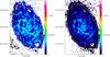Fig. 1 Dust surface density [g/cm-2] maps of M 33 at 25′′ resolution: (left) for a constant β = 2, (right) radially variable β (2−1.3) as derived in Tabatabaei et al. (2014). The ellipsed correspond to a galactocentric radius of 7 kpc.

The whole bright stellar disk of M 33 (up to a radius of ~7 kpc) was recently observed in the CO(2–1) line down to a very low noise level (Druard et al. 2014; Gratier et al. 2010a) using the IRAM 30 m telescope on Pico Veleta. The single-dish CO(2–1) data do not suffer from missing flux problems which is an essential asset to the understanding of the entire molecular phase in the galactic disk. M 33 is a chemically young galaxy with a high gas mass fraction and as such represents a different environment in which to study cloud and star formation with respect to the Milky Way. As the average metallicity is subsolar by only a factor of two and the morphology remains that of a rotating disk, M 33 represents a stepping stone towards lower metallicity and less regular objects. Measuring the link between CO and H₂ is particularly important given the evidence that the conversion of H₂ into stars becomes more efficient at lower metallicities (Gardan et al. 2007; Gratier et al. 2010a; Druard et al. 2014; Hunt et al. 2015).

With the advent of high resolution dust maps in the Herschel SPIRE and PACS, and Spitzer MIPS and IRAC bands it is possible to determine reliable dust column densities with spatial resolution close to the size of individual GMCs in M 33 (see Kramer et al. 2010; Braine et al. 2010; Xilouris et al. 2012). Under the assumption of local independence of the gas-to-dust ratio (GDR) with respect to the H₂/H i fraction, it is possible to determine the local CO intensity to H₂ column density ratio (X_CO).

A simplified global version of such an approach has been applied in Braine et al. (2010, Fig. 4). A more sophisticated method based on maximizing correlation between dust column density structure and that of the gas as derived from H i and CO through an optimal X_CO factor has recently been proposed and successfully demonstrated by Leroy et al. (2011) and Sandstrom et al. (2013).

However, these methods have biases and/or degeneracies which will be studied in Sects. 3 and 4, in particular they often do not consider a possible contribution from CO dark molecular gas. In this work, the dust, CO, and H i data covering the disk of M 33 are analyzed using existing these methods along with simulations to quantify bias and degeneracy. A new Bayesian approach is then used and tested in order to calculate the GDR and X_CO for any position but also the amount of potential CO dark gas, unseen in H i or CO. All the methods take as a basic assumption that any gas not traced by CO, or potentially optically thick H i, contains dust with similar properties as in the gas traced by CO and H i. This is common to all other studies using dust emission.

2. Data

The CO data are from the recently completed CO(2–1) survey of M 33, which now covers the bright optical disk at high sensitivity (Druard et al. 2014; Gratier et al. 2010b; Gardan et al. 2007). The H i data are from Gratier et al. (2010b). In both lines, we use the datasets produced at 25′′ resolution. The dust surface density is estimated from the Herschel observations (Kramer et al. 2010; Boquien et al. 2011; Xilouris et al. 2012), using the 100, 160, 250, and 350 micron flux densities convolved when necessary to a resolution of 25′′ (see Fig. 1). Thus, the linear spatial resolution at which this study is carried out is 100 pc.

In Fig. 1 (left panel), we show the dust surface density estimated from the SPIRE 250 and 350μm fluxes, using the ratio of these two bands to define the temperature, and assuming a dust opacity of κ = 0.4(ν/ 250 GHz)² cm² per gram of dust (Kruegel & Siebenmorgen 1994), or κ₃₅₀ = 4.7 cm² g^-1 at 350μm.

It is now clear that the dust emissivity index, traditionally designated β, is not necessarily 2 as has generally been assumed. In particular Tabatabaei et al. (2014) have shown that β is variable and lower in M 33 (β = 2−1.3 from the center to the outer disk). However, without being able to calibrate the value κ at the wavelength of interest, it is difficult to be sure of the constant (0.4 above for the dust opacity) as extrapolations have generally assumed β = 2. If the intrinsic β of the dust grains is less than 2, then using β = 2 will result in an underestimate of the temperature and thus an overestimate of the dust mass (compare the two panels of Fig. 1). In this context, a more accurate but more complex means of deriving the dust surface density has been tested. Tabatabaei et al. (2014) find a link between the galactocentric distance and β in M 33 (their Fig. 3). This β(r)is used to derive dust temperatures over the disk of M 33.

In a similar way as in Braine et al. (2010), we then take pixels with H i column density measurements and dust temperatures but no CO emission and compute the median dust cross-section (σ_dust) per H-atom: σ_dust = S_ν/ (B_ν,TN_H), where S_ν is the dust emission and B_ν,T the Planck black body emissivity for a frequency ν and a temperature T. At submillimeter wavelengths the dust emission is optically thin. This yields a cross-section per H-atom which naturally varies with radius, much like the metallicity (Magrini et al. 2009). Using σ_dust(r), we calculate the total H (i.e., cold, neutral hydrogen gas: H i + H₂) column density. The dust opacity is N_Hσ_dust = κΣ_dust = S_ν/B_ν,T(β), and the dust surface density Σ_dust = S_ν/ (B_ν,T(β)κ). For κ₃₅₀ as above, the dust surface density can be computed for all points in M 33, as shown in Fig. 1 (right panel), such that the difference with respect to Fig. 1 (left panel) is that the temperature is computed with a radially varying β. The values of β are below 2 in M 33 (Tabatabaei et al. 2014) so the temperatures are higher. Since the Planck function B_ν,T(β) increases with T, the dust surface density in Fig. 1 (right panel) is lower, particularly in the outer disk where β is lower.

In this work, we only discuss hydrogen content and do not include helium. As helium is present in both the atomic and molecular phases in equal proportion, this does not affect the calculations. As in many other works, we use the term GDR to refer to the hydrogen to dust mass ratio.

3. Dust-derived H₂ versus CO intensity

A simple approach is to take the pre-existing map of the H₂ column density based on Herschel and H i data from Braine et al. (2010) where N(H₂) is estimated from the dust and H i emission as N(H₂) = (N(H)−N(H i))/2, as in their Fig. 4.

In this case, the variables are X_CO and, potentially, a CO-dark gas column density designated ${\mathit{K}}_{\mathrm{dark}}^{\mathrm{\prime }}$. Figure 2 shows the scatter plots for a sample of three radial bins – 0 kpc < r < 1 kpc, 1 kpc < r < 2 kpc, and 4 kpc <r < 5 kpc. These radii show progressively the transition from an H₂ dominated ISM, to approximate H i–H₂ equality between radii 1 and 2 kpc, to the H i dominated outer regions.

Thick red lines show the binning of the scatter-plot in 0.5 K wide intervals. The cloud of points are fit by two lines, one assuming N(H₂) = X_CO × I_CO (light red line) and $\mathit{N}\mathrm{\left(}{\mathrm{H}}_{\mathrm{2}}\mathrm{\right)}\mathrm{=}{\mathit{X}}_{\mathrm{CO}}\mathrm{\times }{\mathit{I}}_{\mathrm{CO}}\mathrm{+}{\mathit{K}}_{\mathrm{dark}}^{\mathrm{\prime }}$ in green. As described by Dickman et al. (1986) a X_CO ratio is an average over many different clouds so it cannot be expected to characterize all clouds, or all of our data points.

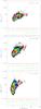Fig. 2 Fit of dust-derived N(H2) as a function of ICO for data in radial intervals between 0 and 1 kpc (top), 1−2 kpc (middle), and 4−5 kpc (bottom). No cut in intensity has been applied. The color scale indicates the density of points and the thick red histogram shows the N(H2) data averaged in bins of 0.5 K km s-1. The thin green line shows an affine fit between N(H2) and ICO; the corresponding fit results are printed in green. The thin red line is a linear fit without an offset; the corresponding fit results are printed in red. Blue cross: average value of the plotted data.

Figure 2 shows the relationship between the dust-derived H₂ column density and I_CO for three radial intervals chosen to represent the inner and outer regions, respectively H₂ dominated, slightly H i dominated (1−2 kpc), and strongly H i dominated with weak CO emission. From the inner to outer regions, the X_CO factor increases, as could be expected given that there is a metallicity gradient and a decline in CO emission (Gratier et al. 2010b) and cloud temperature (Gratier et al. 2012).

The lines without a ${\mathit{K}}_{\mathrm{dark}}^{\mathrm{\prime }}$ systematically overestimate the H₂ mass at moderate and high I_CO and both fits overestimate N(H₂) at high I_CO. There is no physical reason to expect a constant offset (${\mathit{K}}_{\mathrm{dark}}^{\mathrm{\prime }}$) but it appears that there is gas whose dust emission is detected but is not seen in CO – this could be optically thick H i, molecular gas where CO has not formed or is photodissociated, low density H₂ clouds, or unexpectedly large quantities of ionized gas.

4. Leroy-Sandstrom method

4.1. Prior discussion on the gas-to-dust ratio (GDR)

The GDR is likely well-constrained by the metallicity, at least for metallicities reasonably close to solar. The solar metallicity is about Z = 0.0142 by mass (Asplund et al. 2009, Sect. 3.1.2). Assuming the standard hydrogen-to-dust mass ratio of 100 (Draine & Li 2007, Table 3), the total gas/dust mass ratio is M(H + He + gas - phasemetals) /M(dust), assuming H and He to be negligible contributors to the dust mass. From Asplund, M(H) = 0.7154 and M(He) = 0.2703, and denoting the gas-phase-metal-fraction as Z_gas, we define the hydrogen gas-to-dust mass ratio as GDR = (0.7154 + 0.0142 Z_gas)/(0.0142(1−Z_gas)). Helium adds just under 40% to this number. For GDR = 100, the typical Galactic value, the gas-phase-metal-fraction Z_gas = 0.49 and 51% of the metals are in the dust phase. This value is reasonably robust; for a solar composition, if GDR = 100 ± 20 then 50 ± 10% of the metals are in the gas phase.

What about lower metallicity environments? Since dust condenses from the gas in AGB stellar winds (Gielen et al. 2010) and super nova remnants (Matsuura et al. 2011), one expects that when there is less dust and less metals, the gas-phase metal fraction will tend to be higher. At very low metallicities, except for very dense environments, the GDR should be higher than the relation given above due to the difficulty in forming dust grains and mantles sufficiently quickly such that evaporation or destruction processes do not reduce the dust mass (Rémy-Ruyer et al. 2014).

4.2. Method and application to M 33

Developed in Leroy et al. (2011) and later extended and applied to the HERACLES/KINGFISH data in Sandstrom et al. (2013), the idea is that the dust emission can be expressed as the sum of the emission from the atomic and molecular components, implicitly assuming that the contribution from the ionized gas is negligible. The latter assumption is likely appropriate and is also common to other studies $\begin{array}{ccc}{\mathrm{\Sigma }}_{\mathrm{gas}}& \mathrm{=}& \mathrm{GDR}\mathrm{\times }{\mathrm{\Sigma }}_{\mathrm{dust}}\\ & \mathrm{=}& {\mathit{m}}_{\mathrm{p}}\mathrm{\times }\left[\mathit{N}\mathrm{\left(}\mathrm{H}\hspace{0.17em}{i}\mathrm{\right)}\mathrm{+}\mathrm{2}{\mathit{X}}_{\mathrm{CO}}\mathrm{\times }{\mathit{I}}_{\mathrm{CO}}\right]\\ & \mathrm{=}& {\mathrm{\Sigma }}_{\mathrm{H}\hspace{0.17em}{i}}\mathrm{+}{\mathit{\alpha }}_{\mathrm{CO}}\mathrm{\times }{\mathit{I}}_{\mathrm{CO}}\end{array}$(1)where α_CO is a surface density conversion factor from I_CO to Σ_H2. Equating the right-hand terms gives us the relation equivalent to Sandstrom et al. (2013, Eq. (3)). In order to allow for some form of CO dark gas, we allow for an additional term, such that the basic equation becomes $\begin{array}{ccc}{\mathrm{\Sigma }}_{\mathrm{gas}}& \mathrm{=}& \mathrm{GDR}\mathrm{\times }{\mathrm{\Sigma }}_{\mathrm{dust}}\\ & \mathrm{=}& {\mathit{m}}_{\mathrm{p}}\mathrm{\times }\mathrm{[}\mathit{N}\mathrm{\left(}\mathrm{H}\hspace{0.17em}{i}\mathrm{\right)}\mathrm{+}\mathrm{2}{\mathit{X}}_{\mathrm{CO}}\mathrm{\times }{\mathit{I}}_{\mathrm{CO}}\mathrm{+}{{\mathit{K}}_{\mathrm{dark}}^{\mathrm{\prime }}}^{\mathrm{]}}\\ & \mathrm{=}& \end{array}$(2)The procedure is fairly simple: the α_CO – K_dark space is explored on a regularly spaced grid and, for each couple (α_CO, K_dark), the dispersion in log (GDR) over the ensemble of pixels is computed. The best fit parameters (α_CO, K_dark) are chosen as the ones that minimize the log (GDR) dispersion, similar to what was done in Leroy et al. (2011). Sandstrom et al. (2013, their appendix) later studied the influence of different methods to identify the best solution finding robust results over the different methods and settling to using a minimization of the (robust) standard deviation of the logarithm of the GDR. Our maps of M 33 cover an area of several thousand beams. This enables us to look for variations, in particular radial variations, of GDR, α_CO, and K_dark. Figure 3 shows this space for three radial intervals in M 33, with a minimum computed assuming that a single value for each of the three parameters GDR, α_CO, and K_dark is appropriate. The best fits are shown as a function of radius in Fig. 4 where the same procedure is applied to concentric elliptical rings sampling 1 kpc in radius.

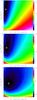Fig. 3 Scatter in log (GDR) as a function of XCO and Kdark. The color scale and solid white contours indicate the amplitude of the scatter in log (GDR) as measured by the standard deviation for varying XCO and Kdark offsets. Radii between 0 and 1 kpc (top), 1−2 kpc (middle), and 4−5 kpc (bottom). The white cross corresponds to the minimum scatter (i.e., best fit). The contours correspond to constant scatter values and give an indication of the uncertainties and degeneracies. The white lines correspond to constant GDR values of 100 (solid), 150 (dashed), 200 (dotted), 250 (dash-dotted).

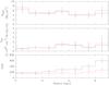Fig. 4 Average values for Kdark, XCO, and GDR derived for 1 kpc radial bins using the Leroy-Sandstrom method. The black histogram shows results derived with the variable beta (Tabatabaei et al. 2014) prescription and the red used the β = 2 to determine dust temperatures.

Figure 3 shows that a very broad region of α_CO – K_dark space yields similar quality fits but that a prior on GDR would help break this degeneracy. The radial behavior shown in Fig. 4 appears somewhat unphysical as the metallicity gradient necessarily yields an increasing GDR and would be expected to also yield X_CO increasing with radius.

If we assume that K_dark = 0, then we see from Fig. 3 (horizontal line where K_dark = 0) that the fit is clearly poorer than the best fit. The same is true for the individual radial bins. The physical interpretation of K_dark is far from straightforward. The same procedure has been applied but with a filter only accepting pixels with I_CO > 2σ. The result is essentially the same: the slope of the ellipses decreases steadily with radius, showing how difficult it is to measure X_CO in the outer regions. The radial variation of the parameters with radius is shown in Fig. 4.

The somewhat more complicated nature of the L–S method (3 parameters: α_CO, GDR and K_dark) and the broad degeneracies prompted us to explore the effect of noise on typical values (Sect. 4.4) and the recoverability of input parameters using realistic simulated data (Sect. 4.3).

4.3. Recoverability

In order to check the recoverability of the parameters, we have created simulated dust observations with known parameters α_CO, GDR and K_dark. The I_CO and I_{H i} used are the observed values for M 33 to maintain the right correlation between these two quantities. Simulated observations are created following Eq. (6). Noise is then added to each observable quantity I_CO, I_{H i} and Σ_dust.

We then create the same figures as in Sect. 4.2. The figures are not shown because they are indistinguishable in shape from those in Sect. 4.2 (Figs. 3 and 4). This is not surprising as the data are the same. However, we can add many mock runs of the noise and examine how the biases are affected by differing noise levels and intensity cuts.

Figure 5 shows the result of 200 sets of trial data based on the inner kpc. Input parameters are X_CO = 4 × 10²⁰ cm^-2/ (K km s^-1), GDR = 150 and K_dark = 5 M_⊙/ pc², indicated as red lines.

It is immediately clear that the optimization (i.e., the lowest log (GDR) dispersion in Fig. 3) favors low-valued solutions, with “optimal” values clearly below the input. Even in this high signal-to-noise (S/N) region, X_CO is underestimated by 25% as is K_dark and the GDR by half as much. The GDR is less affected because the H i column density is not modified by K_dark or X_CO but contributes close to half of the GDR.

Two variants were tested as well. Although a K_dark was present in the input parameters, we test the values obtained if it is assumed that K_dark = 0, as in Eq. (3) of Sandstrom et al. (2013). In this case, the GDR is underestimated, presumably because more dust is present (as a K_dark was injected) than what is seen in H i or CO. Near the center, (Fig. 5) X_CO is underestimated (see middle row) but at larger radii the situation is different (cf. next paragraph). If metallicity measurements are reliable, then the GDR is quite constrained (Sect. 4.1). The top row shows the values for X_CO and K_dark if the true GDR is injected. If a prior on GDR is injected, then we approximately recover X_CO and K_dark. The dispersion in the histograms is rather small, showing that the results do not depend on the number of realizations.

In the H i dominated outer regions, Fig. 6 shows the same biases as before except that X_CO is overestimated when K_dark is forced to zero. The prior on GDR again helps recover the input values with reasonable fidelity. There is only weak CO emission at these radii so the constraint on X_CO is weak. We therefore made a test excluding values where I_co< 2σ. The differences with respect to the input parameters are somewhat less severe (compare Figs. 6 and 7). For the inner kpc, excluding values below 2σ makes no difference because virtually all of the values exceed the threshold.

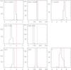Fig. 5 Histogram of recovered values for the generative model including noise in all three observables XCO, GDR, and Kdark. Bottom row: recovering the 3 parameters. Middle row: recovering only αCOand GDR even though Kdark is present in the data. Top row: same as bottom row but imposing the correct value of GDR. This figure is for the central kpc of M 33. Input values are in red.

Fig. 6 Same as Fig. 5 but for 4 kpc <R< 5 kpc.

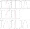Fig. 7 Same as Fig. 6 but only considering pixels where ICO > 2σ. A similar cut for the central radii would show little effect as the CO signal there is strong.

4.4. Noise effects

In order to evaluate the behavior of the Leroy-Sandstrom (L-S) method in the presence of noise, we took typical values of the CO intensity, the H i column, and noise for both, in order to test how the method was affected by noise. We also allow for the presence of CO dark gas, where dark means gas not observed in CO or H i but detected via the emission of the associated dust. Thus, we start with a single value for each of I_CO, N(H i) (optically thin assumption), and K_dark (dark gas, assumed constant). Assuming a X_CO conversion factor, we calculate the gas column density (N(H) = 2 × X_CO × I_CO + N(H i) + K_dark) which we divide by an assumed gas-to-dust ratio (GDR) to obtain a dust surface density Σ_dust, similar to what is estimated from analyses of Herschel photometric data (Kramer et al. 2010; Xilouris et al. 2012; Tabatabaei et al. 2014). We then assume a noise level in the same units for each of these quantities and generate 1000 samples (value + Gaussian noise) of each of I_CO, N(H i), K_dark, and Σ_dust. Σ_dust after addition of noise is then converted back into a gas surface density using the same GDR. The final step is to test a grid of X_CO and K_dark values, minimizing the sum of $\mathrm{(}{\mathrm{\Sigma }}_{\mathrm{dust}}\mathrm{GDR}\mathrm{-}{\mathit{\alpha }}_{\mathrm{CO}}{\mathit{I}}_{\mathrm{CO}}\mathrm{-}{\mathrm{\Sigma }}_{\mathrm{H}\hspace{0.17em}{i}}\mathrm{-}{\mathit{K}}_{\mathrm{dark}}\mathrm{)}2$(3)where the quantities are after addition of noise and the sum is over the 1000 samples.

The fiducial model has I_CO = 1 ± 0.25 K km s^-1, N(H i)=8 ± 1 × 10²⁰ cm^-2, and K_dark = 1 ± 0.25 × 10²⁰ cm^-2 and we assume the uncertainty in the dust surface density is 25%. We inject X_CO = 4 × 10²⁰ cm^-2/ (K km s^-1) in order to calculate Σ_gas – this, along with K_dark, is what we try to get out of the simulations. The GDR is transparent in that it is used to convert Σ_gas into Σ_dust but then back into Σ_gas after addition of noise so it disappears.

Figure 8 shows the typical degeneracy between the X_CO and K_dark parameters. The color scale shows the quality of the fit (the lower the better) and contours show the acceptable regions. The black dotted lines indicate the average gas-to-dust ratio for the pixel (i.e., averaged over the 1000 samples for the (I_CO,K_dark) combination). The dotted lines indicate, from left to right, GDRs of 100, 150, 200, and 250. For this example, with I_CO = 0.5 ± 0.25 K km s^-1, the apparently optimal fit is quite far from the input parameters. These values are quite typical of a large number of the pixels in M 33.

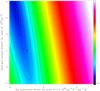Fig. 8 Quality of fit for model with ICO = 1 ± 0.25 K km s-1, N(H i) = 8 ± 1 × 1020 cm-2, and Kdark = 1 ± 0.25 × 1020 cm-2, assuming that the uncertainty in the dust surface density is 25%. Dotted lines represent, from left to right, constant GDR values of 100, 150, 200, 250. The star at XCO = 4 × 1020 cm-2/ (K km s-1) is the input value but the best fit is far from that.

Figures 9a−f show how the retrieved values of X_CO and K_dark vary with the CO intensity (before adding noise) and the noise level of the CO observations. The first two figures show the results for N(H i) = 8 ± 1 × 10²⁰ cm^-2 and a 25% uncertainty in the dust surface density. The second set of figures shows how the recovered X_CO and K_dark values depend on the CO intensity and uncertainty in the case where N(H i) = 4 ± 1 × 10²⁰ cm^-2. In the third set, N(H i) = 8 ± 1 × 10²⁰ cm^-2 but the uncertainty in the dust (and thus gas) surface density has been reduced to 10%.

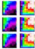Fig. 9 Optimal retrieved values of XCO (left column) and K (right column) as a function of the CO intensity (before adding noise) and the noise level of the CO observations. Top figures: fiducial model. Middle row: fiducial except H i column density reduced to 4 × 1020 cm-2. Bottom: fiducial except dust uncertainties reduced to 10%.

The result is striking: in all cases, the X_CO conversion factor and the K_dark surface density are well recovered for the high CO intensities and small errors but where the intensity or the S/N is lower the recovered X_CO decreases systematically and the amount of dark gas increases rapidly. A general tendency is seen towards high K_dark and low X_CO as the S/N decreases, similar to Fig. 8.

5. Bayesian method

5.1. Principles

This method enables us to take into account the uncertainties in all of the observed quantities and recover the best estimates of the GDR, X_CO, and K_dark values. This is done in the Bayesian framework of errors in variables.

The generative model is defined as: $\begin{array}{ccc}& & \\ & & \\ & & \\ & & \end{array}$The above notation means that the quantity ${\mathit{I}}_{\mathrm{H}\hspace{0.17em}{i}\mathit{,i}}^{\mathrm{obs}}$ observed at pixel i has a Gaussian distribution centered on the true ${\mathit{I}}_{\mathrm{H}\hspace{0.17em}{i}\mathit{,i}}^{\mathrm{true}}$ integrated intensity with a dispersion equal to the observational uncertainty σ_{H i,i}. Same for the CO in Eq. (5). The third line states that the true dust surface density Σ_dust,i is a function of the true I_{H i,i} and I_CO,i and the three model parameters α_CO, GDR and K_dark. We assume that the H i emission is optically thin such that X_{H i} = 1.823 × 10¹⁸ cm^-2/ (K km s^-1) which converted into units of solar masses per square pc gives α_{H i} = 0.0146 M_⊙/ pc²/ ( K km s^-1). The fourth equation states that the observed dust surface density (left) has a gaussian distribution centered on the true Σ_dust,i with dispersion of σ_Σdust. We note that the only equality is for the true quantities, not the observations. This method provides an estimate for the true values of Σ_dust, I_CO, and I_{H i}, as well as the parameters α_CO, GDR, K_dark.

Because the observations are independent, we can express the likelihood of the parameters knowing the full dataset as the product of the likelihoods of the parameters knowing each individual datapoint. For N observations, $\begin{array}{ccc}& & \mathit{L}\mathrm{\left(}\mathit{a,b,c,}\mathrm{\right\{}{\mathit{I}}_{\mathrm{CO}\mathit{,i}}^{\mathrm{true}}\mathrm{\left\}}\mathit{,}\mathrm{\right\{}{\mathit{I}}_{\mathrm{H}\hspace{0.17em}{i}\mathit{,i}}^{\mathrm{true}}\mathrm{\left\}}\mathit{,}{\mathit{\sigma }}_{\mathrm{dust}}\mathrm{\right|}\mathit{D}\mathrm{)}\mathrm{=}\\ & & \mathit{p}\mathrm{\left(}\mathit{D}\mathrm{\right|}\mathit{a,b,c,}\mathrm{\left\{}{\mathit{I}}_{\mathrm{CO}\mathit{,i}}^{\mathrm{true}}\mathrm{\right\}}\mathit{,}\mathrm{\left\{}{\mathit{I}}_{\mathrm{H}\hspace{0.17em}{i}\mathit{,i}}^{\mathrm{true}}\mathrm{\right\}}\mathit{,}{\mathit{\sigma }}_{\mathrm{dust}}\mathrm{)}\mathrm{=}\frac{\mathrm{(}\mathrm{2}\mathit{\pi }{\mathrm{)}}^{\mathit{N}}}{{\mathrm{􏽑}}_{\mathit{i}\mathrm{=}\mathrm{1}}^{\mathit{N}}\sqrt{{\mathit{\sigma }}_{{\mathit{I}}_{\mathrm{CO}}\mathit{,i}}^{\mathrm{2}}{\mathit{\sigma }}_{{\mathit{I}}_{\mathrm{H}\hspace{0.17em}{i}}\mathit{,i}}^{\mathrm{2}}{\mathit{\sigma }}_{{\mathrm{\Sigma }}_{\mathrm{dust}}}^{\mathrm{2}}}}\\ & & \mathrm{\times }\underset{\mathit{i}\mathrm{=}\mathrm{1}}{\overset{\mathit{N}}{\mathrm{􏽙}}}\exp \left[\mathrm{-}\frac{\mathrm{(}{\mathit{I}}_{\mathrm{CO}\mathit{,i}}^{\mathrm{obs}}\mathrm{-}{\mathit{I}}_{\mathrm{CO}\mathit{,i}}^{\mathrm{true}}{\mathrm{)}}^{\mathrm{2}}}{\mathrm{2}{\mathit{\sigma }}_{{\mathit{I}}_{\mathrm{CO}}\mathit{,i}}^{\mathrm{2}}}\right]\\ & & \mathrm{\times }\underset{\mathit{i}\mathrm{=}\mathrm{1}}{\overset{\mathit{N}}{\mathrm{􏽙}}}\exp \left[\mathrm{-}\frac{\mathrm{(}{\mathit{I}}_{\mathrm{H}\hspace{0.17em}{i}\mathit{,i}}^{\mathrm{obs}}\mathrm{-}{\mathit{I}}_{\mathrm{H}\hspace{0.17em}{i}\mathit{,i}}^{\mathrm{true}}{\mathrm{)}}^{\mathrm{2}}}{\mathrm{2}{\mathit{\sigma }}_{{\mathit{I}}_{\mathrm{H}\hspace{0.17em}{i}}\mathit{,i}}^{\mathrm{2}}}\right]\\ & & \end{array}$(8)where D is the observed dataset $\mathrm{\left\{}\mathrm{\right\{}{\mathit{I}}_{\mathrm{CO}\mathit{,i}}^{\mathrm{obs}}\mathrm{\left\}}\mathit{,}\mathrm{\right\{}{\mathit{I}}_{\mathrm{H}\hspace{0.17em}{i}\mathit{,i}}^{\mathrm{obs}}\mathrm{\left\}}\mathit{,}\mathrm{\right\{}{\mathrm{\Sigma }}_{\mathrm{dust}\mathit{,}\mathrm{i}}^{\mathrm{obs}}\mathrm{\left\}}\mathrm{\right\}}$, 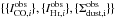a = α_{H i}/ GDR, b = α_CO/ GDR, c = K_dark/ GDR. The likelihood is thus the probablility of having an observed set of $\mathrm{\left\{}\mathrm{\right\{}{\mathit{I}}_{\mathrm{CO}\mathit{,i}}^{\mathrm{obs}}\mathrm{\left\}}\mathit{,}\mathrm{\right\{}{\mathit{I}}_{\mathrm{H}\hspace{0.17em}{i}\mathit{,i}}^{\mathrm{obs}}\mathrm{\left\}}\mathit{,}\mathrm{\right\{}{\mathrm{\Sigma }}_{\mathrm{dust}\mathit{,}\mathrm{i}}^{\mathrm{obs}}\mathrm{\left\}}\mathrm{\right\}}$ (i.e., the observed map of Σ_dust, I_CO and I_{H i}) given a set of values for α_{H i}/ GDR, α_CO/ GDR, K_dark/ GDR, {${\mathit{I}}_{\mathrm{CO}\mathit{,i}}^{\mathrm{true}}$}, $\mathrm{\left\{}{\mathit{I}}_{\mathrm{H}\hspace{0.17em}{i}\mathit{,i}}^{\mathrm{true}}\mathrm{\right\}}$, and σ_Σdust. We know the uncertainty in the I_CO and I_{H i} observations (σ_{IH i},σ_ICO) and the values are input to the calculation. On the other hand, we do not have a good estimate of the uncertainty in the dust surface density σ_Σdust so this is left as a free parameter and becomes an output of the calculation. This σ_Σdust will also parameterize Gaussian scatter around the true relationship so σ_Σdust may be larger than the measurement error, but accounts for additional scatter in the data (Hogg et al. 2010).

Thus, there are 4 + 2N parameters (α_{H i}/ GDR, α_CO/ GDR, K_dark/ GDR, σ_Σdust and the ${\mathit{I}}_{\mathrm{CO}\mathit{,i}}^{\mathrm{true}}$ and ${\mathit{I}}_{\mathrm{H}\hspace{0.17em}{i}\mathit{,i}}^{\mathrm{true}}$ for each of the N pixels) to the model and a total of 3N observations (${\mathrm{\Sigma }}_{\mathrm{dust}\mathit{,}\mathrm{i}}^{\mathrm{obs}}\mathit{,}{\mathit{I}}_{\mathrm{CO}\mathit{,i}}^{\mathrm{obs}}\mathit{,}{\mathit{I}}_{\mathrm{H}\hspace{0.17em}{i}\mathit{,i}}^{\mathrm{obs}}$ for each pixel).

Since we are interested in the distribution of the parameters and the likelihood is a probability distribution for the observations, we use the Bayes formula to convert from one to the other. $\begin{array}{ccc}& & \mathit{p}\mathrm{\left(}\mathit{a,b,c,}\mathrm{\right\{}{\mathit{I}}_{\mathrm{CO}\mathit{,i}}^{\mathrm{true}}\mathrm{\left\}}\mathit{,}\mathrm{\right\{}{\mathit{I}}_{\mathrm{H}\hspace{0.17em}{i}\mathit{,i}}^{\mathrm{true}}\mathrm{\left\}}\mathit{,}{\mathit{\sigma }}_{{\mathrm{\Sigma }}_{\mathrm{dust}}}\mathrm{\right|}\mathit{D}\mathrm{)}\mathrm{\propto }\\ & & \mathit{p}\mathrm{\left(}\mathit{a,b,c,}\mathrm{\right\{}{\mathit{I}}_{\mathrm{CO}\mathit{,i}}^{\mathrm{true}}\mathrm{\left\}}\mathit{,}\mathrm{\right\{}{\mathit{I}}_{\mathrm{H}\hspace{0.17em}{i}\mathit{,i}}^{\mathrm{true}}\mathrm{\left\}}\mathit{,}{\mathit{\sigma }}_{{\mathrm{\Sigma }}_{\mathrm{dust}}}\mathrm{\right)}\\ & & \end{array}$(9)The left hand side of Eq. (9) is the posterior distribution – the distribution function of the parameters given the observations. The first term on the right is the prior distribution of the parameters. In our case, very little information is injected because only unreasonable values are not tested. GDR is varied either uniformly from 0 to 500 or uniformly from 0 to 50 000, the first case enables to check the influence of using a physically justifies prior, namely that the GDR values cannot be higher than 500. α_CO is varied from 0 to 30 times M_⊙/ pc²/ K km s^-1 and K_dark from −10 to 30 M_⊙/ pc². The ${\mathit{I}}_{\mathrm{H}\hspace{0.17em}{i}\mathit{,i}}^{\mathrm{true}}$ and ${\mathit{I}}_{\mathrm{CO}\mathit{,i}}^{\mathrm{true}}$ parameters are varied between the minimum and the maximum of the observations. The last term is the probability defined above. The posterior distribution is explored using an Monte Carlo Markov Chain (MCMC) code, specifically the EMCEE Python implementation (Foreman-Mackey et al. 2013) of Affine Invariant Ensemble Sampler described in Goodman & Weare (2010).

The priors can be summarized as: 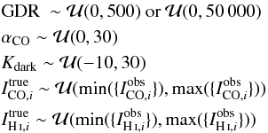$\begin{array}{ccc}& & \mathrm{GDR}\mathrm{~}\mathrm{𝒰}\mathrm{\left(}\mathrm{0}\mathit{,}\mathrm{500}\mathrm{\right)}\mathrm{or}\mathrm{𝒰}\mathrm{\left(}\mathrm{0}\mathit{,}\mathrm{50}\hspace{0.17em}\mathrm{000}\mathrm{\right)}\\ & & {\mathit{\alpha }}_{\mathrm{CO}}\mathrm{~}\mathrm{𝒰}\mathrm{\left(}\mathrm{0}\mathit{,}\mathrm{30}\mathrm{\right)}\\ & & {\mathit{K}}_{\mathrm{dark}}\mathrm{~}\mathrm{𝒰}\mathrm{(}\mathrm{-}\mathrm{10}\mathit{,}\mathrm{30}\mathrm{)}\\ & & {\mathit{I}}_{\mathrm{CO}\mathit{,i}}^{\mathrm{true}}\mathrm{~}\mathrm{𝒰}\mathrm{\left(}\min \mathrm{\right(}\mathrm{\left\{}{\mathit{I}}_{\mathrm{CO}\mathit{,i}}^{\mathrm{obs}}\mathrm{\right\}}\mathrm{\left)}\mathit{,}\max \mathrm{\right(}\mathrm{\left\{}{\mathit{I}}_{\mathrm{CO}\mathit{,i}}^{\mathrm{obs}}\mathrm{\right\}}\mathrm{\left)}\mathrm{\right)}\\ & & {\mathit{I}}_{\mathrm{H}\hspace{0.17em}{i}\mathit{,i}}^{\mathrm{true}}\mathrm{~}\mathrm{𝒰}\mathrm{\left(}\min \mathrm{\right(}\mathrm{\left\{}{\mathit{I}}_{\mathrm{H}\hspace{0.17em}{i}\mathit{,i}}^{\mathrm{obs}}\mathrm{\right\}}\mathrm{\left)}\mathit{,}\max \mathrm{\right(}\mathrm{\left\{}{\mathit{I}}_{\mathrm{H}\hspace{0.17em}{i}\mathit{,i}}^{\mathrm{obs}}\mathrm{\right\}}\mathrm{\left)}\mathrm{\right)}\end{array}$(10)where stands for a uniform distribution between values x_min and x_max.

5.2. Validation of the Bayesian method

To test the Bayesian method, we simulated a dataset using α_CO = 2 × 3.2 M_⊙/ pc²/ K km s^-1 (twice the galactic value), GDR = 150, K_dark = 10 M_⊙/ pc² and σ_Σdust = 0.01 M_⊙/ pc². Since we need to input “true” values of I_CO and I_{H i} in order to see if we can recover the parameters we inject the observed values of I_CO and I_{H i}. These values are then used to create the “true” dust map as per Eq. (6). Since the method starts with observations, we take the simulated observed values to be the real observed values plus noise. Thus, the calculation uses somewhat noisier values than the real data. The tests use datapoints (I_{H i},I_CO) characteristic of the inner disk of M 33. Noise is also added to the “true” dust surface density map (created via Eq. (6)).

This model dataset is then used as input into the Bayesian method described in Sect. 5.1. Figure 10 shows the number density of points in the six planes mixing the four parameters α_CO, GDR, K_dark, and σ_dust in grayscale. The orientation of the contours illustrates any degeneracies in the relationship between the parameters. The input parameters to the simulation are shown as solid blue lines. The 4 histograms show the entire set of values for each parameter and the dashed lines show the median and the ± 1σ and ± 2σ. The results contain no obvious bias and are very close to the input parameters. Furthermore, the confidence intervals (± 1σ and ± 2σ) are determined in a self-consistent way.

Figure 10 is the result of a simulation of the inner kpc of M 33. In the outer parts, the CO emission is very weak and the gas (and thus dust) surface density is dominated by the H i. The Bayesian method as proposed here is not always able to measure the X_CO factor where there is little CO emission but an upper limit comes out naturally. On the other hand, GDR can be measured because H i is present in many pixels.

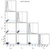Fig. 10 Test of the Bayesian method. The input values for the simulation are shown as blue lines and these correspond rather well to the peaks of probability distributions determined by the method. The dashed lines indicate the median and ± 1σ and ± 2σ intervals.

5.3. Application to M 33

M 33 was divided into 324 macropixels measuring 500 pc × 500 pc, each containing 225 independent pixels of H i, CO, and dust data. This size is large enough that the parameters are well-defined but small enough not to be affected by large-scale gradients. From the results for the macropixels, it is possible to estimate the radial variation of each parameter. The large number of pixels and macropixels results in an extremely high computation time – about six months CPU using a machine with 12 processors and 128 Gb of memory.

Nearly all (99%) of this time is taken up by the “error in variables” approach (using the full model consisting of all four Eqs. (4) to (7)). Thus, given the prohibitive CPU time, we tested the Bayesian estimation without the error in variables (using a restricted model consisting of only Eqs. (6) and (7)), which runs in a day so we can test different hypotheses. The cases we would like to test are: using the two different dust maps, with different cuts in CO intensity, and with or without limits on the value that GDR can take.

The “error in variables” approach produces slightly lower uncertainties but essentially the same values for the parameters GDR, X_CO, and K_dark. This can be seen in Fig. 11 which shows the values of K_dark, α_CO, and GDR for the error-in-variables and the rapid versions. In these simulations, the dust surface density for the variable-β was used, only pixels with CO intensities above 3σ were included, and GDR was allowed to take values between 0 and 500 (5 times the Galactic value).

Therefore, we use the rapid (1 CPU-day) computations in the following.

Even with the Bayesian approach, some degeneracy is present. In Fig. 12 (result) and 13 (radial), we show the results for variable-β dust with a 3σ CO cut but without placing a limit on GDR. Both K_dark (upper panel) and GDR (lower panel) diverge at large radii, where the CO becomes less of a constraint. This is due to some pixels reaching arbitrarily high GDR values (thousands). If the CO cut is reduced to 0σ, then K_dark and GDR diverge at lower radii. The hydrogen mass to dust mass ratio in the Milky Way is about 100, close to 140 if He is included. We thus decided to limit GDR, not allowing it to go above 500 (close to 700 if He is included). Presumably this is well above any true GDR value for a half-solar metallicity galaxy. The X_CO factor is not very affected by the divergence of K_dark and GDR although it is difficult to be confident of its value where there is little CO.

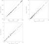Fig. 11 Comparison of rapid and full errors-in-variables Bayesian simulations. The solid line represents the equality of the two quantities and the dashed (resp. dotted) lines are constant ratios of 0.25 (resp. 0.5).

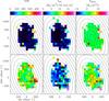Fig. 12 Results of Bayesian analysis with a 3σ cut in CO and no cap on GDR. Top row is Kdark (left) and uncertainty in Kdark (right), both with the color scale to the right and in units of M⊙/ pc2. The second row is XCO (left) and uncertainty in XCO (right), both with the color scale to the right and in units of M⊙/ pc2 per K km s-1. Bottom row is GDR (left) and uncertainty in GDR (right), both with the color scale to the right. As with the other figures, we have adopted the variable-beta dust surface density shown in Fig. 2.

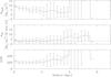Fig. 13 Radial variation of Kdark, αCO, and GDR for the simulation with a cut at 3σ for the CO but no cap on GDR. The value is computed using the maps in Fig. 12 and weighting each macropixel according to is area within a given radial annulus. The error bars indicate the dispersion within this ring. A divergence of Kdark and GDR can be seen in the outer part.

Figure 14 shows the maps of the number of measurements used for each of the macropixels for the 0σ and 3σ CO cuts.

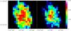Fig. 14 Maps of the number of pixels in each macropixel for the 0σ (left) and 3σ (right) CO cuts.

Figure 15 is similar to Fig. 4 in that it shows the influence of the choice of the dust emissivity index β on the derived parameters. For the Bayesian method, as for the LS method, the results are consistent for α_CO and K_dark but differ for GDR with smaller values found for the β = 2 dust maps. This is expected as the β = 2 maps has hight dust surface densities, particularly at higher radii.

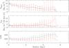Fig. 15 Average values for Kdark, XCO, and GDR derived for 0.5 kpc radial bins using the Bayesian method. The black histogram shows results derived with the variable beta of Tabatabaei et al. (2014) and the red uses the standard β = 2 to determine dust temperatures.

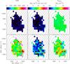Fig. 16 As for Fig. 12 but with a 500 cap on GDR. The differences can be seen in the outer parts where some of the high GDR pixels from Fig. 12 which were white because they had values over 500.

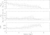Fig. 17 Radial variation of Kdark, αCO, and GDR for the simulation with a cut at 3σ for the CO and GDR capped at 500. The value is computed using the maps in Fig. 16 and weighting each macropixel according to is area within a given radial annulus. The error bars indicate the dispersion within this ring.

Fig. 18 Results of Bayesian analysis with a 0σ cut in CO and GDR limited to 500. Top row is Kdark (left) and uncertainty in Kdark (right), both with the color scale to the right and in units of M⊙/ pc2. The second row is XCO (left) and uncertainty in XCO (right), both with the color scale to the right and in units of M⊙/ pc2 per K km s-1. Bottom row is GDR (left) and uncertainty in GDR (right), both with the color scale to the right. As with the other figures, we have adopted the variable-beta dust surface density shown in Fig. 2.

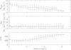Fig. 19 Radial variation of Kdark , αCO, and GDR for the simulation with a cut at 0σ for the CO and GDR capped at 500. The value is computed using the maps in Fig. 18 and weighting each macropixel according to is area within a given radial annulus. The error bars indicate the dispersion within this ring. The comparison with the preceding figures shows that the cap on GDR is critical to avoid diverging values of GDR and Kdark.

Figures 16 (result) and 17 (radial) show the same as Figs. 12 and 13 but when GDR cannot take values above 500. This essentially avoids finding an optimal result at extremely high GDR and K_dark. Where the CO is present in a significant number of pixels (Fig. 14), the limitation (of GDR) is unnecessary but when the equation really only equates GDR and K_dark then they are highly degenerate.

Figures 18 (result) and 19 (radial) show the radial variation of K_dark, X_CO, and GDR for the 0σ and 3σ CO cuts. The similarity shows that when GDR is not allowed to take unphysical values, the CO cut is not critical.

The values of GDR we find in the outer regions using the variable-β approach are actually consistent with the GDR found by Gordon et al. (2014) in the Large Magellanic Cloud. The LMC is a useful comparison as it is only slightly smaller, less massive, and less metallic than M 33 but the LMC is much more irregular.

Several interesting features are present. First of all, even though GDR increases with radius, K_dark decreases. This shows that the increase in K_dark seen without the limit on GDR was only due to the divergent pixels. The X_CO shows no clear radial trend. This is probably unlike large spirals like our own, where a number of works have suggested the X_CO increases with radius (Sodroski et al. 1995; Braine et al. 1997), with a particularly low value in the central regions. However, large spirals also show systematic decreases in the CO(2–1)/CO(1–0) ratio whereas M 33 does not (Druard et al. 2014). The value of X_CO is only 10% greater than the Galactic value, indicated by a horizontal line in Figs. 13, 17, and 19. This may appear surprising as the X_CO factor is expected to increase as the metallicity decreases.

The X_CO factor derived here is not directly comparable to the values for the Galactic X_CO derived using dust and/or gamma-ray observations because these calculations did not allow for dark gas and thus attributed all gas (including any CO dark gas) not identified as H i to H₂ in order to calculate X_CO. In order to calculate a comparable ratio, we can add the CO dark gas to the H₂ column computed as I_CO × X_CO. While typically modeled as a constant, K_dark is not physically expected to be constant as (a) H i is expected to be optically thick only over very small areas and (b) GMC edges, where H is molecular but CO photodissociated, are only expected to be associated with GMCs, which occupy a very small fraction of the disk (Druard et al. 2014). Thus, we can either take the value of K_dark derived for the CO detected (0 or 3σ) positions in the macropixel as representative of all positions, or we can assume that the value of K_dark derived for the CO detected pixels are only valid for those pixels and assume zero elsewhere. In this way, we may be able to place upper and lower limits to the total X_CO values in M 33, including dark gas.

We thus consider Fig. 10 from Druard et al. (2014) and uncorrect for inclination, uncorrect for He, and rescale to a X_CO value of 1.1 Galactic – this is equivalent to dividing their values by 1.24. To this, we can add the K_dark as computed either in (a) or (b) above.

Expressing the CO-emitting H₂ and K_dark as surface densities in Fig. 20, it is interesting to note that they are very comparable for a X_CO = 1.1X_gal where X_gal is taken to be 2 × 10²⁰ cm^-2/ K km s^-1. If we assume that the dark gas is actually molecular gas, then the two columns should be added in order to compare with the Galactic X_CO factors based on dust or gamma-rays. Depending on whether K_dark is assumed to be present everywhere at the level derived from the positions respecting the CO threshold or only for those positions, the total X_CO (dark H₂ + CO-emitting H₂ divided by I_CO) is about twice Galactic with very little radial variation (except for the case where the only pixels with K_dark are those above 3σ in CO). The uncertainties increase dramatically beyond 4.5 kpc so we have not been able to derive constraints for the very outer disk of M 33.

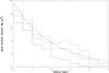Fig. 20 H2 surface density derived from CO and Kdark derived from the Bayesian analysis. The continuous curve shows ΣH2 based on Fig. 10 of Druard et al. (2014) corrected to a XCO factor of 1.1 Galactic and uncorrected for inclination and helium content. The histograms show the CO dark gas surface density. The solid histogram shows Kdark as derived assuming that all positions have the same dark column as the positions where CO is detected above the threshold. The dashed and dotted histograms represent Kdark assuming that the dark column only is present where CO is detected above the 0σ and 3σ thresholds respectively.

Although we initially expected K_dark to increase (at least with respect to CO) with galactocentric distance as in Pineda et al. (2013, Fig. 15), is not surprising the K_dark decreases with radius because the UV field decreases much more quickly than the metallicity. As for the expected increase of X_CO with galactocentric radius as is observed in large spirals (Sodroski et al. 1995; Braine et al. 1997), it is not seen in M 33. This was initially a surprise but the constant CO line ratios (2–1/1–0 and 3–2/1–0) support this. In large spirals we see clear decreases in these line ratios (and increases in X_CO), but this is not the case in M 33. We did not initially expect K_dark to follow the CO column density variation – that came out of the analysis. However, it is natural if the CO dark gas is in the outskirts of GMCs. This implies that there is no large population of diffuse H₂ clouds (unrelated to GMCs) without CO emission.

Our findings are in apparent disagreement with Pineda et al. (2013). However, Pineda et al. (2013) computed H column densities assuming a constant ratio. Introducing a radially decreasing would at least reduce the difference in our findings. Our findings are in agreement with Mookerjea et al. (2016) who find more CO dark gas near the center than in the BCLMP302 region, although it is very difficult to generalize from a small number of regions. While we describe K_dark as decreasing with radius, that is only true in an absolute sense, just like many other quantities decrease with radius (galactocentric distance). Assuming that K_dark is not attributable to optically thick H i, a roughly constant mass fraction of molecular material is CO dark, independent of radius. This is in agreement with the findings of Wolfire et al. (2010) where they model the dark gas as the region surrounding molecular clouds where the CO is photo-dissociated but not the H₂. This is in excellent agreement with our observations.

It is worth noting that there is no reason to think that the amount of gas not traced by CO or H i should be constant. Figure 21 shows the dust surface density as a function of the H i column density for 3 macropixels near the center and 3 macropixels between 4 and 5 kpc from the center. Examining the central pixels, it is immediately apparent that the intercept (K_dark), varies significantly from one pixel to another, even for neighboring regions. Comparing with the lower panel, we see that K_dark tends to be lower in the outskirts although for example, for the brown dots the distribution is rather flat (moderate K_dark, infinite GDR) at least when only the H i is plotted. Assuming no CO is present at low H i column density, it is also immediately apparent that there is more dust per unit gas near the center, which is the equivalent of a radially increasing GDR. The low (high) GDR is a factor common to all three pixels at small (large) radii.

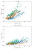Fig. 21 Top: link between H i column density and dust surface density for 3 macro-pixels near the center of M 33. Each color represents the pixel values of N(H i) and Σdust for a single macro-pixel. Bottom: same as above but for 3 macro-pixels between 4 and 5 kpc from the center.

6. Conclusions

In order to investigate how GDR, X_CO, and K_dark vary in M 33, the first step was to take a published estimate of the gas column density N(H)_dust based on the Herschel dust observations and plot N(H)_dust−N(H i) versus I_CO. The systematically positive intercept (Fig. 2) suggests that there is low-column density gas traced by dust but not CO or H i, which we refer to as K_dark (Tielens & Hollenbach 1985; Planck Collaboration XIX 2011).

The next step is to construct a map of the dust surface density. Two methods were used – the classical β = 2 dust emissivity (Fig. 1, left panel) and the variable-β (same figure, right panel) developed by Tabatabaei et al. (2014). We adopt the second method because in other subsolar metallicity galaxies (Galliano et al. 2011) the classical approach yields too large a dust mass, presumably due to a change in grain properties with respect to Milky Way dust. Using β = 2 for M 33 also yields a very high dust mass and Tabatabaei et al. (2014) show that β = 2 is a poor approximation for M 33.

We then look for optimal values of GDR, X_CO, and K_dark to relate the dust surface density to the H i and CO intensities. Except where the S/N is high, major degeneracies are present between these parameters (Fig. 3) such that they all increase (or decrease) simultaneously with similar scatter in log (GDR).

Using simulated data with noise, a similar effect is seen in that the deduced solutions generally have lower GDR, X_CO, and K_dark than the input values (Figs. 5–7). Setting GDR to the correct (input) value yields reasonably accurate results. Solving only for GDR and X_CO, implicitly assuming K_dark = 0 when the input value was K_dark = 5M_⊙/ pc², yields results for GDR and X_CO that strongly depend on the amount of CO with respect to H i. The degeneracies are illustrated by Figs. 8 and 9.

An extremely computation-intensive simulation using the Bayesian errors-in-variables approach was used to obtain “true” values of the parameters. Fortunately, a very similar result can be obtained using the Bayesian formalism but without the errors-in-variables approach, as shown from the comparison in Fig. 11. The main difference is the slightly lower uncertainty with the errors-in-variables approach. The degeneracies present using the other methods are (almost) no longer an issue (Fig. 22).

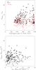Fig. 22 Search for degeneracies between the GDR, XCO, and Kdark in the Bayesian approach. Top panel: XCO (αCO) and Kdark as a function of GDR. Bottom panel: link (or absence) between XCO (αco) and Kdark. Each point represents a pixel in the maps shown in Fig. 16.

There is a radial increase in GDR from ~200 near the center to nearly 400 in the outer disk. The X_CO ratio remains constant with galactocentric distance, as does the CO(2−1)/CO(1−0) line ratio (Druard et al. 2014) and CO(3−2)/CO(2−1) line ratio (in prep.), unlike what is observed in large spirals. The surface density of dark gas, K_dark, decreases from the center (10M_⊙/ pc²) to the outer parts (roughly zero) in the same way as the CO emission such that the dark gas represents close to half of the H₂ assuming that the dark gas is in fact H₂. As a result, the ratio of all H₂ (dark gas plus the H₂ traced directly by CO), is about twice the local value of 2 × 10²⁰ cm^-2/ K km s^-1.

Some traces of the degeneracies between K_dark and GDR are still present in that some macropixels with little CO find optimal values that are physically unrealistic (typically GDR ~ 5000 with a corresponding divergence of K_dark). Limiting the GDR to values less than 500 (5 times the Milky Way value) avoids the problem.

Overall, our results argue for a fairly high GDR in M 33 (GDR ≥ 200), a radially decreasing K_dark roughly proportional to the amount of CO emission, and a fairly constant X_CO conversion both of the H₂ directly traced by CO and the total H₂ content including the dark gas (whose radial distribution is similar to that of the CO).

The results presented here on the link between CO and total molecular gas mass (and/or any optically thick H i) confirm the earlier estimates of the H₂ mass of M 33. As a result, either the H₂ is converted into stars more quickly than in large spirals or the star-formation rate is overestimated due to for example a change in IMF in this environment.

Acknowledgments

P.G. thanks ERC starting grant (3DICE, grant agreement 336474) for funding during this work. P.G.’s current postdoctoral position is funded by INSU/CNRS.

References

All Tables

All Figures

	Fig. 1 Dust surface density [g/cm-2] maps of M 33 at 25′′ resolution: (left) for a constant β = 2, (right) radially variable β (2−1.3) as derived in Tabatabaei et al. (2014). The ellipsed correspond to a galactocentric radius of 7 kpc.
In the text

Fig. 2 Fit of dust-derived N(H2) as a function of ICO for data in radial intervals between 0 and 1 kpc (top), 1−2 kpc (middle), and 4−5 kpc (bottom). No cut in intensity has been applied. The color scale indicates the density of points and the thick red histogram shows the N(H2) data averaged in bins of 0.5 K km s-1. The thin green line shows an affine fit between N(H2) and ICO; the corresponding fit results are printed in green. The thin red line is a linear fit without an offset; the corresponding fit results are printed in red. Blue cross: average value of the plotted data.

In the text

Fig. 3 Scatter in log (GDR) as a function of XCO and Kdark. The color scale and solid white contours indicate the amplitude of the scatter in log (GDR) as measured by the standard deviation for varying XCO and Kdark offsets. Radii between 0 and 1 kpc (top), 1−2 kpc (middle), and 4−5 kpc (bottom). The white cross corresponds to the minimum scatter (i.e., best fit). The contours correspond to constant scatter values and give an indication of the uncertainties and degeneracies. The white lines correspond to constant GDR values of 100 (solid), 150 (dashed), 200 (dotted), 250 (dash-dotted).

In the text

	Fig. 4 Average values for Kdark, XCO, and GDR derived for 1 kpc radial bins using the Leroy-Sandstrom method. The black histogram shows results derived with the variable beta (Tabatabaei et al. 2014) prescription and the red used the β = 2 to determine dust temperatures.
In the text

	Fig. 5 Histogram of recovered values for the generative model including noise in all three observables XCO, GDR, and Kdark. Bottom row: recovering the 3 parameters. Middle row: recovering only αCOand GDR even though Kdark is present in the data. Top row: same as bottom row but imposing the correct value of GDR. This figure is for the central kpc of M 33. Input values are in red.
In the text

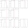	Fig. 6 Same as Fig. 5 but for 4 kpc <R< 5 kpc.
In the text

	Fig. 7 Same as Fig. 6 but only considering pixels where ICO > 2σ. A similar cut for the central radii would show little effect as the CO signal there is strong.
In the text

	Fig. 8 Quality of fit for model with ICO = 1 ± 0.25 K km s-1, N(H i) = 8 ± 1 × 1020 cm-2, and Kdark = 1 ± 0.25 × 1020 cm-2, assuming that the uncertainty in the dust surface density is 25%. Dotted lines represent, from left to right, constant GDR values of 100, 150, 200, 250. The star at XCO = 4 × 1020 cm-2/ (K km s-1) is the input value but the best fit is far from that.
In the text

	Fig. 9 Optimal retrieved values of XCO (left column) and K (right column) as a function of the CO intensity (before adding noise) and the noise level of the CO observations. Top figures: fiducial model. Middle row: fiducial except H i column density reduced to 4 × 1020 cm-2. Bottom: fiducial except dust uncertainties reduced to 10%.
In the text

	Fig. 10 Test of the Bayesian method. The input values for the simulation are shown as blue lines and these correspond rather well to the peaks of probability distributions determined by the method. The dashed lines indicate the median and ± 1σ and ± 2σ intervals.
In the text

	Fig. 11 Comparison of rapid and full errors-in-variables Bayesian simulations. The solid line represents the equality of the two quantities and the dashed (resp. dotted) lines are constant ratios of 0.25 (resp. 0.5).
In the text

Fig. 12 Results of Bayesian analysis with a 3σ cut in CO and no cap on GDR. Top row is Kdark (left) and uncertainty in Kdark (right), both with the color scale to the right and in units of M⊙/ pc2. The second row is XCO (left) and uncertainty in XCO (right), both with the color scale to the right and in units of M⊙/ pc2 per K km s-1. Bottom row is GDR (left) and uncertainty in GDR (right), both with the color scale to the right. As with the other figures, we have adopted the variable-beta dust surface density shown in Fig. 2.

In the text

	Fig. 13 Radial variation of Kdark, αCO, and GDR for the simulation with a cut at 3σ for the CO but no cap on GDR. The value is computed using the maps in Fig. 12 and weighting each macropixel according to is area within a given radial annulus. The error bars indicate the dispersion within this ring. A divergence of Kdark and GDR can be seen in the outer part.
In the text

	Fig. 14 Maps of the number of pixels in each macropixel for the 0σ (left) and 3σ (right) CO cuts.
In the text

	Fig. 15 Average values for Kdark, XCO, and GDR derived for 0.5 kpc radial bins using the Bayesian method. The black histogram shows results derived with the variable beta of Tabatabaei et al. (2014) and the red uses the standard β = 2 to determine dust temperatures.
In the text

	Fig. 16 As for Fig. 12 but with a 500 cap on GDR. The differences can be seen in the outer parts where some of the high GDR pixels from Fig. 12 which were white because they had values over 500.
In the text

	Fig. 17 Radial variation of Kdark, αCO, and GDR for the simulation with a cut at 3σ for the CO and GDR capped at 500. The value is computed using the maps in Fig. 16 and weighting each macropixel according to is area within a given radial annulus. The error bars indicate the dispersion within this ring.
In the text

Fig. 18 Results of Bayesian analysis with a 0σ cut in CO and GDR limited to 500. Top row is Kdark (left) and uncertainty in Kdark (right), both with the color scale to the right and in units of M⊙/ pc2. The second row is XCO (left) and uncertainty in XCO (right), both with the color scale to the right and in units of M⊙/ pc2 per K km s-1. Bottom row is GDR (left) and uncertainty in GDR (right), both with the color scale to the right. As with the other figures, we have adopted the variable-beta dust surface density shown in Fig. 2.

In the text

Fig. 19 Radial variation of Kdark , αCO, and GDR for the simulation with a cut at 0σ for the CO and GDR capped at 500. The value is computed using the maps in Fig. 18 and weighting each macropixel according to is area within a given radial annulus. The error bars indicate the dispersion within this ring. The comparison with the preceding figures shows that the cap on GDR is critical to avoid diverging values of GDR and Kdark.

In the text

Fig. 20 H2 surface density derived from CO and Kdark derived from the Bayesian analysis. The continuous curve shows ΣH2 based on Fig. 10 of Druard et al. (2014) corrected to a XCO factor of 1.1 Galactic and uncorrected for inclination and helium content. The histograms show the CO dark gas surface density. The solid histogram shows Kdark as derived assuming that all positions have the same dark column as the positions where CO is detected above the threshold. The dashed and dotted histograms represent Kdark assuming that the dark column only is present where CO is detected above the 0σ and 3σ thresholds respectively.

In the text

	Fig. 21 Top: link between H i column density and dust surface density for 3 macro-pixels near the center of M 33. Each color represents the pixel values of N(H i) and Σdust for a single macro-pixel. Bottom: same as above but for 3 macro-pixels between 4 and 5 kpc from the center.
In the text

	Fig. 22 Search for degeneracies between the GDR, XCO, and Kdark in the Bayesian approach. Top panel: XCO (αCO) and Kdark as a function of GDR. Bottom panel: link (or absence) between XCO (αco) and Kdark. Each point represents a pixel in the maps shown in Fig. 16.
In the text

References

- Asplund, M., Grevesse, N., Sauval, A. J., & Scott, P. 2009, ARA&A, 47, 481 [NASA ADS] [CrossRef] [Google Scholar]
- Boquien, M., Calzetti, D., Combes, F., et al. 2011, AJ, 142, 111 [NASA ADS] [CrossRef] [Google Scholar]
- Braine, J., Brouillet, N., & Baudry, A. 1997, A&A, 318, 19 [NASA ADS] [Google Scholar]
- Braine, J., Gratier, P., Kramer, C., et al. 2010, A&A, 518, L69 [NASA ADS] [CrossRef] [EDP Sciences] [Google Scholar]
- Combes, F. 2013, in New Trends in Radio Astronomy in the ALMA Era: The 30th Anniversary of Nobeyama Radio Observatory, eds. R. Kawabe, N. Kuno, & S. Yamamoto, ASP Conf. Ser., 476, 23 [Google Scholar]
- Dickman, R. L., Snell, R. L., & Schloerb, F. P. 1986, ApJ, 309, 326 [NASA ADS] [CrossRef] [Google Scholar]
- Draine, B. T., & Li, A. 2007, ApJ, 657, 810 [NASA ADS] [CrossRef] [Google Scholar]
- Druard, C., Braine, J., Schuster, K. F., et al. 2014, A&A, 567, A118 [NASA ADS] [CrossRef] [EDP Sciences] [Google Scholar]
- Foreman-Mackey, D., Hogg, D. W., Lang, D., & Goodman, J. 2013, PASP, 125, 306 [CrossRef] [Google Scholar]
- Galleti, S., Bellazzini, M., & Ferraro, F. R. 2004, A&A, 423, 925 [NASA ADS] [CrossRef] [EDP Sciences] [Google Scholar]
- Galliano, F., Hony, S., Bernard, J.-P., et al. 2011, A&A, 536, A88 [NASA ADS] [CrossRef] [EDP Sciences] [Google Scholar]
- Gardan, E., Braine, J., Schuster, K. F., Brouillet, N., & Sievers, A. 2007, A&A, 473, 91 [NASA ADS] [CrossRef] [EDP Sciences] [Google Scholar]
- Gielen, C., van Winckel, H., Min, M., et al. 2010, A&A, 515, C2 [NASA ADS] [CrossRef] [EDP Sciences] [Google Scholar]
- Goodman, J., & Weare, J. 2010, Commun. Appl. Math. Comput. Sci., 5 [Google Scholar]
- Gordon, K. D., Roman-Duval, J., Bot, C., et al. 2014, ApJ, 797, 85 [NASA ADS] [CrossRef] [Google Scholar]
- Gratier, P., Braine, J., Rodriguez-Fernandez, N. J., et al. 2010a, A&A, 512, A68 [NASA ADS] [CrossRef] [EDP Sciences] [Google Scholar]
- Gratier, P., Braine, J., Rodriguez-Fernandez, N. J., et al. 2010b, A&A, 522, A3 [NASA ADS] [CrossRef] [EDP Sciences] [Google Scholar]
- Gratier, P., Braine, J., Rodriguez-Fernandez, N. J., et al. 2012, A&A, 542, A108 [NASA ADS] [CrossRef] [EDP Sciences] [Google Scholar]
- Hogg, D. W., Bovy, J., & Lang, D. 2010, ArXiv e-prints [arXiv:1008.4686] [Google Scholar]
- Hunt, L. K., García-Burillo, S., Casasola, V., et al. 2015, A&A, 583, A114 [NASA ADS] [CrossRef] [EDP Sciences] [Google Scholar]
- Kennicutt, R. C., & Evans, N. J. 2012, ARA&A, 50, 531 [NASA ADS] [CrossRef] [Google Scholar]
- Kramer, C., Buchbender, C., Xilouris, E. M., et al. 2010, A&A, 518, L67 [NASA ADS] [CrossRef] [EDP Sciences] [Google Scholar]
- Kruegel, E., & Siebenmorgen, R. 1994, A&A, 288, 929 [NASA ADS] [Google Scholar]
- Lada, C. J., Forbrich, J., Lombardi, M., & Alves, J. F. 2012, ApJ, 745, 190 [NASA ADS] [CrossRef] [Google Scholar]
- Leroy, A. K., Bolatto, A., Gordon, K., et al. 2011, ApJ, 737, 12 [NASA ADS] [CrossRef] [Google Scholar]
- Madau, P., & Dickinson, M. 2014, ARA&A, 52, 415 [NASA ADS] [CrossRef] [Google Scholar]
- Magrini, L., Stanghellini, L., & Villaver, E. 2009, ApJ, 696, 729 [NASA ADS] [CrossRef] [Google Scholar]
- Matsuura, M., Dwek, E., Meixner, M., et al. 2011, Science, 333, 1258 [NASA ADS] [CrossRef] [Google Scholar]
- Mookerjea, B., Israel, F., Kramer, C., et al. 2016, A&A, 586, A37 [NASA ADS] [CrossRef] [EDP Sciences] [Google Scholar]
- Pineda, J. L., Langer, W. D., Velusamy, T., & Goldsmith, P. F. 2013, A&A, 554, A103 [NASA ADS] [CrossRef] [EDP Sciences] [Google Scholar]
- Planck Collaboration XIX. 2011, A&A, 536, A19 [NASA ADS] [CrossRef] [EDP Sciences] [Google Scholar]
- Rémy-Ruyer, A., Madden, S. C., Galliano, F., et al. 2014, A&A, 563, A31 [NASA ADS] [CrossRef] [EDP Sciences] [Google Scholar]
- Sandstrom, K. M., Leroy, A. K., Walter, F., et al. 2013, ApJ, 777, 5 [NASA ADS] [CrossRef] [Google Scholar]
- Sodroski, T. J., Odegard, N., Dwek, E., et al. 1995, ApJ, 452, 262 [NASA ADS] [CrossRef] [Google Scholar]
- Tabatabaei, F. S., Braine, J., Xilouris, E. M., et al. 2014, A&A, 561, A95 [NASA ADS] [CrossRef] [EDP Sciences] [Google Scholar]
- Tielens, A. G. G. M., & Hollenbach, D. 1985, ApJ, 291, 722 [NASA ADS] [CrossRef] [Google Scholar]
- Wolfire, M. G., Hollenbach, D., & McKee, C. F. 2010, ApJ, 716, 1191 [NASA ADS] [CrossRef] [Google Scholar]
- Xilouris, E. M., Tabatabaei, F. S., Boquien, M., et al. 2012, A&A, 543, A74 [NASA ADS] [CrossRef] [EDP Sciences] [Google Scholar]