| Issue |
A&A
Volume 597, January 2017
|
|
|---|---|---|
| Article Number | A5 | |
| Number of page(s) | 28 | |
| Section | Extragalactic astronomy | |
| DOI | https://doi.org/10.1051/0004-6361/201628128 | |
| Published online | 19 December 2016 | |
(Sub)millimetre interferometric imaging of a sample of COSMOS/AzTEC submillimetre galaxies
IV. Physical properties derived from spectral energy distributions
1 Department of PhysicsUniversity of Zagreb, Bijenička cesta 32, 10000 Zagreb, Croatia
e-mail: This email address is being protected from spambots. You need JavaScript enabled to view it.
2 Núcleo de Astronomía, Facultad de Ingeniería, Universidad Diego Portales, Av. Ejército 441, Santiago, Chile
3 Argelander-Institut für Astronomie, Universität Bonn, Auf dem Hügel 71, 53121 Bonn, Germany
4 Infrared Processing and Analysis Center, California Institute of Technology, MC 314-6, Pasadena, CA 91125, USA
5 National Radio Astronomy Observatory, 520 Edgemont Road, Charlottesville, VA 22903, USA
6 Max-Planck-Institut für Astronomie, Königstuhl 17, 69117 Heidelberg, Germany
7 Spitzer Science Center, 314-6 California Institute of Technology, Pasadena, CA 91125, USA
8 Aix-Marseille Université, CNRS, LAM (Laboratoire d’Astrophysique de Marseille), UMR 7326, 13388 Marseille, France
9 Leiden Observatory, Leiden University, PO Box 9531, 2300 RA Leiden, The Netherlands
10 National Radio Astronomy Observatory, 1003 Lopezville Road, Socorro, NM 87801-0387, USA
11 Sorbonne Universités, UPMC Université Paris 6 et CNRS, UMR 7095, Institut d’Astrophysique de Paris, 98bis boulevard Arago, 75014 Paris, France
Received: 14 January 2016
Accepted: 2 September 2016
Abstract
Context. Submillimetre galaxies (SMGs) in the early Universe are potential antecedents of the most massive galaxies we see in the present-day Universe. An important step towards quantifying this galactic evolutionary connection is to investigate the fundamental physical properties of SMGs, such as their stellar mass content (M⋆) and star formation rate (SFR).
Aims. We attempt to characterise the physical nature of a 1.1 mm selected, flux-limited, and interferometrically followed up sample of SMGs in the COSMOS field.
Methods. We used the latest release of the MAGPHYS code to fit the multiwavelength (UV to radio) spectral energy distributions (SEDs) of 16 of the target SMGs, which lie at redshifts z ≃ 1.6−5.3. We also constructed the pure radio SEDs of our SMGs using three different radio bands (325 MHz, 1.4 GHz, and 3 GHz). Moreover, since two SMGs in our sample, AzTEC 1 and AzTEC 3, benefit from previous 12C16O line observations, we studied their properties in more detail.
Results. The median and 16th–84th percentile ranges of M⋆, infrared (8−1000 μm) luminosity (LIR), SFR, dust temperature (Tdust), and dust mass (Mdust) were derived to be log (M⋆/M⊙) = 10.96+ 0.34-0.19, log (LIR/L⊙) = 12.93+ 0.09-0.19, SFR = 856+ 191-310M⊙ yr-1, Tdust = 40.6+ 7.5-8.1 K, and log (Mdust/M⊙) = 9.17+ 0.03-0.33, respectively. We found that 63% of our target SMGs lie above the galaxy main sequence by more than a factor of 3 and, hence, are starbursts. The 3 GHz radio sizes we have previously measured for the target SMGs were compared with the present M⋆ estimates, and we found that the z> 3 SMGs are fairly consistent with the mass–size relationship of z ~ 2 compact, quiescent galaxies (cQGs). The median radio spectral index is found to be α = −0.77+ 0.28-0.42. The median IR-radio correlation parameter is found to be q = 2.27+ 0.27-0.13, which is lower than was measured locally (median q = 2.64). The gas-to-dust mass ratio for AzTEC 1 is derived to be δgdr = 90+ 23-19, while that for AzTEC 3 is 33+ 28-18. AzTEC 1 is found to have a sub-Eddington SFR surface density (by a factor of 2.6+ 0.2-0.1), while AzTEC 3 appears to be an Eddington-limited starburster. The gas reservoir in these two high-z SMGs would be exhausted in only ~ 86 and 19 Myr at the current SFR, respectively.
Conclusions. A comparison of the MAGPHYS-based properties of our SMGs with those of equally bright SMGs in the ECDFS field (the ALESS SMGs) that are 870 μm selected and followed up by ALMA, suggests that the two populations share fairly similar physical characteristics, including the q parameter. The somewhat higher Ldust for our sources (factor of 1.9+ 9.3-1.6 on average) can originate in the longer selection wavelength of 1.1 mm. Although the derived median α is consistent with a canonical synchrotron spectral index, some of our SMGs exhibit spectral flattening or steepening, which can be attributed to different cosmic-ray energy gain and loss mechanisms. A hint of negative correlation is found between the 3 GHz size and the level of starburstiness and, hence, cosmic-ray electrons in more compact starbursts might be more susceptible to free-free absorption. Some of the derived low and high q values (compared to the local median) could be the result of a specific merger or post-starburst phase of galaxy evolution. Overall, our results, such as the M⋆–3 GHz radio size analysis and comparison with the stellar masses of z ~ 2 cQGs in concert with the star formation properties of AzTEC 1 and 3, support the scenario where z> 3 SMGs evolve into the present day giant, gas-poor ellipticals.
Key words: galaxies: evolution / galaxies: formation / galaxies: starburst / galaxies: star formation / radio continuum: galaxies / submillimeter: galaxies
© ESO, 2016
1. Introduction
Submillimetre galaxies (SMGs; e.g. Smail et al. 1997; Hughes et al. 1998; Barger et al. 1998; Eales et al. 1999) are a population of some of the most extreme, dusty, star-forming galaxies in the Universe, and have become one of the prime targets for studying massive galaxy evolution across cosmic time (for a recent review, see Casey et al. 2014). Abundant evidence has emerged that high-redshift (z ≳ 3) SMGs are the potential antecedents of the z ~ 2 compact, quiescent galaxies (cQGs), which ultimately evolve into the present-day massive (M⋆ ≥ 1011M⊙), gas-poor elliptical galaxies (e.g. Swinbank et al. 2006; Fu et al. 2013; Toft et al. 2014; Simpson et al. 2014). A better, quantitative understanding of the interconnected physical processes that drive the aforementioned massive galaxy evolution requires us to determine the key physical properties of SMGs, such as the stellar mass (M⋆) and star formation rate (SFR). Fitting the observed multiwavelength spectral energy distributions (SEDs) of SMGs provides an important tool for this purpose. The physical characteristics derived through SED fitting for a well-defined sample of SMGs, as performed in the present study, can provide new, valuable insights into the evolutionary path from the z ≳ 3 SMG phase to local massive ellipticals. However, these studies are exacerbated by the fact that high-redshift SMGs are also the most dust-obscured objects in the early Universe (e.g. Dye et al. 2008; Simpson et al. 2014).
Further insight into the nature of SMGs can be gained by studying the infrared (IR)-radio correlation (e.g. Helou et al. 1985; Yun et al. 2001) of this galaxy population. On the basis of the relative strength of the continuum emission in the IR and radio wavebands, the IR-radio correlation can provide clues to the evolutionary (merger) stage of a starbursting SMG (Bressan et al. 2002), or it can help identify radio-excess active galactic nuclei (AGNs) in SMGs (e.g. Del Moro et al. 2013). Moreover, because submillimetre-selected galaxies have been identified over a wide redshift range, from z ~ 0.1 (e.g. Chapman et al. 2005) to z = 6.34 (Riechers et al. 2013), it is possible to examine whether the IR-radio correlation of SMGs has evolved across cosmic time. A potentially important bias in the IR-radio correlation studies is the assumption of a single radio spectral index (usually the synchrotron spectral index ranging from α = −0.8 to −0.7, where α is defined at the end of this section) for all individual sources in the sample. Hence, the sources that have steep (α ≲ −1), flat (α ≈ 0), or inverted (α> 0) radio spectra will be mistreated under the simplified assumption of a canonical synchrotron spectral index (see e.g. Thomson et al. 2014). As implemented in the present work, this can be circumvented by constructing the radio SEDs of the sources when there are enough radio data points available, and by deriving the radio spectral index values for each individual source.
Ultimately, a better understanding of the physics of star formation in SMGs (and galaxies in general) requires us to investigate the properties of their molecular gas content, which is the raw material for star formation. Two of our target SMGs benefit from previous 12C16O spectral line observations (Riechers et al. 2010; Yun et al. 2015), which, when combined with their SED-based properties derived here, enable us to investigate a multitude of their interstellar medium (ISM) and star formation properties.
In this paper, we study the key physical properties of a sample of SMGs in the Cosmic Evolution Survey (COSMOS; Scoville et al. 2007) deep field through fitting their panchromatic SEDs. The layout of this paper is as follows. In Sect. 2, we describe our SMG sample, previous studies of their properties, and the employed observational data. The SED analysis and its results are presented in Sect. 3. A comparison with previous literature and discussion of the results are presented in Appendix C and Sect. 4, respectively; Appendices A and B contain photometry tables and details of our target sources. The two high-redshift SMGs in our sample that benefit from CO observations are described in more detail in Appendix D. In Sect. 5, we summarise the results and present our conclusions. The cosmology adopted in the present work corresponds to a spatially flat ΛCDM (Lambda cold dark matter) Universe with the present-day dark energy density parameter ΩΛ = 0.70, total (dark plus luminous baryonic) matter density parameter Ωm = 0.30, and a Hubble constant of H0 = 70 km s-1 Mpc-1. A Chabrier (Chabrier 2003) Galactic-disk initial mass function (IMF) is adopted in the analysis. Throughout this paper we define the radio spectral index, α, as Sν ∝ να, where Sν is the flux density at frequency ν.
2. Data
2.1. Source sample: the JCMT/AzTEC 1.1 mm selected SMGs
The target SMGs of the present study were first uncovered by the λobs = 1.1 mm survey of a COSMOS subfield (0.15 deg2 or 7.5% of the full 2 deg2 COSMOS field) carried out with the AzTEC bolometer array on the James Clerk Maxwell Telescope (JCMT) by Scott et al. (2008). The angular resolution of these observations was 18″ (full width at half maximum; FWHM). The 30 brightest SMGs that comprise our parent flux-limited sample were found to have de-boosted flux densities of S1.1 mm ≥ 3.3 mJy, which correspond to signal-to-noise ratios of S/N1.1 mm ≥ 4.0 (see Table 1 in 2008). The 15 brightest SMGs, called AzTEC 1–15 (S/N1.1 mm = 4.−8.3), were followed up with the Submillimetre Array (SMA) at 890 μm (2″ resolution) by Younger et al. (2007, 2009; see also Younger et al. 2008, 2010; Smolčić et al. 2011; Riechers et al. 2014; M. Aravena et al., in prep.); all the SMGs were interferometrically confirmed. Miettinen et al. (2015a; hereafter Paper I) presented the follow-up imaging results of AzTEC 16−30 (S/N1.1 mm = 4.0−4.5) obtained with the Plateau de Bure Interferometer (PdBI) at λobs = 1.3 mm ( resolution). In Paper I, we combined our results with the Younger et al. (2007, 2009) SMA survey results, and concluded that ~ 25% of the 30 single-dish detected sources AzTEC 1–30 are resolved into multiple (two to three) components at an angular resolution of about ~ 2″, making the total number of interferometrically identified SMGs to be 39 among the 30 target sources (but see Appendix B.3 herein for a revised fraction). Moreover, the median redshift of the full sample of these interferometrically identified SMGs was determined to be z = 3.17 ± 0.27, where the quoted error refers to the standard error of the median computed as
  , where σ is the sample standard deviation, and N is the size of the sample (e.g. Lupton 1993). This high median redshift of our target SMGs can be understood to be caused by the long observed wavelength of λobs = 1.1 mm at which the sources were identified (Béthermin et al. 2015; see also Strandet et al. 2016). The corresponding median rest-frame wavelength probed by 1.1 mm observations, λrest ≃ 264μm, is very close to that of the classic 850 μm selected SMGs lying at a median redshift of z ≃ 2.2 (λrest ≃ 266μm; Chapman et al. 2005).
Miettinen et al. (2015b; hereafter Paper II) found that ~ 46% of the present target SMGs are associated with νobs = 3 GHz radio emission on the basis of the observations taken by the Karl G. Jansky Very Large Array (VLA) COSMOS 3 GHz Large Project, which is a sensitive (1σ noise of 2.3 μJy beam-1), high angular resolution ( ) survey (PI: V. Smolčić; Smolčić et al. 2016b). In Paper II, we focused on the spatial extent of the radio-emitting regions of these SMGs, and derived a median deconvolved angular FWHM major axis size of
  . For a subsample of 15 SMGs with available spectroscopic or photometric redshifts we derived a median linear major axis FWHM of 4.2 ± 0.9 kpc. In a companion paper by Smolčić et al. (2016a; hereafter Paper III), we present the results of the analysis of the galaxy overdensities hosting our 1.1 mm selected AzTEC SMGs. In the present follow-up study, we derive the fundamental physical properties of our SMGs, including M⋆, total infrared (IR) luminosity (λrest = 8−1000μm), SFR, and dust mass. In addition, we study the centimetre-wavelength radio SEDs of the sources, and address the relationship between the IR and radio luminosities, i.e. the IR-radio correlation among the target SMGs. These provide an important addition to the previously determined redshift and 3 GHz size distributions (Papers I and II), and allow us to characterise the nature of these SMGs further.
The target SMGs, their coordinates, and redshifts are tabulated in Table 1. The ultraviolet (UV)-radio SEDs in the present work are analysed for a subsample of 16 (out of 39) SMGs whose redshift could have been determined through spectroscopic or photometric methods (i.e. not only a lower z limit), and that have a counterpart in the employed photometric catalogues described in Sect. 2.2 below. We note that an additional nine sources (AzTEC 2, 11-N, 14-W, 17b, 18, 19b, 23, 26a, and 29b) have a zspec or zphot value available, but they either do not have sufficiently wide multiwavelength coverage to derive a reliable UV–radio SED, or no meaningful SED fit could otherwise be obtained (see Appendix B.2 for details). The remaining 14 sources have only lower redshift limits available (owing to the lack of counterparts at other wavelengths). As we have already pointed out in Papers I and II (see references therein), AzTEC 1–30 have not been detected in X-rays, and hence do not appear to harbour any strong AGNs. In Paper II, we found that the νobs = 3 GHz radio emission from our SMGs is powered by processes related to star formation rather than by AGN activity (the brightness temperatures were found to be TB ≪ 104 K). This is further supported by the fact that none of these SMGs were detected with the Very Long Baseline Array (VLBA) observations at a high, milliarcsec resolution at νobs = 1.4 GHz (N. Herrera Ruiz et al., in prep.). Furthermore, in the present paper we find no evidence of radio-excess emission that would imply the presence of AGN activity (Sect. 4.4). We also note that Riechers et al. (2014) did not detect the highly excited J = 16−15 CO line (the upper-state energy Eup/kB = 751.72 K) towards AzTEC 3 in their Atacama Large Millimetre/submillimetre Array (ALMA) observations, which is consistent with the finding of no AGN contributing to the heating of the gas.
Source list.
2.2. Multiwavelength photometric data
Our SMGs lie within the COSMOS field and, hence, benefit from rich panchromatic datasets across the electromagnetic spectrum (from X-rays to radio). To construct the SEDs of our sources, we employed the most current photometric catalogue COSMOS2015, which consists of extensive ground and space-based photometric data in the optical to mid-IR wavelength range (Laigle et al. 2016; see also Capak et al. 2007; Ilbert et al. 2009).
The wide-field imager, MegaCam (Boulade et al. 2003), mounted on the 3.6 m Canada-France-Hawaii Telescope (CFHT), was used to perform deep u∗-band (effective wavelength λeff = 3911 Å) observations. Most of the wavelength bands were observed using the Subaru Prime Focus Camera (Suprime-Cam) mounted on the 8.2 m Subaru telescope (Miyazaki et al. 2002; Taniguchi et al. 2007, 2015). These include the six broadband filters B, g+, V, r, i+, and z++, the 12 intermediate-band filters IA427, IA464, IA484, IA505, IA527, IA574, IA624, IA679, IA709, IA738, IA767, and IA827, and the two narrow bands, NB711 and NB816. The Subaru/Hyper Suprime-Cam (Miyazaki et al. 2012) was used to perform observations in its HSC-Y band (central wavelength λcen = 0.98μm). Near-infrared imaging of the COSMOS field in the Y (1.02 μm), J (1.25 μm), H (1.65 μm), and Ks (2.15 μm) bands is being collected by the UltraVISTA survey (McCracken et al. 2012; Ilbert et al. 2013)1. The UltraVISTA data used in the present work correspond to the data release version 2 (DR2). The Wide-field InfraRed Camera (WIRCam; Puget et al. 2004) on the CFHT was also used for H- and Ks-band imaging. Mid-infrared observations were obtained with the Infrared Array Camera (IRAC; 3.6−8.0 μm; Fazio et al. 2004) and the Multiband Imaging Photometer for Spitzer (MIPS; 24−160 μm; Rieke et al. 2004) on board the Spitzer Space Telescope as part of the COSMOS Spitzer survey (S-COSMOS; Sanders et al. 2007). The IRAC 3.6 μm and 4.5 μm observations used here were taken by the Spitzer Large Area Survey with Hyper Suprime-Cam (SPLASH) during the warm phase of the mission (PI: P. Capak; see Steinhardt et al. 2014). Far-infrared (100, 160, and 250 μm) to sub-mm (350 and 500 μm) Herschel2 continuum observations were performed as part of the Photodetector Array Camera and Spectrometer (PACS) Evolutionary Probe (PEP; Lutz et al. 2011) and the Herschel Multi-tiered Extragalactic Survey (HerMES3; Oliver et al. 2012) programmes.
From the ground-based single-dish telescope data, we used the deboosted JCMT/AzTEC 1.1 mm flux densities reported by Scott et al. (2008, their Table 1). Moreover, for three of our SMGs (AzTEC 5, 9, and 19a) we could use the deboosted JCMT/Submillimetre Common User Bolometer Array (SCUBA-2) 450 μm and 850 μm flux densities from Casey et al. (2013); only a deboosted 850 μm flux density was available for AzTEC 9. More importantly, our SMGs benefit from interferometrically observed (sub)mm flux densities. Among AzTEC 1−15, we used the 890 μm flux densities measured with the SMA by Younger et al. (2007, 2009), while for sources among AzTEC 16−30 we used the PdBI 1.3 mm flux densities from Paper I. AzTEC 1 was observed at 870 μm with ALMA during the second early science campaign (Cycle 1 ALMA project 2012.1.00978.S; PI: A. Karim), and its 870 μm flux density, as measured through a two-dimensional elliptical Gaussian fit, is S870 μm = 14.12 ± 0.25 mJy. We also used the PdBI 3 mm flux density for AzTEC 1 from Smolčić et al. (2011; S3 mm = 0.30 ± 0.04 mJy). Riechers et al. (2014) used ALMA to measure the 1 mm flux density of AzTEC 3 (S1 mm = 6.20 ± 0.25 mJy). Finally, we employed the 1.3 mm flux densities from the ALMA follow-up survey (Cycle 2 ALMA project 2013.1.00118.S; PI: M. Aravena) by M. Aravena et al. (in prep.) of 129 SMGs uncovered in the Atacama Submillimetre Telescope Experiment (ASTE)/AzTEC 1.1 mm survey (Aretxaga et al. 2011). Among the ALMA 1.3 mm detected SMGs there are nine sources in common with the current SED target sources (AzTEC 1, 4, 5, 8, 9, 11-S, 12, 15, and 24b; moreover, AzTEC 2, 6, and 11-N were detected with ALMA at λobs = 1.3 mm).
To construct the radio SEDs for our SMGs, we employed the 325 MHz observations taken by the Giant Meterwave Radio Telescope (GMRT)-COSMOS survey (A. Karim et al., in prep.). We also used the radio-continuum imaging data at 1.4 GHz taken by the VLA (Schinnerer et al. 2007, 2010), and at 3 GHz taken by the VLA-COSMOS 3 GHz Large Project (PI: V. Smolčić; Smolčić et al. 2016b; see also Paper II). Hence, we could build the radio SEDs of our SMGs using data points at three different frequencies.
A selected compilation of mid-IR to mm flux densities of our SMGs are listed in Table A.1, while the GMRT and VLA radio flux densities are tabulated in Table A.2. Because of the large beam size (FWHM) of Herschel/PACS ( and 11″ at 100 and 160 μm, respectively) and SPIRE (18″, 25″, and 36″ at 250, 350, and 500 μm, respectively) observations, the Herschel flux densities were derived using a point spread function fitting method, guided by the known position of Spitzer/MIPS 24 μm sources, i.e. we used the 24 μm prior based photometry (Magnelli et al. 2012) given as part of the COSMOS2015 catalogue (Laigle et al. 2016) whenever possible. Because AzTEC 1, 3, 4, 8, 9, 10, and 17a are reported as non-detections at 24 μm in the COSMOS2015 catalogue, we adopted Herschel flux densities of these sources from the PACS and SPIRE blind catalogues4.
3. Analysis and results
3.1. Spectral energy distributions from UV to radio wavelengths
3.1.1. Method
To characterise the physical properties of our SMGs, we const- ructed their UV to radio SEDs using the multiwavelength data described in Sect. 2.2. The observational data were modelled using the Multiwavelength Analysis of Galaxy Physical Properties code MAGPHYS (da Cunha et al. 2008)5. The commonly used MAGPHYS code has been described in detail in a number of papers (e.g. da Cunha et al. 2008, 2010; Smith et al. 2012; Berta et al. 2013; Rowlands et al. 2014a; Hayward & Smith 2015; Smolčić et al. 2015; da Cunha et al. 2015). Very briefly, MAGPHYS is based on a simple energy balance argument: the UV-optical photons emitted by young stars are absorbed by dust grains in star-forming regions and the diffuse ISM, and the absorbed energy, which heats the grains, is then thermally re-emitted in the IR.
Here we have made use of a new calibration of MAGPHYS, which is optimised to fit the UV-radio SEDs of z> 1 star-forming galaxies simultaneously, and is hence better suited to derive the physical properties of SMGs than the previous versions of the code (see da Cunha et al. 2015). The modifications in the updated version include extended prior distributions of star formation history and dust optical thickness, and the addition of intergalactic medium absorption of UV photons. A simple radio emission component is also taken into account by assuming a correlation between the far-IR (42.5−122.5μm) and radio emission with a qFIR distribution centred at qFIR = 2.34 (the mean value derived by Yun et al. (2001) for z ≤ 0.15 galaxies detected with the Infrared Astronomical Satellite), and a scatter of σ(qFIR) = 0.25 to take possible variations into account (see Sect. 3.5 herein). The thermal free-free emission spectral index in MAGPHYS is fixed at αff = −0.1, while that of the non-thermal synchrotron emission is fixed at αsynch = −0.8. The thermal fraction at rest-frame 1.4 GHz is assumed to be 10%. We note that these assumptions might be invalid for individual SMGs (see our Sects. 3.2, 4.3, and 4.4). The SED models used here assume that the interstellar dust is predominantly heated by the radiation powered by star formation activity, while the possible, though presumably weak, AGN contribution is not taken into account; as mentioned in Sect. 2.1, our SMGs do not exhibit any clear signatures of AGNs in the X-ray or radio emission. Contamination by an AGN is expected to mainly affect the stellar mass determination by yielding an overestimated value (see Hayward & Smith 2015; da Cunha et al. 2015). Hayward & Smith (2015) found that MAGPHYS recovers most physical parameters of their simulated galaxies well, consequently favouring the usage of this SED modelling code. On the other hand, Michałowski et al. (2014) found that MAGPHYS, when employing the Bruzual & Charlot (2003) stellar population models and a Chabrier (2003) IMF, yields stellar masses that are, on average, 0.1 dex (factor of 1.26) higher than the true values of their simulated SMGs. The stellar emission library we used is built on the unpublished 2007 update of the Bruzual & Charlot (2003) models (referred to as CB07), where the treatment of thermally pulsating asymptotic giant branch stars has been improved (see Bruzual 2007).
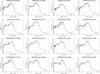 |
Fig. 1 Best-fit panchromatic (UV-radio) rest-frame SEDs of 16 of our target SMGs. The source ID and redshift are shown on the top of each panel. The red points with vertical error bars represent the observed photometric data, and those with downwards pointing arrows indicate the 3σ upper flux density limits (taken into account in the fits). The blue line is the best-fit MAGPHYS model SED from the high-z library (da Cunha et al. 2015). All the SMGs, except AzTEC 21b, are detected in at least one radio frequency (see Fig. 2 for the pure radio SEDs). |
Results of MAGPHYS SED modelling of the target SMGs.
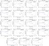 |
Fig. 2 Radio SEDs (on a log-log scale) of 19 of our target SMGs that were detected in at least one of the three observed frequencies of 325 MHz, 1.4 GHz, and 3 GHz (the three data points in each panel with vertical error bars). The downwards pointing arrows show 3σ upper limits. The solid lines show the least squares fits to the data points, and the continuation of the fit is illustrated by the dashed line. The derived spectral index values are shown in each panel. In each panel, the lower x-axis shows the observed frequency, while the upper x-axis gives the corresponding rest-frame frequency (for AzTEC 6 and 27, only a lower z limit is available and, hence, the νrest shown is only a lower limit). |
Radio spectral indices and IR-radio correlation q parameter values.
3.1.2. Spectral energy distribution results
The resulting SEDs are shown in Fig. 1 and the corresponding SED parameters are given in Table 2. Intermediate and narrowband Subaru photometry were not used because their effective wavelengths are comparable to those of the broadband filters, they pass only a small portion of the spectrum, and they can be sensitive to optical spectral line features not modelled by MAGPHYS. Following da Cunha et al. (2015), the flux density upper limits were taken into account by setting the value to zero, and using the upper limit value (here 3σ) as the flux density error. As can be seen in Fig. 1, in a few cases the best-fit model disagrees with some of the observed photometric data points or 3σ upper limits. For example, the Herschel/PACS flux density upper limits (set to 3σ) for AzTEC 4, 5, and 21a lie slightly below the best SED-fit line. As discussed in detail in Paper I, some of our SMGs have uncertain redshifts. Indeed, our initial SED analysis showed that the redshifts we previously adopted for AzTEC 9 and 17a might be underestimated, and the revised redshifts of these SMGs are described in Appendix B.1. Moreover, the SED for AzTEC 3 was fit only using photometry at, and longwards of, the Y band (λrest = 1 620 Å) as the shorter wavelength photometry is likely to be contaminated or dominated by an unrelated foreground (zphot ≃ 1) galaxy, as detailed in Appendix D.2. Finally, as described in Appendix B.2, we could not obtain a meaningful SED fit for the following five SMGs: AzTEC 2, 6, 11-N, 19b, and 26a.
To calculate the total SFR (0.1–100 M⊙) averaged over the past 100 Myr (Col. 4 in Table 2), we used the standard Kennicutt (1998) relationship scaled to a Chabrier (2003) IMF. The resulting LIR−SFR relationship is given by SFR = 10-10 × LIR [L⊙] M⊙ yr-1. The Kennicutt (1998) calibration assumes an optically thick starburst, and it does not account for contributions from old stellar populations (see Bell 2003). The MAGPHYS code also gives the SFR as an output, and the model allows for the heating of the dust by old stellar populations. We found a fairly good agreement with the 100 Myr-averaged SFRs calculated from LIR and those directly resulting from the SED fit: the ratio SFRIR/SFRMAGPHYS was found to range from 0.94 to 3.43 with a median of  , where the ±errors represent the 16th−84th percentile range. We note that when this comparison was carried out using the SFRMAGPHYS values averaged over the past 10 Myr (rather than 100 Myr), the SFRIR/SFRMAGPHYS ratio was found to lie between 0.70 and 1.36 with a median of
  (consistent with da Cunha et al. 2015). In Col. 5 in Table 2, we give the specific SFR, defined by sSFR ≡ SFR/M⋆. The quantity sSFR is unaffected by the adopted stellar IMF in the case where the newly forming stars have the same IMF as the pre-existing stellar population. The SFR, with respect to that of a main-sequence galaxy of the same stellar mass, is given in Col. 6 in Table 2, and is described in Sect. 3.3. Finally, the dust temperature given in Col. 7 is a new MAGPHYS output parameter in the latest version, and it refers to an average, dust luminosity-weighted temperature (see Eq. (8) in da Cunha et al. 2015, for the formal definition).
Most of the SMGs analysed here only have a photometric redshift estimate available (the following 12 sources: AzTEC 4, 5, 7, 9, 10, 12, 15, 17a, 19a, 21a, 21b, and 24b). As shown in Table 1, some of the photometric redshift uncertainties (here reported as the 99% confidence interval; see e.g. Paper I) are large, and we took those uncertainties into account by fitting the source SED over the quoted range of redshifts using a fine redshift grid of Δz = 0.01. We computed the 16th–84th percentile range of the resulting distribution for each MAGPHYS output parameter listed in Table 2, and propagated those values as the uncertainty estimates on the physical parameters. The uncertainties derived using this approach should be interpreted as lower limits to the true uncertainties. We note that da Cunha et al. (2015) left the redshift as a free parameter in their MAGPHYS analysis, in which case the derived photometric redshift uncertainties could be directly and self-consistently included in the uncertainties of all other output parameters. However, this option is not yet possible in the publicly available version of the MAGPHYS high-z extension (E. da Cunha, priv. comm.).
3.2. Pure radio spectral energy distributions, and spectral indices
To study the radio SEDs of our SMGs, we used the 325 MHz GMRT data, and 1.4 GHz and 3 GHz VLA data as described in Sect. 2.2. The radio SEDs for the SMGs detected in at least one of the three radio frequencies are shown in Fig. 2. A linear least squares regression was used to fit the data points on a log–log scale to derive the radio spectral indices. In most cases (the following 15 sources: AzTEC 1, 4, 5, 6, 7, 8, 10, 11-N, 11-S, 12, 15, 17a, 19a, 24b, and 27) the observed data are consistent with a single power-law spectrum. However, for AzTEC 2 and AzTEC 9 the 3σ upper limit to the 325 MHz flux density lies below a value suggested by the 1.4–3 GHz part of the SED, while in the AzTEC 3 and AzTEC 21a SEDs the 1.4 GHz upper flux density limit lies below the fitted power-law function. Because we only have three data points in our galaxy-integrated radio SEDs, we did not try to fit them with anything more complex than a single power law, such as a broken or curved power law. The derived spectral indices are tabulated in Col. 2 in Table 3. In Paper II, we derived the values of  for our SMGs (see Table 4 therein). Those values are almost identical to the corresponding present values, but the quoted uncertainties differ in some cases because of the difference in the method they were derived. In the present study, the uncertainties represent the standard deviation errors weighted by the flux density uncertainty, while in Paper II the spectral index uncertainty was directly propagated from that associated with the flux densities. For AzTEC 2, the reported spectral index refers to a frequency range between 1.4 and 3 GHz. Also, for AzTEC 21b, we could not constrain the radio spectral index needed in the IR-radio correlation analysis (Sect. 3.5). Hence, for this source we assumed a value of
  to be consistent with the canonical non-thermal synchrotron spectral index range of αsynch ∈ [−0.8, −0.7] (e.g. Niklas et al. 1997; Lisenfeld & Völk 2000; Marvil et al. 2015), but AzTEC 21b is not included in the subsequent radio analysis.
The derived  values contain both lower and upper limits. To estimate the median of these doubly censored data, we applied survival analysis. First, we used the dblcens package for R6, which computes the non-parametric maximum likelihood estimation of the cumulative distribution function from doubly censored data via an expectation-maximisation algorithm. This was used to estimate the contribution of the right-censored data. We then used the Kaplan-Meier (K-M) method to construct a model of the input data by assuming that the left-censored data follow the same distribution as the non-censored values; for this purpose, we used the Nondetects And Data Analysis for environmental data (NADA; Helsel 2005) package for R. Using this method the median of was found to be
  , where the ± uncertainty represents the 16th–84th percentile range. Although the derived median spectral index is fully consistent with the value of αsynch = −0.8 which is assumed in the MAGPHYS analysis, some of the individual nominal values are significantly different, which is reflected as poor fits in the radio regime as shown in Fig. 1. The distribution of the derived values as a function of redshift is plotted in Fig. 3. The large number of censored data points allowed us to calculate the median values of the binned data shown in Fig. 3, but not the corresponding mean values. The binned median data points suggest that there is a hint of decreasing (i.e. steepening) spectral index with increasing redshift. To quantify this dependence, we fit the binned data points using a linear regression line, and derived a relationship of the form
  , where the uncertainty in the slope is based on the standard deviation errors of the spectral index data points. The Pearson correlation coefficient of the binned data was found to be r = −0.99. Hence, a negative relationship is present, but it is not statistically significant.
3.3. Stellar mass-SFR correlation: comparison with the main sequence of star-forming galaxies
In Fig. 4, we plot our SFR values as a function of stellar mass. A tight relationship found between these two quantities is known as the main sequence of star-forming galaxies (e.g. Brinchmann et al. 2004; Noeske et al. 2007; Elbaz et al. 2007; Daddi et al. 2007; Karim et al. 2011; Whitaker et al. 2012; Speagle et al. 2014; Salmon et al. 2015). For comparison, in Fig. 4 we also plot the SFR−M⋆ values for ALMA 870 μm detected SMGs from da Cunha et al. (2015; the so-called ALESS SMGs) who used the same high-z extension of MAGPHYS in their analysis as we have used here. Here, we have limited the da Cunha et al. (2015) sample to those SMGs that are equally bright as our target sources (AzTEC 1–30; see Sect. 4.2 for a detailed description).
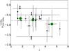 |
Fig. 3 Radio spectral index between 325 MHz and 3 GHz as a function of redshift. The arrows indicate lower and upper limits to |

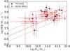 |
Fig. 4 Log-log plot of the SFR vs. stellar mass. The black squares show our AzTEC SMG data points, while the red filled circles show the ALESS SMG data from da Cunha et al. (2015), where the ALESS sample was limited to sources with similar flux densities as our sample (see Sect. 4.2 for details). The dashed lines show the position of the star-forming main sequence at the median redshift of the analysed AzTEC SMGs (z = 2.85; black line) and the flux-limited ALESS sample (z = 3.12; red line) as given by Speagle et al. (2014); the lower and upper black dashed lines indicate a factor of three below and above the main sequence at z = 2.85. |
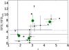 |
Fig. 5 Starburstiness or the distance from the main sequence (parameterised as SFR/SFRMS) as a function of redshift. The blue horizontal dashed line indicates the sample median of 4.6, while the green filled circles represent the mean values of the binned data (each bin contains four SMGs) with the error bars showing the standard errors of the mean values. |
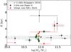 |
Fig. 6 3 GHz radio continuum sizes (radii defined as half the major axis FWHM) derived in Paper II (and scaled to the revised redshifts and cosmology adopted here) plotted against the stellar masses derived in the present work (black squares). The SMGs at z> 3 are highlighted by green star symbols. For comparison, the red squares show the rest-frame UV/optical radii from Toft et al. (2014; also scaled to the present redshifts and cosmology). The upper size limits are indicated by arrows pointing down. The three dashed lines show the mass-size relationship of z ~ 2 compact, quiescent galaxies from Krogager et al. (2014), where the lower and upper lines represent the dispersion in the parameters (see text for details). |
To illustrate how our data compare with the star-forming galaxy main sequence, we overlay the best fit from Speagle et al. (2014), which is based on a compilation of 25 studies, and is given by log (SFR/M⊙ yr-1) = (0.84−0.026 × τuniv)log (M⋆/M⊙)−(6.51−0.11 × τuniv), where τuniv is the age of the Universe in Gyr, i.e. the normalisation rises with increasing redshift. We show the main-sequence position at the median redshift of our analysed SMGs (z = 2.85) and that of the aforementioned ALESS SMG sample (z = 3.12). We also plot the factor of three lines below and above the main sequence at z = 2.85; this illustrates the accepted thickness, or scatter of the main sequence (see e.g. Magdis et al. 2012; Dessauges-Zavadsky et al. 2015). To further quantify the offset from the main sequence, we calculated the ratio of the derived SFR to that expected for a main-sequence galaxy of the same stellar mass, i.e. SFR/SFRMS. The values of this ratio are given in Col. (6) in Table 2, and they range from  to
to  with a median of
  . The values of SFR/SFRMS are plotted as a function of redshift in Fig. 5. The binned data suggest a bimodal behaviour of our SMGs in the sense that the sources at z< 3 are consistent with the main sequence, while those at z> 3 lie above the main sequence. The M⋆-SFR plane of our SMGs is discussed further in Sect. 4.1.
3.4. Stellar mass-size relationship
In Fig. 6, we plot the 3 GHz radio continuum sizes of our SMGs derived in Paper II against their stellar masses derived in the present paper. We also show the rest-frame UV/optical radii for AzTEC 1, 3, 4, 5, 8, 10, and 15 derived by Toft et al. (2014), but which were scaled to our adopted cosmology, and we used the revised redshifts for AzTEC 1, 4, 5, and 15. The radio size data points of the SMGs lying at z> 3 are highlighted by green star symbols in Fig. 6, while the UV/optical sizes are for z ≃ 1.8−5.3 SMGs, out of which 6/7 (86%) lie at z ≳ 2.8. As shown in the figure, with a few exceptions the largest spatial scales of both stellar and radio emission are seen among the highest stellar mass sources (log (M⋆/M⊙) ≥ 11.41). In addition, most of the data points (52% (64%) of all the plotted data (radio sizes)) are clustered within the dispersion of the mass-size relationship of z ~ 2 cQGs derived by Krogager et al. (2014), namely re = γ(M⋆/ 1011M⊙)β, where log (γ/ kpc) = 0.29 ± 0.07 and  for their galaxies with spectroscopic redshifts. The M⋆-size plane analysed here is discussed further in Sect. 4.1.
3.5. Infrared-radio correlation
The quantities derived in the present study allow us to examine the IR-radio correlation among our SMGs (e.g. van der Kruit 1971; de Jong et al. 1985; Helou et al. 1985; Condon et al. 1991; Yun et al. 2001). As usual, we quantify this analysis by calculating the q parameter, which can be defined as (see e.g. Sargent et al. 2010; Magnelli et al. 2015) 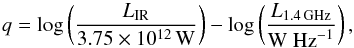 (1)where the value 3.75 × 10¹² is the normalising frequency (in Hz) corresponding to λ = 80μm, and L1.4 GHz is the rest-frame monochromatic 1.4 GHz radio luminosity density. Since our LIR is calculated over the wavelength range of λrest = 8−1000μm, our q value refers to the total-IR value, i.e. q ≡ qTIR. A far-infrared (FIR) luminosity (LFIR) calculated by integrating over λrest = 42.5−122.5μm is sometimes used to define q ≡ qFIR. We note that qTIR = qFIR + log (LIR/LFIR). The 1.4 GHz luminosity density is given by
 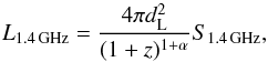 (2)where dL is the luminosity distance. Following Smolčić et al. (2015), the 1.4 GHz flux density was calculated as S1.4 GHz = S325 MHz × (1.4 GHz/325 MHz)α because the observed-frame frequency of νobs = 325 MHz corresponds to the rest-frame frequency of νrest = 1.4 GHz at z = 3.3, which is only a 16% higher redshift than the median redshift of the SMGs analysed here (z = 2.85). Hence, the smallest and least uncertain K correction (1 + z)α to rest-frame 1.4 GHz is needed to derive the value of L1.4 GHz. The derived values of q are listed in Col. 3 in Table 3.
As in the case of (Sect. 3.2), our q values contain both lower and upper limits. Hence, to estimate the sample median, we employed the K-M survival analysis as described in Sect. 3.2. The median q value and the 16th–84th percentile range is found to be  . In Fig. 7, we show the derived q values as a function of redshift and discuss the results further in Sect. 4.4.
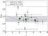 |
Fig. 7 Infrared-radio correlation q ≡ qTIR parameter as a function of redshift. The arrows pointing up and down show the lower and upper limits, respectively. The green filled circles represent the survival analysis-based mean values of the binned data (each bin contains five SMGs) with the error bars showing the standard errors of the mean values. The blue dashed line indicates the median value of |
4. Discussion
The SEDs of some of our COSMOS/AzTEC SMGs have already been analysed in previous studies. We discuss those studies and compare their results with ours in Appendix C. AzTEC 1 and 3 both have a gas mass estimate available in the literature (Yun et al. 2015; and Riechers et al. 2010, respectively), which allows us to examine their ISM physical properties in more detail; these two high-redshift SMGs are discussed in more detail in Appendix D. After discussing the stellar mass-SFR and mass-size relationships of our SMGs in Sect. 4.1, we compare the physical properties of our SMGs with those of the ALESS SMGs derived by da Cunha et al. (2015), and discuss the similarities and differences between the two SMG samples in Sect. 4.2. The radio SEDs and IR-radio correlation are discussed in Sects. 4.3 and 4.4, while the present results are discussed in the context of evolution of massive galaxies in Sect. 4.5.
4.1. How do the COSMOS/AzTEC SMGs populate the M⋆-SFR and M⋆-size planes?
4.1.1. Comparison with the galaxy main sequence
We have found that 10 out of the 16 SMGs (62.5% with a Poisson counting error of 19.8%) analysed here lie above the main sequence with SFR/SFRMS> 3. AzTEC 8 is found to be the most significant outlier with a SFR/SFRMS ratio of about 13. The remaining 6 SMGs have SFR/SFRMS ≃ 0.3−2.4 and, hence, lie on or within the main sequence. Our result is consistent with previous studies where some of the SMGs are found to be located on or close to the main sequence (at the high-mass end), while a fair fraction of SMGs (especially the most luminous objects) are found to lie above the main sequence (e.g. Magnelli et al. 2012; Michałowski et al. 2012; Roseboom et al. 2013; da Cunha et al. 2015; Koprowski et al. 2016). This suggests that SMGs are a mix of populations of two star formation modes, namely normal-type star-forming galaxies and starbursts. Hydrodynamic simulations have also suggested that the SMG population can be divided into two subpopulations consisting of major-merger driven starbursts and disk galaxies where star formation, while possibly driven by mergers or smooth gas accretion, is occuring more quiescently (e.g. Hayward et al. 2011, 2012, and references therein).
4.1.2. Stellar mass-size relationship
As we discussed in Paper II, the rest-frame UV/optical sizes (i.e. the stellar emission size scales), derived by Toft et al. (2014) for a subsample of seven of our SMGs, are smaller than the radio size for AzTEC 4 and 5, in agreement for AzTEC 15, and the upper stellar emission size limits for AzTEC 1, 3, and 8 are larger than their radio sizes, and hence formally consistent with each other; AzTEC 10 was also analysed by Toft et al. (2014), but it is not detected at 3 GHz. A difference between the radio and stellar emission sizes can be partly caused by the fact that rest-frame UV/optical emission can be subject to a strong, and possibly differential dust extinction, and stellar population effects.
In the present work, we revised the stellar masses of the aforementioned seven SMGs, and for those sources where the redshifts used in the analysis were similar, our values are found to be 0.3 to 1.6 (median 0.6) times those from Toft et al. (2014; see Appendix C herein). Despite these discrepancies, the way our SMGs populate the M⋆-size plane shown in Fig. 6 is consistent with the finding of Toft et al. (2014), i.e. the M⋆−R distribution of 3 <z< 6 SMGs is comparable to that of cQGs at z ~ 2. Hence, our result supports the authors’ conclusion that high-z SMGs are potential precursors of the z ~ 2 cQGs, where the quenching of the starburst phase in the former type of galaxies leads to the formation of the latter population (Sect. 4.5).
It is worth noting that five of our z< 3 SMGs plotted in Fig. 6 also exhibit stellar masses and radio sizes that place them in the mass-size relationship of z ~ 2 cQGs from Krogager et al. (2014). While these authors found that the slope and scatter of this mass-size relationship are consistent with the local (z = 0) values, the galaxies grow in size towards lower redshifts (e.g. via mergers). However, as can be seen in Fig. 7 of Krogager et al. (2014, see also references therein), the median size of the quiescent galaxy population at a fixed stellar mass of M⋆ = 1011M⊙ is R ~ 2 kpc in the redshift range z ~ 1.3−2. In the context of massive galaxy evolution, the z< 3 SMGs could potentially evolve into lower redshift (z< 2) cQGs, and then grow in size at later epochs (see Sect. 4.5). As mentioned in Sect. 3.4, there is a hint that the largest 3 GHz radio sizes are found among the most massive of our analysed SMGs (see the ouliers at M⋆ ≳ 2.6 × 10¹¹M⊙ in Fig. 6). While this is not statistically significant, the most extended stellar emission spatial scale is also found for the most massive SMG with available rest-frame, UV-optical size measurement, namely AzTEC 15. Although these largest radio sizes have large error bars, it is possible that the spatially extended radio emission in these massive SMGs is caused by processes that are not related to star formation, such as galaxy mergers leading to magnetic fields that are pulled out from the interacting disks (see Paper II and references therein; O. Miettinen et al., in prep.). Interestingly, all three SMGs that exhibit the largest radio sizes in our sample, namely AzTEC 4, 15, and 21a, are found to lie on the main sequence or only slightly above it (factor of 3.2 for AzTEC 4). But these SMGs have high SFRs of ~ 380−590M⊙ yr-1, which could be induced by gravitational interaction of merging galaxies. This is further supported by the fact that many of our target SMGs exhibit clumpy or disturbed morphologies, or show evidence of close companions at different observed wavelengths, for example in the UltraVISTA NIR images (Younger et al. 2007, 2009; Toft et al. 2014; Paper I).
4.2. Comparison with the physical properties of the ALESS 870 μm selected SMGs
Our main comparison sample of SMGs from the literature is the ALESS SMGs studied by da Cunha et al. (2015). The ALESS SMGs were uncovered in the LABOCA (Large APEX BOlometer CAmera) 870 μm survey of the Extended Chandra Deep Field South (ECDFS) or the LESS survey by Weiß et al. (2009), and followed up with  resolution Cycle 0 ALMA observations (Hodge et al. 2013; Karim et al. 2013). We compare our sample with the da Cunha et al. (2015) study because, firstly, we have also used the new, high-z version of MAGPHYS as first presented and used by da Cunha et al. (2015) to derive the SMG physical properties, which allows for a direct comparison and, secondly, the SMG sample from da Cunha et al. (2015) is relatively large: they analysed the 99 most reliable SMGs detected in the ALESS survey (Hodge et al. 2013).
4.2.1. Description of the basic physical properties of the ALESS SMGs
For their full sample of 99 ALESS SMGs, da Cunha et al. (2015) derived the following median properties (see their Table 1):  ,
,  ,
,  M⊙ yr-1,
  Gyr-1,
  K, and
  . The quoted uncertainties represent the 16th−84th percentile of the likelihood distribution. The value of Ldust reported by da Cunha et al. (2015) refers to the total dust IR (3−1000μm) luminosity, which we have found to be almost equal to LIR with the LIR/Ldust ratio ranging from 0.91 to 0.99 (both the mean and median being 0.95). Also, da Cunha et al. (2015) defined the current SFR over the last 10 Myr, while the corresponding timescale in the present study is 100 Myr. When comparing the MAGPHYS output SFRs, we found that the values averaged over 10 Myr are 1.0 to 4.7 times higher than those averaged over the past 100 Myr, where the mean and median are 2.1 and 1.6, respectively. The authors concluded that the physical properties of the ALESS SMGs are very similar to those of local ultraluminous IR galaxies or ULIRGs (see da Cunha et al. 2010).
For a more quantitative comparison, we limit the da Cunha et al. (2015) sample to those SMGs that have 870 μm flux densities corresponding to our AzTEC 1.1 mm flux density range in the parent sample (AzTEC 1–30), i.e. 3.3 mJy ≤ S1.1 mm ≤ 9.3 mJy. Assuming that the dust emissivity index is β = 1.5, this flux density range corresponds to 7.5 mJy ≤ S870 μm ≤ 21.1 mJy. In the high-z model libraries of MAGPHYS, the value of β is fixed at 1.5 for the warm dust component (30–80 K), while that for the colder (20–40 K) dust is β = 2. A manifestation of this Tdust-dependent β is that scaling the 1.1 mm flux densities to those at 870 μm with a simple assumption of β = 1.5 yields slightly different values than suggested by the MAGPHYS SEDs shown in Fig. 1. The LESS SMGs that fall in the aforementioned flux density range are LESS 1–18, 21–23, 30, 35, and 41, where LESS 1, 2, 3, 7, 15, 17, 22, 23, 35, and 41 were resolved into multiple components with ALMA (Hodge et al. 2013; Karim et al. 2013). The photometric redshifts of these SMGs, as derived by da Cunha et al. (2015), lie in the range of zphot = 1.42−5.22 with a median and its standard error of zphot = 3.12 ± 0.24. This median redshift is only 9.5% higher than that of our analysed SMGs (z = 2.85 ± 0.32). As mentioned in Sect. 3.1.2, the error bars for the parameters of the ALESS SMGs were propagated from the photo-z uncertainties by da Cunha et al. (2015), and they are typically much larger than those of our parameters (see e.g. Fig. 4 herein).
For the aforementioned flux-limited sample, the median values of the physical parameters are  ,
,  ,
,  M⊙ yr-1,
  Gyr-1,
  K, and
  , where we quote the 16th–84th percentile range. All the other quantities, except Tdust, are higher than for the aforementioned full sample, up to a factor of 1.7 for sSFR and Mdust, which is not surprising because the subsample in question is composed of the brightest ALESS SMGs.
Comparison of the physical properties between the target AzTEC SMGs and the equally bright ALESS SMGs.
4.2.2. Comparison of the AzTEC and ALESS SMGs
In what follows, we compare the physical properties of our SMGs with those of the aforementioned flux-limited ALESS sample composed of equally bright sources. The ratios between our median M⋆, Ldust, SFR, sSFR, Tdust, and Mdust values and those of the ALESS SMGs are given in Table 4. For a proper comparison, the comparison of the SFR and sSFR values were carried using the MAGPHYS output values averaged over the past 10 Myr. As can be seen in Table 4, the median values of M⋆ and Tdust are similar, and our median Mdust value is a factor of 1.5 times higher than for the equally bright ALESS SMGs. On the other hand, our dust luminosities and (s)SFR values appear to be about two times higher on average.
We also performed a two-sided Kolmogorov-Smirnov (K-S) test between the aforementioned physical parameter values to check whether our SMGs and the flux-limited ALESS SMG sample could be drawn from a common underlying parent distribution. The null hypothesis was that these two samples are drawn from the same parent distribution. The K-S test statistics and p values for the comparisons of the M⋆, Ldust, SFRMAGPHYS, Tdust, and Mdust values are also given in Table 4. The K-S test results suggest that the underlying stellar mass distribution is the same (p = 0.92), while those of the remaining properties might differ. We note that for Tdust, for which the median value between our AzTEC SMGs and the ALESS SMGs was found to be very similar, the K-S test p value is 0.29, which is the second highest after the stellar mass comparison. Also, the comparison samples are small (16 AzTEC and 25 ALESS sources, respectively), and hence the K-S tests presented here are subject to small number statistics. Nevertheless, we cannot exclude the possibility that at least part of the differences found here is caused by the different selection wavelength (λobs = 1.1 mm versus λobs = 870μm), and different depths of the optical to IR observations available in COSMOS and the ECDFS, although the stellar mass estimates based on the optical regime of the galaxy SED are found to be similar.
da Cunha et al. (2015) found that, at z ≃ 2, about half of the ALESS SMGs (49%) lie above the star-forming main sequence (i.e. SFR/SFRMS> 3), while the other half (51%) are consistent with being at the high-mass end of the main sequence, where the main-sequence definition was also adopted from Speagle et al. (2014). The ALESS SMG sample is flux limited to match our sample limit, which has a median redshift of z = 3.12; for this sample, only 24 ± 10% of the sources are found to have SFR/SFRMS> 3, while the remaining 76 ± 17% lie within a factor of 3 of the main sequence (see our Fig. 4). However, the ALESS sources have significant error bars in their SFR and M⋆ values (propagated from the photo-z uncertainties; da Cunha et al. 2015). The fractions we found for the analysed AzTEC SMGs are nominally more extreme, i.e. 62.5% ± 19.8% are above the main sequence, and 37.5% ± 15.3% are consistent with the main sequence. If we base our analysis on the MAGPHYS output SFRs averaged over 10 Myr, following da Cunha et al. (2015), we find that the fraction of the AzTEC SMGs with SFR/SFRMS> 3 is the same 62.5% ± 19.8% as derived above from the Kennicutt (1998) LIR−SFR calibration.
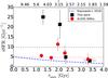 |
Fig. 8 Specific SFR (sSFR) as a function of cosmic time (lower x-axis) and redshift (upper x-axis) for our SMGs and the flux-limited sample of ALESS SMGs. The plotted data points represent the mean values of our data and the ALESS SMG data binned in redshift and sSFR (each of our bin contains four sources, while the ALESS data have five values in each bin). The error bars represent the standard error of the mean. The horizontal dashed lines indicate the full sample median sSFRs of |


In Fig. 8, we plot the sSFR as a function of cosmic time (lower x-axis) and redshift (upper x-axis). For legibility purposes, we only show the binned version of the data; the plotted data points represent the mean values of the full data with four SMGs per bin in our AzTEC sample, and five SMGs per bin in the ALESS sample. The sSFR of the ALESS comparison sample appears to be relatively constant as a function of cosmic time, while our individual SMGs, lying in a similar redshift range, show more scatter with a factor of  higher median sSFR. Our median sSFR is higher by the same nominal factor of
  when comparing the MAGPHYS outputs averaged over 10 Myr; Table 4. The blue dash-dotted line overplotted in the figure represents the sSFR-cosmic time relationship derived by Koprowski et al. (2016). As can be seen, our lowest redshift data point (corresponding to the latest time) lies slightly (by a factor of 1.57) above the normalisation of this relationship, and the second lowest redshift data point, even though it is a factor of 1.82 higher sSFR than suggested by the Koprowski et al. (2016) relationship, is still consistent with this value within the standard error. However, our two highest redshift bins lie at much higher sSFRs than computed from the Koprowski et al. (2016) relationship (by factors of ~ 7), but as mentioned by the authors, their study could not set tight constraints on the sSFR beyond redshift of z ≃ 3 (τuniv = 2.1 Gyr), where many of our SMGs are found. Indeed, as can be seen in Fig. 10 of Koprowski et al. (2016), the scatter of data increases at z> 3, and many data points lie above their derived relationship. It should also be pointed out that our SFRs and stellar masses were derived using a different method than those in Koprowski et al. (2016) and their reference studies, and this could in part explain why our values lie above the Koprowski et al. (2016) sSFR(τuniv) function. On the other hand, while the three lowest redshift ALESS data points shown in Fig. 8 show a trend similar to ours, with a jump in sSFR near z ≃ 3, the two highest redshift ALESS bins are only by factors of 1.43–1.56 above the Koprowski et al. (2016) relationship. Larger, multi-field samples of SMGs are required to limit cosmic variance, and examine the evolution of the sSFR of SMGs as a function of cosmic time further, particularly at z ≳ 3.
Figure 9 plots the dust-to-stellar mass ratio as a function of redshift for our SMGs and the comparison ALESS SMG sample. The median values for these samples are  and
and  , respectively, where the quoted uncertainties represent the 16th–84th percentile range. The binned data points shown in Fig. 9 show a hint of decreasing dust-to-stellar mass ratio towards higher redshifts. The AzTEC (ALESS) data points suggest a linear regression of the form Mdust/M⋆ ∝ −(0.006 ± 0.003) × z (Mdust/M⋆ ∝ −(0.002 ± 0.002) × z), with a Pearson r of −0.68 (−0.86). These trends are not statistically significant, but the fact that both the samples show a comparable behaviour is indicative of a star formation and dust production history that is fairly similar between the AzTEC and ALESS SMGs; hence, this suggests a similar level of metallicity, which is not surprising given that these SMGs lie at the same cosmic epoch.
Thomson et al. (2014) studied the radio properties of the ALESS SMGs. They used 610 MHz GMRT and 1.4 GHz VLA data, and derived a median ± standard error radio spectral index of  for a sample of 52 SMGs. Again, if we limit this comparison sample to those sources that are equally bright as ours, we derive a median spectral index of
  from the values reported in their Table 3 (survival analysis was used to take the lower limits into account). This is the same as for their full sample and is also consistent with our median value of , although our observed frequency range is broader.
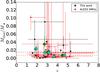 |
Fig. 9 Dust-to-stellar mass ratio as a function of redshift for our SMGs and the flux-limited ALESS SMGs. The green filled circles represent the mean values of the binned AzTEC data (each bin contains four SMGs), while the cyan filled circles represent the mean values of the binned ALESS data (each bin contains five SMGs). The error bars of the binned data points represent the standard errors of the mean values. The horizontal dashed lines indicate the corresponding median values of |


4.3. Properties of radio SEDs
4.3.1. Radio continuum spectra of star-forming galaxies
The radio continuum emission arising from a star-forming galaxy can be divided into two main components: the thermal free-free emission (bremsstrahlung) from H ii regions and non-thermal synchrotron emission from relativistic cosmic-ray electrons. Both of these emission mechanisms are directly linked to the evolution of high-mass stars: a newly forming, high-mass star photoionises its surrounding medium to create an H ii region, while the explosive deaths of high-mass (> 8M⊙) stars, i.e. supernovae and their remnants, are associated with shock fronts that can accelerate cosmic-ray particles to relativistic energies.
While a typical synchrotron spectral index is αsynch ∈ [−0.8, −0.7] (Sect. 3.2, and references therein), that of thermal free-free emission is about seven to eight times flatter, i.e. αff = −0.1. At low frequencies of νrest< 30 GHz the total radio emission is expected to be dominated by the non-thermal synchrotron component, while at higher frequencies (up to about 100 GHz) the thermal emission component makes a larger contribution of the total observed radio wave emission (e.g. Condon 1992; Niklas et al. 1997). The radio flux density at 33 GHz might be affected by the anomalous dust emission, but its significance in the galaxy-integrated measurements is unclear (Murphy et al. 2010). Because of the thermal emission, the radio spectrum exhibits flattening towards higher frequencies. Besides this effect, the low-frequency regime of a radio SED (νrest ≲ 1 GHz) can also exhibit flattening because the free-free optical thickness increases (τ ∝ ν-2.1), and hence the free-free absorption due to ionised gas becomes important.
On the other hand, cosmic-ray electrons suffer from a number of cooling or energy-loss mechanisms. These include synchrotron radiation, inverse-Compton (IC) scattering, ionisation, and bremsstrahlung losses (e.g. Murphy 2009; Paper II and references therein), all of which can shape the radio SED, i.e. modify the spectral index. For example, besides the free-free absorption, ionisation energy losses can flatten the radio spectrum towards lower frequencies (<1 GHz; e.g. Thompson et al. 2006). These energy-loss mechanisms are dependent on the physical properties of the galaxy, such as the magnetic field strength, neutral gas density, and the energy density of the radiation field (e.g. Basu et al. 2015; Paper II and references therein). Moreover, the IC losses at high redshifts can be aided by IC losses off the cosmic microwave background (CMB) photons, because the CMB energy density goes as uCMB ∝ (1 + z)4.
Because the aforementioned physical properties (magnetic field strength, density, etc.) have spatial gradients within the galaxy, the interpretation of the observed galaxy-integrated radio SEDs can become difficult (Basu et al. 2015). However, measurements of the radio spectral index over different frequency ranges can provide useful information about the energy loss and gain mechanisms of the leptonic (e±) cosmic-ray population. In the next subsection, we attempt to classify our SMGs into different categories on the basis of the observed radio spectral indices.
4.3.2. Radio spectral energy distribution classification
To classify our SMGs into different radio SED categories, we define the following three classes: I is the classic synchrotron spectrum (αsynch ≃ −0.8...−0.7), II is the flattened radio spectrum, and III is the steepened radio spectrum. The classification in the observed-frame frequency interval of 325 MHz–3 GHz is provided in Table 5. Seven of our sources agree with a canonical synchrotron spectrum (our category I), while the remaining 11 fall into a category II or III with a 5:6 proportion. We note that AzTEC 3, 10, 21a, and 27 exhibit a nominal spectral index of α< −1.0 (and AzTEC 2 has  ), and these sources could also be classified as ultra-steep spectrum sources (Thomson et al. 2014, 2015).
In the next subsection, we examine the contribution of the thermal free-free emission to the flattest radio spectrum found in the present study.
Classification of the target SMGs into different radio SED categories in the observed frequency interval 0.325–3 GHz.
4.3.3. Thermal fraction
Considering the contribution of the thermal free-free emission to the derived spectral indices, the highest rest-frame frequency probed in the present study is 18.9 GHz, which corresponds to νobs = 3 GHz at the redshift of AzTEC 3 (zspec ≃ 5.3). However, AzTEC 3 has one of the steepest spectral indices derived here (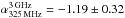 ), although the non-detection at 1.4 GHz could be an indication of a flattening towards higher frequencies (
 ). On the other hand, the flattest index found here is
  for AzTEC 4, which might be an indication that the observed-frame 3 GHz flux density has a contribution from thermal free-free emission. To quantify the level of this free-free contribution, we can translate the LIR-based SFR into the thermal luminosity using Eq. (11) of Murphy et al. (2011), which for a Chabrier (2003) IMF scaling can be written as
 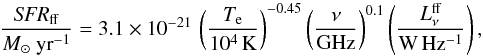 (3)where Te is the electron temperature, which is here set to 104 K. For AzTEC 4, for which the nominal SFR is 380M⊙ yr-1, we obtain a luminosity density of ~ 1 × 10²³ W Hz-1 at the rest-frame frequency νrest = 8.4 GHz (corresponding to νobs = 3 GHz). By comparing this with the radio luminosity density calculated using the observed 3 GHz flux density (see our Eq. (2)), we estimate the thermal fraction to be > 33% for AzTEC 4 at νobs = 3 GHz; the lower limit results from the lower limit used in the calculation. Although the thermal contribution makes the derivation of the non-thermal spectral index more uncertain, our result demonstrates that it also offers a possibility to estimate the SFR of high-z galaxies more directly than relying on the IR-radio correlation. The high sensitivity of the future facilities, such as the Square Kilometre Array7, has the potential to use thermal free-free emission as a reliable, dust-unbiased SFR tracer.
4.3.4. Radio characteristics and the offset from the main sequence
Finally, because most (63%) of our SMGs are found to be starbursts (Sect. 4.1.1), we compare our results with Murphy et al. (2013) who found that the radio spectral indices of galaxies flatten with increasing distance above the galaxy main sequence. The authors interpreted this to mean that compact starbursts are more optically thick in the radio, i.e. because free-free absorption is more important in these systems ( , where ne is the electron density). To test whether our SMGs exhibit such a trend, in the top panel in Fig. 10 we plot our values as a function of the starburstiness parameter SFR/SFRMS. As can be seen, no trend is discernible in Fig. 10. Also, in Paper II we did not find a correlation between the 3 GHz radio sizes of our SMGs and (see Fig. 4 therein)
If the scenario proposed by Murphy et al. (2013) plays out, then one might expect to see a correlation between the size of a galaxy and its distance from the main sequence. To see if this is the case for our SMGs, in the bottom panel in Fig. 10 we plot the 3 GHz radio sizes from Paper II as a function of SFR/SFRMS. Indeed, we see a possible hint that more compact sources are those that lie the furthest away from the main sequence. Interestingly, the largest radio-emitting sizes are seen among SMGs within or near the main sequence (SFR/SFRMS ≲ 3), although the SMGs with a radio size that is close to the sample median size are also found within the main-sequence envelope. Hence, no firm conclusions can be drawn on the basis of current data.
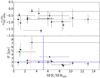 |
Fig. 10 Top: radio spectral index between 325 MHz and 3 GHz as a function of starburstiness or the distance from the main sequence (parameterised as SFR/SFRMS). For reference, the horizontal dashed line indicates the median spectral index value of |

4.4. The IR-radio correlation
4.4.1. Comparison with literature data
The IR-radio q parameters we derived, ranging from q> 1.64 to q = 2.82 ± 0.18 with a median of  , exhibit a hint of negative correlation with redshift (see Sect. 3.5, and the binned data in Fig. 7).
Thomson et al. (2014) reported a median qTIR of 2.56 ± 0.05 for their ALESS SMGs. However, to compute q Thomson et al. (2014) used the IR luminosities derived by Swinbank et al. (2014). Hence, we recalculated the q values for the flux-limited comparison sample using the Ldust values (and photo-z values) derived by da Cunha et al. (2015), and the 610 MHz GMRT flux densities from Thomson et al. (2014) (following our Eqs. (1) and (2) modified for νobs = 610 MHz). We adopted a spectral index of α = −1.57 ± 0.08 derived through stacking by Thomson et al. (2014) for the radio non-detected (at both 610 MHz and 1.4 GHz) ALESS SMGs. The authors reported upper q limits for the radio non-detected SMGs in their Table 1, but in the case of an upper limit to S610 MHz, the corresponding q value becomes a lower limit. The median q we derived this way is 2.29 ± 0.09, where we quote the standard error of the median. Because this value refers to the total dust luminosity (3−1000μm), the total-IR q is slightly lower. Given that the ratio of our median q value to the recalculated ALESS q is 0.99, we conclude that the IR-radio correlation parameter is not significantly different between our SMGs and the equally bright ALESS SMGs.
Similar to Thomson et al. (2014), Barger et al. (2012) reported an average qTIR value of 2.51 ± 0.01 for their sample of five SCUBA 850 μm identified SMGs at z = 2−4 in the Great Observatories Origins Deep Survey-North (GOODS-N). The AzTEC 1.1 mm flux densities of these SMGs lie in the range of S1.1 mm = (1.9 ± 1.4)−(5.4 ± 1.1) mJy (see Table 6 in Barger et al. 2012), and they are generally fainter at λobs = 1.1 mm than our target SMGs with  mJy (2008). Additionally, because Barger et al. (2012) assumed a radio spectral index of α = −0.8, and used a Arp 220 SED-based relationship of LIR = 1.42 × LFIR in their calculation, a direct comparison with our qTIR calculation is not feasible.
The average FIR-based qFIR values derived for SMGs lying at median redshifts of z ~ 2−2.5 and without AGN signatures are usually found to be about 2.0–2.2, which are comparable with those of other types of star-forming galaxies at similar redshifts (e.g. Kovács et al. 2006; Magnelli et al. 2010; Alaghband-Zadeh et al. 2012). For our SMGs, 36% to 90% of the total-IR luminosity is found to emerge in the FIR, with a mean (median) percentage of 75% (80%). Hence, our median qFIR can be derived to be about 2.17, in excellent agreement with previous results.
4.4.2. Evolution of the IR-radio correlation
The question then arises as to what is causing the relatively low qTIR in our (and ALESS) SMGs with respect to the local Universe median value of qTIR = 2.64 (see Bell 2003; Sargent et al. 2010). One possible explanation is related to the dynamical/evolutionary stage of the SMG system. The models by Bressan et al. (2002) predict that the q parameter reaches its minimum value during the post-starburst phase. The authors suggested that this evolutionary effect is due to radio emission fading more slowly after an intense burst of star formation than the (F)IR emission, which is manifested as an apparent radio excess or lower q value. Because SMGs are potentially driven by mergers (e.g. Tacconi et al. 2008; Engel et al. 2010), some of the low q values we have observed suggest that we are observing the target SMG during the post-starburst phase.
Schleicher & Beck (2013) also discussed the possibility of accretion/merger-driven turbulence enhancing the magnetic field strength. If an SMG is driven by a major merger, this could be one mechanism to yield a low q value. It is also possible that environmental effects increase the galactic magnetic field strength and/or reaccelerate cosmic rays, hence causing an excess in radio emission, which lowers the q value (Miller & Owen 2001; Reddy & Yun 2004; Murphy et al. 2009). On the other hand, the value of qTIR we derived for AzTEC 8, i.e. 2.82 ± 0.18, is relatively high compared to the local median value. An elevated qTIR can result from a recent starburst phenomenon, where the synchrotron emission is generated with a time delay (due to the generation of relativistic electrons and/or magnetic field) with respect to the stellar radiation field that heats the dust (Roussel et al. 2003).
Some previous studies have found a moderate evolution of q as a function of redshift (Ivison et al. 2010a,b; Magnelli et al. 2010; Casey et al. 2012; Magnelli et al. 2015; see also Delhaize et al. 2016). For instance, Magnelli et al. (2015) found a statistically significant redshift evolution of the form qFIR = (2.35 ± 0.08) × (1 + z)− 0.12 ± 0.04 for their M⋆ selected, multi-field sample of 0 <z< 2.3 galaxies (including COSMOS), in agreement with that found earlier by Ivison et al. (2010a) for 250 μm selected galaxies at z = 0.038−2.732, i.e. qTIR ∝ (1 + z)− 0.15 ± 0.03. The latter relationships are overplotted in Fig. 7, and normalised to yield the local Universe median value of qTIR(z = 0) = 2.64. We note that the slope of the qTIR(z) curves becoming shallower with increasing z is consistent with a turbulent dynamo theory prediction by Schober et al. (2016).
As can be seen in Fig. 7, our binned SMG data show a weak hint of decreasing evolution in qTIR as a function of cosmic time. A linear regression yields a relationship of the form qTIR ∝ −(0.050 ± 0.060) × z, with a Pearson correlation coefficient of r = −1. Hence, the decreasing trend seen here is not statistically significant. The two lowest redshift bins at z = 2.04 and z = 2.93 are consistent within the standard errors with the nominal q = q(z) relationships of Ivison et al. (2010a) and Magnelli et al. (2015). Our highest redshift binned data point at z = 4.23 lies above those relationships. The ALESS SMGs do not exhibit a (negative) correlation in the qTIR-z plane (Thomson et al. 2014; see Fig. 3 therein).
It is not clear what would cause a trend of decreasing q with redshift. One possibility is an erroneous radio K correction for higher redshift sources due to an increasing thermal free-free contribution to the observed emission (Delhaize et al. 2016). In the present work, we have minimised the K correction by using the observed-frame 325 MHz radio flux densities (Sect. 3.5). If, however, the trend as a function of cosmic time is physical, the question arises whether it is driven by an enhanced radio emission or a depressed IR emission from dust at higher redshifts. If the ISM density of galaxies increases towards higher redshifts, the corresponding galactic magnetic field could be stronger, which in turn would lead to a stronger radio synchrotron emission implying a lower q value (Schleicher & Beck 2013). Given the enhanced IC-CMB cooling of cosmic-ray electrons at high redshifts (Sect. 4.3), the associated suppression of synchrotron radiation could even lead to an increase of q towards higher redshifts, but the magnetic field strength in SMGs might be strong enough to compensate this effect (Thomson et al. 2014). One possible interpretation of the weak or even a complete lack of any obvious q(z) trend among SMGs compared to the negative q(z) relationship among less-extreme star-forming galaxies is that the latter type of galaxies exhibit a lower dust content (and hence a lower LIR and q) at higher redshifts (e.g. Capak et al. 2015), while SMGs are rich in dust at all cosmological epochs they are being observed (and hence q does not decrease, or does so only weakly).
4.5. The 1.1 mm selected COSMOS/AzTEC SMGs in the context of massive galaxy evolution
Putting the results from our previous studies and the present one together, we are in a position to discuss our SMGs in the context of the evolution of massive galaxies. Although the SMGs studied in the present work appear to preferentially lie above the galaxy main sequence (63% have a SFR/SFRMS ratio > 3), and can be considered starbursts, a fair fraction of about 38% are consistent with being main-sequence star-forming galaxies. Nevertheless, the high SFRs of ~ 20−1500 M⊙ yr-1 with a median of 508 M⊙ yr-1 derived for these main-sequence SMGs show that a phase of intense star formation is taking place in these galaxies. We also find an indication for an anti-correlation between distance from the main sequence and radio size (Fig. 10, bottom panel). Moreover, as shown in Fig. 5, there is an average trend that z > 3 SMGs have a higher level of starburstiness (SFR/SFRMS ratio) than those SMGs that lie at z < 3. In Paper II, however, we did not find any trend between radio size and redshift of our target SMGs (Fig. 7 therein; see also O. Miettinen et al., in prep.).
As further shown for two of our high-z SMGs AzTEC 1 and AzTEC 3 in Appendix D, an early starburst phase can be characterised by a SFR occuring near or at the Eddington limit within a spatially compact region. Such high SFRs of luminous SMGs are plausibly triggered by a wet merger between gas-rich galaxies, or, perhaps in the case of less luminous SMGs, by gravitational instabilities fuelled by more continuous, cold gas accretion (Narayanan et al. 2009; Dekel et al. 2009; Engel et al. 2010; Wiklind et al. 2014; Narayanan et al. 2015). For example, the AzTEC 11 system, which is composed of two very nearby ( or 12.4 kpc in projection) dust and radio-emitting components, is possibly in the process of merging in a phase before the parent nuclei have fully coalesced (see Paper II, Fig. 2 therein; and O. Miettinen et al., in prep.).
4.5.1. z > 3 SMGs
Our parent sample contains 12 SMGs that lie at z> 3 (6 of which were analysed in the present work), i.e. at the formation epoch of z ~ 2 cQGs (Toft et al. 2014). As shown in Sect. 3.4, a comparison with the stellar mass-size relationship of z ~ 2 cQGs supports an evolutionary link between these high stellar-density systems and our z> 3 SMGs, in accordance with the results of Toft et al. (2014). To further quantify this evolutionary path, we follow the approach of Toft et al. (2014), and compare the stellar mass distributions of our z> 3 SMGs and z ~ 2 cQGs. In Fig. 11, we plot the mass distribution of our z> 3 SMGs, and the stellar masses of the spectroscopically confirmed z ~ 2 cQGs from Krogager et al. (2014, their Table 2). To estimate the final stellar masses of the z> 3 SMGs, we adopt the CO-based molecular gas masses available for AzTEC 1 and AzTEC 3 (see Appendix D) and, for the remaining four sources, we assume a value of Mgas ~ 1011M⊙, which is the average of the gas masses of AzTEC 1 and 3. Following Toft et al. (2014), we assumed that 10% of the gas mass is converted into stars by the end of the starburst; this star formation efficiency is based on the hydrodynamic simulations by Hayward et al. (2011) as described in Toft et al. 2014. The time interval between z> 3 and z ~ 2 is ≳ 1.1 Gyr, which is much longer than the gas depletion timescale in SMGs; for comparison, the depletion timescale we derived for AzTEC 1 and AzTEC 3 is only  Myr and
  Myr, respectively (Appendix D).
The derived final stellar mass distribution is shown by the blue histogram in Fig. 11. A two-sided K-S test between this mass distribution and the Krogager et al. (2014) cQG M⋆ distribution yielded a K-S test statistic of D = 0.36 and a p value of p = 0.55, suggesting that the two distributions might share a common parent distribution, which would further support the evolutionary link between z> 3 SMGs and z ~ 2 cQGs. However, given the small sample sizes, this comparison should be considered with caution in mind.
As another gas mass estimate (for the sources other than AzTEC 1 and 3), we used the method adopted by Toft et al. (2014), namely the gas-to-dust mass ratio-metallicity (δgdr−Z) relationship derived by Leroy et al. (2011) in combination with the stellar mass-metallicity (M⋆−Z) relationship from Genzel et al. (2012, and references therein). Using the MAGPHYS-based M⋆ and Mdust values, we could then estimate the gas masses and, hence, the final stellar masses under the assumption of a 10% star formation efficiency. The resulting distribution is shown by the magenta dashed histogram in Fig. 11. The median values of the two estimated final stellar mass distributions (the blue and magenta dashed histograms) are the same (log (M⋆/M⊙) = 10.97), and a K-S test performed between the final stellar mass distribution shown by the magenta dashed line and the z ~ 2 cQG M⋆ distribution yielded the same results as above (D = 0.36 and p = 0.55). We emphasise, however, that larger sample sizes are required to better test the validity of the aforementioned stellar mass-metallicity relationship because it is based on the analysis of z ~ 2 galaxies and, hence, its applicability for z> 3 SMGs is questionable (see also Toft et al. 2014). Indeed, the gas-to-dust mass ratios derived through the empirical relationships for AzTEC 1 and 3 are 123 and 119, respectively, which are about 1.4 and 3.6 times higher than the observed values (Appendix D).
At this point, we conclude that on the basis of the mass-size relationship and the stellar mass distribution analyses presented here, the evolutionary connection between z> 3 SMGs and z ~ 2 cQGs seems possible, as proposed by Toft et al. (2014). The subsequent growth of z ~ 2 cQGs through minor dry (gas-poor) mergers can then turn the z ~ 2 cQGs into the giant ellipticals seen in the present-day Universe (Toft et al. 2014).
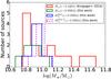 |
Fig. 11 Stellar mass distribution of our z> 3 SMGs (green histogram), and z ~ 2 cQGs (2014; red histogram). The blue histogram shows the distribution of the final stellar masses of the z> 3 SMGs by assuming that 10% of their putative gas mass content is converted into stars by the end of the ongoing starburst event, while the magenta dashed histogram represents the final stellar mass distribution where Mgas is based on the mass-metallicity relationship (see text for details). The CO-based gas mass estimate was adopted for AzTEC 1 and AzTEC 3 (Appendix D). |
4.5.2. Submillimetre galaxies at z ≤ 3
While the above discussion concerns the z> 3 SMG population, most of the SMGs in our parent sample lie at z ≤ 3 (18 sources with either a spectroscopic or photometric redshift, plus seven lower redshift limits at z< 3; 10 sources at z ≃ 1.6−3 were analysed here). Because there are also cQGs at z< 2 (see e.g. the sample of 0.9 <z< 1.6 cQGs in Belli et al. 2014), one could think of a scenario where z ≲ 3 SMGs represent their progenitors. However, our z ≤ 3 SMGs already have a considerable stellar mass content of M⋆ ~ 1.8 × 10¹⁰−4.9 × 10¹¹M⊙ with a median of 2.3 × 10¹¹M⊙, while for example the Chabrier (2003) IMF-based stellar masses of the 0.9 <z< 1.6 cQGs from Belli et al. (2014) are M⋆ ~ 1.9 × 10¹⁰−2.2 × 10¹¹M⊙ with a median of 7 × 10¹⁰M⊙.
Since the stellar masses of our z ≤ 3 SMGs are already higher on average than those of the Belli et al. (2014) cQGs, an evolutionary link between these two populations seems very unlikely, although our SMG subsample here consists of only ten sources, which prevents us from making any firm conclusions. Yet, it has also been shown that lower redshift (z ≤ 3) SMGs have the potential to evolve into the present-day passive ellipticals (Swinbank et al. 2006; Simpson et al. 2014). For instance, based on the H-band magnitude and space density comparisons and the stellar age analysis of local ellipticals, Simpson et al. (2014) showed that the properties of their sample of 77 ALESS SMGs with a median redshift of zphot = 2.3 and local ellipticals agree well with each other, which strongly supports an evolutionary connection between them. Based on the stellar population ages of quiescent, red z ~ 1.5−2 galaxies (e.g. Whitaker et al. 2013), Simpson et al. (2014) concluded that those stellar populations were formed at a cosmic epoch that is consistent with the median redshift of their SMGs, and hence the passive z ~ 1.5−2 galaxies could descend from the z ≲ 3 SMGs and ultimately turn into current ellipticals. It is unclear, however, how our z ≤ 3 SMGs fit into this scenario because their median stellar mass is about three times higher than that of the z ≃ 1.6−2.8 ALESS SMGs from da Cunha et al. (2015). Perhaps they have the potential to evolve into very massive red galaxies at z ~ 1−2, and then undergo mergers and grow to the most massive ellipticals seen today.
Overall, our study of the COSMOS/AzTEC SMGs supports a scenario where the present-day massive ellipticals formed the bulk of their stars in a vigorous starburst in the early Universe. This, in concert with the finding that many of our SMGs populate galaxy overdensities or even protoclusters (Capak et al. 2011; Paper III), suggest that we are witnessing the formation process of the massive, red-and-dead ellipticals that are found to reside in rich galaxy clusters today.
5. Summary and conclusions
We have studied the physical properties of a flux-limited sample of SMGs in the COSMOS field. The target SMGs were originally uncovered in a 1.1 mm continuum survey carried out with the AzTEC bolometer, and followed up with higher resolution interferometric (sub)millimetre continuum observations. Our main results are summarised as follows:
-
1.
We used the new version of the MAGPHYS codeof da Cunha et al. (2008, 2015) tointerpret the observed panchromatic SEDs of asample of 16 of our SMGs, which lie at redshifts ofz ≃ 1.6−5.3. Based on this analysis, we derived the following median values and 16th and 84th percentiles for the stellar mass, total (8−1000 μm) IR luminosity, SFR, sSFR, dust temperature, and dust mass:
 ,
,  ,
,  M⊙ yr-1,
  Gyr-1,
  K, and
 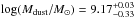 , respectively. Our stellar masses and dust temperatures are similar to those of the 870 μm selected ALESS SMGs that are equally bright as our AzTEC SMGs (da Cunha et al. 2015), while the other parameter values for our SMGs are ~ 1.5−2 times higher on average. Given the spread of the values (the 16th–84th percentile ranges), however, the latter discrepancies are not statistically signifcant. Nevertheless, part of this discrepancy is potentially caused by the different observed wavelengths of the two SMG samples (i.e. λobs = 1.1 mm versus λobs = 870μm).
 -
2.
When compared with the galaxy main sequence as defined by Speagle et al. (2014), our SMGs lie by a factor of
 to
to  above the main sequence. The median SFR/SFRMS ratio is found to be , and most (63%) of the target SMGs can be considered starbursts.
 -
3.
The 3 GHz radio sizes of our SMGs measured in Paper II were used in conjunction with the present stellar mass values to examine their possible stellar mass-size relationship. In particular, the radio sizes of the z> 3 SMGs appear fairly consistent with the z ~ 2 cQGs’ mass–size relation, supporting a scenario where the high-redshift SMGs experience a cQG phase at z ~ 2 (Toft et al. 2014).
-
4.
We used 325 MHz GMRT data in conjuction with the 1.4 GHz and 3 GHz VLA data to investigate the radio SED properties of our SMGs. A radio SED could be constructed for 19 SMGs in total, where each source was detected at least in one of the aforementioned radio bands. The median radio spectral index measured between the observed frame 325 MHz and 3 GHz was found to be
 , which is consistent with the canonical radio synchrotron value (α ≃ −0.8...−0.7).
 -
5.
We found evidence of both spectral flattening and steepening in the radio SEDs of our SMGs, which are indicative of different cosmic-ray energy gain and loss mechanisms taking place in these sources. In the case of the zphot ≃ 1.8 SMG AzTEC 4, which shows the flattest radio spectral index derived here (α> −0.18), the flattening could be due to a non-negligible contribution of thermal free-free emission, which is estimated to be at least one-third of the observed-frame 3 GHz flux density for this source.
-
6.
We found an indication for an anti-correlation between the distance from the galaxy main sequence and 3 GHz radio size. This suggests that starburst SMGs are more compact and hence more susceptible to free-free absorption.
-
7.
The present data allowed us to study the IR-radio correlation among our SMGs. This was quantified by calculating the total-IR q parameter, and its median value was determined to be
. This is in very good agreement with the median q parameter of 2.29 ± 0.09 (recalculated from Thomson et al. 2014) of the flux-limited (i.e. equally bright) ALESS SMGs. We found a statistically insignificant hint of negative correlation between the q parameter and the source redshift in the binned average data. The weakness of this q evolution might be partially caused by the selection effect of our SMGs being essentially IR-selected, but not necessarily detected at the rest-frame 1.4 GHz used to calculate q. This can bias the q parameter towards higher values, and flatten the q(z) distribution. Some of the observed low and high q values compared to the local median value could be linked to the source evolutionary phase. -
8.
The two high redshift SMGs in our sample (AzTEC 1 and AzTEC 3), which benefit from previous CO line data were analysed in further detail (see Appendix D). These SMGs are found to form stars near or at the Eddington limit, where the process of star formation can exhaust the gas reservoir in only
and Myr, respectively. The current stellar and gas mass estimates for AzTEC 1 and 3 suggest they can both evolve to have a final stellar mass of > 1011M⊙. Overall, the results of our study support the general view that high-z (z ≳ 3) SMGs are the progenitors of the present-day giant, gas-poor ellipticals, mostly sitting in the cores of galaxy clusters.
The data products are produced by TERAPIX; see http://terapix.iap.fr
Herschel is an ESA space observatory with science instruments provided by European-led Principal Investigator consortia and with important participation from NASA.
MAGPHYS is publicly available and can be retrieved at http://www.iap.fr/magphys/magphys/MAGPHYS.html
https://cran.r-project.org/web/packages/dblcens/
Acknowledgments
We would like to thank the anonymous referee for pro- viding us with comments and suggestions. This research was funded by the European Union’s Seventh Framework programme under grant agreement 337595 (ERC Starting Grant, “CoSMass”). This work was completed at the Aspen Center for Physics, which is supported by National Science Foundation grant PHY-1066293. This work was partially supported by a grant from the Simons Foundation. M.A. acknowledges partial support from FONDE-CYT through grant 1140099. A.K. acknowledges support by the Collaborative Research Council 956, sub-project A1, funded by the Deutsche Forschungsgemeinschaft (DFG). This paper makes use of the following ALMA data: ADS/JAO.ALMA#2012.1.00978.S and ADS/JAO.ALMA#2013.1.00118.S. ALMA is a partnership of ESO (representing its member states), NSF (USA) and NINS (Japan), together with NRC (Canada), NSC and ASIAA (Taiwan), and KASI (Republic of Korea), in cooperation with the Republic of Chile. The Joint ALMA Observatory is operated by ESO, AUI/NRAO, and NAOJ. This paper is also partly based on data products from observations made with ESO Telescopes at the La Silla Paranal Observatory under ESO programme ID 179.A-2005 and on data products produced by TERAPIX and the Cambridge Astronomy Survey Unit on behalf of the UltraVISTA consortium. This research has made use of NASA’s Astrophysics Data System, and the NASA/IPAC Infrared Science Archive, which is operated by the JPL, California Institute of Technology, under contract with the NASA. We greatfully acknowledge the contributions of the entire COSMOS collaboration consisting of more than 100 scientists. More information on the COSMOS survey is available at http://cosmos.astro.caltech.edu.
PACS has been developed by a consortium of institutes led by MPE (Germany) and including UVIE (Austria); KU Leuven, CSL, IMEC (Belgium); CEA, LAM (France); MPIA (Germany); INAF-IFSI/OAA/OAP/OAT, LENS, SISSA (Italy); IAC (Spain). This development has been supported by the funding agencies BMVIT (Austria), ESA-PRODEX (Belgium), CEA/CNES (France), DLR (Germany), ASI/INAF (Italy), and CICYT/MCYT (Spain).
SPIRE has been developed by a consortium of institutes led by Cardiff University (UK) and including Univ. Lethbridge (Canada); NAOC (China); CEA, LAM (France); IFSI, Univ. Padua (Italy); IAC (Spain); Stockholm Observatory (Sweden); Imperial College London, RAL, UCL-MSSL, UKATC, Univ. Sussex (UK); and Caltech, JPL, NHSC, Univ. Colorado (USA). This development has been supported by national funding agencies: CSA (Canada); NAOC (China); CEA, CNES, CNRS (France); ASI (Italy); MCINN (Spain); SNSB (Sweden); STFC, UKSA (UK); and NASA (USA).
References
- Alaghband-Zadeh, S., Chapman, S. C., Swinbank, A. M., et al. 2012, MNRAS, 424, 2232 [NASA ADS] [CrossRef] [Google Scholar]
- Andrews, B. H., & Thompson, T. A. 2011, ApJ, 727, 97 [NASA ADS] [CrossRef] [Google Scholar]
- Aretxaga, I., Wilson, G. W., Aguilar, E., et al. 2011, MNRAS, 415, 3831 [NASA ADS] [CrossRef] [Google Scholar]
- Barger, A. J., Cowie, L. L., Sanders, D. B., et al. 1998, Nature, 394, 248 [NASA ADS] [CrossRef] [Google Scholar]
- Barger, A. J., Wang, W.-H., Cowie, L. L., et al. 2012, ApJ, 761, 89 [Google Scholar]
- Basu, A., Beck, R., Schmidt, P., & Roy, S. 2015, MNRAS, 449, 3879 [NASA ADS] [CrossRef] [Google Scholar]
- Bell, E. F. 2003, ApJ, 586, 794 [Google Scholar]
- Belli, S., Newman, A. B., & Ellis, R. S. 2014, ApJ, 783, 117 [NASA ADS] [CrossRef] [Google Scholar]
- Berta, S., Lutz, D., Santini, P., et al. 2013, A&A, 551, A100 [NASA ADS] [CrossRef] [EDP Sciences] [Google Scholar]
- Béthermin, M., De Breuck, C., Sargent, M., & Daddi, E. 2015, A&A, 576, L9 [NASA ADS] [CrossRef] [EDP Sciences] [Google Scholar]
- Bolzonella, M., Miralles, J.-M., & Pelló, R. 2000, A&A, 363, 476 [NASA ADS] [Google Scholar]
- Boulade, O., Charlot, X., Abbon, P., et al. 2003, Proc. SPIE, 4841, 72 [NASA ADS] [CrossRef] [Google Scholar]
- Bressan, A., Silva, L., & Granato, G. L. 2002, A&A, 392, 377 [NASA ADS] [CrossRef] [EDP Sciences] [Google Scholar]
- Brinchmann, J., Charlot, S., White, S. D. M., et al. 2004, MNRAS, 351, 1151 [NASA ADS] [CrossRef] [Google Scholar]
- Bruzual, G. 2007, From Stars to Galaxies: Building the Pieces to Build Up the Universe, ASP Conf. Ser., 374, 303 [NASA ADS] [Google Scholar]
- Bruzual, G., & Charlot, S. 2003, MNRAS, 344, 1000 [NASA ADS] [CrossRef] [Google Scholar]
- Capak, P., Aussel, H., Ajiki, M., et al. 2007, ApJS, 172, 99 [NASA ADS] [CrossRef] [Google Scholar]
- Capak, P. L., Riechers, D., Scoville, N. Z., et al. 2011, Nature, 470, 233 [Google Scholar]
- Capak, P. L., Carilli, C., Jones, G., et al. 2015, Nature, 522, 455 [NASA ADS] [CrossRef] [Google Scholar]
- Carilli, C. L., & Yun, M. S. 1999, ApJ, 513, L13 [NASA ADS] [CrossRef] [Google Scholar]
- Carilli, C. L., & Yun, M. S. 2000, ApJ, 530, 618 [NASA ADS] [CrossRef] [Google Scholar]
- Carilli, C. L., & Walter, F. 2013, ARA&A, 51, 105 [NASA ADS] [CrossRef] [EDP Sciences] [Google Scholar]
- Casey, C. M., Berta, S., Béthermin, M., et al. 2012, ApJ, 761, 140 [NASA ADS] [CrossRef] [Google Scholar]
- Casey, C. M., Chen, C.-C., Cowie, L. L., et al. 2013, MNRAS, 436, 1919 [NASA ADS] [CrossRef] [Google Scholar]
- Casey, C. M., Narayanan, D., & Cooray, A. 2014, Phys. Rep., 541, 45 [NASA ADS] [CrossRef] [Google Scholar]
- Chabrier, G. 2003, PASP, 115, 763 [NASA ADS] [CrossRef] [Google Scholar]
- Chapman, S. C., Blain, A. W., Smail, I., & Ivison, R. J. 2005, ApJ, 622, 772 [NASA ADS] [CrossRef] [Google Scholar]
- Condon, J. J. 1992, ARA&A, 30, 575 [NASA ADS] [CrossRef] [MathSciNet] [Google Scholar]
- Condon, J. J., Anderson, M. L., & Helou, G. 1991, ApJ, 376, 95 [NASA ADS] [CrossRef] [Google Scholar]
- da Cunha, E., Charlot, S., & Elbaz, D. 2008, MNRAS, 388, 1595 [NASA ADS] [CrossRef] [Google Scholar]
- da Cunha, E., Charmandaris, V., Díaz-Santos, T., et al. 2010, A&A, 523, A78 [NASA ADS] [CrossRef] [EDP Sciences] [Google Scholar]
- da Cunha, E., Walter, F., Smail, I., et al. 2015, ApJ, 806, 110 [NASA ADS] [CrossRef] [Google Scholar]
- Daddi, E., Dickinson, M., Morrison, G., et al. 2007, ApJ, 670, 156 [NASA ADS] [CrossRef] [Google Scholar]
- Daddi, E., Dannerbauer, H., Stern, D., et al. 2009, ApJ, 694, 1517 [Google Scholar]
- Dale, D. A., & Helou, G. 2002, ApJ, 576, 159 [NASA ADS] [CrossRef] [Google Scholar]
- De Breuck, C., Maiolino, R., Caselli, P., et al. 2011, A&A, 530, L8 [NASA ADS] [CrossRef] [EDP Sciences] [Google Scholar]
- de Jong, T., Klein, U., Wielebinski, R., & Wunderlich, E. 1985, A&A, 147, L6 [NASA ADS] [Google Scholar]
- Dekel, A., Birnboim, Y., Engel, G., et al. 2009, Nature, 457, 451 [NASA ADS] [CrossRef] [PubMed] [Google Scholar]
- DelMoro, A., Alexander, D. M., Mullaney, J. R., et al. 2013, A&A, 549, A59 [NASA ADS] [CrossRef] [EDP Sciences] [Google Scholar]
- Delhaize, J., Smolčić, V., Delvecchio, I., et al. 2016, A&A, submitted [Google Scholar]
- Dessauges-Zavadsky, M., Zamojski, M., Schaerer, D., et al. 2015, A&A, 577, A50 [NASA ADS] [CrossRef] [EDP Sciences] [Google Scholar]
- Draine, B. T., & Li, A. 2007, ApJ, 657, 810 [NASA ADS] [CrossRef] [Google Scholar]
- Dwek, E., Staguhn, J. G., Arendt, R. G., et al. 2011, ApJ, 738, 36 [NASA ADS] [CrossRef] [Google Scholar]
- Dye, S., Eales, S. A., Aretxaga, I., et al. 2008, MNRAS, 386, 1107 [NASA ADS] [CrossRef] [Google Scholar]
- Eales, S., Lilly, S., Gear, W., et al. 1999, ApJ, 515, 518 [NASA ADS] [CrossRef] [Google Scholar]
- Efstathiou, A., Rowan-Robinson, M., & Siebenmorgen, R. 2000, MNRAS, 313, 734 [NASA ADS] [CrossRef] [Google Scholar]
- Elbaz, D., Daddi, E., Le Borgne, D., et al. 2007, A&A, 468, 33 [NASA ADS] [CrossRef] [EDP Sciences] [Google Scholar]
- Engel, H., Tacconi, L. J., Davies, R. I., et al. 2010, ApJ, 724, 233 [NASA ADS] [CrossRef] [Google Scholar]
- Fazio, G. G., Hora, J. L., Allen, L. E., et al. 2004, ApJS, 154, 10 [NASA ADS] [CrossRef] [Google Scholar]
- Fu, H., Cooray, A., Feruglio, C., et al. 2013, Nature, 498, 338 [NASA ADS] [CrossRef] [Google Scholar]
- Genzel, R., Tacconi, L. J., Combes, F., et al. 2012, ApJ, 746, 69 [NASA ADS] [CrossRef] [Google Scholar]
- Hayward, C. C., & Smith, D. J. B. 2015, MNRAS, 446, 1512 [NASA ADS] [CrossRef] [Google Scholar]
- Hayward, C. C., Kereš, D., Jonsson, P., et al. 2011, ApJ, 743, 159 [CrossRef] [Google Scholar]
- Hayward, C. C., Jonsson, P., Kereš, D., et al. 2012, MNRAS, 424, 951 [NASA ADS] [CrossRef] [Google Scholar]
- Helou, G., Soifer, B. T., & Rowan-Robinson, M. 1985, ApJ, 298, L7 [Google Scholar]
- Helsel, D. R. 2005, Nondetects And Data Analysis: Statistics for Censored Environmental Data (New York: John Wiley and Sons) [Google Scholar]
- Hodge, J. A., Karim, A., Smail, I., et al. 2013, ApJ, 768, 91 [NASA ADS] [CrossRef] [Google Scholar]
- Huang, J.-S., Rigopoulou, D., Magdis, G., et al. 2014, ApJ, 784, 52 [NASA ADS] [CrossRef] [Google Scholar]
- Hughes, D. H., Serjeant, S., Dunlop, J., et al. 1998, Nature, 394, 241 [NASA ADS] [CrossRef] [Google Scholar]
- Ilbert, O., Capak, P., Salvato, M., et al. 2009, ApJ, 690, 1236 [NASA ADS] [CrossRef] [Google Scholar]
- Ilbert, O., McCracken, H. J., Le Fèvre, O., et al. 2013, A&A, 556, A55 [NASA ADS] [CrossRef] [EDP Sciences] [Google Scholar]
- Ivison, R. J., Alexander, D. M., Biggs, A. D., et al. 2010a, MNRAS, 402, 245 [NASA ADS] [CrossRef] [Google Scholar]
- Ivison, R. J., Magnelli, B., Ibar, E., et al. 2010b, A&A, 518, L31 [NASA ADS] [CrossRef] [EDP Sciences] [Google Scholar]
- Karim, A., Schinnerer, E., Martínez-Sansigre, A., et al. 2011, ApJ, 730, 61 [NASA ADS] [CrossRef] [Google Scholar]
- Karim, A., Swinbank, A. M., Hodge, J. A., et al. 2013, MNRAS, 432, 2 [NASA ADS] [CrossRef] [Google Scholar]
- Kennicutt, R. C., Jr. 1998, ApJ, 498, 541 [NASA ADS] [CrossRef] [Google Scholar]
- Koprowski, M. P., Dunlop, J. S., Michałowski, M. J., et al. 2014, MNRAS, 444, 117 [NASA ADS] [CrossRef] [Google Scholar]
- Koprowski, M. P., Dunlop, J. S., Michałowski, M. J., et al. 2016, MNRAS, 458, 4321 [NASA ADS] [CrossRef] [Google Scholar]
- Kovács, A., Chapman, S. C., Dowell, C. D., et al. 2006, ApJ, 650, 592 [NASA ADS] [CrossRef] [Google Scholar]
- Krogager, J.-K., Zirm, A. W., Toft, S., et al. 2014, ApJ, 797, 17 [NASA ADS] [CrossRef] [Google Scholar]
- Laigle, C., McCracken, H. J., Ilbert, O., et al. 2016, ApJS, 224, 24 [NASA ADS] [CrossRef] [Google Scholar]
- Leroy, A. K., Bolatto, A., Gordon, K., et al. 2011, ApJ, 737, 12 [NASA ADS] [CrossRef] [Google Scholar]
- Lisenfeld, U., & Völk, H. J. 2000, A&A, 354, 423 [NASA ADS] [Google Scholar]
- Lupton, R. 1993, Statistics in Theory and Practice (Princeton University Press) [Google Scholar]
- Lutz, D., Poglitsch, A., Altieri, B., et al. 2011, A&A, 532, A90 [NASA ADS] [CrossRef] [EDP Sciences] [Google Scholar]
- Magdis, G. E., Daddi, E., Béthermin, M., et al. 2012, ApJ, 760, 6 [NASA ADS] [CrossRef] [Google Scholar]
- Magnelli, B., Lutz, D., Berta, S., et al. 2010, A&A, 518, L28 [NASA ADS] [CrossRef] [EDP Sciences] [Google Scholar]
- Magnelli, B., Lutz, D., Santini, P., et al. 2012, A&A, 539, A155 [NASA ADS] [CrossRef] [EDP Sciences] [Google Scholar]
- Magnelli, B., Ivison, R. J., Lutz, D., et al. 2015, A&A, 573, A45 [NASA ADS] [CrossRef] [EDP Sciences] [Google Scholar]
- Marvil, J., Owen, F., & Eilek, J. 2015, AJ, 149, 32 [NASA ADS] [CrossRef] [Google Scholar]
- McCracken, H. J., Capak, P., Salvato, M., et al. 2010, ApJ, 708, 202 [NASA ADS] [CrossRef] [Google Scholar]
- McCracken, H. J., Milvang-Jensen, B., Dunlop, J., et al. 2012, A&A, 544, A156 [NASA ADS] [CrossRef] [EDP Sciences] [Google Scholar]
- Michałowski, M. J., Dunlop, J. S., Cirasuolo, M., et al. 2012, A&A, 541, A85 [NASA ADS] [CrossRef] [EDP Sciences] [Google Scholar]
- Michałowski, M. J., Hayward, C. C., Dunlop, J. S., et al. 2014, A&A, 571, A75 [NASA ADS] [CrossRef] [EDP Sciences] [Google Scholar]
- Miettinen, O., Smolčić, V., Novak, M., et al. 2015a, A&A, 577, A29 (Paper I) [NASA ADS] [CrossRef] [EDP Sciences] [Google Scholar]
- Miettinen, O., Novak, M., Smolčić, V., et al. 2015b, A&A, 584, A32 (Paper II) [NASA ADS] [CrossRef] [EDP Sciences] [Google Scholar]
- Miller, N. A., & Owen, F. N. 2001, AJ, 121, 1903 [NASA ADS] [CrossRef] [Google Scholar]
- Miyazaki, S., Komiyama, Y., Sekiguchi, M., et al. 2002, PASJ, 54, 833 [NASA ADS] [CrossRef] [Google Scholar]
- Miyazaki, S., Komiyama, Y., Nakaya, H., et al. 2012, Proc. SPIE, 8446, 84460 [Google Scholar]
- Murphy, E. J. 2009, ApJ, 706, 482 [NASA ADS] [CrossRef] [Google Scholar]
- Murphy, E. J., Kenney, J. D. P., Helou, G., Chung, A., & Howell, J. H. 2009, ApJ, 694, 1435 [NASA ADS] [CrossRef] [Google Scholar]
- Murphy, E. J., Helou, G., Condon, J. J., et al. 2010, ApJ, 709, L108 [NASA ADS] [CrossRef] [Google Scholar]
- Murphy, E. J., Condon, J. J., Schinnerer, E., et al. 2011, ApJ, 737, 67 [NASA ADS] [CrossRef] [Google Scholar]
- Murphy, E. J., Stierwalt, S., Armus, L., et al. 2013, ApJ, 768, 2 [NASA ADS] [CrossRef] [Google Scholar]
- Narayanan, D., Cox, T. J., Hayward, C. C., et al. 2009, MNRAS, 400, 1919 [NASA ADS] [CrossRef] [MathSciNet] [Google Scholar]
- Narayanan, D., Turk, M., Feldmann, R., et al. 2015, Nature, 525, 496 [NASA ADS] [CrossRef] [PubMed] [Google Scholar]
- Niklas, S., Klein, U., & Wielebinski, R. 1997, A&A, 322, 19 [NASA ADS] [Google Scholar]
- Noeske, K. G., Weiner, B. J., Faber, S. M., et al. 2007, ApJ, 660, L43 [Google Scholar]
- Oliver, S. J., Bock, J., Altieri, B., et al. 2012, MNRAS, 424, 1614 [NASA ADS] [CrossRef] [EDP Sciences] [Google Scholar]
- Puget, P., Stadler, E., Doyon, R., et al. 2004, Proc. SPIE, 5492, 978 [Google Scholar]
- Reddy, N. A., & Yun, M. S. 2004, ApJ, 600, 695 [NASA ADS] [CrossRef] [Google Scholar]
- Renzini, A., & Peng, Y.-j. 2015, ApJ, 801, L29 [NASA ADS] [CrossRef] [Google Scholar]
- Riechers, D. A., Capak, P. L., Carilli, C. L., et al. 2010, ApJ, 720, L131 [NASA ADS] [CrossRef] [Google Scholar]
- Riechers, D. A., Bradford, C. M., Clements, D. L., et al. 2013, Nature, 496, 329 [Google Scholar]
- Riechers, D. A., Carilli, C. L., Capak, P. L., et al. 2014, ApJ, 796, 84 [NASA ADS] [CrossRef] [Google Scholar]
- Rieke, G. H., Young, E. T., Engelbracht, C. W., et al. 2004, ApJS, 154, 25 [NASA ADS] [CrossRef] [Google Scholar]
- Roseboom, I. G., Dunlop, J. S., Cirasuolo, M., et al. 2013, MNRAS, 436, 430 [NASA ADS] [CrossRef] [Google Scholar]
- Roussel, H., Helou, G., Beck, R., et al. 2003, ApJ, 593, 733 [Google Scholar]
- Rowlands, K., Dunne, L., Dye, S., et al. 2014a, MNRAS, 441, 1017 [NASA ADS] [CrossRef] [Google Scholar]
- Rowlands, K., Gomez, H. L., Dunne, L., et al. 2014b, MNRAS, 441, 1040 [NASA ADS] [CrossRef] [MathSciNet] [Google Scholar]
- Salmon, B., Papovich, C., Finkelstein, S. L., et al. 2015, ApJ, 799, 183 [NASA ADS] [CrossRef] [Google Scholar]
- Sanders, D. B., Salvato, M., Aussel, H., et al. 2007, ApJS, 172, 86 [Google Scholar]
- Sargent, M. T., Schinnerer, E., Murphy, E., et al. 2010, ApJ, 714, L190 [NASA ADS] [CrossRef] [Google Scholar]
- Schinnerer, E., Smolčić, V., Carilli, C. L., et al. 2007, ApJS, 172, 46 [NASA ADS] [CrossRef] [Google Scholar]
- Schinnerer, E., Carilli, C. L., Capak, P., et al. 2008, ApJ, 689, L5 [Google Scholar]
- Schinnerer, E., Sargent, M. T., Bondi, M., et al. 2010, ApJS, 188, 384 [NASA ADS] [CrossRef] [Google Scholar]
- Schleicher, D. R. G., & Beck, R. 2013, A&A, 556, A142 [NASA ADS] [CrossRef] [EDP Sciences] [Google Scholar]
- Schober, J., Schleicher, D. R. G., & Klessen, R. S. 2016, ApJ, 827, 109 [NASA ADS] [CrossRef] [Google Scholar]
- Scott, K. S., Austermann, J. E., Perera, T. A., et al. 2008, MNRAS, 385, 2225 [NASA ADS] [CrossRef] [Google Scholar]
- Scoville, N. 2003, J. Korean Astron. Soc., 36, 167 [NASA ADS] [CrossRef] [Google Scholar]
- Scoville, N. 2004, The Neutral ISM in Starburst Galaxies, ASP Conf. Ser., 320, 253 [NASA ADS] [Google Scholar]
- Scoville, N., Aussel, H., Brusa, M., et al. 2007, ApJS, 172, 1 [NASA ADS] [CrossRef] [Google Scholar]
- Seymour, N., Altieri, B., De Breuck, C., et al. 2012, ApJ, 755, 146 [NASA ADS] [CrossRef] [Google Scholar]
- Silva, L., Granato, G. L., Bressan, A., & Danese, L. 1998, ApJ, 509, 103 [NASA ADS] [CrossRef] [Google Scholar]
- Simpson, J. M., Swinbank, A. M., Smail, I., et al. 2014, ApJ, 788, 125 [Google Scholar]
- Simpson, J. M., Smail, I., Swinbank, A. M., et al. 2015, ApJ, 807, 128 [NASA ADS] [CrossRef] [Google Scholar]
- Smail, I., Ivison, R. J., & Blain, A. W. 1997, ApJ, 490, L5 [NASA ADS] [CrossRef] [Google Scholar]
- Smith, D. J. B., Dunne, L., da Cunha, E., et al. 2012, MNRAS, 427, 703 [NASA ADS] [CrossRef] [Google Scholar]
- Smolčić, V., Capak, P., Ilbert, O., et al. 2011, ApJ, 731, L27 [NASA ADS] [CrossRef] [Google Scholar]
- Smolčić, V., Aravena, M., Navarrete, F., et al. 2012, A&A, 548, A4 [NASA ADS] [CrossRef] [EDP Sciences] [Google Scholar]
- Smolčić, V., Karim, A., Miettinen, O., et al. 2015, A&A, 576, A127 [NASA ADS] [CrossRef] [EDP Sciences] [Google Scholar]
- Smolčić, V., Miettinen, O., Tomičić, N., et al. 2016a, A&A, 597, A4 (Paper III) [NASA ADS] [Google Scholar]
- Smolčić, V., Novak, M., Bondi, M., et al. 2016b, A&A, in press, DOI: 10.1051/0004-6361/201628704 [Google Scholar]
- Socrates, A., Davis, S. W., & Ramirez-Ruiz, E. 2008, ApJ, 687, 202 [NASA ADS] [CrossRef] [Google Scholar]
- Speagle, J. S., Steinhardt, C. L., Capak, P. L., & Silverman, J. D. 2014, ApJS, 214, 15 [NASA ADS] [CrossRef] [Google Scholar]
- Steinhardt, C. L., Speagle, J. S., Capak, P., et al. 2014, ApJ, 791, LL25 [NASA ADS] [CrossRef] [Google Scholar]
- Strandet, M. L., Weiß, A., Vieira, J. D., et al. 2016, ApJ, 822, 80 [NASA ADS] [CrossRef] [Google Scholar]
- Swinbank, A. M., Chapman, S. C., Smail, I., et al. 2006, MNRAS, 371, 465 [NASA ADS] [CrossRef] [Google Scholar]
- Swinbank, A. M., Karim, A., Smail, I., et al. 2012, MNRAS, 427, 1066 [NASA ADS] [CrossRef] [Google Scholar]
- Swinbank, A. M., Simpson, J. M., Smail, I., et al. 2014, MNRAS, 438, 1267 [Google Scholar]
- Tacconi, L. J., Genzel, R., Smail, I., et al. 2008, ApJ, 680, 246 [NASA ADS] [CrossRef] [PubMed] [Google Scholar]
- Tan, Q., Daddi, E., Magdis, G., et al. 2014, A&A, 569, A98 [NASA ADS] [CrossRef] [EDP Sciences] [Google Scholar]
- Taniguchi, Y., Scoville, N., Murayama, T., et al. 2007, ApJS, 172, 9 [NASA ADS] [CrossRef] [Google Scholar]
- Taniguchi, Y., Kajisawa, M., Kobayashi, M. A. R., et al. 2015, PASJ, 67, 104 [NASA ADS] [Google Scholar]
- Thompson, T. A., Quataert, E., & Murray, N. 2005, ApJ, 630, 167 [NASA ADS] [CrossRef] [Google Scholar]
- Thompson, T. A., Quataert, E., Waxman, E., Murray, N., & Martin, C. L. 2006, ApJ, 645, 186 [NASA ADS] [CrossRef] [Google Scholar]
- Thomson, A. P., Ivison, R. J., Simpson, J. M., et al. 2014, MNRAS, 442, 577 [NASA ADS] [CrossRef] [Google Scholar]
- Thomson, A. P., Ivison, R. J., Owen, F. N., et al. 2015, MNRAS, 448, 1874 [NASA ADS] [CrossRef] [Google Scholar]
- Toft, S., Smolčić, V., Magnelli, B., et al. 2014, ApJ, 782, 68 [NASA ADS] [CrossRef] [Google Scholar]
- van der Kruit, P. C. 1971, A&A, 15, 110 [NASA ADS] [Google Scholar]
- Weiß, A., Kovács, A., Coppin, K., et al. 2009, ApJ, 707, 1201 [NASA ADS] [CrossRef] [Google Scholar]
- Whitaker, K. E., van Dokkum, P. G., Brammer, G., & Franx, M. 2012, ApJ, 754, L29 [NASA ADS] [CrossRef] [Google Scholar]
- Whitaker, K. E., van Dokkum, P. G., Brammer, G., et al. 2013, ApJ, 770, L39 [NASA ADS] [CrossRef] [Google Scholar]
- Wiklind, T., Conselice, C. J., Dahlen, T., et al. 2014, ApJ, 785, 111 [NASA ADS] [CrossRef] [Google Scholar]
- Yang, M., Greve, T. R., Dowell, C. D., & Borys, C. 2007, ApJ, 660, 1198 [NASA ADS] [CrossRef] [Google Scholar]
- Younger, J. D., Fazio, G. G., Huang, J.-S., et al. 2007, ApJ, 671, 1531 [Google Scholar]
- Younger, J. D., Fazio, G. G., Wilner, D. J., et al. 2008, ApJ, 688, 59 [NASA ADS] [CrossRef] [Google Scholar]
- Younger, J. D., Fazio, G. G., Huang, J.-S., et al. 2009, ApJ, 704, 803 [NASA ADS] [CrossRef] [Google Scholar]
- Younger, J. D., Fazio, G. G., Ashby, M. L. N., et al. 2010, MNRAS, 407, 1268 [NASA ADS] [CrossRef] [Google Scholar]
- Yuan, F., Buat, V., Burgarella, D., et al. 2015, A&A, 582, A90 [NASA ADS] [CrossRef] [EDP Sciences] [Google Scholar]
- Yun, M. S., Reddy, N. A., & Condon, J. J. 2001, ApJ, 554, 803 [NASA ADS] [CrossRef] [Google Scholar]
- Yun, M. S., Aretxaga, I., Gurwell, M. A., et al. 2015, MNRAS, 454, 3485 [NASA ADS] [CrossRef] [Google Scholar]
Appendix A: Photometric tables
A selection of mid-IR to mm flux densities of our SMGs are listed in Table A.1. The GMRT (325 MHz) and VLA (1.4 and 3 GHz) radio flux densities are tabulated in Table A.2.
Flux densities at mid-IR to mm wavelengths in mJy.
Flux densities of our SMGs at the observed radio frequencies of 325 MHz, 1.4 GHz, and 3 GHz.
Appendix B: Revised redshifts, unsatisfying SED model fits, and a revisit of the sample statistics
Appendix B.1: Revised redshifts
AzTEC 17a was previously thought to lie at a spectroscopic redshift of zspec = 0.834 (see Paper I, and references therein) and, hence, to be the lowest-redshift SMG in our sample. However, the source SED, which was constructed assuming this redshift, showed that the Herschel flux density upper limits were inconsistent with the best-fit SED model; this suggests that the redshift was underestimated.
The different redshift estimates for AzTEC 17a were discussed in Appendix C of Paper I. A spec-z of zspec = 0.834 for AzTEC 17a is reported to be very secure in the COSMOS spec-z catalogue (M. Salvato et al., in prep.), but our initial SED fit suggested that the SMG redshift is higher. Here, we have adopted a redshift of  reported in the COSMOS2015 catalogue (Laigle et al. 2016) for the source ID835094, which lies
  away from the PdBI 1.3 mm peak position of AzTEC 17a. We note that, although it is lying outside the area covered by the slit used for the spectroscopic measurements towards AzTEC 17a, there is a galaxy (ID836198) lying
  NW of the PdBI 1.3 mm peak of AzTEC 17a (see Fig. E.1 in Paper I). A likely zspec value of zspec = 0.78792 (quality flag 2) is reported for this galaxy in the COSMOS spec-z catalogue (M. Salvato et al., in prep.), while the COSMOS2015 catalogue (Laigle et al. 2016) gives a photo-z value of
  , in fairly good agreement with the corresponding spec-z. Hence, it seems possible that the spectroscopic redshift measurement towards AzTEC 17a was contaminated by radiation from this foreground galaxy.
Moreover, the redshifts of AzTEC 4, 5, 9, 12, 15, and 24b were recomputed using the COSMOS2015 photometric catalogue (Laigle et al. 2016) as part of the redshift distribution analysis of the ALMA-detected ASTE/AzTEC SMGs (D. Brisbin et al., in prep.).
For AzTEC 4, the nominal value of the updated redshift of  is much lower than the previous estimate (
 ; Smolčić et al. 2012), but the photometric redshift of this source suffers from very large uncertainties.
In the case of AzTEC 5, the updated redshift of  is consistent with the previous value within the uncertainties (
 ; Smolčić et al. 2012; see also Paper I).
For AzTEC 9, we derived a new photometric redshift of  . A spec-z of zspec = 1.357 has been measured for AzTEC 9, but it is based on a relatively weak spectrum (M. Salvato et al., in prep.), and is therefore uncertain. Nevertheless, this spec-z is comparable to a photo-z of
  previously derived for AzTEC 9 by Smolčić et al. (2012). Also, the COSMOS2015 catalogue (Laigle et al. 2016) gives a secondary photo-z solution of zphot = 4.55 for a source lying
  from AzTEC 9 (ID763214). Moreover, Koprowski et al. (2014) derived a redshift of
  , which was based on a K-band counterpart lying
  away from the SMA 890 μm position of AzTEC 9. The latter two redshifts are comparable to our new value.
The updated photometric redshift that we obtained for AzTEC 12,  , is slightly higher than the previous value of
  from Smolčić et al. (2012).
For AzTEC 15, the updated redshift of  is somewhat lower than the previous estimate (
 ; Smolčić et al. 2012), but the large associated uncertainties make the two consistent with each other.
Finally, for AzTEC 24b, we computed a redshift of  on the basis of a new counterpart identification enabled by our new ALMA data (cf. Paper I). Our PdBI 1.3 mm source AzTEC 24b lies
  NE of a 1.3 mm detected ALMA SMG (M. Aravena et al., in prep.). We can attribute this nominally large offset to the poorer quality of the PdBI data than the corresponding ALMA data.
Appendix B.2: Spectral energy distribution fits of other sources
In Fig. B.1, we show the SED fits for AzTEC 2, 6, 11-N, 19b, and 26a. In the case of AzTEC 2, the lack of UV/optical to NIR data does not allow a meaningful MAGPHYS fit, and hence the derived properties, such as the stellar mass, could not be constrained. Moreover, AzTEC 2 might lie at a higher redshift than zspec = 1.125 because it is found to be the brightest 2 mm source in the IRAM/GISMO (Institut de Radioastronomie Millimétrique/Goddard-IRAM Superconducting 2 Millimetre Observer) 2 mm survey of the COSMOS field (A. Karim et al., in prep.), and it is possibly affected by galaxy-galaxy lensing. As discussed in Paper I (Appendix B therein), the redshift of AzTEC 6 is also uncertain. As shown in Fig. B.1, the assumption that the SMG lies at zspec = 0.802 does not yield a satisfying SED fit, but it rather suggests a higher redshift (cf. AzTEC 17a). Indeed, a non-detection of AzTEC 6 at 1.4 GHz suggests a redshift of z> 3.52 (Paper I). For AzTEC 11-N, the optical to NIR photometry was manually extracted from the ALMA 1.3 mm peak position owing to the nearby source AzTEC 11-S. However, no reasonable SED fit could be obtained for this source. The derived SED fits for AzTEC 19b and 26a are also poor. Given that AzTEC 19b was identified at the border of the PdBI primary beam, and the counterpart of AzTEC 26a lies  away from the PdBI emission peak (Paper I), these sources are potentially spurious.
Appendix B.3: Revised SMG sample statistics
Given the aforementioned revised properties of our SMGs, and the fact that two more SMG candidates from our PdBI 1.3 mm survey (Paper I; AzTEC 24a and 24c) were not detected at 1.3 mm with ALMA (M. Aravena et al., in prep.), and are hence very likely to be spurious, we are now in a position where we can revise the statistical properties of our sample. Of the 30 single-dish detected sources
AzTEC 1–30, only up to 5 appear to be resolved into multiple components at an angular resolution of about 2″ (AzTEC 29 being an uncertain case; Paper I). This suggests a revised multiplicity fraction of ~ 17% ± 7% among our target SMGs. The revised sample mean and median redshifts are z = 3.19 ± 0.21 and 3.00 ± 0.26, respectively; these redshifts are consistent with those reported in Paper I (3.19 ± 0.22 and 3.17 ± 0.27). The fraction of 3 GHz detected SMGs in our sample is revised to be 51% ± 12% (cf. Paper II). Assuming the new redshift values for some of our SMGs, the median 3 GHz major axis FWHM is derived to be 4.2 ± 1.1 kpc (4.1 ± 1.0 kpc) for the cosmology adopted therein (in the present work), which is the same as reported in Paper II (4.2 ± 0.9 kpc).
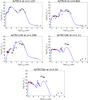 |
Fig. B.1 Best-fit panchromatic (UV-radio) rest-frame SEDs of five of our target SMGs. The source ID and redshift are shown on top of each panel. The red points with vertical error bars represent the observed photometric data, while those with downwards pointing arrows indicate the 3σ upper flux density limits. The blue line is the best-fit MAGPHYS model SED from the high-z library. |
Appendix C: Comparison with previous studies of the physical properties of the JCMT/AzTEC 1.1 mm selected COSMOS SMGs
The SEDs of many of our SMGs have been previously analysed to study their physical properties by Smolčić et al. (2012; AzTEC 1), Magnelli et al. (2012; AzTEC 2, 3, 5, 11-N, and 17a), Casey et al. (2013; AzTEC 2, 5, 9, 19a, 22, 28), Toft et al. (2014; 10 sources among AzTEC 1−15), Huang et al. (2014; AzTEC 1 and 3), Koprowski et al. (2014; 11 sources among AzTEC 1–15), Smolčić et al. (2015; AzTEC 1 and 3), Yuan et al. (2015; AzTEC 1), and Yun et al. (2015; AzTEC 1). We note that only Smolčić et al. (2015) used the MAGPHYS code in their study, although these authors used different priors than we used (see below), and hence a direct comparison with the aforementioned studies is not feasible. Toft et al. (2014) also used MAGPHYS to derive one of the physical parameters of their SMGs, namely the stellar mass. Moreover, Smolčić et al. (2011, 2015), Toft et al. (2014), and Huang et al. (2014) used a redshift of z = 4.64 for AzTEC 1, but its revised spectroscopic redshift is zspec = 4.3415 (Yun et al. 2015). In what follows, we discuss the aforementioned studies in more detail.
Magnelli et al. (2012). While we could not obtain a meaningful MAGPHYS SED for AzTEC 2 and AzTEC 11-N, Magnelli et al. (2012) used a modified blackbody (MBB) fitting method to derive the dust properties of these sources. Out of the five common SMGs to our parent sample, Magnelli et al. (2012) used the same redshift for three sources as we used. The two exceptions are AzTEC 5 and AzTEC 17a, for which they used z = 4.0 and z = 0.8, instead of the values and that we used. We also note that no interferometric (sub)mm observations of AzTEC 17 existed at the time of the study by Magnelli et al. (2012). Based on their single-T MBB fitting (β = 1.5), Magnelli et al. (2012) derived the dust temperature values of Tdust = 53 ± 3 K and 57 ± 4 K for AzTEC 3 and 5, respectively. Within the uncertainties, the Tdust values for AzTEC 3 and 5 are comparable to ours ( and
and  K, respectively) although the values were derived using different methods (and the redshift for AzTEC 5 was slightly different). Our IR luminosities for these two SMGs are about 1.2 and 0.8 times the Magnelli et al. (2012) values, respectively. The dust masses we derived for AzTEC 3 and 5 are 4.2 and 2.8 times higher than the corresponding Magnelli et al. (2012) values. One reason for these discrepancies is probably that Magnelli et al. (2012) did not use the SPIRE 500 μm flux density in their SED analysis. For the above comparisons, we have taken into account the fact that Magnelli et al. (2012) assumed a dust opacity value of κ850 μm = 1.5 cm2 g-1, which is 1.95 times larger than the 850 μm dust opacity of κ850 μm = 0.77 cm2 g-1 adopted in our MAGPHYS analysis.
Casey et al. (2013). These authors used MBB SED fitting combined with a mid-IR power law (see their Eq. (3)). For AzTEC 2 they used a photo-z of  , which is lower than the spec-z of zspec = 1.125 (M. Baloković et al., in prep.). As discussed in Paper I, the aforementioned photo-z refers to the optically visible foreground galaxy seen to the south of AzTEC 2 (see e.g. Fig. E.1 in Paper I). For AzTEC 9, Casey et al. (2013) adopted a redshift of
  , i.e.
  times lower than the value of we derived. For AzTEC 19a, Casey et al. (2013) adopted a redshift of
  , while in Paper I, where we employed the first millimetre interferometric observations towards this source, we derived a photo-z of
  . The SCUBA-2 sources that Casey et al. (2013) detected towards AzTC22 and AzTEC 28, and for which they derived the SEDs, lie
  and
and  away from our PdBI 1.3 mm detections, respectively (Paper I). In Paper I, we found that AzTEC 22 and AzTEC 28 have no optical, IR, or radio counterparts. We do not compare the SED results here for the aforementioned reasons.
Toft et al. (2014). These authors used zspec = 3.971 as the redshift of AzTEC 5. As discussed in Paper I (Appendix B therein), this spec-z is based on a poor quality spectrum, but is still comparable to the revised photo-z of . For AzTEC 11-S, Toft et al. (2014) used a redshift of z> 2.58, but it probably lies at zspec = 1.599 (see Table 1). Although the SEDs of AzTEC 13 and 14-E have not been analysed here, we note that the lower z limits adopted by Toft et al. (2014) for AzTEC 13 (z> 3.59) and 14-E (z> 3.03) are comparable to ours (z> 4.07 and z> 2.95, respectively). Here, we only compare the SED results for AzTEC 3, 5, 8, 10, and 15, in whics the redshifts used were either similar or close to ours. The present stellar masses derived for these SMGs are 0.3 to 1.6 (mean = 0.9, median = 0.6) times those reported by Toft et al. (2014), where the largest discrepancy is found for AzTEC 15, for which the discrepancy in the assumed redshift is the largest (factor of 1.13). The dust masses we derived are lower by factors of 0.2 to 0.8 (mean = 0.5, median = 0.4) than those derived by Toft et al. (2014), who used the physically motivated dust model of Draine & Li (2007) in their analysis. Our IR luminosities are 0.7–1.2 (mean = 0.9, median = 0.9) times the values obtained by Toft et al. (2014), and hence in fairly good agreement. This agreement also applies to the corresponding Kennicutt (1998) SFRs, the authors reported.
Huang et al. (2014). Based on MBB fitting, Huang et al. (2014) derived the values of Tdust = 79 ± 7 K,  M⊙, and
  L⊙ for AzTEC 3 (see their Table 4). The quoted dust mass was scaled up by a factor of 1.06 from the value reported by Huang et al. (2014) to take into account that they adopted a dust opacity of κ250 μm = 5.1 cm2 g-1, while our corresponding value would be 4.8 cm2 g-1 (assuming β = 1.5). Our dust temperature of K for AzTEC 3 is lower than the Huang et al. (2014) value by a factor of
  , which is a reasonable agreement given that they are derived through different methods, and hence not directly comparable. The dust mass we derived is only
  times that obtained by Huang et al. (2014). The IR luminosity from Huang et al. (2014) refers to the FIR range (although the wavelength range was not specified), and our corresponding value of
  L⊙ is
L⊙ is  times their value, and hence in fairly good agreement within the uncertainties. Huang et al. (2014) also derived the qFIR parameter for AzTEC 1 and 3 (but an old redshift value for AzTEC 1 was used as mentioned above). They report the values of qFIR = 2.25 ± 0.29 and qFIR> 2.15, respectively. Our corresponding values for AzTEC 1 and 3 are qFIR = 2.10 ± 0.17 and qFIR = 1.67 ± 0.17, where the AzTEC 1 value is comparable within the uncertainties despite the different redshift used, but for AzTEC 3 the value we derived is inconsistent with the Huang et al. (2014) lower limit.
Koprowski et al. (2014). These authors derived stellar masses for SMGs among AzTEC 1–15 (besides the photo-z values, which was the main purpose of their study; see their Table 5). They used the HYPERZ code (Bolzonella et al. 2000) and assumed a Chabrier (2003) IMF. In all the other cases except AzTEC 4, 5, 7, 10, 12, and 15 the photo-z values derived by the authors are close enough to our adopted redshift values (within a factor of 1.03) that we can make a reasonable comparison between the stellar masses they obtained and those that we derived. The comparison of the stellar masses for AzTEC 1, 3, 8, and 11-S showed that our values are 0.4 to 1.1 (mean = 0.8, median = 0.8) times the values reported by Koprowski et al. (2014), and the average agreement is fairly good.
Smolčić et al. (2015). The most direct comparison we can make is with the MAGPHYS SED of AzTEC 3 from Smolčić et al. (2015), but as the prior model libraries they used those calibrated to reproduce the UV–IR SEDs of local ULIRGs (see da Cunha et al. 2010). Moreover, the authors included the UV/optical photometry in their SED fit (Fig. 4 therein), but as we found in the present study, that emission can be attributed to an unrelated foreground galaxy (Appendix D.2). The ratios of our new stellar mass, dust luminosity, and dust mass to the corresponding values from Smolčić et al. (2015) are found to be 0.6, 2.7, and 0.3, respectively. They also used a MBB fit to derive a dust temperature of 43.5 ± 11.5 K for AzTEC 3, which is lower than our MAGPHYS-based value of  K and is also significantly lower than the Huang et al. (2014) value. For comparison, Smolčić et al. (2015) calculated the total IR luminosity and dust mass based on the best-fit Draine & Li (2007) dust model, and obtained values that are 0.9 ± 0.2 and
  times those we have derived, respectively. Smolčić et al. (2015) also derived the values of
  , , and qTIR for AzTEC 1 and 3. For AzTEC 1 the radio SED was fit using a broken power-law function with
  and
and  (the plus and minus signs are reversed here to correspond to our definition of α), which are fairly similar to the present single power-law spectral index of −0.97 ± 0.37. For AzTEC 3, the aforementioned indices were derived to be α< −1.54 and α> −0.09, both of which are inconsistent with a single power-law 325 MHz–3 GHz spectral index of −1.19 ± 0.32 derived here on the basis of the deeper 3 GHz data. A qTIR value of 2.24 ± 0.18 derived for AzTEC 1 is very similar to the present value of qTIR = 2.19 ± 0.17 despite the differences in the analysis (e.g. a different redshift was used). Similarly to Huang et al. (2014), a lower limit of qTIR> 1.86 was reported for AzTEC 3. This is consistent with a value of qTIR = 2.14 ± 0.17 derived in the present work, but the non-detection of AzTEC 3 at 1.4 GHz means that the spectral index between 325 MHz and 1.4 GHz used in the q calculation by Smolčić et al. (2015) is only an upper limit (cf. Fig. 2 herein). When this spectral index steepens, the rest-frame L1.4 GHz increases, and hence the q value should be an upper limit.
Yuan et al. (2015). These authors included AzTEC 1 in their study of Herschel-detected high-z galaxies. They derived a IR luminosity of 2.0 × 10¹³L⊙ using Dale & Helou (Dale & Helou 2002) template fitting, which is about 23% higher than our value.
Yun et al. (2015). These authors revisited the SED of AzTEC 1 analysed by Smolčić et al. (2011), but they utilised the correct redshift and added the new Herschel/SPIRE and SMA 345 GHz (λobs = 870μm) photometric data. The observed SED was analysed using three different methods: (i) a MBB fitting; (ii) a starburst SED model from Efstathiou et al. (2000); and (iii) the population synthesis code GRASIL (GRAphite and SILicate; Silva et al. 1998). The total IR luminosity Yun et al. (2015) obtained from their MBB fit is in good agreement with ours; the ratio between these two values is 0.86. The best-fit SED model with a 45 Myr old starburst (Efstathiou et al. 2000) yielded a LIR value of 1.5 × 10¹³L⊙, which is even more similar to our value ( ). For comparison, the mass-weighted (stellar population) age of AzTEC 1 given by our MAGPHYS analysis, 34 Myr, is 1.3 times less than the aforementioned starburst age. Also, their best-fit GRASIL SED model provided a LIR value, which is fully consistent with ours (the ratio between the two being 1.0 ± 0.2). The stellar mass that Yun et al. (2015) obtained from their GRASIL model, when scaled down to a Chabrier (2003) IMF, M⋆ = (3.9 ± 0.6) × 1011M⊙, is
  times higher than ours.
Appendix D: The nature of the high-z SMGs AzTEC 1 and AzTEC 3
In this section, we revisit and discuss some of the ISM and star formation characteristics of AzTEC 1 and AzTEC 3 in more detail. A summary of the physical properties discussed below is given in Table D.1.
Appendix D.1: AzTEC 1, a compact starburst at z = 4.3
Besides spectroscopically confirming the redshift of AzTEC 1 to be zspec = 4.3415 (through their λrest = 158μm [C ii] observations with the SMA), Yun et al. (2015) derived a molecular gas mass of Mgas ≈ MH2 = (1.4 ± 0.2) × 1011M⊙ for this SMG using the CO(4−3) data obtained with the Large Millimetre Telescope (LMT). Using the dust and stellar masses we derived, we obtain a gas-to-dust mass ratio of  , and a gas fraction of fgas = Mgas/ (Mgas + M⋆) ≃ 65%. We note that Yun et al. (2015) assumed a value of αCO = 0.8M⊙ (K km s-1 pc2)-1 for the conversion factor from CO line luminosity to molecular gas mass. The [C ii] fine-structure line luminosity of L[C ii] = (7.8 ± 1.1) × 109L⊙ reported by Yun et al. (2015) suggests a molecular gas mass of Mgas ~ 5.4−10.7 × 10¹⁰M⊙ (see Swinbank et al. 2012, and references therein), where the highest value is close to the aforementioned CO-based estimate. Yun et al. (2015) concluded that AzTEC 1 is one of the most [C ii] deficient objects known and, using our new IR luminosity value, we derive a very low L[C ii]/LIR ratio of
  .
.
Physical characteristics of AzTEC 1 and AzTEC 3.
Assuming that AzTEC 1 has sustained its current SFR continuously, we can estimate its characteristic stellar mass build-up timescale to be  Myr (e.g. Seymour et al. 2012; Tan et al. 2014). This is comparable to the 45 Myr starburst age adopted by Yun et al. (2015) in their SED modelling, and is a factor of
  higher than the MAGPHYS-based, mass-weighted age of 34 Myr. We can also use the gas mass and SFR to calculate the gas depletion timescale of
  Myr. Hence,
  . Yun et al. (2015) also concluded that τbuild ~ τdep for AzTEC 1, and they suggested that the stellar content of this SMG could have been fully built up during the current starburst phenomenon. The value of τdep can be used to calculate the star formation efficiency as
  . We obtain a value of
  Gyr-1. The Eddington-limited SFE is believed to be SFE = LIR/Mgas = 500L⊙
 , above which the radiation pressure from high-mass stars expels the gas out of the system (Scoville 2003, 2004). A similar Eddington limit can also be set by cosmic-ray pressure feedback (Socrates et al. 2008). For AzTEC 1, we derive a value of
  L⊙, which is a factor of
  lower than the Eddington limit determined by the aforementioned negative feedback. However, if star formation is proceeding in compact, individual regions, those regions can be Eddington limited although the galaxy-integrated SFR appears sub-Eddington (e.g. Simpson et al. 2015, and references therein).
In Paper II, we derived the rest-frame FIR size (deconvolved FWHM at λrest = 163μm) of AzTEC 1 to be  , which is based on ALMA 870 μm observations mentioned in Sect. 2.2. This corresponds to a physical extent of
  kpc2. Based on a dynamical mass analysis (Mdyn = M⋆ + Mgas, if the dark matter contribution is not important), Yun et al. (2015) concluded that the gas disk of AzTEC 1 has to be viewed nearly face-on with an inclination angle of i ≲ 12°. If we use the aforementioned major axis FWHM as the diameter, and our new stellar mass value for AzTEC 1 to recalculate the dynamical mass from Yun et al. (2015), we obtain Mdyn = 1.5 × 10¹⁰M⊙ × (sin i)-2, which implies a similar constraint on the inclination angle, namely i ≲ 16°. Yun et al. (2015) pointed out that the nearly face-on orientation of AzTEC 1 offers a natural explanation for this SMG being so bright in the optical bands. The fact that the ALMA-based FIR size obeys θmin ≃ 0.79 × θmaj is in fairly good agreement with the conclusion of AzTEC 1 being seen nearly face-on: for a simple disk-like geometry, θmin = θmaj × cos(i), which yields
  , i.e. about a factor of 2.3 larger inclination angle than the upper limit that we obtain from the dynamical mass constraint. Besides the intrinsic uncertainties in the mass estimates, some of this discrepancy can be partly caused by the fact that Yun et al. (2015) used the [C ii] linewidth to calculate the rotation velocity of the disk, while the region responsible for the FIR continuum emission is probably more compact and can have a somewhat different tilt angle (cf. Riechers et al. 2014; see also Paper II; and O. Miettinen et al., in prep.). For comparison, the 3 GHz radio size of AzTEC 1 obeys θmin ≃ 0.64 × θmaj (Paper II), which suggests
  . The final stellar mass of AzTEC 1 can be estimated to be M⋆, final = M⋆ + Mgas ≃ Mdyn ~ 2.2 × 10¹¹M⊙, assuming that the galaxy does not undergo gas replenishment by accreting from the circumgalactic and/or intergalactic medium and does not expel the existing gas out. In this scenario, AzTEC 1 would evolve into a massive elliptical galaxy in the present-day Universe.
Using the aforementioned rest-frame FIR size, we derive a SFR surface density of  M⊙ yr-1 kpc-2, where the area is defined by A = π × FWHMmaj/ 2 × FWHMmin/ 2. Our ΣSFR value is a factor of
  below the Eddington limit for a radiation pressure supported starburst of
  M⊙ yr-1 kpc-2 (e.g. Andrews & Thompson 2011), and is consistent with the aforementioned Eddington-limited SFE comparison. Similarly, using our IR luminosity value, we can derive a LIR surface density of
  L⊙ kpc-2. This value lies a factor of
  below the LIR surface density expected for an optically thick starburst disk (~ 1013L⊙ kpc-2; Thompson et al. 2005).
Appendix D.2: AzTEC 3, a compact, protocluster-member starburst at z = 5.3
AzTEC 3 is the best-studied, has the highest redshift, and is one of the most peculiar SMGs in our sample. In Fig. D.1, we illustrate the position of the foreground galaxy with respect to AzTEC 3, which has probably contaminated the UV/optical photometry in previous studies (Smolčić et al. 2015), as mentioned in Sect. 3.1 (see also Younger et al. 2007; their Fig. 1). In the present work, this was revealed by the inconsistency between the optical photometry and the Lyman continuum discontinuity at λrest = 911.8Å in our initial SED analysis (cf. Fig. 4 in 2015). A visual inspection of the optical–NIR images towards AzTEC 3 suggests that NIR emission at and longwards of the Y band (λrest = 1 620 Å) can be (partly) attributed to the SMG, while the shorter wavelength emission is due to the aforementioned interloper. Below, we revisit some of the ISM and star formation properties of AzTEC 3 in tandem with the present results.
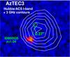 |
Fig. D.1 Hubble/ACS F814W (I-band) image towards AzTEC 3 shown with a logarithmic colour scaling, overlaid with contours showing the 3 GHz radio emission (starting at 3σ and increasing in steps of 1σ; see Paper II). The foreground galaxy, seen |


Based on the VLA and PdBI observations of multiple rotational lines of CO emission, Riechers et al. (2010) derived a gas mass of Mgas = 5.3 × 10¹⁰M⊙ for AzTEC 3 (αCO = 0.8M⊙ (K km s-1 pc2)-1 was assumed). Using the dust and stellar masses we derived, we obtain a gas-to-dust mass ratio of  , and a gas fraction of fgas = Mgas/ (Mgas + M⋆) ≃ 37%. The [C ii] luminosity reported by Riechers et al. (2014), L[C ii] = (6.69 ± 0.23) × 109L⊙, suggests a molecular gas mass of Mgas ~ 5.2−8.3 × 10¹⁰M⊙ (see Swinbank et al. 2012), i.e. only up to a factor of about 1.6 higher than the CO-based value from Riechers et al. (2010). The [C ii]-to-IR luminosity ratio for AzTEC 3,
 ![Mathematical equation: \hbox{$L_{[\ion{C}{II}]}/L_{\rm IR}=0.0002^{+0.0001}_{-0}$}](/articles/aa/full_html/2017/01/aa28128-16/aa28128-16-eq971.png) , is even lower than for AzTEC 1, and makes this SMG an object with an extreme [C ii] deficiency.
, is even lower than for AzTEC 1, and makes this SMG an object with an extreme [C ii] deficiency.
Assuming that AzTEC 3 has sustained its current SFR continuously, its stellar mass building-up timescale is  Myr, while the gas depletion timescale is
  Myr. For comparison, the MAGPHYS-based mass-weighted age of AzTEC 3 is about 22 Myr. A similarly short gas consumption timescale (20–30 Myr) is found for the z = 4.5 SMG J1000+0234 (Schinnerer et al. 2008), and the z = 4.05 SMG GN20, which is also a protocluster member (Daddi et al. 2009) that is similar to AzTEC 3 (Capak et al. 2011). Given the τdep/τbuild ratio of
  , we derive for AzTEC 3, its present stellar mass could have been fully built up during the current starburst episode, as concluded for AzTEC 1 above. The value of for AzTEC 3 is
  Gyr-1, and
  L⊙. The latter is consistent with the aforementioned Eddington limit of SFEEdd = 500L⊙.
Based on ALMA λrest = 158μm [C ii] observations, Riechers et al. (2014) derived a dynamical mass of Mdyn = 9.7 × 10¹⁰M⊙ for AzTEC 3. We can use the aforementioned gas mass and our new stellar mass to estimate the dynamical mass as Mdyn ≃ Mgas + M⋆ ≃ 1.4 × 10¹¹M⊙. This is only about 1.4 times higher than the [C ii]-based value from Riechers et al. (2014) and, given the uncertainty in the mass values, this discrepancy does not seem very significant. The final stellar mass of AzTEC 3 can be estimated to be M⋆, final = M⋆ + Mgas ≃ Mdyn ~ 1.4 × 10¹¹M⊙, and as found for AzTEC 1 above, AzTEC 3 could evolve into a massive elliptical galaxy in the present-day Universe.
The continuum size at λobs = 1 mm (λrest = 159μm) derived for AzTEC 3 by Riechers et al. (2014) through their ALMA observations is  (deconvolved FWHM). This corresponds to a physical rest-frame FIR FWHM size of
  kpc2. Using this size scale, we derive a SFR surface density of
  M⊙ yr-1 kpc-2, where the nominal value is 2.8 times higher than reported by Riechers et al. (2014; 530 M⊙ yr-1 kpc-2). Our ΣSFR value is consistent with the Eddington limit for a radiation-pressure supported starburst of M⊙ yr-1 kpc-2 (e.g. Andrews & Thompson 2011), and is hence in agreement with the aforementioned Eddington-limited SFE comparison. Similarly, using our IR luminosity value, we can derive a LIR surface density of
  L⊙ kpc-2. This value is similar to that expected for an optically thick starburst disk (~1013L⊙ kpc-2; Thompson et al. 2005). Besides the compact FIR size derived by Riechers et al. (2014), the high dust temperature we derived for AzTEC 3, K, suggests that star formation takes place on small spatial scales and, hence, the dust grains are subject to a strong radiation field (e.g. Yang et al. 2007; da Cunha et al. 2015). We searched for a correlation between the 3 GHz radio size and the MAGPHYS-based dust temperature among our SMGs, but only a weak relationship was found (the Pearson correlation coefficient was found to be r = −0.28, while 0 implies no correlation).
In their study of AzTEC 3, Dwek et al. (2011) concluded that the dust content of this SMG formed over a period of ~200 Myr with a constant SFR of ~ 500M⊙ yr-1 and a top-heavy IMF. We note that the dust mass they adopted in their analysis, Mdust = (2 ± 1) × 109M⊙, is only  times higher than the value we derived, but an upper limit of <5 × 10¹⁰M⊙ to the stellar mass they assumed is lower than the value of
  M⊙ we derived. Since AzTEC 3 is seen when the Universe was just 1.07 Gyr old, the high dust mass we derived for this source suggests an efficient dust production, but inefficient dust destruction, by supernovae (cf. the “dust-budget crisis” in high-z SMGs; Rowlands et al. 2014b).
All Tables
Comparison of the physical properties between the target AzTEC SMGs and the equally bright ALESS SMGs.
Classification of the target SMGs into different radio SED categories in the observed frequency interval 0.325–3 GHz.
Flux densities of our SMGs at the observed radio frequencies of 325 MHz, 1.4 GHz, and 3 GHz.
All Figures
|
Fig. 1 Best-fit panchromatic (UV-radio) rest-frame SEDs of 16 of our target SMGs. The source ID and redshift are shown on the top of each panel. The red points with vertical error bars represent the observed photometric data, and those with downwards pointing arrows indicate the 3σ upper flux density limits (taken into account in the fits). The blue line is the best-fit MAGPHYS model SED from the high-z library (da Cunha et al. 2015). All the SMGs, except AzTEC 21b, are detected in at least one radio frequency (see Fig. 2 for the pure radio SEDs). |
| In the text | |
|
Fig. 2 Radio SEDs (on a log-log scale) of 19 of our target SMGs that were detected in at least one of the three observed frequencies of 325 MHz, 1.4 GHz, and 3 GHz (the three data points in each panel with vertical error bars). The downwards pointing arrows show 3σ upper limits. The solid lines show the least squares fits to the data points, and the continuation of the fit is illustrated by the dashed line. The derived spectral index values are shown in each panel. In each panel, the lower x-axis shows the observed frequency, while the upper x-axis gives the corresponding rest-frame frequency (for AzTEC 6 and 27, only a lower z limit is available and, hence, the νrest shown is only a lower limit). |
| In the text | |
|
Fig. 3 Radio spectral index between 325 MHz and 3 GHz as a function of redshift. The arrows indicate lower and upper limits to |
| In the text | |
|
Fig. 4 Log-log plot of the SFR vs. stellar mass. The black squares show our AzTEC SMG data points, while the red filled circles show the ALESS SMG data from da Cunha et al. (2015), where the ALESS sample was limited to sources with similar flux densities as our sample (see Sect. 4.2 for details). The dashed lines show the position of the star-forming main sequence at the median redshift of the analysed AzTEC SMGs (z = 2.85; black line) and the flux-limited ALESS sample (z = 3.12; red line) as given by Speagle et al. (2014); the lower and upper black dashed lines indicate a factor of three below and above the main sequence at z = 2.85. |
| In the text | |
|
Fig. 5 Starburstiness or the distance from the main sequence (parameterised as SFR/SFRMS) as a function of redshift. The blue horizontal dashed line indicates the sample median of 4.6, while the green filled circles represent the mean values of the binned data (each bin contains four SMGs) with the error bars showing the standard errors of the mean values. |
| In the text | |
|
Fig. 6 3 GHz radio continuum sizes (radii defined as half the major axis FWHM) derived in Paper II (and scaled to the revised redshifts and cosmology adopted here) plotted against the stellar masses derived in the present work (black squares). The SMGs at z> 3 are highlighted by green star symbols. For comparison, the red squares show the rest-frame UV/optical radii from Toft et al. (2014; also scaled to the present redshifts and cosmology). The upper size limits are indicated by arrows pointing down. The three dashed lines show the mass-size relationship of z ~ 2 compact, quiescent galaxies from Krogager et al. (2014), where the lower and upper lines represent the dispersion in the parameters (see text for details). |
| In the text | |
|
Fig. 7 Infrared-radio correlation q ≡ qTIR parameter as a function of redshift. The arrows pointing up and down show the lower and upper limits, respectively. The green filled circles represent the survival analysis-based mean values of the binned data (each bin contains five SMGs) with the error bars showing the standard errors of the mean values. The blue dashed line indicates the median value of |
| In the text | |
|
Fig. 8 Specific SFR (sSFR) as a function of cosmic time (lower x-axis) and redshift (upper x-axis) for our SMGs and the flux-limited sample of ALESS SMGs. The plotted data points represent the mean values of our data and the ALESS SMG data binned in redshift and sSFR (each of our bin contains four sources, while the ALESS data have five values in each bin). The error bars represent the standard error of the mean. The horizontal dashed lines indicate the full sample median sSFRs of |
| In the text | |
|
Fig. 9 Dust-to-stellar mass ratio as a function of redshift for our SMGs and the flux-limited ALESS SMGs. The green filled circles represent the mean values of the binned AzTEC data (each bin contains four SMGs), while the cyan filled circles represent the mean values of the binned ALESS data (each bin contains five SMGs). The error bars of the binned data points represent the standard errors of the mean values. The horizontal dashed lines indicate the corresponding median values of |
| In the text | |
|
Fig. 10 Top: radio spectral index between 325 MHz and 3 GHz as a function of starburstiness or the distance from the main sequence (parameterised as SFR/SFRMS). For reference, the horizontal dashed line indicates the median spectral index value of |
| In the text | |
|
Fig. 11 Stellar mass distribution of our z> 3 SMGs (green histogram), and z ~ 2 cQGs (2014; red histogram). The blue histogram shows the distribution of the final stellar masses of the z> 3 SMGs by assuming that 10% of their putative gas mass content is converted into stars by the end of the ongoing starburst event, while the magenta dashed histogram represents the final stellar mass distribution where Mgas is based on the mass-metallicity relationship (see text for details). The CO-based gas mass estimate was adopted for AzTEC 1 and AzTEC 3 (Appendix D). |
| In the text | |
|
Fig. B.1 Best-fit panchromatic (UV-radio) rest-frame SEDs of five of our target SMGs. The source ID and redshift are shown on top of each panel. The red points with vertical error bars represent the observed photometric data, while those with downwards pointing arrows indicate the 3σ upper flux density limits. The blue line is the best-fit MAGPHYS model SED from the high-z library. |
| In the text | |
|
Fig. D.1 Hubble/ACS F814W (I-band) image towards AzTEC 3 shown with a logarithmic colour scaling, overlaid with contours showing the 3 GHz radio emission (starting at 3σ and increasing in steps of 1σ; see Paper II). The foreground galaxy, seen |
| In the text | |
Current usage metrics show cumulative count of Article Views (full-text article views including HTML views, PDF and ePub downloads, according to the available data) and Abstracts Views on Vision4Press platform.
Data correspond to usage on the plateform after 2015. The current usage metrics is available 48-96 hours after online publication and is updated daily on week days.
Initial download of the metrics may take a while.