| Issue |
A&A
Volume 592, August 2016
|
|
|---|---|---|
| Article Number | A132 | |
| Number of page(s) | 22 | |
| Section | Extragalactic astronomy | |
| DOI | https://doi.org/10.1051/0004-6361/201526563 | |
| Published online | 15 August 2016 | |
Ultramassive dense early-type galaxies: Velocity dispersions and number density evolution since z = 1.6
1 INAF–Istituto di Astrofisica Spaziale e Fisica Cosmica Milano, via Bassini 15, 20133 Milano, Italy
e-mail: This email address is being protected from spambots. You need JavaScript enabled to view it.
2 INAF–Osservatorio Astronomico di Brera, via Brera 28, 20121 Milano, Italy
3 Dipartimento di Scienza e Alta Tecnologia, Università degli Studi dell’Insubria, via Valleggio 11, 22100 Como, Italy
Received: 20 May 2015
Accepted: 3 May 2016
Abstract
Aims. We investigate the stellar mass assembly history of ultramassive (M⋆ ≳ 1011M⊙) dense (Σ = M⋆/2πRe2> 2500M⊙ pc-2) early-type galaxies (ETGs, elliptical and spheroidal galaxies) selected on basis of visual classification over the last 9 Gyr.
Methods. We traced the evolution of the comoving number density ρ of ultramassive dense ETGs and compared their structural (effective radius Re and stellar mass M⋆) and dynamical (velocity dispersion σe) parameters over the redshift range 0 < z < 1.6. We derived the number density ρ at 1.6 <z< 1 from the MUNICS and GOODS-South surveys, while we took advantage of the COSMOS spectroscopic survey to probe the intermediate redshift range [0.2−1.0]. We derived the number density of ultramassive dense local ETGs from the SDSS sample taking all of the selection bias affecting the spectroscopic sample into account. To compare the dynamical and structural parameters, we collected a sample of 11 ultramassive dense ETGs at 1.2 < z < 1.6 for which velocity dispersion measurements are available. For four of these ETGs (plus one at z = 1.91), we present previously unpublished estimates of velocity dispersion, based on optical VLT-FORS2 spectra. We probe the intermediate redshift range (0.2 ≲ z ≲ 0.9) and the local Universe with different ETGs samples.
Results. We find that the comoving number density of ultramassive dense ETGs evolves with z as ρ(z) ∝ (1 + z)0.3 ± 0.8 implying a decrease of ~25% of the population of ultramassive dense ETGs since z = 1.6. By comparing the structural and dynamical properties of high-z ultramassive dense ETGs over the range 0 ≲ z < 1.6 in the [Re, M⋆, σe] plane, we find that all of the ETGs of the high-z sample have counterparts with similar properties in the local Universe. This implies either that the majority (~70%) of ultramassive dense ETGs already completed the assembly and shaping at ⟨ z ⟩ = 1.4, or that, if a significant portion of dense ETGs evolves in size, new ultramassive dense ETGs must form at z < 1.5 to maintain their number density at almost constant. The difficulty in identify good progenitors for these new dense ETGs at z ≲ 1.5 and the stellar populations properties of local ultramassive dense ETGs point towards the first hypothesis. In this case, the ultramassive dense galaxies missing in the local Universe could have joined, in the last 9 Gyr, the so colled non-dense ETGs population through minor mergers, thus contributing to mean size growth. In any case, the comparison between their number density and the number density of the whole population of ultramassive ETGs relegates their contribution to the mean size evolution to a secondary process.
Key words: galaxies: elliptical and lenticular, cD / galaxies: evolution / galaxies: formation / galaxies: high-redshift
© ESO, 2016
1. Introduction
Most of the studies focusing on the structural parameters of massive, passive galaxies, both at high and at low redshift, indicate that this population of galaxies has increased the mean effective radius over the cosmic time (e.g. Daddi et al. 2005; Trujillo et al. 2006, 2007; Longhetti et al. 2007; Zirm et al. 2007; Toft et al. 2007; van Dokkum et al. 2008; Franx et al. 2008; Cimatti et al. 2008; Buitrago et al. 2008; van der Wel et al. 2008, 2014; Bernardi 2009; Damjanov et al. 2009; Bezanson et al. 2009; Mancini et al. 2009, 2010; Cassata et al. 2011; Damjanov et al. 2011; Bruce et al. 2012; Szomoru et al. 2012; Newman et al. 2012; Cassata et al. 2013; Belli et al. 2014). For example, van der Wel et al. (2014) find that the mean effective radius ⟨ Re ⟩ of passive galaxies selected with a colour−colour criterion increases as ⟨ Re ⟩ ∝ (1 + z)-1.48 over the redshift range 0 <z< 3. Similar results, among the others, have also been reached by Cassata et al. (2013) on samples of passive (specific star formation rate sSFR< 10-11 yr-1) galaxies, and by Cimatti et al. (2012) for galaxies with red colours and elliptical morphology. Nonetheless, other analyses contrast these results, showing a mild or an even negligible evolution of the mean size with cosmic time (Saracco et al. 2011, 2014; Stott et al. 2011; Jorgensen & Chiboucas 2013; Jorgensen et al. 2014; Poggianti et al. 2013a). Most of these works investigate a sample of galaxies selected on the basis of their elliptical morphology.
In fact, the reason for these different results is not easily detectable. A major point to be considered is that a selection based on the passivity (or on the Sersic index n> 2.5; see e.g. Buitrago et al. 2013) includes in the sample a significant portion (> 30%) of disk galaxies (e.g. van der Wel et al. 2011; Ilbert et al. 2010; Cassata et al. 2011; Tamburri et al. 2014) and, concurrently, does not include all of the galaxies that are visually classified as ellipticals. At the same time, a selection based on a cut in sSFR that is constant with time (usually sSFR< 10-11 yr-1) selects predominantly red spheroids at z ~ 2, but includes a large contamination of disk/spiral galaxies in the local Universe (Szomoru et al. 2011). Actually, Keating et al. (2015) show that the properties of high-z elliptical galaxies are highly sensitive to the definitions used in selecting the samples (see also Moresco et al. 2013).
In addition to this debated issue on the amount of evolution in size, its possible origin is also investigated. Is the increase of the mean size due to the growth in size of individual galaxies across the time, resulting from inside-out stellar matter accretion due to minor dry merging, or rather to the addition of new and larger galaxies over cosmic time (e.g. Valentinuzzi et al. 2010; Carollo et al. 2013)? A promising approach to shed light on the origin of the size evolution is to investigate how the number density of dense galaxies evolves over the cosmic time (Saracco et al. 2010; Bezanson et al. 2012; Cassata et al. 2013; Poggianti et al. 2013b; Carollo et al. 2013; Damjanov et al. 2014, 2015). The analyses by various authors differ slightly in the selection of the sample, for example via passivity, visual classification, colour, and Sersic index; in the definition of so-called dense galaxies, selected for example on the basis of their mean stellar mass density Σ = M⋆/2π or sigma deviation from the local size-mass relation (SMR); and in the treatment of the progenitor bias. Saracco et al. (2010) find that the number density of dense (1σ below the local SMR) massive (M⋆> 3 × 10¹⁰M⊙) ellipticals (visually selected) at 0.9 <z< 1.9 is comparable with that of equally dense massive ellipticals in local clusters. Similarly, Poggianti et al. (2013b), studying the number density of massive (M⋆ ≳ 1010M⊙), compact (Log (M⋆/
 ) ≥ 10.3 M⊙ kpc-1.5), local old galaxies, find that it is just a factor 2 lower than that of compact passive galaxies observed at z = 2. In contrast, van der Wel et al. (2014) find that the number density of dense (Re/(M⋆/1011M⊙) < 1.5 kpc), massive (M⋆> 5 × 10¹⁰M⊙), passive galaxies decreases by a factor ~10 from z ~ 2 at z ~ 0.2.
Actually, the individual size growth is expected to be more efficient for the most massive (M⋆> 1011) galaxies. In fact, these systems are expected to host the centre of the most massive halo and to evolve mainly through minor mergers (Hopkins et al. 2009). However, given the fact that at each redshift the most massive galaxies are extremely rare (see, e.g., Muzzin et al. 2013), very few works have investigated the number density evolution of their dense subpopulation over cosmic time. Carollo et al. (2013) find that the number density of passive (sSFR< 10-11 yr-1) and elliptical galaxies with M⋆> 1011M⊙ and Re< 2 kpc decreases ~30% in the 5 Gyr between 0.2 <z< 1. An even mild evolution is claimed by Damjanov et al. (2015), who find an almost constant number density in the range 0.2 <z< 0.8 for the passive (colour selected) and dense (Log (M⋆/) ≥ 10.3 M⊙ kpc-1.5) galaxies with M⋆> 8 × 10¹⁰M⊙.
A study still missing concerns the evolution of the number density of the population of “pure” elliptical (elliptical and spheroidal galaxies selected on the basis of visual classification), massive (M⋆> 1011M⊙), dense galaxies, in particular, at z> 0.8−1, which is the range in which most of the evolution of spheroidal galaxies occurs. From here on, with the term early-type galaxy (ETG) we identify an elliptical galaxy selected on the basis of visual classification, and with no other criterion (e.g. color, Sersic index, sSFR).
Main characteristics of the surveys used to derived the number density evolution from z = 1.6 to z ~ 0.
In this paper, we aim to probe the mass accretion history of these most massive and dense (M⋆> 1011M⊙, Σ > 2500 M⊙ pc-2) ETGs over the previous ~9 Gyr, by tracing the evolution of their comoving number density and comparing their structural and dynamical parameters from redshift 1.6 to ~0. One of the aspects of this work that differs from the previous analyses is the selection of the samples based on visual classification, or on a methodology that can mimic the visual classification, over the whole redshift range. In fact, the star formation histories of galaxies are often more complex than we are able to model them, as they are characterized by bursty against smooth and gentle declining star formation histories. As a consequence of this, in a phase of low star formation activity, an active galaxy can just “temporarily” show red colours and/or low sSFR. Moreover, galaxies tend to become passive with time. Hence, the population of passive galaxies collects a different mix of morphological types at different redshift. This leads to a non-homogeneous comparison of their properties at different time (see, e.g., Huertas-Company et al. 2013). In this context, the spheroidal shape of a galaxy is a more stable property over time and allows us to select the same population over cosmic time. In addition, we selected dense galaxies on the basis of their Σ rather then using a constant cut in Re or on the basis of their deviation with respect to the local SMR. The main reason for this choice is that the mean stellar mass density, up to z ~ 1.5, is better correlated to, for example the age, the sSFR of the galaxy (Franx et al. 2008; Wake et al. 2012) and hence constitutes a more meaningful parameter.
We organized the analysis into two parts.
First we focus (see Sect. 2) on the evolution of the number density of ultramassive dense ETGs over the redshift range 0 < z < 1.6 to investigate whether the ultramassive dense high-z ETGs are numerically consistent with those observed at z ~ 0 or, on the contrary, whether they numerically decrease along the time, which would suggest individual growth of galaxies. For this purpose, we have referred to SDSS DR4 survey to constrain the number density of ultramassive dense ETGs at z ~ 0.1, paying particular attention to the bias affecting the catalogue (see Sect. 2.3) and to COSMOS field to cover the range 0.2 ≲ z ≲ 1 (see Sect. 2.2). For the highest redshift bin (1.2 ≲ z < 1.6), we have considered two different surveys of similar area (~150 arcmin2), the GOODS-South (Giavalisco et al. 2004) and the MUNICS (Drory et al. 2001), to average over the cosmic variance (see Sect. 2.1).
In the second part of the paper, we focus on comparing the structural (i.e. Re, M⋆) and dynamical (i.e. velocity dispersion σ) parameters of ETGs over the last 9 Gyr (see Sect. 3). This analysis aims to asses whether high-z ultramassive dense ETGs have counterparts at lower z that are characterized by the same structural and dynamical properties or, rather, whether some of these are not present at later epochs. To perform this comparison, we selected data from the literature (see Sect. 3.1). Clearly, the request of available velocity dispersion drastically reduces the statistics of the sample at 1.2 < z < 1.6 to 11 ETGs. For four of these ETGs (plus one at z = 1.9), we present new measurements of velocity dispersions (see Sect. 3.1). In Sect. 4 we summarize the work and present our results and conclusions.
Throughout the paper we adopt standard cosmology with H0 = 70 km s-1 Mpc-1, Ωm = 0.3 and Ωλ = 0.7, the stellar masses we report are derived using the Chabrier initial mass function (IMF; Chabrier 2003) and the magnitudes are in the AB system when not otherwise specified.
2. The number density of ultramassive dense ETGs
In this section we constrain the stellar mass accretion history of ultramassive ETGs by investigating the evolution of their number density ρ over the last ~9 Gyr. We cover the redshift range from 1.6 to 0 with different surveys (e.g. with different magnitude cut and completeness) and in Table 1 we summarize their main characteristics, and the references for the main quantities involved in this part of analysis (i.e. stellar mass and Re). As a reminder, we highlight that this analysis aims to probe the evolution of ETGs, i.e. elliptical and spheroidal galaxies selected on the basis of the visual classification. When this classification is not feasible, we explicitly discussed this in the text.
2.1. The number density of ultramassive dense ETGs at 1 ≲z < 1.6
For the comoving number density of ultramassive dense ETGs at z> 1, we referred to two samples of ETGs: one selected in the MUNICS-S2F1 field, and published in Saracco et al. (2005) and Longhetti et al. (2007), and the other selected in the GOODS South-field and described in Tamburri et al. (2014).
MUNICS sample – The MUNICS sample consists of seven ultramassive dense ETGs spectroscopically confirmed at z ~ 1.5. These galaxies were observed as part of the spectroscopic follow-up of the complete sample of 19 extremely red objects (EROs; K ≲ 20.4, R−K ≲ 3.6) in the S2F1 field (Saracco et al. 2005). We checked whether the cuts both in magnitude and colour of the MUNICS sample affect our selection of ultramassive dense ETGs. Using the sample of ETGs in the GOODS-South field presented in Tamburri et al. (2014; see below), we verified that a sample of ETGs that is brighter than K = 20.4 is 100% complete up to z ~ 1.6. The colour cut tends to deprive the massive sample of the less dense systems (in which we are not interested), since the redder the colour of a galaxy, the higher its Σ (Franx et al. 2008; Saracco et al. 2011). All of the galaxies of the MUNICS sample, indeed, have Σ > 2500 M⊙ pc-2. The effective radii of the galaxies were derived in the F160W filter with GALFIT (Longhetti et al. 2007) and the stellar masses were estimated by fitting their spectral energy distribution (SED) with the Bruzual and Charlot models using the Chabrier IMF, while visual classification was performed on HST/NIC2 – F160W images (for more details see Sect. 3). We revised the number density estimated by Saracco et al. (2005) considering only the six ETGs at 1.2 <z< 1.6 in the field S2F1 (~160 arcmin2), thus, excluding the ETG S2F1-443 at z = 1.91 (see Sect. 3). We found a comoving number density of ultramassive dense ETGs of 3.8(±1.7) × 10-5 gal/Mpc-3 at 1.2 <z< 1.6, which becomes 5.6(±1.9) × 10-5 gal/Mpc-3 considering the spectroscopic incompleteness (a factor ~1.4). The errors on number densities, throughout the paper, are based on Poisson statistics.
GOODS – South sample – Given the small area of the S2F1-MUNICS field, for comparison, and to average the cosmic variance, we also derived the number density of ultramassive dense ETGs in the GOODS-South field covering an area (143 arcmin2) comparable to the S2F1 field. To this end, we used the sample of galaxies that are visually classified as ETGs on ACS/F850LP images and studied by Tamburri et al. (2014). The sample contains all of the ETGs in the GOODS-South field that are brighter than Ks = 22 and for masses M⋆> 1011M⊙ is 100% complete up to z ~ 2 (Tamburri et al. 2014). Their stellar masses were derived assuming Bruzual and Charlot models and both the Salpeter IMF and Chabrier IMF. We refer to the latter in our analysis. We found a number density of ultramassive dense ETGs of 1.8( ± 1.3) × 10-5 gal/Mpc3 in the redshift range 1.3 ≲ z< 1.6 and of 2.9( ± 1.6) × 10-5 gal/Mpc3 in the redshift range 0.95 <z< 1.25. The structural parameters in the Tamburri et al. sample were derived on the ACS-F850LP images with GALFIT. Hence the selection of ETGs could be biased against dense ETGs because of their larger apparent size (~30%, Gargiulo et al. 2012) at this wavelength. The number density of dense ETGs does not change, however, even when we correct the effective radius of massive ETGs in the GOODS sample for this difference. In Table 2 and in Fig. 2 we report the measures.
2.2. The number density of ultramassive dense ETGs at intermediate redshift
We took advantage of the COSMOS survey to derive the comoving number density of ultramassive dense ETGs at intermediate redshift. We have considered the catalogue of Davies et al. (2015), including all of the available spectroscopic redshifts in the COSMOS area, the catalogue of structural parameters based on the HST/ACS images in the F814W filter of Scarlata et al. (2007), and the catalogue including the stellar masses of Ilbert et al. (2013) based on the multiwavelength UltraVISTA photometry. The cross match of these three catalogues produced a sample of 110 171 galaxies in the magnitude range 19 <F814W< 24.8 over the 1.6 deg2 of the HST/ACS COSMOS field. We then selected all of the galaxies (25262) that are brighter than F814W< 22.5 mag for which structural parameters and morphological classification are robust (Sargent et al. 2007; Scarlata et al. 2007). We finally extracted our parent sample of 1412 galaxies with stellar mass M∗> 1011M⊙ and early-type morphology from this sample. We refer to the Zurich Estimator of Structural Types (ZEST) estimates by Scarlata et al. (2007) for the morphological classification. An automated tool for galaxy classification, ZEST uses the Principal Component Analysis to store the full information provided by the entire set of five basic non-parametric diagnostics of galaxy structure (symmetry, concentration, Gini coefficient, 2nd-order moment of the brightest 20% of galaxy pixels, and the ellipticity) plus the Sersic index. The software subdivided the galaxies into three main classes: early types (type = 1), disk galaxies (type = 2), and irregular galaxies (type = 3). The robustness of the software was tested both on ~56 000 COSMOS galaxies and on local galaxies that are visually classified, with excellent results. For our analysis, thus, we selected as COSMOS ETGs, all of the galaxies with ZEST-type = 1. Among these, 551 have a secure spectroscopic redshift (parameter Z_USE ≤ 2 in the Davies et al. 2014 catalogue), and 145, at 0.2 <z< 1.0, have Σ ≥ 2500 M⊙ pc-2. As a further check on morphology, we visually classified the 145 ultramassive dense COSMOS galaxies with ZEST-type = 1 on the HST/F814W-ACS images (Koekemoer et al. 2007). Actually, we found that all but one are ETGs.
The selection at F814W< 22.5 mag implies that for M∗> 1011M⊙ the sample is 100% complete up to z ~ 0.8 (80% complete to z ~ 1). The stellar masses of Ilbert et al. (2013) are based on the Bruzual and Charlot (2003) models and the Chabrier IMF, which is consistent with our assumptions. The structural parameters of Sargent et al. (2007) are based on a Sersic profile fitting as in our analysis even if performed with GIM2D instead of GALFIT. However, Damjanov et al. (2015) show that the two methods, GIM2D and GALFIT, are in excellent agreement when based on a single Sersic component, as in our case. To derive the number densities of massive ETGs, we applied a correction for the spectroscopic incompleteness that we defined as the ratio between the magnitude distribution (in bin of 0.1 mag) of the parent sample of ETGs and the sample of ETGs with spectroscopic redshift. In Table 2 we report the comoving number density of ultramassive dense ETGs from z = 0.2 to z = 1.0, estimated in bins of redshift of 0.2 (see also Fig. 2). At z> 0.6, the rest-frame wavelength sampled by the F814W filter is significantly different from that sampled by the filter F160W at z = 1.5. As carried out for the GOODS-south data, however, we verified that the number densities derived from the COSMOS data at z> 0.6 do not change even when we assume a correction of 30% of the effective radii of galaxies.
Number density ρ of ultramassive dense (M⋆> 1011M⊙, Σ > 2500 M⊙ pc-2) ETGs from z = 1.6 to ~0.
2.3. The number density of ultramassive dense ETGs in local Universe
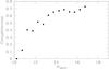 |
Fig. 1 Completeness of the spectroscopic SDSS galaxy catalogue with respect to the main galaxy sample as a function of galaxy Petrosian magnitude. |
As representative sample of local ETGs we chose the dataset analysed by Thomas et al. (2010)1. These authors collected a sample of 16502 ETGs extracted from the magnitude-limited sample (r< 16.8) of 48023 galaxies selected from the SDSS data release 4 (Adelman-McCarthy et al. 2006) in the redshift range 0.05 ≤ z ≤ 0.1. Contrary to the other available samples, as our sample of high-z ETGs, this is the only sample in which ETGs are selected through a visual inspection of SDSS multiband images. The sample is 100% complete at M⋆> 1011M⊙. We associated with each ETG its stellar mass taken from MPA-JHU catalogue2 and obtained through the fit of the multiband photometry (Chabrier IMF), as for higher redshift galaxies. We have adopted as reference the NYU-VAG catalogue (Blanton et al. 2005) for the effective radius. In Appendix A, we discuss the robustness and limits of these estimates.
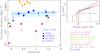 |
Fig. 2 Left: evolution of the comoving number density of ultramassive dense ETGs (M⋆ > 1011M⊙, Σ > 2500 M⊙ pc-2) from redshift 1.6 to redshift ~0 (blue symbols). The open blue square indicates the number density of ultramassive dense MUNICS ETGs at ⟨ z ⟩ = 1.4 corrected for the spectroscopic incompleteness of the MUNICS survey (see text). Solid blue line is the best-fit relation to our data in the range 0.066 < z < 1.6 (ρ ∝ (1 + z)0.3), while the blue dotted line indicates the mean value over the redshift range 0.066 < z < 1.6 (the dashed area indicates the 1σ deviation around this value). The orange squares indicate the number density for ultramassive compact galaxies by Damjanov et al. (2015), the magenta square by Trujillo et al. (2009), the light green square by Valentinuzzi et al. (2010), the purple squares by van der Wel et al. (2014), the salmon squares by Bezanson et al. (2009), the dark green square by Cassata et al. (2013), and the open red square by Taylor et al. (2010a). The points by Taylor et al. (open red square) and Cassata et al. (dark green square) are derived selecting from their sample only the galaxies with M⋆ > 1011M⊙ (see Table 3). The filled red square is the number density by Taylor et al. obtained using the circularized Sersic Re. Right: cuts in Re and M⋆ of our sample and other samples in the size to mass plane (colours are the same in the left panel). |
We bear in mind that the galaxy spectroscopic SDSS survey is biased against dense galaxies (e.g. Strauss et al. 2002; Poggianti et al. 2013a; Taylor et al. 2010b). Briefly, the main galaxy sample (MGS) of galaxy target for the spectroscopic follow-up is composed of all of the galaxies detected at >5σ in the r-band with Petrosian magnitude mpet,r< 17.77 and r-band Petrosian half-light surface brightness >24.5 mag arcsec-2. On these first cuts, three further selection criteria have been imposed to reject stars, avoid the cross talk, and exclude bright objects that can saturate the CCD. Taylor et al. (2010b) investigated how these cuts affect the distribution of local galaxies in the size mass plane and demonstrated that at z< 0.05, galaxies with masses and sizes similar to those of z ~ 2 galaxies are not targeted for the spectroscopic follow-up. Nonetheless, this incompleteness decreases at increasing redshift: at z ≳ 0.06, on average, the completeness of the spectroscopic survey for compact massive galaxies is ~80%. For this reason, we selected all of the ultramassive dense ETGs at 0.063 <z< 0.1, which amounts 156 galaxies, from the Thomas et al. catalogue. Based on the evidence of Fig. A.2 we removed from this sample 22 galaxies classified as ultramassive outliers in Appendix A, i.e. galaxies that should not be included in the local ultramassive sample since, most probably, their stellar masses derived through the SED fitting are overestimated. We visually checked this final subsample of 124 galaxies (156−22) and found that no galaxy has a close companion, is in the halo of a bright star, or is involved in a merger; these factors that can alter the estimate of the effective radius. However, we noted that ~15% of the sample (20 galaxies) does not have a clear elliptical or S0 morphology, even though they are included in the Thomas et al. ETG sample. We checked the structural parameters of these galaxies and they have a mean Sersic index n ≃ 3.5 (for all of the galaxies n> 2.5) that is consistent with the light profile of a spheroidal galaxy, but an axis ratio of b/a< 0.4. Since the Blanton catalogue does not provide an axis ratio, we used that obtained from the SDSS pipeline, fitting the real galaxies with a de Vaucouleur profile. Actually, the b/a should be not dependent on the surface brightness law used to fit the profile. We left these elongated objects in the final sample, since the Thomas et al. sample is widely adopted and studied, but in Sect. 2.4 we show that this choice does not impact our results.
Aside from this source of incompleteness due to the target selection, we have to consider that not all of the spectroscopic targets were actually observed (for example because two fibres cannot be placed closer than 55′′ on a given plate). This source of incompleteness should be more important for the brightest galaxies and should be taken into account in the derivation of the comoving number density. To quantify this incompleteness we extracted the MGS from the DR4 database restricting the query to only the sciencePrimary objects in order to reject multiple observations (648 852 galaxies). From this sample, we rejected galaxies classified as quasars leaving with 636980 galaxies. Among these objects, 384 564 (~60%) have been spectroscopically observed and ~88% of them have secure redshifts (i.e. zwarning = 0). We defined the completeness in bins of magnitude as the ratio of galaxies with secure redshift over the number of galaxies in the MGS (see Fig. 1). Taking this in consideration, we found a number density for local ultramassive dense ETGs of 0.75(±0.07) × 10-5 gal/Mpc-3. We repeated the measure of ρ, assuming as stellar masses for local ETGs those derived by Kauffmann et al. (2003) with spectral indices (see Appendix A) and we found ρ = 0.7(±0.06) × 10-5 gal/Mpc-3 . We corrected the number density for the incompleteness of the spectroscopic sample with respect to the MGS but the original selection cuts of the MGS can exclude part of massive dense ETGs especially in the lowest redshift bin. The number density we quote is therefore a lower limit.
2.4. The number density evolution of ultramassive dense ETGs over the last 9 Gyr: results
Figure 2 shows the evolution of number density for the ultramassive dense ETGs in the last ~9 Gyr. Once the possible sources of non-homogeneity are taken into account the mean value of the number density of ultramassive dense ETGs, within the uncertainties, is ~3.0 ± 1.5 × 10⁻⁵ Mpc-3. We observe that at z ~ 0.8, in the COSMOS field, there is a significant overdensity (see e.g. Damjanov et al. 2015, and reference therein) and that, correspondingly, this is the point that most deviates in Fig. 2. We fitted the number densities estimated in the redshift range 0.06 ≲ z< 1.6 with a power law, treating the SDSS and MUNICS point as lower limits, and found ρ(z) ∝ (1 + z)0.3 ± 0.8, showing that the number density of ultramassive dense ETGs may decrease from z = 1.6 to z = 0, approximately by a factor 1.3. We repeated the fit excluding from local sample those galaxies with ambiguous morphology (see Sect. 2.3), but the slope does not change, since in the fit this point is considered a lower limit.
2.5. Comparison with previous works
The number density estimates of dense ETGs are clearly dependent on many factors, such as the stellar mass limit, the definition of compact galaxies, and the criteria adopted to select the sample (e.g. visual classification, colour, and passivity). This implies that any comparison of our results with those by other authors is not straightforward. In the following we try to compare our estimates of number density with those by other authors that adopted selection criteria as similar as possible to ours. Given the many factors concurring in the final estimate of ρ, in Fig. 2 we report, in the size mass plane, the stellar mass and effective radius limits of each sample to better visualize these comparisons. At the same time, Table 3 immediately shows the characteristics of all of the samples studied.
2.5.1. Local Universe
For what concerns the local Universe, there is a clear tension among the results already published, since the number densities derived from the SDSS database (Trujillo et al. 2009; Taylor et al. 2010a) turn out to be at least 1−2 order of magnitude lower than those derived from other databases (e.g. WINGS/PM2GC; Valentinuzzi et al. 2010; Poggianti et al. 2013b, see Fig. 2). Interestingly, Fig. 2 shows that our estimate of local number density, although derived from the SDSS database, is much more in agreement with the finding of Valentinuzzi et al. (2010) than with that by Trujillo et al. (2009) and Taylor et al. (2010a). In the following, we investigate the possible origins of the observed discrepancy.
In fact, Taylor et al. (2010a) search for counterparts of high-z compact massive galaxies in the DR7 SDSS spectroscopic database. To this aim, they select from the sample of local galaxies at 0.066 <z< 0.12, with M⋆> 1010.7M⊙, and log(Re,z/kpc) < 0.56 × (log(M⋆/M⊙)−9.84)−0.3, i.e. with radius in the SDSS-z band at least twice as small as the local SMR by Shen et al. (2003), those with 0.1(u−r) > 2.53 to select the descendant candidates of high-z dense galaxies. They reject from their sample all of the galaxies with possible problems with their size measurement (due to confusion with, e.g. other galaxies, with extended halos, and/or with spikes of bright stars) or mass estimate, for a total final sample of 63 galaxies. Among these galaxies, 11 have stellar mass >1011M⊙ and yield a number density of 1.3(±0.4)10-7 gal/Mpc3 over the entire volume of the SDSS-DR7 spectroscopic survey (see Fig. 2 open red square). This value, which is not corrected for the spectroscopic incompleteness of SDSS-DR7 survey, is ~two orders of magnitude lower than the value we found. Actually, this huge observed difference cannot only be ascribed to the completeness function. In fact, it is really difficult to pinpoint the origin of such a difference between our result and their result, since the two samples are selected differently.
In fact, the cut they apply in Re is very similar to our cut in Σ (see size mass plane in Fig. 2), however, unlike us, they select only red galaxies. To test the impact of the colour selection, we computed the 0.1(u−r) colour for the galaxies of our sample and found that all but one have 0.1(u−r) > 2.5, so the colour selection cannot be the source of the observed difference in the number density. We then investigated the impact on the number density of the different Re used. Actually, we use the circularized Re obtained fitting the surface brightness profile with a Sersic law (hereafter Re,Ser), instead of the semi-major axis SMe, used by Taylor et al., obtained from SDSS pipeline fitting the SDSS images with a de Vaucouleur profile (hereafter SMe,dV). For this reason, we repeated their analysis looking for differences in the ρ estimates varying the definition of Re. To do this, we selected the 226312 galaxies with secure redshift (i.e. zwarning = 0) and spectroscopic redshift 0.066 <zspec< 0.12 from the primary observations of the DR7 spectroscopic sample. Among these, we collected those with M⋆> 1011M⊙, log(SMe,dV/kpc) < 0.56 × (log(M⋆/M⊙) −9.84) −0.3, and 0.1(u−r) > 2.5. For the SMe,dV we retrive the catalogue from the SDSS database, consistently with Taylor et al., while for the stellar masses derived through the SED fitting, we refer to the MPA-JHU catalogue (see Sect. 2.3). We visually inspected this subsample, and we rejected all of the galaxies with problems related to the size measurement (e.g. merging galaxies, or close pairs or galaxies in the halo of a bright stars), leaving us with 49 galaxies. None of these galaxies is a quasar. To check the reliability of the stellar mass estimates, we applied the same procedure as in Appendix A. Among the 49 galaxies of our selection, 38 have a stellar mass estimate that is also derived from the spectral indices (stellar masses from spectral indices were only derived for galaxies in the DR4 database), and for ten of these (~26%), the two estimates are consistent. These ten galaxies are all included in the subsample of 11 massive galaxies of Taylor and collaborators. Assuming that the fraction of galaxies with consistent estimates of M⋆ is constant, we should expect ~12 galaxies (49 × 0.26) with M⋆> 1011M⊙, log(SMe,dV/kpc) < 0.56×(log(M⋆/M⊙) −9.84)−0.3, 0.1(u−r) > 2.5 in DR7 release, in agreement with Taylor and collaborators. When circularized SDSS de Vaucouleur radii (Re,dV) are used instead, we found 569 galaxies with M⋆> 1011M⊙, log(Re,dV/kpc) < 0.56 × (log(M⋆/M⊙) −9.84)−0.3, 0.1(u−r) > 2.5, among which 186 have good Re estimates and stellar mass, against the 12 found when semi-major axes are used. Finally, when we use the Blanton Re,Ser (circularized and obtained fitting a Sersic profile), we find 687 galaxies with M⋆> 1011M⊙, log(Re,Ser/kpc) <0.56 × (log(M⋆/M⊙) −9.84) −0.3, and 0.1(u−r) > 2.5, which after all of the checks and visual inspection, result in a final sample of ~224 galaxies, which is a factor >20 higher than that obtained using the semi-major axis. The higher number of galaxies we have found using Re,Ser with respect to the one obtained using circularized de Vaucouleur radius is consistent with the expectations. Compact galaxies are known to generally have Sersic index n< 4, thus, the value of Re obtained fitting a de Vaucouleur profile should be higher with respect to that obtained fitting a Sersic law. This implies that the number of compact objects, which is defined using a Sersic-Re should be greater than that obtained using a de Vaucouleur-Re, as we find. For more details on the comparison of the local samples selected using circularized Re and semi-major axis (SMe), or de Vaucouleurs and Sersic Re see Appendix B. Thus, these checks show that the much lower number density found by Taylor et al. with respect to our estimate is because that they use the semi-major axis. Once the circularized Sersic Re values are used, the number density (not corrected for spectroscopic incompleteness) increases up to 2.6(±0.2)10-6 gal/Mpc-3 and is qualitatively in agreement with our estimate.
Trujillo et al. (2009), from the analysis of the SDSS DR6 database, claim that only the 0.03% of galaxies at z< 0.2 with M⋆> 8 × 10¹⁰M⊙ have 0.05″ <Re<1.5 kpc. We found that among the 99 783 galaxies in the SDSS DR4 spectroscopic sample with z< 0.2, zwarning = 0 and M⋆> 8 × 10¹⁰M⊙, only 113 (i.e. ~0.11% of the massive sample) have 0.05″ <Re< 1.5 kpc. The visual inspection rejects 76 galaxies, for example in the halo of a bright star or a merger galaxy. This leaves a sample of 37 galaxies, i.e. the 0.037% (versus 0.03% by Trujillo) of the original sample of local galaxies with M⋆> 8 × 10¹⁰M⊙. In this case, thus, the difference we found between our estimate and that by Trujillo et al. is totally ascribed to the different selection criteria. The authors probe a region of the size-mass plane that is included in our region (see size mass plane in Fig. 2) and known to be highly incomplete in the SDSS spectroscopic survey. Both factors lead to a very low number density.
Valentinuzzi et al. (2010), studying the sample of 78 clusters included in the WINGS survey, have derived the number density of local (0.04 <z< 0.07) galaxies with 8 × 10¹⁰<M⋆< 4 × 10¹¹M⊙ and Σ > 3000 M⊙ pc-2. Assuming there are no dense massive galaxies outside the clusters, they found a hard lower limit to the number density of these systems of 0.46 × 10⁻⁵ gal/Mpc-3. Using the DR7, we found 181 galaxies in the same z/M⋆/Σg range, where Σg is the mean stellar mass density derived using the effective radius measured by Blanton on SDSS g-band images, i.e. the SDSS band that is closer to the v-band used by Valentinuzzi et al. (2010). Among the 181 selected galaxies, 120 have reliable structural parameters, and ~64% of them has a robust stellar mass estimate. Taking the effect of the incompleteness into account, we found that the number density is ρ = 5.21 × 10⁻⁵ gal/Mpc3, thus a factor 10 higher than the lower limit of Valentinuzzi et al. (2010). Our estimate is in the right direction with respect to that of Valentinuzzi, but we are not in the position to make a more quantitative comparison. We avoid comparing our results with other analyses (e.g. Poggianti et al. 2013b) which, although treating the evolution of the number density of compact galaxies, adopt a much lower cut in stellar mass with respect to our cut (e.g. ~1−5 × 10¹⁰M⊙).
2.5.2. Intermediate redshift range
Carollo et al. (2013) derive the number density of M⋆> 1011M⊙ quenched (sSFR< 1011 yr-1) and elliptical galaxies with Re< 2.5 kpc over the redshift range 0.2 <z< 1 and find that it decreases by a factor ~30%. Their analysis is focused on a sample of galaxies, on average, denser than the one studied here, and differently from us they do not consider all the elliptical galaxies, but the subsample of passive ones. Despite this, their trend is in fair agreement with our findings. In fact, we find a decrease of ρ of ~20% in the redshift range 0.2 <z< 1.0.
Damjanov et al. (2015) present the number density of quiescent (colour–colour selected) galaxies with Log(M⋆/ kpc-1.5 and M⋆> 8 × 10¹⁰ in the COSMOS field and find that it is roughly constant in the redshift range 0.2 <z< 0.8. Their sample includes our one, thus, as expected their number density values are higher than those we find, but once again, their trend of ρ with z is in fair agreement with us. Actually, from z = 0.8 to z = 0.2 we find that ρ decreases by ~10%.
Finally, Tortora et al. (2016) derived the number density of massive (M⋆> 8 × 10¹⁰M⊙), supercompact (Re< 1.5 kpc) elliptical galaxies they detected in the Kilo Degree Survey. Although their compactness criterion is more restrictive than our criterion, the authors found an almost constant trend in the redshift range 0.2 ≲ z ≲ 0.6, consistently with our results.
2.5.3. High redshift
Bezanson et al. (2009), integrating the Schechter mass function given in Marchesini et al. (2009), find that the number density of the galaxies with M⋆> 1011M⊙ is 7.2 Mpc-3 at z = 2.5. Assuming that approximately half of the galaxies with M⋆> 1011M⊙ are compact, they find that the number density of compact massive galaxies at z = 2.5 is 3.6
 Mpc-3. The authors assume the Kroupa (2001) IMF, which provides stellar masses a factor ~1.2 higher than that obtained assuming the Chabrier IMF, so their value is an upper limit with respect to our values. The estimate by Bezanson et al. (2009) at z = 2.5 is in agreement with the mean value we find at z< 1.6 and with our best fit.
Cassata et al. (2013) derive the number density of compact (i.e. 1σ below the local SMR) and ultracompact (more than 0.4 dex smaller than local counterparts of the same mass) passive (sSFR< 10-11 yr-1) galaxies with elliptical morphology and M⋆> 1010M⊙ in the ~120 arcmin2 of the GOODS-South field covered by the first four CANDELS observations (Grogin et al. 2011; Koekemoer et al. 2011) and by the Early Release Science Program 2 (Windhorst et al. 2011). Using their published sample of 107 galaxies, we selected the only two galaxies with M⋆> 1011M⊙ and Σ > 2500 M⊙ pc-2 at 1.2  , which account for a number density of 1.47(±1.04)10-5 gal/Mpc3. This value is slightly lower than the value we found in the GOODS – South field (see Table 1), nonetheless we bear in mind that the authors selected passive and elliptical galaxies while we apply a pure visual classification. In comparing the sample of passive galaxies with that of elliptical galaxies that were visually classified, in the GOODS – South field, Tamburri et al. (2014) have shown that about ~26% of ETGs have sSFR> = 10-11 yr-1, i.e. are not passive. Taking this into consideration, we corrected the number density by a factor 1.26, obtaining 1.85(±1.30) × 10-5 gal/Mpc3, which is in agreement with our estimate on the GOODS – South field. The agreement between our number density estimate and that from the Cassata sample, although on the same field, is not straightforward. Actually, we derived all of the quantities involved in our estimate (e.g. stellar mass and effective radius) independently. Despite the different approaches and procedures, the number densities are consistent, thereby reinforcing the robustness of the result.
In the 3D-HST survey, van der Wel et al. (2014) derive the number density of compact (Re/(M⋆/1011M⊙)0.75< 1.5 kpc) passive (on the basis of their UVJ colours) galaxies with M⋆> 5 × 10¹⁰M⊙ in the redshit range 0 <z< 3. In contrast with our findings, the authors find a decrease by a factor ≳10 from z = 1.6 to z = 0. We have to premise that a reliable comparison with their work is unfeasible given the much different criteria used to select the samples, so we cannot go deeper into the orgin of the drop, which could be due, for example, to the different stellar mass limit (M⋆> 5 × 10¹⁰M⊙ vs. M⋆> 1011M⊙) and/or to a peculiarity of the population of red galaxies; in principle, we have no reason to suppose that the formation and evolutionary picture of ultramassive dense ETGs is similar to that of less massive and red galaxies. We find it jarring, however, that the values they find are a factor >5 lower than ours, despite their more relaxed cut in stellar mass. In the following we simply try to understand the origin of this discepancy. The criterion they adopted to select compact galaxies is very similar to our criterion (see Fig. 2), along with the reference rest-frame wavelength for the Re (r-band for us and 5000 Å for them). Thus, the reasons for the huge discrepancy we observe cannot reside in these features. There are two main differences between our approaches. First, they used the semi-major axes SMe instead of the Re. Second, they did not directly measure the semi-major axis on images sampling the 5000 Å rest frame at the various redshift considered, but they derived it from the SMe,F125W (i.e. the semi-major axis measured on the F125W-band images) assuming a variation with λ(Δlog SMe/Δlog λ) = −0.25 (see their Eq. (2)). In order to investigate whether one of these aspects (or both) are responsible for the observed discrepancy, we used our sample of ETGs selected in the GOODS-South field by Tamburri et al. (2014) and derived the number densities of ultramassive dense ETGs following the recipe by van der Wel et al. (2014). In details, we associated the structural parameters derived by van der Wel in both the F125W and F160W filter with each galaxy of our sample. From these we estimated the Re,5000 Å der, and SMe,5000Å der, following their Eq. (2). In the redshift range 0.95 < z < 1.25 in the GOODS South field we found three galaxies with M⋆ ≥ 1011M⊙ and Σ ≥ 2500 M⊙ pc-2 (see Table 2), while there are no ETGs using Re,5000 Å der and SMe,5000Å der. At 1.3 < z < 1.6 we found two galaxies. We found the same number of objects using Re,5000 Å der, and just one using the semi-major axis SMe,5000Å der. Thus, applying the same procedure by van der Wel et al. to derive the number density of ultramassive dense ETGs we find values of ρ lower or comparable (and no higher) than those presented in their paper; hence this is much more consistent with the expectations, considering the fact that our cut in stellar mass is more restrictive (for a more exaustive analysis on the effect of the extrapolation of the SMe using the van der Wel et al. Eq. (2), see Appendix C). However, we should keep in mind that in this comparison both the cosmic variance, and also the different selection of the sample (elliptical versus passive) have a strong effect on the number density estimates. All of these checks highlight the huge impact of the criteria and quantities used in each analysis on the comparison of the results. A fair comparison is really hard to address and this stresses the impelling necessity of analysis on homogeneous samples over cosmic time to draw firm conclusions.
3. The evolution of structural and dynamical parameters of ultramassive dense ETGs
The mild evolution in the number density shows that in the local Universe, the ultramassive dense ETGs are at most ~25% less numerous than at ⟨ z ⟩ = 1.4. Thus, if a significant portion of ultramassive dense ETGs evolves in size, new ETGs have to appear at lower redshift to maintain their number density as almost constant. The observed mild number density evolution also opens to the possibility that most (~75%) of the ultramassive dense ETGs passively evolve from ⟨ z ⟩ = 1.4 to z = 0. In this case, local and high-z ultramassive dense ETGs should also share the same structural and dynamical properties. In the following we compare the structural (Re and M⋆) and dynamical properties (σe) of the ultramassive dense ETGs over the last 9 Gyr. We highlight that in this second part of analysis, we investigate the same class of objects studied in Sect. 2, that is ETGs visually classified with M⋆> 1011M⊙ and Σ > 2500 M⊙ pc-2. The request of available velocity dispersion, however, does not allow us to use the same samples presented in Sect. 2. In Sect. 3.1 we present the samples used for this part of the analysis.
Sample of high-z ETGs collected from literature.
Our sample of high-z ETGs.
3.1. The comparison samples
In order to compare the structural and dynamical properties of ultramassive dense ETGs over the last 9 Gyr, we still refer, as local reference, to the sample of 124 ETGs presented in Sect. 2.3; this section also provides the stellar mass and effective radius used. For the velocity dispersions we referred to DR7 σ since in DR7 there have been improvements to the algorithms that photometrically calibrate the spectra and all spectra were re-reduced (see Thomas et al. 2013 for more tests on the reliability of DR7 σ estimates).
For the intermediate and high-z sample, we cannot refer to the same samples used to estimate the number density in Sect. 2, since not all of the ETGs have available velocity dispersions. We refer to the sample of field and cluster ETGs published by Saglia et al. (2010) to probe the intermediate redshift range (0.2 ≲ z ≲ 0.9). The authors selected the galaxies of their sample on the basis of their spectra (requesting the total absence or the presence of only weak [OII] lines), and they also provided the morphological classification (T type) for those with HST images. We selected from their sample, the galaxies with elliptical morphology (T type  ) and with M⋆ > 1011M⊙ and Σ > 2500 M⊙ pc-2. The stellar mass provided by the authors are derived adopting a diet Salpeter IMF. We converted these estimates to Chabrier IMF, scaling the masses by 0.085 dex. For the majority of the galaxies, the structural parameters were derived from the F814W-band images, while I-band VLT images were used for a small fraction of galaxies. We integrated the Saglia et al. sample, with that by Zahid et al. (2015), in which passive galaxies are selected on COSMOS field using a NUVrJ colour−colour cut. Using the coordinates of the galaxies available at the website4 of the author, we visually checked their morphology on HST/ACS images, finding that all but one passive galaxy are ellipticals.
For the high-z sample, we collected all of the high-z ETGs at 1.2 < z < 1.6 with Σ > 2500 M⊙ pc-2, M⋆ > 1011M⊙, available kinematics (i.e. velocity dispersion) and effective radius derived in the F160W band (11 objects). We performed the morphological classification on the basis of a visual inspection of the galaxies carried out on the HST images in the F160W filter. Among the 11 galaxies of the total high-z sample, seven galaxies were taken from the literature (see below) and, for the remaining four (plus one at z = 1.9, hereafter “our sample of high-z ETGs”), we present the unpublished VLT-FORS2 spectra together with their velocity dispersion measurements (Sect. 3.2). The seven galaxies from literature include as follow:
-
Four ETGs taken from Bezanson et al. (2013). From the eight galaxies of their sample we removed the galaxy U53937 bacause it is less massive than 1011M⊙, U55531 since its image shows that is not an elliptical, and C13412 and C22260, which have Σ < 2500 M⊙ pc-2.
-
Two ETGs taken from Belli et al. (2014). From the 56 quiescent galaxies of their sample, we excluded 23 passive galaxies that have z < 1.2; of the remaining 33, 24 were rejected because they had M⋆ < 1011M⊙, three were not ETGs (4906, 34609 and 34265), and four (1244914, 2823, 34879, 7310) had Σ < 2500 M⊙ pc-2.
-
One ETG taken from Longhetti et al. (2014). This galaxy belongs to MUNICS sample of six ETGs described in Sect. 2.1 and is used to estimate the number density.
The sample is summarized in Table 4. We do not include the three ETGs out of 17 galaxies presented in Newman et al. (2010) (ID GN3, GN4b, GN5b) with available σ, redshift z> 1.26 and M⋆> 1011M⊙, since their effective radii were derived fitting a de Vaucouleur and not a Sersic profile.
3.2. Our sample of high-z ETGs: spectroscopic observations and velocity dispersion measurements
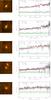 |
Fig. 3 Left column: HST-NIC2/F160W images of the five ETGs of our high-z sample for which we present the VLT-FORS2 spectra (each image is 6×6 arcsec). Right column: spectra, unsmoothed and not-rebinned, of our five ETGs (black lines, 8 h of effective integration time). Many optical absorption features (blue lines) are clearly distinguishable from the continuum. The best-fit pPXF model is plotted in red. On average, pPXF selects and combines 2−4 star templates to reproduce the observed spectrum. Residuals after best-fit model subtraction are shown with green points. In the residual tracks, blue lines are the regions automatically excluded by the software pPXF as strongly affected by sky emission lines. |
We selected the remaining four (plus one at z = 1.91) ETGs of the total high-z sample (Fig. 3, HST-NIC2/F160W images from Longhetti et al. 2007) among the seven ultramassive dense ETGs spectroscopically identified at z ~ 1.5 in the field S2F1 of the MUNICS survey (Drory et al. 2001); thus, they belong to the MUNICS sample we used to constrain the number density of ultramassive dense ETGs at z ~ 1.4 (see Sect. 2.1). Their surface brightness profiles are derived by Longhetti et al. (2007) fitting the HST-NIC2/F160W images with a 2D-psf convoluted Sersic law with the software GALFIT (Peng et al. 2002). In Table 5 we report the effective radii of the best-fitted Sersic profile for the five ETGs. The circularized Re [kpc] are slightly different from those published in Longhetti et al. (2007) because of the more accurate estimates of the redshift that we derived from the higher resolution VLT-FORS2 spectra. We re-estimated stellar masses to take the updated value of redshift and the now available near-IR photometry in the WISE RSR-W1 filter (λeff ≃ 3.4μm) into account. We considered a grid of composite stellar population templates derived from Bruzual & Charlot (2003) with solar metallicity Z⊙, exponentially declining star formation history (∝exp(−t/τ)) with star formation timescale τ in the range 0.1−0.6 Gyr, and the Chabrier IMF (Chabrier 2003). The effect of dust extinction has been modelled following the Calzetti law (Calzetti et al. 2000) with AV in the range [0.0−2.0]. The stellar masses M⋆ associated with the best-fit model are reported in Table 5. For the estimates of the number density derived in Sect. 2 we referred to these updated values of Re and M⋆.
Spectroscopic observations of our five ETGs were performed with the ESO VLT-FORS2 spectrograph in MXU mode during four runs in 2010 and 2011. The OG590 filter and the GRIS-600z grism were adopted to cover the wavelength range 0.6 μm <λ< 1.0 μm with a sampling of 1.6 Å per pixel. With a 1′′ slit the resulting spectral resolution is R ≃ 1400, corresponding to a FWHM ≃ 6.5 Å at 9000 Å. The total effective integration time on target galaxies is ~8 h, which results in signal-to-noise (S/N) per pixel ~[8−10] depending on the galaxy. Standard reduction was performed with IRAF tasks. In each frame the sky was removed by subtracting from each frame the following one in the dithering observing sequence. The sky-subtracted frames were aligned and co-added. The final stacked spectra were corrected for the response sensitivity function derived from the spectrum of the standard stars (FFEIGE110, GD71) observed in each of the four runs. Finally, we applied a further correction to the relative flux calibration related to the x-position of the slit on mask (Lonoce et al. 2014). In Fig. 3 the black lines show the 8-h, one dimensional spectra of our galaxies, which are not rebinned and unsmoothed.
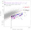 |
Fig. 4 Distribution of the ultramassive dense ETGs from z ~ 1.6 to z ~ 0 in the Re–M⋆ plane. Ultramassive dense ETGs at 1.2 <z< 1.6 are represented with magenta filled circles. The ETGs from MUNICS sample with available velocity dispersion (five presented here and one in Longhetti et al. 2014) are indicated with black countours. The ETG of MUNICS sample at redshift 1.91 (hence not included in the analysis of Sect. 3.3) is indicated with a blue point. Ultramassive dense ETGs at 0.3 <z< 0.9 and in the local Universe are indicated with blue open triangles and dark grey points, respectively. Solid black lines define the cuts in M⋆ and Σ of our samples. The small open circles show local ETGs from Thomas et al. (2010) in the redshift range 0.063 <z< 0.1. The red line indicates a line of constant σ derived as |

For the velocity dispersion (σ) measurements, we adopted the Penalized Pixel-Fitting software (Cappellari & Emsellem 2004, pPXF), which derive the σ by fitting the continuum and absorption features of the spectrum. We derived the velocity dispersions from the unbinned spectra, weighting each pixel for a quantity proportional to its S/N and adopting as templates a set of 33 synthetic stars selected from the high-resolution (R ≃ 20 000) synthetic spectral library by Munari et al. (2005). The stars of the subsample have temperature 3500 K <T< 10 000 K, 0 < log g< 5, solar abundance and metallicity and they are the same as adopted by Cappellari et al. (2009) to derive the velocity dispersions of two ETGs at z ~ 1.4. A detailed description of the velocity dispersion measurements are provided in Appendix D, together with extensive set of simulations, aimed at testing the stability and accuracy of the measures, and their errors. In Table 5 we report the value of the velocity dispersion (σ) corrected for instrumental dispersion (~110 km s-1) and their errors (see Appendix D). Since data refer to 1′′ slit, the measured σ have to be considered within a radius of 0.5 arcsec. In Table 1 we also report σe, i.e. the velocity dispersion within the effective radius. We scaled the measured σ to σe, following Cappellari et al. (2006).
3.3. The evolution of structural and dynamical parameters of ultramassive dense ETGs: results
In the galaxy selection, we paid particular attention to the filter in which structural parameters were derived. The effective radii were derived in the F160W band for all of the galaxies at 1.2 <z< 1.6, in the F814W band for the sample at intermediate redshift range, and in the r-band for the local SDSS galaxies. This allowed us to sample approximately the same rest-frame band through all of the redshift range we probed.
Figure 4 shows the distribution of ultramassive dense ETGs at 0 ≲ z< 1.6 in the plane defined by effective radius and stellar mass. The six spheroids belonging to MUNICS sample (the five presented in Sect. 3.2 plus one by Longhetti et al. 2014) are highlighted with black contours and we highlighted the ultramassive ETG of our high-z sample at z = 1.91 with a blue point. This galaxy is not included in the comparison with local ETGs.
Given the request of available velocity dispersion, the sample we collected is clearly not complete and does not homogeneously cover the region of the size-mass plane occupied by dense galaxies. We checked, however, that the request of available velocity dispersion does not produce a bias against the most compact objects, i.e. that we are not missing the smallest ETGs at fixed stellar mass. In Fig. 5 the long-dashed black line is the lower boundary of the size-mass relation found by Belli et al. (2014) and van der Wel et al. (2014); these are good agreement with each other. Although our sample is not complete, it is not biased against dense ETGs, as expected since velocity dispersion measurements are more successful in dense systems.
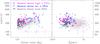 |
Fig. 5 Comparison between the structural and dynamical properties of ultramassive dense ETGs over the last ~10 Gyr. Magenta points indicate dense ETGs at 1.2 ≲ z< 1.6, open blue triangles indicate dense ETGs at 0.3 ≲ z ≲ 0.9, and local ETGs are shown with dark grey small dots. Light grey points are the whole sample of local ETGs with M⋆> 1011M⊙, thus with no cut in mean stellar mass density. Grey open squares indicate the local ultramassive dense galaxies selected from the sample of local galaxies with velocity dispersion >350 km s-1 by Bernardi et al. (2008), while open magenta circles show high-z ETGs evolved in size a factor ~3, as predicted by the relation ⟨ Re ⟩ ∝ (1 + z)-1.5and in σ according to the merger scenario by (Hopkins et al. 2009). In each panel, average error bars are reported. They are colour coded according to the sample they refer. For what concerns the high-z sample, we have found that on average δRe/Re ~ 11%, δσe/σe~10% (see Tables 3 and 4), while we have assumed a typical uncertainty of 20% on M⋆. At intermediate redshift, δRe/Re~10%, δσe/σe ~ 7%, and δM⋆ = 0.10 dex (see Saglia et al. 2010). In local Universe, δM⋆ = 0.07 dex (see Salim et al. 2007), δσe/σe ~ 10%, and we assume δRe/Re ~ 15%. For the error on local Re we refer to La Barbera et al. (2010) which derive the structural parameters of SDSS galaxies on SDSS images using 2DPHOT. In fact, the errors on parameters are expected to be mainly driven by the characteristics of the images, and not by the software and/or procedure used. |
In the left and right panels of Fig. 5 we plot the velocity dispersion of ultramassive dense ETGs as a function of stellar mass and effective radius, respectively. The first thing that we may note is that all of the ultramassive dense ETGs at high-z have an ultramassive dense counterpart in the local Universe with comparable structural and dynamical properties. Also the two most massive (M⋆ ≳ 3 × 10¹¹M⊙) and densest (Σ > 5000 M⊙ pc-2) high-z ETGs, whose parameters are offset with respect to the other high-z dense ETGs, have counterparts. Their counterparts can be found among the local ultramassive dense galaxies belonging to the sample of SDSS galaxies with σ> 350 km s-1 selected by Bernardi et al. (2008) (Fig. 5 open squares). Hence, Fig. 6 shows that in local Universe there are ultramassive dense ETGs with effective radii and velocity dispersions comparable to those of equally massive and dense ETGs at ⟨ z ⟩ = 1.4. At the same time, Fig. 5 shows that there are some local galaxies with σe< 200 km s-1 without high-z counterparts. These ETGs populate the region in Fig. 4 immediately below the line at Σ = 2500 M⊙ pc-2 with 1011<M⋆< 2 × 10¹¹, where indeed no high-z galaxies fall. Actually, the sparse sampling of the high-z sample and its incompleteness, prevent us from assesing whether the lack of low-σ ultramassive dense ETGs at high-z is real or not.
As an exercise, we show, with open circles in Fig. 5, the displacement that high-z dense ETGs would show in the space (Re, M⋆, σe) under the hypothesis that they evolve in size according to the relation (1 + z)-1.5 (i.e. a factor ~ 3 from z ~ 1.4 to z = 0, as found e.g. by Cassata et al. 2013; Cimatti et al. 2012; van der Wel et al. 2014), and in σ according to the merging scenario proposed by Hopkins et al. (2009). Thus, if all or most of the high-z ultramassive dense ETGs evolve in size (and σe), they have to be replaced by other ultramassive dense ETGs along the time to restore the population seen in the local Universe.
4. Discussion and conclusions
We have investigated the mass accretion history of ultramassive dense (M⋆> 1011M⊙, Σ > 2500 M⊙ pc-2) ETGs, elliptical and spheroidal galaxies selected on the basis of visual selected, over the last ~9 Gyr. We addressed this topic by tracing the evolution of their comoving number density and comparing the structural (effective radius Re and stellar mass M⋆) and dynamical (velocity dispersion σe) parameters of ultramassive dense ETGs from redshift ~1.6 to redshift ~0.
We took advantage of the MUNICS and GOODS-South surveys to constrain the comoving number density ρ of ultramassive dense ETGs since at 1 <z< 1.6, while we used the COSMOS spectroscopic survey to cover the redshift range from z = 1.0 to z = 0.2. For the number density of ultramassive dense ETGs in the local Universe, we referred to the sample of local ETGs selected from the SDSS DR4 by Thomas et al. (2010). We found that the comoving number density follows the relation ρ ∝ (1 + z)0.3 ± 0.8, i.e. it decreases at most by 25% since z = 1.6.
Our results are in good agreement with the other findings presented in literature (Carollo et al.2013; Damjanov et al. 2015; Cassata et al.2013; Valentinuzzi et al.2010; Bezanson et al.2013), with the only two exceptions concerning the estimates provided by Taylor et al. (2010a) at z ~ 0, and by van der Wel et al. (2014) at 0.2 <z< 1.5; in both cases our number densities are greater than those claimed by the authors. In the first case, we have shown that the main source of the observed discrepancy is in the different definition of Re used; semi-major axes SMe that were obtained fitting a de Vaucouleur profile in the Taylor investigation versus circularized Re that was obtained fitting a Sersic profile in our analysis. In the second case, we argue that the main reason for the drastic (~one order of magnitude) drop observed in the number density by van der Wel et al. (2014) can be ascribed to the procedure they adopted to derive the effective radius at 5000 Å and the usage of semi-major axis SMe.
We then investigated whether the ultramassive dense ETGs observed at high-z have a local counterpart, i.e. whether they are similar both in their structure (Re and M⋆) and kinematics (σe) to the low-z ETGs. To this aim, we collected a homogeneous sample of ultramassive dense ETGs at 1.2 <z< 1.6 with available Re, M⋆, and σe. We only included in our final catalogue the galaxies with clear elliptical morphology, effective radius derived in the F160W band fitting a Sersic profile, stellar masses estimated with BC03 models, and a Chabrier IMF. The request of available velocity dispersion restricts the sample to 11 ETGs. For four ETGs out of 11 (plus one at z = 1.91), we presented new unpublished VLT-FORS2 spectra and the measure of their velocity dispersions. For the intermediate redshift range (0.2 <z< 0.9), we refer to the sample of ETGs by Saglia et al. (2010) and to the sample of passive galaxies by Zahid et al. (2015), while as local reference we adopted the complete sample of local (0.063 <z< 0.1) ETGs selected from the SDSS DR4 by Thomas et al. (2010). The comparison in the plane [Re, M⋆, σe] shows that all of the ultramassive dense ETGs at z = 1.4 have a local counterpart with a similar velocity dispersion, stellar mass, and effective radius.
The two pieces of evidences above point towards two simple scenarios. In the last 9−10 Gyr, the vast majority (≳70%, according to the number density) of ultramassive dense ETGs passively age, leaving the bulk of the stellar mass, kinematics, and structure almost unchanged. In this case, the observed size growth of ultramassive ETGs has to be ascribed mostly to newborn larger ETGs. The other possibility is that a significant portion of high-z ultramassive dense ETGs migrate, through inside-out accretion, towards less dense systems, thereby sustaining the mean size growth of spheroidal galaxies. Concurrently, the emergence of new ultramassive dense ETGs at lower redshift maintains the number density at almost constant. We are not in the position to discriminate among the two possibilities, but some considerations deserve to be discussed.
A conventional approach to distinguish the real descendants from the newly formed spheroids (i.e. to discriminate among the two above scenarios) is to compare high redshift galaxies with old (on the basis of their luminosity weighted age LWA) low-z galaxies. However, this method does not take into account the evidence that despite the old global age, spheroidal galaxies often host very young stars (e.g. La Barbera et al. 2012). Although this population of young stars has a negligible weight in terms of total stellar mass (e.g. Tantalo & Chiosi 2004), these young stars can significantly lower the LWA. The direct consequence of this is that to select local descendants through a cut in LWA can exclude a portion of spheroidal galaxies already in place at z ~ 1.4. As a further complication, most of the methods used to infer galaxies age are limited by the age-metallicity degeneracy and by the possible presence of the dust.
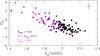 |
Fig. 6 The Hδ of ultramassive dense local ETGs versus their Dn(4000) colour coded on the basis of the 97.5 percentile value of F, where F is the fraction of stellar mass formed in the last 2 Gyr. |
Considering these aspects, we decided to investigate the distribution of local ultramassive dense ETGs in the Dn(4000) – Hδ plane. Actually, the Dn(4000) index progressively increases with the age of the stellar population, while the strong absorption Hδ line arises in galaxies that have experienced a burst of star formation in the past 1−2 Gyr. Although both indices are metallicity sensitive, their combination is not so and, moreover, is largely insensitive to the dust-attenuation effects. In Fig. 6 we reported the Dn(4000) and Hδ values for our sample of 124 ultramassive dense local ETGs. For the spectral indices we referred to the database provided by Kauffmann et al. (2003) for SDSS galaxies. The figure shows that just ~70% (60%) of local ultramassive dense ETGs have Dn(4000) ≳ 1.9(1.95) (thus age ≳9 Gyr), therefore, on the basis of their age, only two out of three local ETGs should be considered descendants of high-z compact ETGs. For each galaxy, however, Kauffmann et al. (2003) best fitted the observed values of Dn(4000) and Hδ with a grid of composite stellar population (CSP) models, which both had typical declining and bursty star formation history. From the best-fit model, they derived the fraction F of stellar mass formed in the last 2 Gyr and provided both its median value and the 2.5 and 97.5 percentile of its likelihood distribution. Actually, all of the galaxies in Fig. 6 have a median value of F = 0. However, in Fig. 6 we colour coded the galaxies on the basis of the 97.5 percentile value of F (F97.5). This is because beyond the exact value of F, which can be susceptible to the grid of the input models and prior adoption in the fit, we are interested in investigating whether there is a non-null probability to have a secondary (minor) event of star formation, which can drift the age estimate towards a lower value. Interestingly, in the vast majority of the galaxies with Dn(4000) ≳ 1.9 (and less than 10% for galaxies with Dn(4000) ≳ 1.95), F97.5 = 0. For the remaining galaxies of the sample with Dn(4000) < 1.9, their F97.5 value is > 0, thus there is a non-null probability that they experienced a burst of star formation in the last 2 Gyr. In this context, detailed studies on spectral features of passive galaxies (Lonoce et al. 2014) have shown that fitting the Dn(4000) with a single CSP model with a declining star formation history returns age values that can be significantly (even ≳50%) lower than the values obtained with a SED fitting or obtained assuming a composite model made by an old component forming the bulk of the stellar mass, and a young stellar population contributing just few % to the total stellar mass amount. If this is the case, the galaxies with Dn(4000) < 1.9 could be still considered descendant of high-z ETGs that experienced secondary and minor events of star formation at later epochs (see also Thomas et al. 2010). These events can have a drastic impact on the estimate of galaxy age, but do not significantly alter the stellar mass. Actually, Fig. 6 shows that the probability of a galaxy increasing its stellar mass by more than 20% in secondary events of star formation is extremely low.
This analysis is not intended to be quantitative, but to show that the treatment of the progenitor bias is very complex and that the mere selection of local descendants on the basis of the galaxy age that is obtained through the photometry fit or even through the more robust Dn(4000), can provide at most a lower limit to the true number of local descendants. A more detailed analysis of the whole ensemble of the spectral features that are age and “star-formation history” sensitive (e.g. Hδ; H+K, Dn(4000)) is mandatory both in local and at intermediate redshift range, to track the real mass assembly history of ETGs.
Although not conclusive, the analysis of spectral features of local ETGs have shown that there is a non-null probability that all of the local dense ETGs are high-z descendants. Moreover, in recent years, studies on the properties (number densities, masses, sizes, SFRs) of submillimeter galaxies (SMGs) have strengthened the possible evolutionary connection between these objects and dense high-z elliptical, in the direction that the SMGs are the progenitors of the dense ETGs (e.g. Barro et al. 2013, 2014; Toft et al. 2014). Nonetheless, these highly star-forming galaxies are extremely rare at z< 1. If galaxies with, for example, Dn(4000) < 1.9 are genuinely young ultradense systems (and not old galaxies that have experienced recent star-formation events), we should find a way to model their formation. The lack of progenitors for young dense ETGs, strengthens the hypothesis that local compact massive galaxies are descendants of high redshift galaxies.
Thus, more than one piece of observational evidence would point towards the first of the two proposed scenarios according to which most (≳75%) of the ultramassive dense ETGs observed at z ~ 1.4 have already completed their assembly. Although a residual event of star formation may occur, these cannot significantly modify neither the mass, the velocity dispersion, nor the typical dimension of the ultramassive dense galaxies already formed at z ~ 1.4. As far as the remaining 25% of dense ETGs possibly missing in the local Universe, stochastic merger events could have transformed them into non-dense systems (Σ ≤ 2500 M⊙ pc-2), contributing to the increase of the mean size and the number density of the whole population of ultramassive ETGs at z< 1.5. In fact, de la Rosa et al. (2016) have found that a portion of present-day massive galaxies host in the centre a compact core with the same structural and dynamical properties as high-z compact galaxies. Numerically, the contribution of these size-evolved ultramassive dense ETGs to the total number density of local ultramassive ETGs is ~2 × 10⁻⁵ gal/Mpc3 (see Fig. 2). Actually, the number density of passive M⋆>1011M⊙ galaxies increases from ~ 10-4 to 5 × 10⁻⁴ gal/Mpc-4 from redshift 1.5 to z ~ 0 (Ilbert et al. 2010; Pozzetti et al. 2010; Brammer et al. 2011; Moustakas et al. 2013; Muzzin et al. 2013). Therefore, if the fraction of newly formed ultramassive dense ETGs is negligible, the eventual contribution of the size-evolved ultramassive dense ETGs to the mean size growth in terms of number density is ≲5%.
The superscript 0.1 indicates rest-frame photometry redshifted to z = 0.1, (see, e.g., Blanton & Roweis 2007).
Acknowledgments
We warmly thank the anonymous referee for his/her comments and suggestions which, in our opinion, have really improved the whole manuscript. This work has received financial support from Prin-INAF 1.05.09.01.05 and is based on observations made with ESO Very Large Telescope under programme ID 085.A-0135A.
References
- Adelman-McCarthy, J. K., Agüeros, M. A., Allam, S. S., et al. 2006, ApJS, 162, 38 [NASA ADS] [CrossRef] [Google Scholar]
- Barro, G., Faber, S. M., Pérez-González, P. G., et al. 2013, ApJ, 765, 104 [NASA ADS] [CrossRef] [Google Scholar]
- Barro, G., Trump, J. R., Koo, D. C., et al. 2014, ApJ, 795, 145 [NASA ADS] [CrossRef] [Google Scholar]
- Belli, S., Newman, A. B., & Ellis, R. S. 2014, ApJ, 783, 117 [NASA ADS] [CrossRef] [Google Scholar]
- Bernardi, M. 2009, MNRAS, 395, 1491 [NASA ADS] [CrossRef] [Google Scholar]
- Bernardi, M., Hyde, J. B., Fritz, A., et al. 2008, MNRAS, 391, 1191 [NASA ADS] [CrossRef] [Google Scholar]
- Bezanson, R., van Dokkum, P. G., Tal, T., et al. 2009, ApJ, 697, 1290 [NASA ADS] [CrossRef] [Google Scholar]
- Bezanson, R., van Dokkum, P., & Franx, M. 2012, ApJ, 760, 62 [NASA ADS] [CrossRef] [Google Scholar]
- Bezanson, R., van Dokkum, P., van de Sande, J., Franx, M., & Kriek, M. 2013, ApJ, 764, L8 [NASA ADS] [CrossRef] [Google Scholar]
- Blanton, M. R., & Roweis, S. 2007, AJ, 133, 734 [NASA ADS] [CrossRef] [Google Scholar]
- Blanton, M. R., Schlegel, D. J., Strauss, M. A., et al. 2005, AJ, 129, 2562 [NASA ADS] [CrossRef] [Google Scholar]
- Brammer, G. B., Whitaker, K. E., van Dokkum, P. G., et al. 2011, ApJ, 739, 24 [NASA ADS] [CrossRef] [Google Scholar]
- Bruce, V. A., Dunlop, J. S., Cirasuolo, M., et al. 2012, MNRAS, 427, 1666 [NASA ADS] [CrossRef] [Google Scholar]
- Bruzual, G., & Charlot, S. 2003, MNRAS, 344, 1000 [NASA ADS] [CrossRef] [Google Scholar]
- Buitrago, F., Trujillo, I., Conselice, C. J., et al. 2008, ApJ, 687, L61 [NASA ADS] [CrossRef] [Google Scholar]
- Buitrago, F., Trujillo, I., Conselice, C. J., & Häußler, B. 2013, MNRAS, 428, 1460 [NASA ADS] [CrossRef] [Google Scholar]
- Calzetti, D., Armus, L., Bohlin, R. C., et al. 2000, ApJ, 533, 682 [NASA ADS] [CrossRef] [Google Scholar]
- Cappellari, M., & Emsellem, E. 2004, PASP, 116, 138 [NASA ADS] [CrossRef] [Google Scholar]
- Cappellari, M., Bacon, R., Bureau, M., et al. 2006, MNRAS, 366, 1126 [NASA ADS] [CrossRef] [Google Scholar]
- Cappellari, M., di Serego Alighieri, S., Cimatti, A., et al. 2009, ApJ, 704, L34 [NASA ADS] [CrossRef] [Google Scholar]
- Cappellari, M., Emsellem, E., Krajnović, D., et al. 2011, MNRAS, 413, 813 [NASA ADS] [CrossRef] [Google Scholar]
- Carollo, C. M., Bschorr, T. J., Renzini, A., et al. 2013, ApJ, 773, 112 [NASA ADS] [CrossRef] [Google Scholar]
- Carter, D., Goudfrooij, P., Mobasher, B., et al. 2008, ApJS, 176, 424 [NASA ADS] [CrossRef] [Google Scholar]
- Cassata, P., Giavalisco, M., Guo, Y., et al. 2011, ApJ, 743, 96 [NASA ADS] [CrossRef] [Google Scholar]
- Cassata, P., Giavalisco, M., Williams, C. C., et al. 2013, ApJ, 775, 106 [NASA ADS] [CrossRef] [Google Scholar]
- Chabrier, G. 2003, PASP, 115, 763 [NASA ADS] [CrossRef] [Google Scholar]
- Cimatti, A., Cassata, P., Pozzetti, L., et al. 2008, A&A, 482, 21 [NASA ADS] [CrossRef] [EDP Sciences] [Google Scholar]
- Cimatti, A., Nipoti, C., & Cassata, P. 2012, MNRAS, 422, L62 [NASA ADS] [CrossRef] [Google Scholar]
- Daddi, E., Renzini, A., Pirzkal, N., et al. 2005, ApJ, 626, 680 [NASA ADS] [CrossRef] [Google Scholar]
- Damjanov, I., McCarthy, P. J., Abraham, R. G., et al. 2009, ApJ, 695, 101 [NASA ADS] [CrossRef] [Google Scholar]
- Damjanov, I., Abraham, R. G., Glazebrook, K., et al. 2011, ApJ, 739, L44 [NASA ADS] [CrossRef] [Google Scholar]
- Damjanov, I., Hwang, H. S., Geller, M. J., & Chilingarian, I. 2014, ApJ, 793, 39 [NASA ADS] [CrossRef] [Google Scholar]
- Damjanov, I., Geller, M. J., Zahid, H. J., & Hwang, H. S. 2015, ApJ, 806, 158 [NASA ADS] [CrossRef] [Google Scholar]
- Davies, L. J. M., Driver, S. P., Robotham, A. S. G., et al. 2015, MNRAS, 447, 1014 [NASA ADS] [CrossRef] [Google Scholar]
- de la Rosa, I. G., La Barbera, F., Ferreras, I., et al. 2016, MNRAS, 457, 1916 [NASA ADS] [CrossRef] [Google Scholar]
- Drory, N., Feulner, G., Bender, R., et al. 2001, MNRAS, 325, 550 [NASA ADS] [CrossRef] [Google Scholar]
- Franx, M., van Dokkum, P. G., Schreiber, N. M. F., et al. 2008, ApJ, 688, 770 [NASA ADS] [CrossRef] [Google Scholar]
- Gargiulo, A., Saracco, P., Longhetti, M., La Barbera, F., & Tamburri, S. 2012, MNRAS, 425, 2698 [NASA ADS] [CrossRef] [Google Scholar]
- Giavalisco, M., Ferguson, H. C., Koekemoer, A. M., et al. 2004, ApJ, 600, L93 [NASA ADS] [CrossRef] [Google Scholar]
- Grogin, N. A., Kocevski, D. D., Faber, S. M., et al. 2011, ApJS, 197, 35 [NASA ADS] [CrossRef] [Google Scholar]
- Guo, Y., McIntosh, D. H., Mo, H. J., et al. 2009, MNRAS, 398, 1129 [NASA ADS] [CrossRef] [Google Scholar]
- Guo, Y., Giavalisco, M., Cassata, P., et al. 2011, ApJ, 735, 18 [NASA ADS] [CrossRef] [Google Scholar]
- Hopkins, P. F., Bundy, K., Murray, N., et al. 2009, MNRAS, 398, 898 [NASA ADS] [CrossRef] [Google Scholar]
- Hoyos, C., den Brok, M., Verdoes Kleijn, G., et al. 2011, MNRAS, 411, 2439 [NASA ADS] [CrossRef] [Google Scholar]
- Huertas-Company, M., Mei, S., Shankar, F., et al. 2013, MNRAS, 428, 1715 [NASA ADS] [CrossRef] [Google Scholar]
- Ilbert, O., Salvato, M., Le Floc’h, E., et al. 2010, ApJ, 709, 644 [NASA ADS] [CrossRef] [Google Scholar]
- Ilbert, O., McCracken, H. J., Le Fèvre, O., et al. 2013, A&A, 556, A55 [NASA ADS] [CrossRef] [EDP Sciences] [Google Scholar]
- Jorgensen, I., & Chiboucas, K. 2013, AJ, 145, 77 [NASA ADS] [CrossRef] [Google Scholar]
- Jorgensen, I., Chiboucas, K., Toft, S., et al. 2014, AJ, 148, 117 [NASA ADS] [CrossRef] [Google Scholar]
- Kauffmann, G., Heckman, T. M., White, S. D. M., et al. 2003, MNRAS, 341, 33 [NASA ADS] [CrossRef] [Google Scholar]
- Keating, S. K., Abraham, R. G., Schiavon, R., et al. 2015, ApJ, 798, 26 [NASA ADS] [CrossRef] [Google Scholar]
- Koekemoer, A. M., Aussel, H., Calzetti, D., et al. 2007, ApJS, 172, 196 [NASA ADS] [CrossRef] [Google Scholar]
- Koekemoer, A. M., Faber, S. M., Ferguson, H. C., et al. 2011, ApJS, 197, 36 [NASA ADS] [CrossRef] [Google Scholar]
- Kormendy, J. 1982, ApJ, 257, 75 [NASA ADS] [CrossRef] [Google Scholar]
- Kormendy, J., & Illingworth, G. 1982, ApJ, 256, 460 [NASA ADS] [CrossRef] [Google Scholar]
- Kroupa, P. 2001, MNRAS, 322, 231 [NASA ADS] [CrossRef] [Google Scholar]
- La Barbera, F., de Carvalho, R. R., de La Rosa, I. G., et al. 2010, MNRAS, 408, 1313 [NASA ADS] [CrossRef] [Google Scholar]
- La Barbera, F., Ferreras, I., de Carvalho, R. R., et al. 2012, MNRAS, 426, 2300 [NASA ADS] [CrossRef] [Google Scholar]
- Longhetti, M., Saracco, P., Severgnini, P., et al. 2007, MNRAS, 374, 614 [NASA ADS] [CrossRef] [Google Scholar]
- Longhetti, M., Saracco, P., Gargiulo, A., Tamburri, S., & Lonoce, I. 2014, MNRAS, 439, 3962 [NASA ADS] [CrossRef] [Google Scholar]
- Lonoce, I., Longhetti, M., Saracco, P., Gargiulo, A., & Tamburri, S. 2014, MNRAS, 444, 2048 [NASA ADS] [CrossRef] [Google Scholar]
- Mancini, C., Matute, I., Cimatti, A., et al. 2009, A&A, 500, 705 [NASA ADS] [CrossRef] [EDP Sciences] [Google Scholar]
- Mancini, C., Daddi, E., Renzini, A., et al. 2010, MNRAS, 401, 933 [NASA ADS] [CrossRef] [Google Scholar]
- Maraston, C., & Strömbäck, G. 2011, MNRAS, 418, 2785 [NASA ADS] [CrossRef] [Google Scholar]
- Marchesini, D., van Dokkum, P. G., Förster Schreiber, N. M., et al. 2009, ApJ, 701, 1765 [NASA ADS] [CrossRef] [Google Scholar]
- Moresco, M., Pozzetti, L., Cimatti, A., et al. 2013, A&A, 558, A61 [NASA ADS] [CrossRef] [EDP Sciences] [Google Scholar]
- Moustakas, J., Coil, A. L., Aird, J., et al. 2013, ApJ, 767, 50 [NASA ADS] [CrossRef] [Google Scholar]
- Munari, U., Sordo, R., Castelli, F., & Zwitter, T. 2005, A&A, 442, 1127 [NASA ADS] [CrossRef] [EDP Sciences] [Google Scholar]
- Muzzin, A., Marchesini, D., Stefanon, M., et al. 2013, ApJ, 777, 18 [NASA ADS] [CrossRef] [Google Scholar]
- Newman, A. B., Ellis, R. S., Treu, T., & Bundy, K. 2010, ApJ, 717, L103 [NASA ADS] [CrossRef] [Google Scholar]
- Newman, A. B., Ellis, R. S., Bundy, K., & Treu, T. 2012, ApJ, 746, 162 [NASA ADS] [CrossRef] [Google Scholar]
- Peng, C. Y., Ho, L. C., Impey, C. D., & Rix, H. 2002, AJ, 124, 266 [NASA ADS] [CrossRef] [Google Scholar]
- Poggianti, B. M., Calvi, R., Bindoni, D., et al. 2013a, ApJ, 762, 77 [NASA ADS] [CrossRef] [Google Scholar]
- Poggianti, B. M., Moretti, A., Calvi, R., et al. 2013b, ApJ, 777, 125 [NASA ADS] [CrossRef] [Google Scholar]
- Pozzetti, L., Bolzonella, M., Zucca, E., et al. 2010, A&A, 523, A13 [NASA ADS] [CrossRef] [EDP Sciences] [Google Scholar]
- Saglia, R. P., Sánchez-Blázquez, P., Bender, R., et al. 2010, A&A, 524, A6 [NASA ADS] [CrossRef] [EDP Sciences] [Google Scholar]
- Salim, S., Rich, R. M., Charlot, S., et al. 2007, ApJS, 173, 267 [NASA ADS] [CrossRef] [Google Scholar]
- Saracco, P., Longhetti, M., Severgnini, P., et al. 2005, MNRAS, 357, L40 [NASA ADS] [CrossRef] [Google Scholar]
- Saracco, P., Longhetti, M., & Andreon, S. 2009, MNRAS, 392, 718 [NASA ADS] [CrossRef] [Google Scholar]
- Saracco, P., Longhetti, M., & Gargiulo, A. 2010, MNRAS, L115 [Google Scholar]
- Saracco, P., Longhetti, M., & Gargiulo, A. 2011, MNRAS, 412, 2707 [NASA ADS] [CrossRef] [Google Scholar]
- Saracco, P., Casati, A., Gargiulo, A., et al. 2014, A&A, 567, A94 [NASA ADS] [CrossRef] [EDP Sciences] [Google Scholar]
- Sargent, M. T., Carollo, C. M., Lilly, S. J., et al. 2007, ApJS, 172, 434 [NASA ADS] [CrossRef] [Google Scholar]
- Scarlata, C., Carollo, C. M., Lilly, S., et al. 2007, ApJS, 172, 406 [NASA ADS] [CrossRef] [Google Scholar]
- Severgnini, P., Della Ceca, R., Braito, V., et al. 2005, A&A, 431, 87 [NASA ADS] [CrossRef] [EDP Sciences] [Google Scholar]
- Shen, S., Mo, H. J., White, S. D. M., et al. 2003, MNRAS, 343, 978 [NASA ADS] [CrossRef] [Google Scholar]
- Simard, L., Mendel, J. T., Patton, D. R., Ellison, S. L., & McConnachie, A. W. 2011, ApJS, 196, 11 [NASA ADS] [CrossRef] [Google Scholar]
- Stott, J. P., Collins, C. A., Burke, C., Hamilton-Morris, V., & Smith, G. P. 2011, MNRAS, 414, 445 [NASA ADS] [CrossRef] [Google Scholar]
- Strauss, M. A., Weinberg, D. H., Lupton, R. H., et al. 2002, AJ, 124, 1810 [NASA ADS] [CrossRef] [Google Scholar]
- Szomoru, D., Franx, M., Bouwens, R. J., et al. 2011, ApJ, 735, L22 [NASA ADS] [CrossRef] [Google Scholar]
- Szomoru, D., Franx, M., & van Dokkum, P. G. 2012, ApJ, 749, 121 [NASA ADS] [CrossRef] [Google Scholar]
- Tamburri, S., Saracco, P., Longhetti, M., et al. 2014, A&A, 570, A102 [NASA ADS] [CrossRef] [EDP Sciences] [Google Scholar]
- Tantalo, R., & Chiosi, C. 2004, MNRAS, 353, 405 [NASA ADS] [CrossRef] [Google Scholar]
- Taylor, E. N., Franx, M., Brinchmann, J., van der Wel, A., & van Dokkum, P. G. 2010a, ApJ, 722, 1 [NASA ADS] [CrossRef] [Google Scholar]
- Taylor, E. N., Franx, M., Glazebrook, K., et al. 2010b, ApJ, 720, 723 [NASA ADS] [CrossRef] [Google Scholar]
- Thomas, D., Maraston, C., Schawinski, K., Sarzi, M., & Silk, J. 2010, MNRAS, 404, 1775 [NASA ADS] [Google Scholar]
- Thomas, D., Steele, O., Maraston, C., et al. 2013, MNRAS, 431, 1383 [NASA ADS] [CrossRef] [Google Scholar]
- Toft, S., van Dokkum, P., Franx, M., et al. 2007, ApJ, 671, 285 [NASA ADS] [CrossRef] [MathSciNet] [Google Scholar]
- Toft, S., Smolčić, V., Magnelli, B., et al. 2014, ApJ, 782, 68 [NASA ADS] [CrossRef] [Google Scholar]
- Tortora, C., La Barbera, F., Napolitano, N. R., et al. 2016, MNRAS, 457, 2845 [NASA ADS] [CrossRef] [Google Scholar]
- Treu, T., Stiavelli, M., Møller, P., Casertano, S., & Bertin, G. 2001, MNRAS, 326, 221 [NASA ADS] [CrossRef] [Google Scholar]
- Trujillo, I., Feulner, G., Goranova, Y., et al. 2006, MNRAS, 373, L36 [NASA ADS] [CrossRef] [Google Scholar]
- Trujillo, I., Conselice, C. J., Bundy, K., et al. 2007, MNRAS, 382, 109 [NASA ADS] [CrossRef] [Google Scholar]
- Trujillo, I., Cenarro, A. J., de Lorenzo-Cáceres, A., et al. 2009, ApJ, 692, L118 [NASA ADS] [CrossRef] [Google Scholar]
- Valentinuzzi, T., Fritz, J., Poggianti, B. M., et al. 2010, ApJ, 712, 226 [NASA ADS] [CrossRef] [Google Scholar]
- van de Sande, J., Kriek, M., Franx, M., et al. 2013, ApJ, 771, 85 [NASA ADS] [CrossRef] [Google Scholar]
- van der Wel, A., Holden, B. P., Zirm, A. W., et al. 2008, ApJ, 688, 48 [NASA ADS] [CrossRef] [Google Scholar]
- van der Wel, A., Rix, H.-W., Wuyts, S., et al. 2011, ApJ, 730, 38 [NASA ADS] [CrossRef] [Google Scholar]
- van der Wel, A., Bell, E. F., Häussler, B., et al. 2012, ApJS, 203, 24 [NASA ADS] [CrossRef] [Google Scholar]
- van der Wel, A., Franx, M., van Dokkum, P. G., et al. 2014, ApJ, 788, 28 [NASA ADS] [CrossRef] [Google Scholar]
- van Dokkum, P. G., Franx, M., Kriek, M., et al. 2008, ApJ, 677, L5 [NASA ADS] [CrossRef] [Google Scholar]
- Wake, D. A., van Dokkum, P. G., & Franx, M. 2012, ApJ, 751, L44 [NASA ADS] [CrossRef] [Google Scholar]
- Windhorst, R. A., Cohen, S. H., Hathi, N. P., et al. 2011, ApJS, 193, 27 [NASA ADS] [CrossRef] [Google Scholar]
- Zahid, H. J., Damjanov, I., Geller, M. J., & Chilingarian, I. 2015, ApJ, 806, 122 [NASA ADS] [CrossRef] [Google Scholar]
- Zirm, A. W., van der Wel, A., Franx, M., et al. 2007, ApJ, 656, 66 [NASA ADS] [CrossRef] [Google Scholar]
Appendix A: Testing the reliability of Re and M⋆ for local SDSS ETGs
Appendix A.1: Effective radius of local SDSS ETGs
The effective radius for SDSS galaxies has been derived by many authors adopting different methods (e.g. a 1D fit with the NYU-VAC pipeline by Blanton et al. 2005; a 2D fit with GALFIT by Simard et al. 2011 and Guo et al. 2009) and it is not straightforward to assess which analysis provides the more accurate estimate of the parameter. In fact, all of these works have estimated the Re on SDSS images (PSF-FWHM = 1.4″ in r-band, pixel size = 0.396′′/px, i.e. ~0.56 kpc/px at z = 0.075), and thus the central region of the light profile (very sensitive to the Sersic index) of a typical ultramassive dense ETG is sampled by just 3−4 px in the redshift range we probed. Based on this evidence, to test the accuracy of the Re we used in this work, we compared the estimate of the effective radius derived by Blanton et al. (2005) from SDSS images, with those obtained using HST optical images (FWHM ≃ 0.12″, pixel size 0.05′′/px). We used the Canadian Astronomy Data Centre5 to find ACS-HST images in the F775W/F814W/F850LP/ filter for the 124 ultramassive dense ETGs of our sample, but, unfortunately, none of these ETGs has an HST optical counterpart.
Given this, we collected a sample of galaxies from literature that is included in the Blanton catalogue with Re estimated on HST images as well. We firstly refer to the COSMOS catalogue described in Sect. 2.2. In Fig. A.1 the Re of galaxies at 0.1 <z< 0.4 measured on HST/ACS-F814W images (~r-band rest frame) by Sargent et al. (2007) is reported versus the Re (r-band) taken from the Blanton release (blue points). The match between the two releases do not include galaxies with Re smaller than 2 kpc, hence, to investigate the reliability of Blanton estimates even at lower effective radii, we integrate the sample with galaxies taken from the ACS-Coma Cluster Survey (Carter et al. 2008). The effective radii of Coma galaxies were measured on the F814W images (exposure time ~1400 s) with GALFIT (Hoyos et al. 2011) and, in Fig. A.1, are compared with the i-band SDSS Re. The range of Re covered by the two samples (1 kpc ≲ Re ≲ 6 kpc) is very similar to that covered by our sample of ultramassive dense local ETGs. The figure shows that, in the range of radius of our ultramassive dense ETGs (1 kpc ≲ Re ≲ 6 kpc), the estimates by Blanton agree with those measured for HST images (Re,HTS = 1.03 ± 0.08Re,NY + 0.06 ± 0.24).
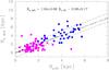 |
Fig. A.1 Effective radius measured on F814W/HST images for galaxies at 0.1 <z< 0.4 (blue points) and for galaxies in Coma cluster (magenta squares) compared with the estimates obtained on SDSS images by Blanton et al. (2005) in r-band, for galaxies at 0.1 <z< 0.4, and in i-band images for Coma galaxies. Solid line is the 1:1 correlation, long-dashed line is the best fit relation obtained with a sigma clipping algorithm, and dashed lines indicate the 1σ deviation from the best fit. |
Appendix A.2: Stellar mass of local SDSS ETGs
SDSS galaxies are provided with different estimates of stellar masses. In our analysis we decided to adopt the stellar masses derived through the SED fitting for consistency with high and intermediate redshift stellar mass estimates. To show that our conclusions are not affected by our choice of M⋆, in this Appendix we compare two different estimates of this quantity to asses the consistency of the measures, at least in the range of values we are interested in.
In the left panel of Fig. A.2 we plot the stellar mass derived through the fit of the multiband photometry (used in this paper, M⋆,photo) versus that obtained fitting the spectral indices (M⋆,index, Kauffmann et al. 2003).
The figure shows that for the bulk of local ETGs with M⋆,photo> 1011M⊙ the two estimates agree well, but a few percent of these significantly deviate from the main correlation. In the figure, we identified these outliers, represented in the figure by squares, as those galaxies at 3 sigma from the best-fit relation derived with a sigma clipping algorithm. We notice that a significant portion of outliers below the relation has M⋆,photo> 1011M⊙, while M⋆,index< 1011M⊙. Among these ultramassive outliers, we highlighted with open blue squares those with Σ > 2500 M⊙ pc-2, i.e. those included in the local sample of ultramassive dense local ETGs. To identify the more realistic stellar mass estimate for these ultramassive outliers, in the central panel we plot the velocity dispersion derived from the virial theorem (σvir) 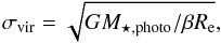 (A.1)where G is the gravitational constant and β = (8.87−0.831 × n + 0.0241 × n2), following Cappellari et al. (2006), versus the measured dispersion (σdr7). For the velocity dispersions of local ETGs, we used the DR7 σ; see Thomas et al. (2013) for more tests on the reliability of DR7 σ estimates.
The majority of ultramassive outliers deviate from the general trend and, in particular, at fixed σdr7, σvir should be lower. This suggests that the M⋆,photo for these galaxies are overestimated. As further confirmation, in the right panel we plot σdr7 versus σvir but with the last quantity derived from the M⋆,index estimates. We observe that in this case, the ultramassive outliers follow the main relation.
In fact, most of the ultramassive outliers despite having M⋆,photo> 1011M⊙, have M⋆< 1011M⊙ and thus we exclude them from our sample of local ultramassive dense ETGs.
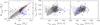 |
Fig. A.2 Left panel: stellar mass derived through the fit of the multiband photometry (used in this paper, M⋆,photo) vs. that obtained fitting the spectral indices (M⋆,index, Kauffmann et al. 2003) for local ETGs at 0.05 <z< 0.1 (light grey points). Black solid line is the 1:1 correlation, while red line is the best-fit relation and red-dotted curves are the 3σ lines. All of the points at >3σ are indicated as open squares. Among these outliers, blue squares are those with M⋆> 1011M⊙, and Σ > 2500 M⊙ pc-2, i.e. nominally included in local sample of ultramassive dense local ETGs. Dark grey points are the remaining part of the ultramassive dense local ETGs. Central panel: the measured velocity dispersion (σdr7) vs. the velocity dispersion derived from the virial theorem assuming the M⋆,photo values as mass (σvir,photo). Right panel: the same of central panel but with σvir derived assuming the M⋆,index values. |
Appendix B: Insights into the impact of Re definition on the samples of local dense galaxies
In Sect. 2.5.1, we have shown that the number of local massive dense galaxies is drastically dependent on the Re used. In particular, we have shown that in the spectroscopic SDSS-DR7 release, the number of galaxies with M⋆> 1011M⊙, log(Re/kpc) < 0.56 × (log(M⋆/M⊙) −9.84) −0.3, and 0.1(u−r) > 2.5 is ~10 if the semi-major axis obtained fitting a de Vaucouleur profile (SMe,dV) is used and increases up to ~190 if the circularized de Vaucouleur one (Re,dV) is used instead. Hereafter, for the sake of convenience, we refer to this last sample as the circularized sample. This implies that circularization (hence the axis ratio b/a) has a huge impact on the selection of the sample. In order to better visualize the impact of the b/a ratio on the selection of the sample, in the left panel of Fig. B.1 we plotted the galaxies of the circularized sample with reliable stellar mass (see Sect. 2.5.1) in the size-mass plane, using for each galaxy its semi-major axis SMe,dV. We colour coded the galaxies according to their b/a ratio. The solid line indicates the relation log(Re,dV/kpc) = 0.56 × (log(M⋆/M⊙) −9.84)−0.3.
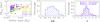 |
Fig. B.1 Left panel: sample of local dense galaxies selected using the Taylor et al.’s cuts and circularized de Vaucouleur radius Re,dV, and plotted in the size-mass plane using their semi-major de Vaucouleur axis SMe,dV. Galaxies are colour coded according to their b/a ratio, as declared in the labels. Solid line indicates the log(Re,dV/kpc) = 0.56 × (log(M⋆/M⊙) −9.84)−0.3 relation. Central panel: the distribution of the axis ratio b/a for the same galaxies in the left panel. Histogram counts are normalized to unity. Right panel: the distribution of the Sersic index n of local dense galaxies selected using the Taylor et al. cuts and circularized Sersic radius (blue histogram). Histogram counts are normalized to unity. Magenta histogram is the distribution of the Sersic index for our sample of ultramassive dense ETGs. |
As expected, the figure shows that ~10 galaxies have log(Re,dVnc/kpc) < 0.56×(log(M⋆/M⊙) −9.84)−0.3, while all of the others lie above the line with a b/a ratio that progressively decreases with the distance from the solid line, down to b/a ≃ 0.3. In the central panel of Fig. B.1, we reported the distribution of the axis ratio b/a for the same sample of galaxies. Half of the sample has b/a< 0.5 and this is the main reason for the drastic difference between the samples selected using circularized Re and semi-major axis SMe. The leftmost panel of Fig. B.1 also shows that only the galaxies with b/a ≳ 0.8−0.9 are included in both samples and this is the main reason why, even if our ultramassive dense ETGs are expected to be mostly roundish systems, i.e. objects for which their semi-major axes should be similar to their Re, Taylor et al. do not selected them in their sample. In fact, we have checked that only ~5% (six galaxies) of ETGs in our sample have b/a> 0.8, which are exactly those ETGs that satisfy the Taylor conditions.
Finally, in Sect. 2.5.1 we found that the number of local galaxies with M⋆> 1011M⊙, log(Re/kpc) < 0.56 × (log(M⋆/M⊙) −9.84)−0.3, 0.1(u−r) > 2.5 still increases if circularized Sersic Re are used (in particular, only ~45% of the galaxies are included in the sample selected using circularized de Vaucouleur Re). This result, as claimed in Sect. 2.5.1, is expected, because dense galaxies are known to have a Serisc index that is lower than 4. In the right panel of Fig. B.1 we reported the distribution of the Sersic index n for the local dense galaxies selected using the Taylor et al. cut and circularized Sersic Re: more than 80% of the galaxies have n< 4. There is also a tail of galaxies with a Sersic index that is lower than 2. This is mainly because galaxies are selected with a colour cut, and it is known that there is a non-negligible fraction of red disks. Actually, for comparison, the magenta histogram in the right panel of Fig. B.1 shows the distribution of the Sersic index for our sample of ultramassive dense ETGs. It is nice to observe how the tail at n< 2 disappears (no selection on the Sersic index is imposed a priori to the local sample of ETGs, or to any other sample used in our analysis), strengthening the robustness of the visual classification in selecting spheroidal galaxies.
Appendix C: The effect of the extrapolation on size measurements
In Sect. 2.5.3, we have shown that the extrapolation of the size of a galaxy via Eq. (2) by van der Wel et al. (2014) has an impact on the number of dense galaxies, therefore, in this Appendix, we aim to deepen the effect of the extrapolation on size measurements.
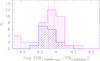 |
Fig. C.1 Distribution of the SMe,5000Å meas/SMe,5000Å der ratio as function of the redshift. SMRe,5000 Å meas is the semi-major axis at 5000 Å rest frame measured directly on the images, while SMe,5000Ådev is the same quantity, but inferred from F125W-band images using Eq. (2) from van der Wel et al. (2014). The blue histogram refers to ETGs at 0.5 <z< 0.7, while the magenta histogram refers to ETGs at 0.7 <z< 0.9. Solid lines are the median values of the distributions and dotted lines are the median value of the distribution at 25 and 75 percentile. |
In Fig. C.1, for the two bins of redshift 0.5 <z< 0.7, and 0.7 <z< 0.9, we reported the distribution of Log (SMe,5000Å meas/SMe,5000Å der) for a sample of elliptical galaxies, where SMe,5000Å meas is the semi-major axis at 5000 Å rest frame measured directly on images and SMe,5000Å der is that derived from SMe,F125W using Eq. (2) by van der Wel et al. (2014). For the galaxies at 0.5 <z< 0.7, we refer to a subsample of COSMOS ellipticals. More specifically, for the SMe,5000Å meas values we refer to the measurements by Sargent et al. (2007) on the F814W-band images and discussed in Sect. 2.2, while for the SMe,F125W values we considered the estimates by van der Wel et al. (2012). We crossmatched the two catalogues and selected only elliptical (ZEST-type = 1) galaxies with M⋆> 1010M⊙. For the galaxies at 0.7 <z< 0.9, we considered a sample of elliptical galaxies in the GOODS-South field. For the SMe,5000Å meas values, we used our sample of ETGs on GOODS-South (Tamburri et al. 2014) with the SMe derived from F850LP images (briefly described in Sect. 2.1), and for the SMe,F125W measurements we considered the catalogue by van der Wel et al. (2012). At 0.5 <z< 0.7, SMe,5000Å der overestimates the SMe,5000Å meas by a factor −0.08 dex (median value) and, in particular, for more than 80% of the galaxies SMe,5000Å meas/SMe,5000 Å der< 1. At 0.7 <z< 0.9, where the correction is extrapolated over a shorter wavelength range, this fraction decreases to ~65% and the median value is −0.02. The two samples of galaxies at 0.5 <z< 0.7 and 0.7 <z< 0.9 do not have exactly the same distribution in stellar mass and this can alter the relative comparison of their SMe,5000Å meas/SMe,5000Å der values. We checked, however, that the ratios SMe,F814W/SMe,F125W and SMe,F850LP/SMe,F125W do not depend on stellar mass, as stated by van der Wel et al. (2014). Although a test on more statistically significant samples would be necessary to be conclusive, Fig. C.1 shows that an average variation of SMe with λ (as assumed in the Eq. (2) by van der Wel) could not account for the variety of stellar populations in elliptical galaxies at high redshift (see e.g. Guo et al. 2011; Gargiulo et al. 2012), and this should be kept in mind in the analysis, interpretation and comparison of the results.
Appendix D: Velocity dispersion measurements at z ~ 1.4
Figure 3 shows the FORS2 spectra of the five galaxies of our high-z sample. As expected from the redshift estimates based on the continuum shape provided by AMICI spectra in the framework of the MUNICS survey, for the four galaxies at z ≲ 1.4 (ID 511, 633, 527, 389) we detected many absorption features (e.g. CN(3833 Å), the CaII K and H (3933+3968 Å), blue lines) in addition to the 4000 Å break. We notice that the ETG 527, whose elliptical morphology is confirmed by the HST image and surface brightness profile (see Fig. 1), clearly shows the O2 emission line at 3727 Å. We exclude that the presence of this emission line is due to AGN activity. In facts, the five ETGs of our sample were observed with XMM observations and only the source 443 has an X-ray detection (Severgnini et al. 2005). For galaxy 443, we detected the MgII absorption feature, as expected, however, we notice that the detection of this absorption line fixes the redshift of this galaxy at z = 1.91 which is slightly higher than the value originally estimated from the AMICI continuum (z = 1.70 ± 0.05). In Table 5 we report the values of the redshifts for the five galaxies of our sample.
The tool pPXF we adopted to derive the velocity dispersion describes the line-of-sight velocity distribution (LOSVD) as a Gauss+Hermite polynomial to take possible deviation of the line profile from a pure Gaussian shape into account. Following the prescription of the pPXF documentation, we ran simulations to define the value of the BIAS parameter, which is a penalty term that biases the solution towards a Gaussian shape if the higher moments of Hermite polynomial are not constrained from the data. We found that for our galaxies this term ranges between 0.1 and 0.2, which is in agreement with Cappellari et al. (2011).
Once we fixed the BIAS level, we measured the velocity dispersion by means of a weighted fit and adopted a set of synthetic stars as templates (see Sect. 3.1). To check for possible dependence of the σ estimate on the selected templates, we repeated the measure adopting a set of BC03 models with solar metallicity, τ = 0.1 Gyr, and varying age. We found that the σ values are perfectly comparable (differences <5%) with those obtained with the Munari stars. For clarity, the values reported in this paper and used in the analysis refer to σ estimates derived adopting the set of stars as templates.
We included in the fitting function both additive and multiplicative polynomials to take into account a possible residual template mismatch and eventual sky subtraction and spectral calibration errors. We verified the stability of our measures varying the degree (up to 6) of the two sets of polynomials and found that the detected variations in the estimates of velocity dispersion are lower than 3%, which is well within 1σ error bar.
Four out of five ETGs of our sample have spectra covering the rest-frame wavelength range ~[0.3−0.43] μm, thus including the 4000 Å break and many absorption features in addition to Ca H+K. In the past, several analyses have reported that the inclusion of the H+K features leads to an overestimate of the σ value, up to a factor of ~20% (Kormendy 1982; Kormendy & Illingworth 1982). These lines are intrinsically broad (~5 Å) and, in addition, the CaH line at 3968 Å is blended with Hϵ at 3969 Å. Moreover, error in fitting the steep continuum gradient at 4000 Å could produce a template mismatch. All of these factors can invalidate the measured dispersions. Nonetheless, the real impact of these feature on the σ estimates is not quantifiable a priori (e.g. Treu et al. 2001; van de Sande et al. 2013), thus we organized a set of simulations to test the reliability of our velocity dispersion measurements.
Briefly, for each galaxy of our sample, we created four model galaxy spectra starting from a simple stellar population model from Maraston & Strömbäck (2011) with solar metallicity and ages 2, 3, 4, 5 Gyr. We redshifted the spectra to the galaxy redshift, degraded them to the dispersion of real spectrum (~55 km s-1 per pixel), and added to them, pixel-by-pixel, a fake noise randomly extracted by the real noise. These template spectra were convoluted with a Gauss+Hermite LOSVD with the h3 and h4 Hermite moment equal to those measured on the real spectrum and velocity dispersion (σin) varying in the range ~[200−500] km s-1 over 500 steps. We fixed the line-of sight velocity V to zero. As an example, in Fig. D.1 we report a galaxy spectrum template that we constructed for the galaxy S2F1-633 with velocity dispersion 400 km s-1 (black line).
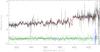 |
Fig. D.1 Example of the galaxy spectrum template (black line) we constructed for the real galaxy S2F1-633. The red line denotes the best-fit model, while the green points show the residuals. |
With the same star templates used on real spectra, we measured their velocity dispersions (σout), assuming a Gauss+Hermite polynomial as a fitting function. In Figs. D.2−D.5, and D.6 we present the results of the simulations for the galaxy S2F1-511, S2F1-633, S2F1-527, S2F1-389, S2F1-443.
The results we obtained show that, irrespective of the stellar population properties, for all of the galaxies of our sample, fitting a Gauss+Hermite polynomial over the whole wavelength range covered by our spectra, with a penalty BIAS ≃0.1, is the best choice to recover the intrinsic value of velocity dispersions. The same set of simulations for galaxy 443 shows the feasibility of extracting a reliable estimate of velocity dispersion from spectrum covering the blue wavelength range shortwards the 4000 Å in agreement with that found by Cappellari et al. (2009).
In fact, the difference, σout−σin, shows a slight offset that is always lower than the dispersion of the real spectrum (~55 km s-1 per pixel). The exact magnitude of the offset depends on the age and metallicity of the stellar population. We verified that the amount of the offset is not reduced excluding the region around the Ca H+K features from the fit, as done by Kormendy & Illingworth (1982); for this reason, we decided to include this part of the spectrum in our fit.
Moreover, our simulations have shown that for the σ we expect for our galaxies, the median value of the offset between σin and σout (σoff,median = σout−σin) depends on the age and metallicity of the input template, but is always smaller than the statistical error on measured velocity dispersion. In Table 5 we reported, for each galaxy, the minimum and maximum value of σoff,median we found in the six sets of simulations when σout is equal to the value we measured on real spectrum. The Table shows that the offset is never greater than 30 km s-1 and can be both positive and negative. Given these two aspects, and our uncertainty on stellar population properties, mostly on metallicity, we decided to not correct our measures for this offset, since we are not able to properly quantify its magnitude. Nonetheless, we note that our results would not change if we corrected the velocity dispersion of each galaxy for the maximum value of its offset.
The errors on velocity dispersion reported in Table 1 are the 25th and 75th percentile of the distributions of σoff estimated at σout equal to the velocity dispersion measured on real spectrum. Among the different set of simulations, the quoted errors are extracted from the simulation performed starting from a simple stellar population model with solar metallicity and age equal to that obtained from the fit of the observed SED. However, although the value of the offset is slightly dependent on the stellar population properties, its scatter not.
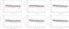 |
Fig. D.2 Top row: difference between the velocity dispersion measured (σout) and that provided as input (σin) in the model as function of σin for galaxy S2F1-511. The template adopted in the simulation have solar metallicity and age 2, 4, 5 Gyr from left to right. It is evident that the age of stellar populations do not affect our measurements. Bottom row: same as top row for the template with age 3 Gyr and subsolar, solar and super-solar metallicity from left to right. The three panels show that our uncertainty on stellar metallicity does not compromise our σ estimates. The red solid line is the median of the distribution, while the dashed lines are the 25th and 75th percentile. |
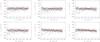 |
Fig. D.4 Same as Fig. D.2 for galaxy S2F1-527. Given the spectrum and SED fitting of this ETG, which both suggest a very young age for its stellar population, in the simulation of this galaxy we adopted, as galaxy templates, simple stellar population templates with solar metallicity and ages of 0.5, 1, 2 Gyr (upper panels, from left to right) and stellar population templates with an age of 3 Gyr and subsolar, solar, and super-solar metallicity (lower panels, from left to right). |
All Tables
Main characteristics of the surveys used to derived the number density evolution from z = 1.6 to z ~ 0.
Number density ρ of ultramassive dense (M⋆> 1011M⊙, Σ > 2500 M⊙ pc-2) ETGs from z = 1.6 to ~0.
All Figures
|
Fig. 1 Completeness of the spectroscopic SDSS galaxy catalogue with respect to the main galaxy sample as a function of galaxy Petrosian magnitude. |
| In the text | |
|
Fig. 2 Left: evolution of the comoving number density of ultramassive dense ETGs (M⋆ > 1011M⊙, Σ > 2500 M⊙ pc-2) from redshift 1.6 to redshift ~0 (blue symbols). The open blue square indicates the number density of ultramassive dense MUNICS ETGs at ⟨ z ⟩ = 1.4 corrected for the spectroscopic incompleteness of the MUNICS survey (see text). Solid blue line is the best-fit relation to our data in the range 0.066 < z < 1.6 (ρ ∝ (1 + z)0.3), while the blue dotted line indicates the mean value over the redshift range 0.066 < z < 1.6 (the dashed area indicates the 1σ deviation around this value). The orange squares indicate the number density for ultramassive compact galaxies by Damjanov et al. (2015), the magenta square by Trujillo et al. (2009), the light green square by Valentinuzzi et al. (2010), the purple squares by van der Wel et al. (2014), the salmon squares by Bezanson et al. (2009), the dark green square by Cassata et al. (2013), and the open red square by Taylor et al. (2010a). The points by Taylor et al. (open red square) and Cassata et al. (dark green square) are derived selecting from their sample only the galaxies with M⋆ > 1011M⊙ (see Table 3). The filled red square is the number density by Taylor et al. obtained using the circularized Sersic Re. Right: cuts in Re and M⋆ of our sample and other samples in the size to mass plane (colours are the same in the left panel). |
| In the text | |
|
Fig. 3 Left column: HST-NIC2/F160W images of the five ETGs of our high-z sample for which we present the VLT-FORS2 spectra (each image is 6×6 arcsec). Right column: spectra, unsmoothed and not-rebinned, of our five ETGs (black lines, 8 h of effective integration time). Many optical absorption features (blue lines) are clearly distinguishable from the continuum. The best-fit pPXF model is plotted in red. On average, pPXF selects and combines 2−4 star templates to reproduce the observed spectrum. Residuals after best-fit model subtraction are shown with green points. In the residual tracks, blue lines are the regions automatically excluded by the software pPXF as strongly affected by sky emission lines. |
| In the text | |
|
Fig. 4 Distribution of the ultramassive dense ETGs from z ~ 1.6 to z ~ 0 in the Re–M⋆ plane. Ultramassive dense ETGs at 1.2 <z< 1.6 are represented with magenta filled circles. The ETGs from MUNICS sample with available velocity dispersion (five presented here and one in Longhetti et al. 2014) are indicated with black countours. The ETG of MUNICS sample at redshift 1.91 (hence not included in the analysis of Sect. 3.3) is indicated with a blue point. Ultramassive dense ETGs at 0.3 <z< 0.9 and in the local Universe are indicated with blue open triangles and dark grey points, respectively. Solid black lines define the cuts in M⋆ and Σ of our samples. The small open circles show local ETGs from Thomas et al. (2010) in the redshift range 0.063 <z< 0.1. The red line indicates a line of constant σ derived as |
| In the text | |
|
Fig. 5 Comparison between the structural and dynamical properties of ultramassive dense ETGs over the last ~10 Gyr. Magenta points indicate dense ETGs at 1.2 ≲ z< 1.6, open blue triangles indicate dense ETGs at 0.3 ≲ z ≲ 0.9, and local ETGs are shown with dark grey small dots. Light grey points are the whole sample of local ETGs with M⋆> 1011M⊙, thus with no cut in mean stellar mass density. Grey open squares indicate the local ultramassive dense galaxies selected from the sample of local galaxies with velocity dispersion >350 km s-1 by Bernardi et al. (2008), while open magenta circles show high-z ETGs evolved in size a factor ~3, as predicted by the relation ⟨ Re ⟩ ∝ (1 + z)-1.5and in σ according to the merger scenario by (Hopkins et al. 2009). In each panel, average error bars are reported. They are colour coded according to the sample they refer. For what concerns the high-z sample, we have found that on average δRe/Re ~ 11%, δσe/σe~10% (see Tables 3 and 4), while we have assumed a typical uncertainty of 20% on M⋆. At intermediate redshift, δRe/Re~10%, δσe/σe ~ 7%, and δM⋆ = 0.10 dex (see Saglia et al. 2010). In local Universe, δM⋆ = 0.07 dex (see Salim et al. 2007), δσe/σe ~ 10%, and we assume δRe/Re ~ 15%. For the error on local Re we refer to La Barbera et al. (2010) which derive the structural parameters of SDSS galaxies on SDSS images using 2DPHOT. In fact, the errors on parameters are expected to be mainly driven by the characteristics of the images, and not by the software and/or procedure used. |
| In the text | |
|
Fig. 6 The Hδ of ultramassive dense local ETGs versus their Dn(4000) colour coded on the basis of the 97.5 percentile value of F, where F is the fraction of stellar mass formed in the last 2 Gyr. |
| In the text | |
|
Fig. A.1 Effective radius measured on F814W/HST images for galaxies at 0.1 <z< 0.4 (blue points) and for galaxies in Coma cluster (magenta squares) compared with the estimates obtained on SDSS images by Blanton et al. (2005) in r-band, for galaxies at 0.1 <z< 0.4, and in i-band images for Coma galaxies. Solid line is the 1:1 correlation, long-dashed line is the best fit relation obtained with a sigma clipping algorithm, and dashed lines indicate the 1σ deviation from the best fit. |
| In the text | |
|
Fig. A.2 Left panel: stellar mass derived through the fit of the multiband photometry (used in this paper, M⋆,photo) vs. that obtained fitting the spectral indices (M⋆,index, Kauffmann et al. 2003) for local ETGs at 0.05 <z< 0.1 (light grey points). Black solid line is the 1:1 correlation, while red line is the best-fit relation and red-dotted curves are the 3σ lines. All of the points at >3σ are indicated as open squares. Among these outliers, blue squares are those with M⋆> 1011M⊙, and Σ > 2500 M⊙ pc-2, i.e. nominally included in local sample of ultramassive dense local ETGs. Dark grey points are the remaining part of the ultramassive dense local ETGs. Central panel: the measured velocity dispersion (σdr7) vs. the velocity dispersion derived from the virial theorem assuming the M⋆,photo values as mass (σvir,photo). Right panel: the same of central panel but with σvir derived assuming the M⋆,index values. |
| In the text | |
|
Fig. B.1 Left panel: sample of local dense galaxies selected using the Taylor et al.’s cuts and circularized de Vaucouleur radius Re,dV, and plotted in the size-mass plane using their semi-major de Vaucouleur axis SMe,dV. Galaxies are colour coded according to their b/a ratio, as declared in the labels. Solid line indicates the log(Re,dV/kpc) = 0.56 × (log(M⋆/M⊙) −9.84)−0.3 relation. Central panel: the distribution of the axis ratio b/a for the same galaxies in the left panel. Histogram counts are normalized to unity. Right panel: the distribution of the Sersic index n of local dense galaxies selected using the Taylor et al. cuts and circularized Sersic radius (blue histogram). Histogram counts are normalized to unity. Magenta histogram is the distribution of the Sersic index for our sample of ultramassive dense ETGs. |
| In the text | |
|
Fig. C.1 Distribution of the SMe,5000Å meas/SMe,5000Å der ratio as function of the redshift. SMRe,5000 Å meas is the semi-major axis at 5000 Å rest frame measured directly on the images, while SMe,5000Ådev is the same quantity, but inferred from F125W-band images using Eq. (2) from van der Wel et al. (2014). The blue histogram refers to ETGs at 0.5 <z< 0.7, while the magenta histogram refers to ETGs at 0.7 <z< 0.9. Solid lines are the median values of the distributions and dotted lines are the median value of the distribution at 25 and 75 percentile. |
| In the text | |
|
Fig. D.1 Example of the galaxy spectrum template (black line) we constructed for the real galaxy S2F1-633. The red line denotes the best-fit model, while the green points show the residuals. |
| In the text | |
|
Fig. D.2 Top row: difference between the velocity dispersion measured (σout) and that provided as input (σin) in the model as function of σin for galaxy S2F1-511. The template adopted in the simulation have solar metallicity and age 2, 4, 5 Gyr from left to right. It is evident that the age of stellar populations do not affect our measurements. Bottom row: same as top row for the template with age 3 Gyr and subsolar, solar and super-solar metallicity from left to right. The three panels show that our uncertainty on stellar metallicity does not compromise our σ estimates. The red solid line is the median of the distribution, while the dashed lines are the 25th and 75th percentile. |
| In the text | |
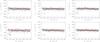 |
Fig. D.3 Same as Fig. D.2 for galaxy S2F1-633. |
| In the text | |
|
Fig. D.4 Same as Fig. D.2 for galaxy S2F1-527. Given the spectrum and SED fitting of this ETG, which both suggest a very young age for its stellar population, in the simulation of this galaxy we adopted, as galaxy templates, simple stellar population templates with solar metallicity and ages of 0.5, 1, 2 Gyr (upper panels, from left to right) and stellar population templates with an age of 3 Gyr and subsolar, solar, and super-solar metallicity (lower panels, from left to right). |
| In the text | |
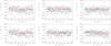 |
Fig. D.5 Same as Fig. D.2 for galaxy S2F1-389. |
| In the text | |
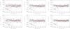 |
Fig. D.6 Same as Fig. D.2 for galaxy S2F1-443. |
| In the text | |
Current usage metrics show cumulative count of Article Views (full-text article views including HTML views, PDF and ePub downloads, according to the available data) and Abstracts Views on Vision4Press platform.
Data correspond to usage on the plateform after 2015. The current usage metrics is available 48-96 hours after online publication and is updated daily on week days.
Initial download of the metrics may take a while.