| Issue |
A&A
Volume 591, July 2016
|
|
|---|---|---|
| Article Number | A30 | |
| Number of page(s) | 17 | |
| Section | Astrophysical processes | |
| DOI | https://doi.org/10.1051/0004-6361/201527981 | |
| Published online | 07 June 2016 | |
Formation of a protocluster: A virialized structure from gravoturbulent collapse
I. Simulation of cluster formation in a collapsing molecular cloud
1
Laboratoire AIM, Paris-Saclay, CEA/IRFU/SAp – CNRS – Université Paris
Diderot,
91191
Gif-sur-Yvette Cedex,
France
e-mail:
yueh-ning.lee@cea.fr
2
LERMA (UMR CNRS 8112), École Normale Supérieure, 75231
Paris Cedex,
France
e-mail:
patrick.hennebelle@lra.ens.fr
Received: 16 December 2015
Accepted: 25 March 2016
Context. Stars are often observed to form in clusters and it is therefore important to understand how such a region of concentrated mass is assembled out of the diffuse medium. The properties of such a region eventually prescribe the important physical mechanisms and determine the characteristics of the stellar cluster.
Aims. We study the formation of a gaseous protocluster inside a molecular cloud and associate its internal properties with those of the parent cloud by varying the level of the initial turbulence of the cloud with a view to better characterize the subsequent stellar cluster formation.
Methods. We performed high resolution magnetohydrodynamic (MHD) simulations of gaseous protoclusters forming in molecular clouds collapsing under self-gravity. We determined ellipsoidal cluster regions via gas kinematics and sink particle distribution, permitting us to determine the mass, size, and aspect ratio of the cluster. We studied the cluster properties, such as kinetic and gravitational energy, and made links to the parent cloud.
Results. The gaseous protocluster is formed out of global collapse of a molecular cloud and has non-negligible rotation owing to angular momentum conservation during the collapse of the object. Most of the star formation occurs in this region, which occupies only a small volume fraction of the whole cloud. This dense entity is a result of the interplay between turbulence and gravity. We identify such regions in simulations and compare the gas and sink particles to observed star-forming clumps and embedded clusters, respectively. The gaseous protocluster inferred from simulation results presents a mass-size relation that is compatible with observations. We stress that the stellar cluster radius, although clearly correlated with the gas cluster radius, depends sensitively on its definition. Energy analysis is performed to confirm that the gaseous protocluster is a product of gravoturbulent reprocessing and that the support of turbulent and rotational energy against self-gravity yields a state of global virial equilibrium, although collapse is occurring at a smaller scale and the cluster is actively forming stars. This object then serves as the antecedent of the stellar cluster, to which the energy properties are passed on.
Conclusions. The gaseous protocluster properties are determined by the parent cloud out of which it forms, while the gas is indeed reprocessed and constitutes a star-forming environment that is different from that of the parent cloud.
Key words: standards / stars: formation / ISM: clouds / open clusters and associations: general / turbulence
© ESO, 2016
1. Introduction
An essential step to the understanding of how and in which conditions stars form is to unveil the process through which the dense prestellar cores collapse from molecular clouds. In terms of density, this process implies a change of more than ten orders of magnitude. To reduce the complexity, the study of star formation is often decomposed into hierarchical steps. Stars are frequently observed to be born in clusters and many studies stress the importance of understanding star formation in this context (Lada & Lada 2003; Longmore et al. 2014). In this work, we focus on the formation of a gaseous protocluster, the primary stage of cluster formation, that is to say the phase during which it assembles its gas and converts it into stars, with a view to better characterize the star formation environment and to prescribe more precisely the physical mechanisms at play.
The catalog reported by Lada & Lada (2003) for embedded clusters is consistent with the mass-size relation R ~ M1/3 − M1/2 for low-mass clusters as pointed out by Murray (2009), where R and M are the gas radius and mass, respectively. While the stellar mass of an embedded cluster is not directly observable and is obtained by assuming an underlying universal initial mass function (IMF), Adams et al. (2006) compiled data from Lada & Lada (2003) and Carpenter (2000) and showed a number-size relation  between the radius of the cluster and the number of objects it contains. The results of Gutermuth et al. (2009) are also compatible with this relation. The number-size relation is reasonably equivalent to the mass-size relation if we adopt a universal IMF and thus similar averaged mass among clusters. Despite the slight uncertainty in the power-law exponent, varying from 1/3 to 1/2, and the scatter of the data, it is clear that embedded clusters follow some mass-size relation. Larger data sets of star-forming clumps, identified as gaseous protoclusters, also exhibit a mass-size relation. Fall et al. (2010) compiled the observations of Shirley et al. (2003), Faúndez et al. (2004), and Fontani et al. (2005) in their Fig. 1, and found via least-squares regression the relation R ∝ M0.38. A regression fit on the ATLASGAL survey (Urquhart et al. 2014) data gives a dependence of R ∝ M0.50. In their work, they fitted log (M) to log (R) and found M ∝ R1.67, of which the power-law exponent is not the inverse of what we inferred. This indicates that the clump properties are differently dispersed in size and mass, and thus there exist some uncertainties in the power-law dependence. Meanwhile, both studies exhibit mass scatter of about 1 dex and are compatible with constant gas surface density, that is, R ∝ M0.5. These observations are performed with molecular lines and dust continuum of the star-forming gas, suggesting that the mass-size relation and probably some other properties of the stellar cluster are established as early as the gas-dominated phase. Pfalzner et al. (2016) pointed out that the mass-size relation for embedded clusters and gaseous protoclusters follow the same trend with different absolute value, which could be explained with star formation efficiency or cluster expansion. One interesting question to ask would be what physical processes actually determine this mass-size relation. Its existence suggests that this primary phase of cluster formation, the gaseous protocluster, is very likely in some equilibrium state governed by the molecular cloud environment in which it resides, and is crucial for understanding the nature of the cluster and, more generally, star formation. An analytical study by Hennebelle (2012) yielded, by linking the gaseous protocluster to properties of the parent cloud, R ~ M1/3 or R ~ M1/2 for protoclusters with different accretion schemes. We stress that we are emphasizing a global equilibrium, which does not imply that the structure is not locally collapsing. More precisely, we propose that the large scales are supported by a combination of rotation and turbulence that sets the M-R relation.
Many numerical studies of star or core formation inside molecular clouds have been performed to understand the impact of turbulence and gravity on star formation and the origin of the IMF. For example, studies such as Padoan et al. (2007) and Schmidt et al. (2010) looked for gravitationally unstable clumps inside hydrodynamic or magnetohydrodynamic (MHD) simulations of a piece of molecular cloud to produce a mass spectrum and compared to theories. Girichidis et al. (2011, 2012) compared the clusters formed in 100 M⊙ clouds with various initial density profiles and types of turbulence using adaptive mesh refinement (AMR) hydrodynamical simulations. Klessen et al. (1998) and Klessen & Burkert (2000) simulated a piece of clumpy molecular cloud with periodic boundary conditions initialized with Gaussian random field using the smoothed particle hydrodynamics (SPH) method. These authors identified cores forming in clusters. Bonnell et al. (2003), Bonnell et al. (2008), and Smith et al. (2009) performed hydrodynamical SPH simulations of 103 M⊙ uniform density spherical isothermal clouds and 104 M⊙ cylindrical clouds with a gradient in density, respectively. These authors followed star formation with sink particles and focused on the hierarchical process of cluster formation from the merging of subclusters. They stressed the important role of interactions among stars and of gravitational potential created by the cluster on the formation of brown dwarfs. Ballesteros-Paredes et al. (2015) used SPH to simulate a 103 M⊙ cloud to characterize the impact of self-gravity on the high-mass end slope of the IMF. To study the transition from cloud to stellar cluster and the link between their properties and, in particular, the later evolution of stellar clusters, Moeckel & Bate (2010) and Fujii & Portegies Zwart (2015) performed SPH simulations of a molecular cloud for one free-fall time, converted the dense gas to stars, and then evolved with N-body simulations to form clusters. These studies do not explicitly address in great detail how the gas, which is converted into clustered stars, is assembled and whether and how the properties of the stellar clusters are inherited from the gas phase.
In this paper, we focus on understanding the gas-dominated phase of early cluster formation inside molecular clouds, and show that the properties of the gaseous protocluster are determined by those of its parent cloud and are subsequently inherited by the stellar cluster. We focus on the transition between the global collapse that takes place at larger scales and the mechanical equilibrium at smaller scales, creating the gaseous protocluster. An energy equilibrium is reached for this gas-dominated object through gravoturbulent interaction, and its high density provides a favorable environment for star formation. Certain characteristics of the stellar cluster are therefore determined at the gas-dominated phase.
More precisely, this work aims to characterize the gaseous protocluster formed in molecular clouds collapsing under self-gravity. We perform a series of simulations of gaseous protocluster formation inside a molecular cloud for various levels of initial turbulent support. We identify such gaseous protocluster regions and analyze their properties to examine whether these structures are indeed objects in equilibrium and if they coincide with observations of star-forming clumps. We also discuss the sink particles forming therein and compare the sink cluster with observations of embedded clusters. Once the nature of the clusters is known, we can thus investigate star formation given this recipe of a cluster environment to gain knowledge of the star formation rate, the star-forming mechanisms, the initial mass function, etc. From a numerical point of view, the wide range of temporal and spatial scales concerned in star formation simulations have always been computationally challenging. The knowledge of how a gaseous protocluster forms in a molecular cloud could serve as a valuable tool for initializing a more realistic star formation simulation without having to include the whole cloud into the simulation box, and thus could help gain computation time or resolution.
To better understand the simulation results, an analytical model is introduced in the companion paper (Paper II) to account for the gaseous protocluster formation in a collapsing molecular cloud, which reaches quasi-stationary equilibrium. Similar ideas following Hennebelle (2012) are used to derive the virial equilibrium for an accreting system. As a natural consequence of angular momentum conservation during collapse, rotation is seen in observations (Hénault-Brunet et al. 2012; Davies et al. 2011; Mackey et al. 2013) and simulations. The system is therefore no longer spherically symmetric and we decompose the energy equilibrium of the protocluster into two dimensions. This model provides a link from cloud properties to that of the cluster and determines the cluster mass, size, velocity dispersion, and rotation. The mass-size relation inferred from observations (Fall et al. 2010; Urquhart et al. 2014) is very closely reproduced, provided that the parent molecular cloud is initially in a state close to virial equilibrium.
The paper is organized as follows. We first describe in Sect. 2 how the simulations are performed to investigate protocluster formation in molecular clouds. In Sect. 3, we explore different methods for identifying the cluster in the simulation results. Both gas kinematics and sink particle distribution are considered. The results are compared to observational measurements. The energy equilibrium and internal properties of the protocluster are discussed in Sect. 4. Finally, we make some remarks and conclusions in Sect. 5.
2. Simulations
We perform numerical simulations of a collapsing molecular cloud under self-gravity with the MHD AMR code RAMSES (Teyssier 2002; Fromang et al. 2006), which uses a Godunov’s scheme and constrained transport method to ensure null magnetic field divergence. We first introduce the initial conditions of the cloud and physical processes considered. We also give numerical details of the simulations and some qualitative results are presented at the end.
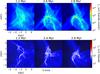 |
Fig. 1 Zoomed images of run B at times 1.2, 2.4, and 2.8 Myr, showing the central dense objet. Upper panel: column density. Lower panel: velocity field overplotted on density sliced map. The origin of the coordinate corresponds to the center of the computational box and the figures are recentered such that the densest cell in the rightmost panel is at the center of the image. Sink particles are not shown. |
2.1. Physical processes and initial condition
The evolution of the cloud is governed by ideal MHD equations with a cooling function of the ISM considered, as that described by Audit & Hennebelle (2005).
A series of molecular clouds with different levels of initial turbulence are performed. Simulations are initialized with a Bonnor-Ebert-like spherical cloud of 104 solar mass that has a density profile ![\hbox{$\rho(r) = \rho_0 /\left[ 1+\left({r \over r_0}\right)^2\right]$}](/articles/aa/full_html/2016/07/aa27981-15/aa27981-15-eq20.png) with ten times density contrast between the center and the edge, where ρ0 = 822 H cc-1 and r0 = 2.5 pc. The cloud has 15 pc diameter and the computational box is twice the size of the cloud, i.e., 30 pc in each dimension. The space surrounding the cloud is patched with diffuse gas of uniform density ρ0/ 100. The initial temperature is set by the cooling function and it is about 10 K in the dense gas. A turbulent velocity field is generated with a Kolmogorov spectrum with random phase and is scaled in such a way that the initial Mach numbers are 2.7, 6, 7.3, and 10, respectively. A weak magnetic field with uniform mass-to-flux ratio in the x direction is applied. Its highest value is about 8 μG at the cloud center and reaches about 3 μG at the cloud edge.
with ten times density contrast between the center and the edge, where ρ0 = 822 H cc-1 and r0 = 2.5 pc. The cloud has 15 pc diameter and the computational box is twice the size of the cloud, i.e., 30 pc in each dimension. The space surrounding the cloud is patched with diffuse gas of uniform density ρ0/ 100. The initial temperature is set by the cooling function and it is about 10 K in the dense gas. A turbulent velocity field is generated with a Kolmogorov spectrum with random phase and is scaled in such a way that the initial Mach numbers are 2.7, 6, 7.3, and 10, respectively. A weak magnetic field with uniform mass-to-flux ratio in the x direction is applied. Its highest value is about 8 μG at the cloud center and reaches about 3 μG at the cloud edge.
The ratios of characteristic timescales at the central plateau region (r<r0) are used as parameters to specify the initial conditions. In all runs, we use the ratio of free-fall time to sound crossing time tff/tsct = 0.15, and the ratio of free-fall time to Alfvén crossing time tff/tact = 0.2, which corresponds to a value of the mass-to-flux over critical mass-to-flux ratio of about 8. This implies that both thermal and magnetic energy are small compared to the gravitational potential energy. The ratio between free-fall time and turbulent crossing time tff/tvct is varied in each run, giving different levels of kinetic support against self-gravity. In Table 1, we provide the values of tff/tvct and the corresponding turbulent rms velocity, Mach number, and virial parameter αvir = 2Ekin/Egrav to characterize the initial energy state of the molecular cloud.
Simulation parameters: the cloud is specified with varying level of the ratio tff/tvct.
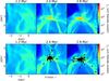 |
Fig. 2 Zoomed images of run B at times 1.2, 2.4, and 2.8 Myr. Upper panel: column density. Lower panel: sink particles overplotted on column density. The circles represent the sink particles with the size proportional to the log of their masses and the arrows indicate their velocity. |
2.2. Numerical setup
We start with a 1283 base grid and allow seven levels of refinement (equivalent to 163843) using an AMR scheme to ensure a resolution of ten grids per jeans length. When increasing by one level, a cell is subdivided into two in each dimension. This gives a resolution of 0.23 pc on the coarse grids and refinement down to 0.002 pc (or 400 AU) at the densest regions. Neumann boundary conditions with imposed zero gradients are used, which allows the gas to outflow from the computational box.
Sink particles are used in our simulations, as described by Bleuler & Teyssier (2014), and the densest region unresolved with a fluid description is replaced with a sink particle to economize computational power and to follow accretion onto Lagrangian mass. These particles are formed when density exceeds 108 H cc-1, while the flow is convergent and super-virial. The sink radius is equal to four computational cells at the finest resolution. After their formation, the sink particles are capable of accreting mass from their surrounding. As these high density regions represent possible star formation sites, they furnish dynamical and statistical hints on stellar cluster properties. We caution that although our resolution is very small with respect to the cluster size, ensuring good description of the cluster itself, the sink particle size is too large for the sinks to represent individual stars. The typical mass of our sink particles is on the order of ≃10 M⊙.
2.3. Qualitative presentations
Column density maps and velocity field overplotted on density slice maps are shown in Fig. 1 for run B. Figures 2 and 3 show a zoomed view of the central region where the protocluster is forming. The cloud is globally collapsing, while filamentary structures are forming under gravoturbulent interactions. When zooming in toward the central region, we see a parsec-scale prominent entity of relatively high density emerging, whose size is slowly varying in time. A general rotational motion becomes evident as the collapse proceeds, since there is no dissipative mechanism at this scale that is efficient enough to remove a large amount of angular momentum. The global infalling motion is noticeably reduced upon striking the central objet, forming highly irregular shocks at the seemingly ill-defined border.
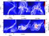 |
Fig. 3 Zoomed images of run B at times 1.2, 2.4, and 2.8 Myr focusing on the central dense objet with two views showing the flattened shape. Upper panel: velocity field overplotted on density sliced map, edge-on view. Lower panel: velocity field overplotted on density sliced map, face-on view of the flattened rotating protocluster. |
To have a fully physical description of a realistic self-regulation of star mass accretion and cluster formation, stellar feedbacks such as radiations (Bate 2009, 2012; Price & Bate 2009; Commerçon et al. 2011; Krumholz et al. 2012), protostellar jets and outflows (Wang et al. 2010; Nakamura & Li 2011, 2014; Dale et al. 2013c, 2015; Federrath et al. 2014; Federrath 2015), HII regions (Krumholz et al. 2007; Peters et al. 2010; Dale et al. 2013a,b, 2015; Geen et al. 2015), and supernovae (Iffrig & Hennebelle 2015; Walch & Naab 2015) should be incorporated. We limit ourselves to the simple scenario without feedback mechanisms, in which nothing except the depletion of cloud gas can stop sink accretion. We therefore stop the simulations when about half of the initial cloud mass has been accreted onto the sink particles, since the results are less likely to be physical in this stage. This corresponds to physical time of about three million years. While some of the sink particles form in the filamentary structures feeding the central cluster, most of the sinks are observed to form within the gaseous protocluster, hence strongly suggesting that this central region is an important site for understanding star properties such as the IMF.
3. Inferring the protocluster radius from simulation results
As previously depicted, although a prominent structure forming at the center of the cloud is exhibited, it is indeed highly irregular. With a view to attain a global description of the protocluster, we present our strategies to infer the cluster radius in this section. Two approaches are exploited and compared: the radius of the protocluster is determined with gas kinematics and sink particle distribution.
3.1. The gaseous protocluster
In the density maps shown in Fig. 3, we see a relatively high density, flattened structure forming at the center that is dominated by rotation. The infalling motion is stopped by a shock at its highly irregular border, where we see an abrupt change in flow directions. This structure is somewhat stationary with a constant size, while mass is accreting. Using gas properties, e.g., density, velocity, turbulence, and rotation, we search for a way to identify this region to study its global characteristics. The turbulent nature of this region prevents us from studying the detailed gas behavior in a simple way. One possibile way to get rid of pronounced fluctuations is to calculate integrated quantities in a given region, thus characterizing the protocluster. We therefore proceed in two steps. We first determine a series of ellipsoids, and then decide which one best represents the cluster.
3.1.1. Step 1: Integrated gas properties of an ellipsoid
In order to define the cluster, we calculate the center of mass, total angular momentum, and moment of inertia in an oblate ellipsoidal region of semimajor axis R and semiminor axis H. For a series of R values, we compute iteratively to find the corresponding H by replacing (1) the geometrical center with the center of mass; (2) the minor axis with the axis of rotation; and (3) the geometrical aspect ratio with that obtained from mass distribution, i.e., the inertia momenta, until convergence is reached. We find that the procedure typically converges in around ten iterations leading to a variation of less than 10-4 and gives reasonable results. The ellipsoids attained therefore satisfy the following criteria: 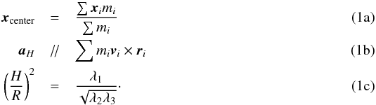 The quantities x and m with subscript i indicate the position and mass of each cell inside the ellipsoid; aH is the vector representing the direction of the minor axis. The eigenvalues of the moment of inertia are λ1,2,3 in increasing order. This procedure defines a series of self-consistent ellipsoids contained within each other. The disordered nature of the flow causes the ellipsoids to be not necessarily similar nor aligned.
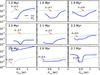 |
Fig. 4 Examples of the piecewise fit at nine time steps for the run with tff/tvct = 0.9. The normalized residual is plotted as function of cluster characteristic radius |
3.1.2. Step 2: The fitting procedure
A cloud forming a central cluster features a collapsing envelope and a quasi-stationary core with minor infalling motion. To distinguish between the two, we define a quantity 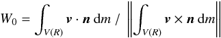 (2)for the series of ellipsoids of different size to observe the change in the collapsing motion, where v is the velocity and n the unit vector pointing from the ellipsoid center to the cell position. While the envelope is expected to be globally infalling, the gaseous protocluster itself should be relatively stationary with more prominent rotation. The quantity W0 should therefore follow different radial dependence inside and outside the protocluster. We show with simple arguments that its numerator F0 = ∫v·n dm follows different radial dependences inside and outside the gaseous protocluster. By making analogy to the collapsing phase of the Larson-Penston solution of a sphere (Larson 1969; Penston 1969), where the mass flux is conserved for all radii (ρ ∝ r-2 and vinf ∝ const.) in a stationary state, we conclude that F0 should be roughly proportional to R in the envelope,
 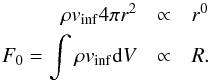 (3)As for the region inside the gaseous protocluster, the assumption of uniform density implies that the density increasing rate is also uniform. We deduce that F0 ∝ R4, i.e.,
 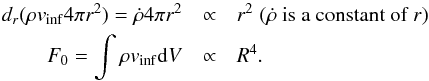 (4)Though these are not exact derivations for a configuration with rotation, a difference in radial dependence is clear when a quasi-stationary core exists. We therefore propose a simple piecewise power-law description that differentiates the flow properties inside and outside the gaseous protocluster. As shown in Fig. 4, the infall moment exhibits a change in slope in log scale. Inside the cluster, the gas is no longer necessarily collapsing and W0 can even change signs. A piecewise fit is performed and the residual calculated to define the semimajor axis R∗ of the gaseous protocluster. This expression is written as
 ![% subequation 1553 0 \begin{align} W_{0,\mathrm{fit}}(R_\mathrm{avg}, r_\ast) &= \left\{ \begin{array}{lcl} a_{\rm c} R_\mathrm{avg}^{b_{\rm c}} & \mbox{for} & R_\mathrm{avg}<r_\ast \\ a_{\rm e} R_\mathrm{avg}^{b_{\rm e}} & \mbox{for} & R_\mathrm{avg}>r_\ast \end{array} \right. \\ res(r_\ast) &={1\over n_R} \sum_R \left[ \frac{W_{0,\mathrm{fit}}(R_\mathrm{avg}, r_\ast) - W_0(R)}{W_0(R)} \right]^2 \\ R_\ast &= \arg \min{res(r_\ast).} \end{align}](/articles/aa/full_html/2016/07/aa27981-15/aa27981-15-eq62.png) The average radius of the ellipsoid
The average radius of the ellipsoid  is used to perform the power-law fit since it is the most proper value to represent the ellipsoid. The choice of this quantity is discussed in Appendix A. The inner part of the fitted function is put to zero when there are fluctuations around zero, and the negative points are omitted when fitting the outer part. The size of the gaseous protocluster is defined as the radius at which the minimal local minimum occurs. This normalized residual of the best fit is usually smaller than 10-3, and its square root implies an error of a few percentage of the fit. The fit residual is large when there are changes in sign of W0 as a result of our definition of the functions, but the radius is on the contrary very well defined in such cases. A local minimum of the fit residual cannot always be found. This might be because the gas is highly turbulent and that there is a fluctuating shock zone between the envelope and gaseous protocluster, which deteriorates the fit if it is included in either of the two domains. Nonetheless, when it exists, it marks well the transition between the two regimes. Moreover as described below, the results obtained are entirely reasonable with the gaseous protocluster radius inferred indicating the dense central region that we see generally well.
3.1.3. Results
The inferred evolution of the size and mass of the cluster are presented in Fig. 5. Despite its turbulent nature, the size of the gaseous protocluster stays relatively constant while mass is accreted. The more turbulent the initial cloud is, the larger the protocluster is. The mass evolution is plotted with the gas mass and total mass (sinks inside the ellipsoid included). The gas mass stays roughly constant while the total mass increases, implying that most of the mass accreted onto the cluster ends up in the sinks. As expected, the radius drops with αvir because of the weaker rotational and turbulent support. This is reproduced by the analytical model developed in Paper II. It is important to note that these simulations are performed without feedback from the sink particles as a result of core or star formation. With feedback considered, the sink formation and accretion could be substantially delayed and/or reduced.
3.2. The embedded sink cluster
3.2.1. A simple method
As recalled previously, in the simulations, sink particles are formed to follow regions of concentrated mass. Those regions are the places where stars are likely to form, therefore the sink particle distribution is representative of the stellar cluster and the cluster size can be inferred from the distribution of the sink particles. This is carried out by computing the three eigenvalues of the rotational inertia matrix of sink particles with respect to their center of gravity. As the eigenvalues represent the widths in three orthogonal directions, they reveal not only the size but also the shape of the sink particle cluster. The rotational inertia matrix is 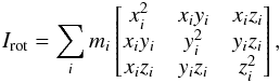 (6)where i is the index of sink particles. Its three eigenvalues λ1,λ2,λ3 give the cluster size in three orthogonal directions as follows:
 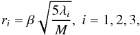 (7)where M is the total mass of sinks. The factor 5 comes from the assumption that the sink mass is uniformly distributed in space, and a correctional factor β ≥ 1 accounts for the fact that the mass distribution might not be uniform but rather centrally concentrated.
From a first calculation (see dashed lines in Fig. 6), it is clear that the sink particles are very extendedly distributed, and that the concentration in certain directions gives a relative large eigenvalue compared to the other two. However, as we saw before, some sink particles are forming in filaments feeding the cluster (see Fig. 2), which is consistent with previous calculations and, therefore, are not located inside the cluster. Furthermore, there are also sinks that are ejected from the cluster through N-body interactions. These sinks, however, should not be taken into account when studying the cluster itself. We therefore refine the calculation by omitting the sink particles that have larger distances than the largest semiaxis from the first calculation and repeating the same procedure. This operation is not always converging, therefore, we search for convergence by increasing β starting from unity. When β is large enough, convergence is reached in just a couple of iterations. We employ the smallest β value that yields convergence, which goes up to about 1.5 at its highest (implying that β is always between 1 and 1.5). This yields a cluster which is more spherical and stays roughly constant in size as the total sink mass increases.
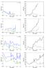 |
Fig. 5 Time evolution of the semiaxes R and H of the ellipsoidal gas cluster in the left column. In the right column, the cluster mass is shown as function of time. The two curves represent the gas mass (dashed) and that plus the sink mass (solid) inside the ellipsoidal region defined with gas kinematics. From top to bottom are runs A, B, C, and D with increasing levels of turbulence. The protocluster size increases with turbulence level. Most of the mass is accreted onto the sinks while the cluster mass increases in time, therefore the gas mass stays roughly constant. |
The evolution of the sink cluster radius and mass are plotted in Fig. 6. The total mass of all sinks is plotted in dotted curves while that of those inside the cluster is plotted with dashed curves. The total mass including the gas is also plotted in solid curves. At early times right after the formation of the first sinks, the inferred cluster size fluctuates and could reach very high values. These are possibly the cases where there exist very few sinks, which form in the surrounding filaments, and therefore the algorithm fails. The selection of clustered sinks is not always robust, and the inferred size shows spiky fluctuations despite the generally stable trend it exhibits. However, the significantly reduced size and relatively mild decrease in mass suggest that the distant sinks,which make up only a small fraction of the mass, are effectively rejected.
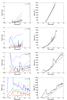 |
Fig. 6 Time evolution of the three semiaxes of the cluster determined with sink particles in the left column. The dashed curves and solid curves represent the values calculated with all sinks and the reduced values with distant sinks omitted, respectively. The sink mass (dashed) and total mass (solid) inside cluster region defined with sink distributions are plotted against time in the right column. The dotted line represents the sink mass before sink removal. Removing the sink particles far away from the center drastically reduces the size while only mildly decreasing the total mass. From top to bottom are runs A, B, C, and D with increasing levels of turbulence. |
3.2.2. Minimal spanning tree
It is instructive to confront these results with those obtained using another method. The minimal spanning tree method (MST; Gower & Ross 1969; Cartwright & Whitworth 2004) is also applied to examine the selection of sinks belonging to the cluster. The MST is obtained by linking all the points in a cluster with a tree-like structure, while minimizing the sum of the length of the links without forming loops. One way to find the MST is to start with the two closest points, and one shortest branch is added each time to link one more point to whichever point in the group. A critical value Lcrit, the longest branch length allowed inside a cluster, is used to define the members of a cluster. The method used by Gutermuth et al. (2009) to determine Lcrit with the cumulative distribution function of the branch length does not work well with our data set, since there are many closely located sinks and this makes the steep-slope segment extremely steep, thus, rejecting more than half of the sinks. If we plot the radius calculated for the selected set of sinks as a function of Lcrit, it could be seen that with Lcrit increasing, there are abrupt jumps in the cluster size. These events indicate that a previously considered distant sink or group of sinks is included in the cluster and this distance is comparable with respect to the original cluster size. This picture is consistent with the fractal nature of the cluster structure.
Some examples of the MST radius-Lcrit plot are shown in Fig. 7, and several plateaux appear, which all indicate possible cluster radius. This is compatible with the fluctuations of radius defined with the previous method. We attempted to select the plateau of which the rotational axis aligns best with the minor axis, while the optimal match usually occurs for a very small group of sinks. Therefore, an automatic determination of cluster member selection is not straightforward. Nonetheless, most of the time we see one of the plateaux corresponding very well to the radius calculated with the relatively simple sink selection we proposed. Consequently, we conclude that using a simple selection criteria, such as the one we presented to characterize the cluster, leads to reasonable results.
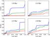 |
Fig. 7 Three semiaxes calculated from the rotational inertia matrix with the assumption of uniform mass distribution, plotted against Lcrit, which is the maximal allowed distance linking a member to the cluster. Examples are shown for four time steps of run B. |
3.2.3. Other methods
We also tried inferring the sink cluster radius according to the rms distance to the center weighted by local density proposed by Casertano & Hut (1985). The local density (number or mass) is calculated for each sink considering the ith nearest neighbor, and the cluster center is also determined by the density-weighted position. The inferred radius is typically less than 10-2 pc and is very dependent on the number of neighbors used. This comes probably from the same problem, which we mentioned in the previous paragraph, that the sink particles are very close to each other at the central part of the cluster and therefore create extremely high local densities. The local density could have a contrast of several orders of magnitude for sinks at different locations, and the central sinks are thus heavily weighted, yielding a small radius. In a slightly different approach, Portegies Zwart et al. (2010) suggested using the squared density as the weight. In our case, this only make the problem more serious.
There is another method that uses the local density. A neighborhood radius is first determined from the distribution of the sink distances. A sink is included in the cluster if the number of sinks in its neighborhood exceed the threshold, which comes from the level of significance required for detection. The cluster size is then calculated with the minimal convex hull that contains all the cluster members (Joncour, in prep.). This method detects the departure from a random distribution and finds the overdense region. Again, as a result of the characteristics of our sink distribution, the treatment of multiple systems may also play an important role (internal communication) and special care needs to be taken when selecting the parameters. With properly selected parameters, the sink cluster radius is similar to what we found with the inertia momentum.
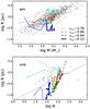 |
Fig. 8 Upper panel: gaseous protocluster mass-size relation defined with gas kinematics overplotted with measurements of star-forming clumps summarized by Fall et al. (2010, light gray dots) and Urquhart et al. (2014, dark gray dots). The total mass of the cluster is used (gas plus sinks). Lower panel: sink cluster number-size relation overplotted with embedded cluster concluded by Adams et al. (2006, dark gray dots) and Gutermuth et al. (2009, light gray dots). The gray line indicates the number-size relation R (pc) ∝ (N/ 300)1/2 by Adams et al. (2006). Simulations with four different levels of turbulent support are plotted. The blue solid, green dashed, red dot-dashed, and cyan dotted curves have virial parameters αvir = 0.12, 0.64, 0.96, 1.78, respectively. The curves represent the time sequence. As the protoclusters accrete, they gain in mass and move from left to right in the figure. Time steps before 2 Myr are plotted with thinner lines. |
The above described methods are set out from observational points of view with the goal of defining a local concentration and its extension. As we discussed, the definition of a cluster is not trivial and depends to a large degree on the parameters used. Therefore there is always some uncertainties in its determination. Our simulations do not have sufficient resolution to resolve individual stars, therefore methods using local properties tend to work less well. The cluster inferred using the moment of inertia captures the mass distribution at the cluster scale and is more pertinent at least for consistent comparison among simulations.
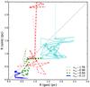 |
Fig. 9 Radius of sink clusters plotted against radius of gas protoclusters for four runs. The relations are plotted with thinner lines for time before 2 Myr and with thicker lines after 3 Myr. The color coding is the same as that in Fig. 8. The gas and sink cluster sizes show good correlation in general, while the sink cluster size is slightly smaller than that of the gas cluster. |
3.3. The cluster mass-size relation
The mass-size relation is one of the important characteristics of protoclusters that can be compared with observations. In Fig. 8, the mass-size relations of gaseous protoclusters defined with gas kinematics are overplotted with observations of star-forming clumps (Fall et al. 2010; Urquhart et al. 2014), and the number-size relations of clusters obtained from sink distributions are overplotted with embedded cluster observations (Adams et al. 2006; Gutermuth et al. 2009). Early time steps (before 2 Myr) are plotted with thinner lines. As the gaseous protocluster accretes mass, it arrives on the observed sequence. The larger the turbulence in the parent cloud, the more expanded the protocluster since the mass feeding the protocluster has higher kinetic energy and the rotation is also more important. For the sake of comparison with observations, we also show the relation obtained by Adams et al. (2006)R (pc) ∝ (N/ 300)1/2. The sink clusters come close to this sequence after sufficient evolution. At a later stage, they form fewer new sinks and start increasing in radius. Further discussion is needed, however, as our sinks are massive and do not represent individual stars. The number-size (or mass-size) relation inferred with sink particles is thus biased and not exactly representative of the embedded cluster itself. The absence of feedback in our simulations translates into over formation of sink particles and their over accretion (overestimation of star numbers and mass), and these sinks represent prestellar cores that might form stars inside (underestimation of star numbers) with some efficiency (overestimation of star mass). The overall effect is possibly a shift of the number-size relation in the lower panel of Fig. 8 toward the right, where the upper limit 20 is the ratio between averaged sink mass (10 M⊙) and averaged stellar mass (0.5 M⊙). On the other hand, the cluster is a hierarchical structure. The size is very dependent on the membership selection and there could easily be a factor 2 difference in radius (see Figs. 6, 7) as a consequence of different sensitivity and criteria used, which would lead to a factor 10 in density uncertainties. The expansion of cluster after gas removal by stellar feedback is not included in our simulations, giving another possible underestimation of the cluster radius. Considering all these uncertainties, we cannot readily reproduce the number-size relationship for embedded clusters, but they should at least not be too far away from the observed sequence. Observationally speaking, Pfalzner et al. (2016) plotted the number-size relation for different star-forming regions and found that, even though this relation follows the same trend inside different regions, its absolute value in number can vary by a factor 20 (their Fig. 3). The cluster definition and distance of the object could play important roles. On the other hand, we see that the sink cluster radius does not change very much with time, at least telling us that at the early stage of stellar cluster formation, these clusters should still somewhat be correlated to and regulated by their natal gas. We stress that according to our analysis, the link between the gaseous protocluster radius and that of the embedded cluster is not a trivial matter. Therefore, the 20% efficiency that is usually inferred should be regarded with great care.
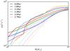 |
Fig. 10 The specific angular momentum plotted against mass contained inside ellipsoids of varying radius at a series of time steps of run B. Solid curves represent the specific angular momentum of gas. Dashed curves represent the averaged value considering gas and sinks at the same time. The specific angular momentum of gas is more or less conserved during the collapse, which justifies our simplification, while the sink particles exhibit a loss in angular momentum. |
We compare the cluster size inferred with gas and sinks in Fig. 9. The sink clusters generally are smaller in size than the gas clusters. This implies that the stars are possibly formed in the inner region of the gaseous protocluster. The relations are plotted with a line thickness that increases with time. We can see in both the green and red curves that at early time the sink cluster radius is large probably due to the bad definition of a cluster with very few sinks. Once the cluster becomes steadily established (after 2 Myr), they show a radius that is smaller than the gaseous protocluster size. At an even later time (after 3 Myr with the thickest lines), the sink cluster radius shows a growth with respect to the gas radius. This might be a sign of the dynamical decoupling and expansion of the stellar cluster. Evidence of the sink-gas decoupling is indeed shown in Fig. 10, where we plot specific angular momentum of gas (solid curves) and gas plus sinks (dashed curves) in concentric ellipsoids against mass at several time steps. For a fixed mass, the region concerned is shrinking in time under the collapse. The solid curves are relatively close to one another, which means that in one collapsing mass entity, the averaged gas specific angular momentum does not vary significantly in time. Moreover, we see that while the total angular momentum (dashed curves) is conserved at high mass (M ≳ 5 × 10³ M⊙), it decreases at lower mass, indicating that the angular momentum is transported away. We conclude that while the gas more or less conserves its angular momentum during the collapse, the momentum of the sinks is lost gradually. Longmore et al. (2014) concluded that the gas-star coevolution cannot continue over a dynamical time, on the one hand, because the gas is dissipative while stars are ballistic and, on the other hand, because stars form from gravitational collapse of gas and create a local, gas-free environment for themselves. Also mentioned by Bate et al. (2003), the gas-star interaction plays a very important role in regulating star formation. Parker & Dale (2015) perform a Q-parameter analysis (Cartwright & Whitworth 2004) of gas and stars in simulations and suggest that their spatial distributions are not trivially linked. This sheds light on the importance of correctly following both gas and particle dynamics in simulations and the necessity of pertinent theories of early stellar cluster formation.
To conclude, our simulations successfully reproduce the mass-size regions that we define as gaseous protoclusters provided the virial parameter αvir is large enough. When the cloud is too weakly supported (small αvir), the gaseous protocluster is strongly accreting and has a small radius and this should probably not be compared to the observations. For other runs of clouds with αvir close to unity, a good agreement of the mass-size relation between observations and simulations is reached. As gaseous protoclusters accrete mass, they arrive on the observed sequence, which very likely implies a stationary and quasi-equilibrium state.
Although we have performed simulations of 104 M⊙ clouds, giving gaseous protoclusters of a few thousand solar masses, the gas is almost isothermal at the cloud and protocluster scale and the results could then be rescaled to the observed mass range. The simulations are parametrized by the following two nondimensional numbers:  (8)If we rescale the molecular cloud in the simulation to different mass, size, and temperature such that
  (9)where γ = 1or0.7 is the exponent in the Larson relation ρ ∝ R− γ (Larson 1981; Falgarone et al. 2004, 2009; Hennebelle & Falgarone 2012; Lombardi et al. 2010) and A is a scaling factor. With this rescaling, αvir and ℳ stay unchanged, and the new cloud also follows the Larson relation. The gaseous protocluster inside the cloud is therefore rescaled, following
  . This implies that given parent clouds that follow Larson relations, the gaseous protoclusters formed therein follow relation reported by Fall et al. (2010) and Urquhart et al. (2014). Indeed in Paper II, an analytical model is developed to account for the mass-size relation of gaseous protoclusters of any mass. Given the turbulence level and mass of the parent cloud, the model predicts the mass, size, aspect ratio, and velocity dispersion of the gaseous protocluster. As long as the condition that stellar feedback is not very important stays valid, our simulations and analytical model match the observations of low-mass, gaseous protoclusters.
Stars form from the gas reservoir in the gaseous protocluster. Properties possessed by the gas should be to some extent passed down to the stars. Once formed, the stars, however, start to dynamically depart from the natal gas. Links between the protocluster gas and the stellar cluster should be carefully made to yield comprehensive comparisons and shed light on their different dynamical properties. This is seen in the mass-size relations derived from observations of stars in the embedded cluster (Adams et al. 2006) and gas of star-forming clumps (Fall et al. 2010; Urquhart et al. 2014). Though showing the same trend, these relations exhibit a shift in absolute value (Pfalzner et al. 2016). If we assume a 0.5 M⊙ averaged mass for the stars inside the clusters, a star formation efficiency of less than 10% is required to reconcile the two relations given that the cluster size does not evolve. Alternatively, this could also be explained by an expansion after the cluster formation. We inferred the cluster size for gas and sinks, which enables a comparison between the two and allows us to compare the cluster size with observations as well.
4. Internal properties of the protocluster
Now that we defined the cluster in the simulations, we can calculate its mass, size, angular momentum, velocity dispersion, and various quantities. In this section, we perform some analyses of the protocluster properties since these analyses are important for understanding in which conditions stars form.
4.1. Energies equilibrium
Once the protocluster is identified, we proceed to calculate the energies in different forms inside this region and examine the balance. Since we are discussing the gas-dominated early phase of cluster formation, we use the protoclusters previously defined with gas kinematics, which indeed show good correspondence with observations. The specific kinetic, gravitational, thermal, and magnetic energies are plotted at several time steps in the top panel of Fig. 11. The gravitational energy is negative and is plotted in absolute value. Here we only show the run with tff/tvct = 0.9 since all the runs exhibit similar trends. Results of other runs are shown in Appendix B.
For the gas component (green), the thermal and magnetic energies are a few percent of the gravitational energy, which is consistent with that initialized in the parent cloud and, therefore, do not contribute much to supporting against self-gravity at the cluster scale. The specific thermal energy stays roughly constant and decreases mildly, indicating a slight temperature decrease due to density increase. The specific magnetic energy increases slightly as a result of magnetic flux concentration. On the other hand, the kinetic energy, which has contributions from turbulence and rotation, acts largely to support against gravitational contraction.
The cluster satisfies 2Ekin,g + Egrav,g ≈ 0, indicating the gas component is in virial equilibrium while the cluster is accreting mass. The particle component (yellow), on the other hand, begins to have higher specific kinetic and gravitational energies a short while after the sinks start forming. This implies that the sink particles are more centrally concentrated than the gas and lie in a deeper potential well, which is consistent with our previous finding that the radius determined with sinks is smaller (Fig. 9). This is compatible with the discovery by Bate et al. (2003) that the stars have velocity dispersion that is three times higher than that of the gas. It is remarkable that the sinks are bound almost at virial and satisfy the relation 2Ekin,s + Egrav,s ≈ 0, indicating that the cluster energy properties are largely inherited from its natal gas and are determined at the early formation stage. Walker et al. (2016) suggested that clusters very likely form in a conveyor-belt mode, in which the core of the star-forming cloud accumulates mass at the same time as stars form. This is perfectly in coherence with our simulation results that stars form in the dense, gaseous protocluster, of which the mass and energy is sustained by accretion.
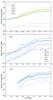 |
Fig. 11 Top: different forms of specific energy of the cluster defined with gas kinematics plotted against time. The gas component is plotted in green and the sinks are plotted in yellow. The solid, dashed, dotted, and dash-dotted lines represent kinetic, gravitational, thermal, and magnetic energies respectively. The gravitational energy is plotted in absolute value. Middle and bottom: kinetic (blue) and gravitational energy (cyan) decomposition of the gas component (middle panel) and the sink component (bottom panel) of the protocluster plotted in specific values. Total energy, energy along z-axis, rotational energy, and energy perpendicular to z-axis are plotted with solid lines, dashed lines, dash-dotted lines, and dotted lines respectively. |
4.2. Rotation and turbulence anisotropy
The rotation makes up an important part of the kinetic energy of the protocluster and a flattened form is thus a natural consequence. We estimate the rotational energy of the protocluster and separate it from its turbulent counterpart. This allows us to compare the proportions of rotational and turbulent energies and also examine whether turbulence is isotropic. The rotational energy is estimated as  , where J is the total angular momentum vector of the cluster, and I is its rotational inertia matrix. This allows us to eliminate turbulence by summing up various motions. Uncertainties remain, in particular, since we do not take into account the differential rotation, this is probably an underestimation. The one-dimensional turbulent energy along the rotational axis of the cluster Ekin,z is also calculated. The turbulent energy perpendicular to the rotational axis could be thus estimated as Ekin,r = Ekin − Ekin,rot − Ekin,z. We display the energies for the run with tff/tvct = 0.9. Other results are shown in Appendix B. In the middle panel of Fig. 11, we plot the total kinetic energy, rotational energy, turbulence parallel and perpendicular to the rotational axis, respectively, for the gas component in blue. The proportion of rotational energy becomes more and more important as the gaseous protocluster accretes, while that of Ekin,z is slightly decreasing. The rotational energy grows to become comparable to the turbulent energy in the same plane and makes up nearly a third of the total kinetic energy. The turbulence shows anisotropy since Ekin,r/Ekin,z> 2, although there remain uncertainties in the estimation of the rotation. The rotation flattens the protocluster and this anisotropy in geometry thus makes the kinetic energy distribution anisotropic in turn.
We also plot in cyan the gravitational energy of the cluster (Egrav). The gravitational energy is calculated by integrating the dot product of the gravity and the position vector with respect to cluster center over the cluster volume (as is carrried out in the virial theorem). With this definition, we can separate the gravitational energy into two contributions by calculating respectively with the gravitational acceleration parallel (Egrav,z) and perpendicular (Egrav,r) to the cluster minor axis (see Paper II for definitions). This points out the fact that not only the protocluster is generally in virial equilibrium, but it also satisfies a modified virial theorem that accounts for the two dimensions, i.e., 2Ekin,z + Egrav,z ≈ 0 and 2Ekin,r + 2Ekin,rot + Egrav,r ≈ 0. This motivates the decomposition of the virial theorem into two dimensions in the analytical model in Paper II. The bottom panel of Fig. 11 shows the same plot as that in the middle for the sink component of the protocluster. The sink particles show similar trends to the gas in general. A very different behavior is that the rotational energy calculated for the whole system is not increasing like that of the gas. Moreover, Ekin,rot ≪ Ekin, indicating that the stars are giving angular momentum to the gas and there is less a general rotation.
4.3. Density PDF
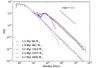 |
Fig. 12 In solid curves for the gaseous protocluster and in dashed curves for the parent cloud, the PDF at several time steps for run B with tff/tvct = 0.9. The total mass of the protocluster is indicated in the legend. The normalization is performed such that the integral is equal to one. The distribution is close to lognormal at the beginning as a result of turbulence interaction. The gravity soon dominates and creates a prominent power-law tail. The slope −2.2 is the average of the cluster PDF slopes evaluated at the same density range as the black line except for the first time step. |
The star formation is a result of collapse induced by local overdensity, therefore, essential information is imprinted in the density probability density function (PDF) of the star-forming environment, which is in turn a result of interaction between turbulence and gravity. The density PDF is important for theoretical prediction of the IMF such as that of Padoan & Nordlund (2002), Hennebelle & Chabrier (2008, 2009), and Hopkins (2012). We plot the density PDFs of the gaseous protoclusters identified in the previous section and that of the parent cloud, and show that there are indeed fundamental differences.
In Fig. 12, the volume-weighted PDF of the gaseous protocluster and that of the parent cloud are plotted at several time steps. At the beginning of the simulation, the PDF is very close to a log-normal distribution, which is a natural consequence of the turbulence, while the gravity soon dominates at later times. The gaseous protocluster shows the same power-law, high-mass tail as the parent cloud with a slope −2.2, which is a signature of local gravitational collapse. This is a common feature of star-forming region as first mentioned observationally by Kainulainen et al. (2009). The major difference lies in that the gaseous protocluster region is denser than the original cloud environment with a density peak around 104 H cc-1. The power-law exponent is slightly steeper than that expected from the self-similar Larson-Penston collapse (−1.5) or the expansion wave collapse solution (−2; Larson 1969; Penston 1969; Shu 1977; Kritsuk et al. 2011). The density PDF of the cloud stays almost unchanged while a gaseous protocluster develops within. This emphasizes the fact that when the stars form, their environment is already not the same as the cloud in which they reside. Inside the gaseous protocluster, the gas properties are modified by the interaction of gravity and turbulence. The gaseous protocluster stage should therefore be taken into account when linking the molecular cloud to the stellar cluster.
4.4. Discussion
It is still an unanswered question whether the universality of the IMF is a result of similar star formation processes in various kinds of environment, or a fruit of coincidence by different factors canceling out. Understanding the underlying mechanisms of star formation is therefore essential. One key question to answer is whether star formation is dominated by its environment, i.e., the initial gas reservoir available, or by the local gas flow properties.
Stellar clusters are ideal locations to provide statistics on star formation and to study the interaction of stars and their environment. Stars form inside the gaseous protocluster where the gas is reprocessed during the gravoturbulent collapse of the parent cloud. Compared to a molecular cloud, which more or less follows the Larson relations, the gaseous protocluster environment is indeed different as can be seen with the mass-size relation. They are ten times more massive than the clouds at the same size. The density PDFs also exhibit significant differences, which have fundamental influences on the overdensity seeding of prestellar cores. Finding a mapping from the parent cloud to the gaseous protocluster would provide an intermediate link between the initial diffuse cloud gas and the dense prestellar cores and, therefore, to some extent decouple the core formation and initial cloud conditions if the gaseous protocluster properties are more or less general, regardless of the parent cloud.
Given our results, we could thus reasonably propose the scenario that the gaseous protocluster has its turbulence primarily driven by the accretion, as is a universal process described by Klessen & Hennebelle (2010) and Goldbaum et al. (2011); this turbulence acts as a support against self-gravity, while at the same time, the rotation is important since at this scale the loss of angular momentum by its outward transport remains limited. It is therefore clear that a primary gas-dominated protocluster stage can be defined before cluster formation. In the companion paper (Paper II) we introduce an analytical model that describes an accreting ellipsoidal system in virial equilibrium and demonstrates that the gaseous protoclusters lie on a sequence of global equilibrium as a result of the interplay between turbulence and gravity. We derive a mapping from the cloud parameters to the gaseous protocluster properties.
5. Conclusions
Star formation is a hierarchical process that incorporates multiple spatial and temporal scales, where the interaction of turbulence and gravity plays an essential role. In this paper, we focus on the very beginning stage of stellar cluster formation. We propose that a primary structure, the gaseous protocluster, is first created out of the collapsing molecular cloud and it reaches a state of global virial equilibrium as a consequence of the gravoturbulent interaction. The gaseous protocluster subsequently evolves into the stellar cluster, which inherits its equilibrium properties from the gas.
A series of collapsing molecular clouds are simulated to form gaseous protoclusters, and a sink particle algorithm is used to follow prestellar cores. The gaseous protocluster is clearly identifiable after about 2 Myr, while its boundary is very irregular. The gas kinematics and sink particle distributions are used to determine the protocluster region, an ellipsoid flattened by its prominent rotation. We define a measure of infall motion against rotation of the gas as an integrated property, and infer the size of the gaseous protocluster by distinguishing between the collapsing envelope and the quasi-stationary core. The sink particle distribution is used to calculate the rotational inertia, and, in turn, yields the size and shape of the cluster. The protoclusters inferred with the aforementioned methods are compared to the observed star-forming clumps and embedded clusters, respectively. Both the gas and sink clusters show stationary behavior in size and are coherent with observations. We stress that although the stellar cluster radius and the gaseous protocluster radius are correlated, their exact values are sensitive to the definition adopted. Therefore, this implies that any interpretation in terms of gas removal or efficiency should be taken with care.
From the energy analysis, the protocluster is in virial equilibrium such that the rotation and turbulence support against self-gravity. As turbulence is driven by the accretion from the collapsing molecular cloud, a new balance is established in this emerging entity. This is obviously prescribed by the properties of the parent cloud and the nature of its collapse. The initial turbulence level in the parent cloud is also imprinted in that of the gaseous protocluster and, consequently, determines its size. We conclude that the gaseous protocluster is indeed an important intermediate step of stellar cluster formation from molecular clouds, and that star formation should be studied in this context. This work does not take stellar feedback into account . To fully describe the protocluster at later times, a more complete model considering the gas-sink interaction is necessary.
Acknowledgments
This work was granted access to HPC resources of CINES under the allocation x2014047023 made by GENCI (Grand Equipement National de Calcul Intensif). This research has received funding from the European Research Council under the European Community’s Seventh Framework Programme (FP7/2007-2013 Grant Agreement No. 306483). The authors thank the anonymous referee for the careful reading and useful suggestions.
References
- Adams, F. C., Proszkow, E. M., Fatuzzo, M., & Myers, P. C. 2006, ApJ, 641, 504 [NASA ADS] [CrossRef] [Google Scholar]
- Audit, E., & Hennebelle, P. 2005, A&A, 433, 1 [NASA ADS] [CrossRef] [EDP Sciences] [Google Scholar]
- Ballesteros-Paredes, J., Hartmann, L. W., Pérez-Goytia, N., & Kuznetsova, A. 2015, MNRAS, 452, 566 [NASA ADS] [CrossRef] [Google Scholar]
- Bate, M. R. 2009, MNRAS, 392, 1363 [NASA ADS] [CrossRef] [Google Scholar]
- Bate, M. R. 2012, MNRAS, 419, 3115 [NASA ADS] [CrossRef] [Google Scholar]
- Bate, M. R., Bonnell, I. A., & Bromm, V. 2003, MNRAS, 339, 577 [NASA ADS] [CrossRef] [Google Scholar]
- Bleuler, A., & Teyssier, R. 2014, MNRAS, 445, 4015 [NASA ADS] [CrossRef] [Google Scholar]
- Bonnell, I. A., Bate, M. R., & Vine, S. G. 2003, MNRAS, 343, 413 [NASA ADS] [CrossRef] [Google Scholar]
- Bonnell, I. A., Clark, P., & Bate, M. R. 2008, MNRAS, 389, 1556 [NASA ADS] [CrossRef] [Google Scholar]
- Carpenter, J. M. 2000, AJ, 120, 3139 [NASA ADS] [CrossRef] [Google Scholar]
- Cartwright, A., & Whitworth, A. P. 2004, MNRAS, 348, 589 [NASA ADS] [CrossRef] [Google Scholar]
- Casertano, S., & Hut, P. 1985, ApJ, 298, 80 [Google Scholar]
- Commerçon, B., Hennebelle, P., & Henning, T. 2011, ApJ, 742, L9 [NASA ADS] [CrossRef] [Google Scholar]
- Dale, J. E., Ercolano, B., & Bonnell, I. A. 2013a, MNRAS, 431, 1062 [NASA ADS] [CrossRef] [Google Scholar]
- Dale, J. E., Ercolano, B., & Bonnell, I. A. 2013b, MNRAS, 430, 234 [NASA ADS] [CrossRef] [MathSciNet] [Google Scholar]
- Dale, J. E., Ngoumou, J., Ercolano, B., & Bonnell, I. A. 2013c, MNRAS, 436, 3430 [NASA ADS] [CrossRef] [Google Scholar]
- Dale, J. E., Ercolano, B., & Bonnell, I. A. 2015, MNRAS, 451, 987 [NASA ADS] [CrossRef] [Google Scholar]
- Davies, B., Bastian, N., Gieles, M., et al. 2011, MNRAS, 411, 1386 [NASA ADS] [CrossRef] [Google Scholar]
- Falgarone, E., Hily-Blant, P., & Levrier, F. 2004, Ap&SS, 292, 89 [NASA ADS] [CrossRef] [Google Scholar]
- Falgarone, E., Pety, J., & Hily-Blant, P. 2009, A&A, 507, 355 [NASA ADS] [CrossRef] [EDP Sciences] [Google Scholar]
- Fall, S. M., Krumholz, M. R., & Matzner, C. D. 2010, ApJ, 710, L142 [NASA ADS] [CrossRef] [Google Scholar]
- Faúndez, S., Bronfman, L., Garay, G., et al. 2004, A&A, 426, 97 [NASA ADS] [CrossRef] [EDP Sciences] [Google Scholar]
- Federrath, C. 2015, MNRAS, 450, 4035 [NASA ADS] [CrossRef] [Google Scholar]
- Federrath, C., Schrön, M., Banerjee, R., & Klessen, R. S. 2014, ApJ, 790, 128 [NASA ADS] [CrossRef] [Google Scholar]
- Fontani, F., Beltrán, M. T., Brand, J., et al. 2005, A&A, 432, 921 [NASA ADS] [CrossRef] [EDP Sciences] [Google Scholar]
- Fromang, S., Hennebelle, P., & Teyssier, R. 2006, A&A, 457, 371 [NASA ADS] [CrossRef] [EDP Sciences] [Google Scholar]
- Fujii, M. S., & Portegies Zwart, S. 2015, MNRAS, 449, 726 [NASA ADS] [CrossRef] [Google Scholar]
- Geen, S., Hennebelle, P., Tremblin, P., & Rosdahl, J. 2015, MNRAS, 454, 4484 [NASA ADS] [CrossRef] [Google Scholar]
- Girichidis, P., Federrath, C., Banerjee, R., & Klessen, R. S. 2011, MNRAS, 413, 2741 [NASA ADS] [CrossRef] [Google Scholar]
- Girichidis, P., Federrath, C., Banerjee, R., & Klessen, R. S. 2012, MNRAS, 420, 613 [NASA ADS] [CrossRef] [Google Scholar]
- Goldbaum, N. J., Krumholz, M. R., Matzner, C. D., & McKee, C. F. 2011, ApJ, 738, 101 [NASA ADS] [CrossRef] [Google Scholar]
- Gower, J. C., & Ross, G. J. S. 1969, J. Roy. Statist. Soc. Ser. C, 18, 54 [Google Scholar]
- Gutermuth, R. A., Megeath, S. T., Myers, P. C., et al. 2009, ApJS, 184, 18 [NASA ADS] [CrossRef] [Google Scholar]
- Hénault-Brunet, V., Gieles, M., Evans, C. J., et al. 2012, A&A, 545, L1 [NASA ADS] [CrossRef] [EDP Sciences] [Google Scholar]
- Hennebelle, P. 2012, A&A, 545, A147 [NASA ADS] [CrossRef] [EDP Sciences] [Google Scholar]
- Hennebelle, P., & Chabrier, G. 2008, ApJ, 684, 395 [NASA ADS] [CrossRef] [Google Scholar]
- Hennebelle, P., & Chabrier, G. 2009, ApJ, 702, 1428 [NASA ADS] [CrossRef] [Google Scholar]
- Hennebelle, P., & Falgarone, E. 2012, A&ARv, 20, 55 [NASA ADS] [CrossRef] [Google Scholar]
- Hopkins, P. F. 2012, MNRAS, 423, 2037 [NASA ADS] [CrossRef] [Google Scholar]
- Iffrig, O., & Hennebelle, P. 2015, A&A, 576, A95 [NASA ADS] [CrossRef] [EDP Sciences] [Google Scholar]
- Kainulainen, J., Beuther, H., Henning, T., & Plume, R. 2009, A&A, 508, L35 [NASA ADS] [CrossRef] [EDP Sciences] [Google Scholar]
- Klessen, R. S., & Burkert, A. 2000, ApJS, 128, 287 [NASA ADS] [CrossRef] [Google Scholar]
- Klessen, R. S., & Hennebelle, P. 2010, A&A, 520, A17 [NASA ADS] [CrossRef] [EDP Sciences] [Google Scholar]
- Klessen, R. S., Burkert, A., & Bate, M. R. 1998, ApJ, 501, L205 [NASA ADS] [CrossRef] [Google Scholar]
- Kritsuk, A. G., Norman, M. L., & Wagner, R. 2011, ApJ, 727, L20 [NASA ADS] [CrossRef] [Google Scholar]
- Krumholz, M. R., Stone, J. M., & Gardiner, T. A. 2007, ApJ, 671, 518 [NASA ADS] [CrossRef] [Google Scholar]
- Krumholz, M. R., Klein, R. I., & McKee, C. F. 2012, ApJ, 754, 71 [NASA ADS] [CrossRef] [Google Scholar]
- Lada, C. J., & Lada, E. A. 2003, ARA&A, 41, 57 [NASA ADS] [CrossRef] [Google Scholar]
- Larson, R. B. 1969, MNRAS, 145, 271 [NASA ADS] [CrossRef] [Google Scholar]
- Larson, R. B. 1981, MNRAS, 194, 809 [NASA ADS] [CrossRef] [Google Scholar]
- Lombardi, M., Alves, J., & Lada, C. J. 2010, A&A, 519, L7 [NASA ADS] [CrossRef] [EDP Sciences] [Google Scholar]
- Longmore, S. N., Kruijssen, J. M. D., Bastian, N., et al. 2014, Protostars and Planets VI, 291 [Google Scholar]
- Mackey, A. D., Da Costa, G. S., Ferguson, A. M. N., & Yong, D. 2013, ApJ, 762, 65 [NASA ADS] [CrossRef] [Google Scholar]
- Moeckel, N., & Bate, M. R. 2010, MNRAS, 404, 721 [NASA ADS] [CrossRef] [Google Scholar]
- Murray, N. 2009, ApJ, 691, 946 [NASA ADS] [CrossRef] [Google Scholar]
- Nakamura, F., & Li, Z.-Y. 2011, ApJ, 740, 36 [NASA ADS] [CrossRef] [Google Scholar]
- Nakamura, F., & Li, Z.-Y. 2014, ApJ, 783, 115 [NASA ADS] [CrossRef] [Google Scholar]
- Padoan, P., & Nordlund, Å. 2002, ApJ, 576, 870 [Google Scholar]
- Padoan, P., Nordlund, Å., Kritsuk, A. G., Norman, M. L., & Li, P. S. 2007, ApJ, 661, 972 [NASA ADS] [CrossRef] [Google Scholar]
- Parker, R. J., & Dale, J. E. 2015, MNRAS, 451, 3664 [NASA ADS] [CrossRef] [Google Scholar]
- Penston, M. V. 1969, MNRAS, 144, 425 [NASA ADS] [CrossRef] [Google Scholar]
- Peters, T., Banerjee, R., Klessen, R. S., et al. 2010, ApJ, 711, 1017 [NASA ADS] [CrossRef] [Google Scholar]
- Pfalzner, S., Kirk, H., Sills, A., et al. 2016, A&A, 586, A68 [NASA ADS] [CrossRef] [EDP Sciences] [Google Scholar]
- Portegies Zwart, S. F., McMillan, S. L. W., & Gieles, M. 2010, ARA&A, 48, 431 [NASA ADS] [CrossRef] [Google Scholar]
- Price, D. J., & Bate, M. R. 2009, MNRAS, 398, 33 [NASA ADS] [CrossRef] [Google Scholar]
- Schmidt, W., Kern, S. A. W., Federrath, C., & Klessen, R. S. 2010, A&A, 516, A25 [NASA ADS] [CrossRef] [EDP Sciences] [Google Scholar]
- Shirley, Y. L., Evans, II, N. J., Young, K. E., Knez, C., & Jaffe, D. T. 2003, ApJS, 149, 375 [NASA ADS] [CrossRef] [Google Scholar]
- Shu, F. H. 1977, ApJ, 214, 488 [NASA ADS] [CrossRef] [Google Scholar]
- Smith, R. J., Clark, P. C., & Bonnell, I. A. 2009, MNRAS, 396, 830 [NASA ADS] [CrossRef] [Google Scholar]
- Teyssier, R. 2002, A&A, 385, 337 [NASA ADS] [CrossRef] [EDP Sciences] [Google Scholar]
- Urquhart, J. S., Moore, T. J. T., Csengeri, T., et al. 2014, MNRAS, 443, 1555 [NASA ADS] [CrossRef] [Google Scholar]
- Walch, S., & Naab, T. 2015, MNRAS, 451, 2757 [NASA ADS] [CrossRef] [Google Scholar]
- Walker, D. L., Longmore, S. N., Bastian, N., et al. 2016, MNRAS, 457, 4536 [NASA ADS] [CrossRef] [Google Scholar]
- Wang, P., Li, Z.-Y., Abel, T., & Nakamura, F. 2010, ApJ, 709, 27 [NASA ADS] [CrossRef] [Google Scholar]
Appendix A: Optimal characterization of the infalling envelope
The gaseous protocluster is characterized by a transition from globally infalling motion to quasi-static rotational motion. We use a piecewise, power-law fit to distinguish the envelope and protocluster. We are faced with the questions: 1) Which quantity best represents the size of the protocluster? and 2) Which quantity best characterizes the infall-rotation transition? We choose the averaged radius  and the mass weighted infall over rotational velocity W0 = ∫v·n dm/ ∥ ∫v × n dm ∥, where v is the velocity and n is the unit vector pointing from the ellipsoid center to the cell position, as characteristic quantities of the gaseous protocluster. Here we show for one case (run B) the radius determined with R or
  as the characteristic radius, and also F0 = ∫v·n dm, W = ∫v·r dm/ ∥ ∫v × r dm ∥, and F = ∫v·r dm , where r is the vector pointing from ellipsoid center to the cell, to characterize the transition of motion. The parameter F0 is the sum of infall velocity, W is the distance-weighted infall over rotation measure, and F is the distance-weighted infall moment. We do not consider rotation alone since the rotational property does not show remarkable change when we cross the cluster border. The results of cluster radius using different parameters are compared in Fig. A.1. The level of fluctuations vary from one method to another, but they all catch similar protocluster size in general. We conclude that our algorithm is able to capture the gaseous protocluster size robustly.
Appendix B: Energy analysis
We show the same plot as that in Fig. 11 for the three other runs with tff/tvct = 0.4,1.1, and 1.5 in Fig B.1. Similarly, virial equilibrium is observed for both gas and particle components, and is valid even when the two dimension are analyzed separately. The low turbulence case (tff/tvct = 0.4) has little support at the beginning and is therefore prone to collapse, while its equilibrium is established at very early time. The tff/tvct = 1.5 case shows some fluctuations in gravitational energy and the protocluster is unbound at some moments, while this is possibly merely an artifact; as we can see in Fig. 5, sometimes a region larger than the protocluster is actually captured.
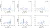 |
Fig. A.1 Determination of the size of the gaseous protocluster using various characteristic quantities for run B; the same values as in the left column of Fig. 5 are shown. The semimajor and semiminor axes of the ellipsoidal protocluster is plotted against time. Panels a)−c) use the infall over rotational velocity (W0) vs. weighted average radius |


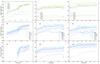 |
Fig. B.1 Same plot as that in Fig. 11 for other runs. From left to right are runs with tff/tvct = 0.4,1.1, and 1.5. Top panel: specific energy in various forms of the gas and sink components. Middle and bottom panels: dimensional energy analysis for gas and sinks respectively. |
All Tables
Simulation parameters: the cloud is specified with varying level of the ratio tff/tvct.
All Figures
|
Fig. 1 Zoomed images of run B at times 1.2, 2.4, and 2.8 Myr, showing the central dense objet. Upper panel: column density. Lower panel: velocity field overplotted on density sliced map. The origin of the coordinate corresponds to the center of the computational box and the figures are recentered such that the densest cell in the rightmost panel is at the center of the image. Sink particles are not shown. |
| In the text | |
|
Fig. 2 Zoomed images of run B at times 1.2, 2.4, and 2.8 Myr. Upper panel: column density. Lower panel: sink particles overplotted on column density. The circles represent the sink particles with the size proportional to the log of their masses and the arrows indicate their velocity. |
| In the text | |
|
Fig. 3 Zoomed images of run B at times 1.2, 2.4, and 2.8 Myr focusing on the central dense objet with two views showing the flattened shape. Upper panel: velocity field overplotted on density sliced map, edge-on view. Lower panel: velocity field overplotted on density sliced map, face-on view of the flattened rotating protocluster. |
| In the text | |
|
Fig. 4 Examples of the piecewise fit at nine time steps for the run with tff/tvct = 0.9. The normalized residual is plotted as function of cluster characteristic radius |
| In the text | |
|
Fig. 5 Time evolution of the semiaxes R and H of the ellipsoidal gas cluster in the left column. In the right column, the cluster mass is shown as function of time. The two curves represent the gas mass (dashed) and that plus the sink mass (solid) inside the ellipsoidal region defined with gas kinematics. From top to bottom are runs A, B, C, and D with increasing levels of turbulence. The protocluster size increases with turbulence level. Most of the mass is accreted onto the sinks while the cluster mass increases in time, therefore the gas mass stays roughly constant. |
| In the text | |
|
Fig. 6 Time evolution of the three semiaxes of the cluster determined with sink particles in the left column. The dashed curves and solid curves represent the values calculated with all sinks and the reduced values with distant sinks omitted, respectively. The sink mass (dashed) and total mass (solid) inside cluster region defined with sink distributions are plotted against time in the right column. The dotted line represents the sink mass before sink removal. Removing the sink particles far away from the center drastically reduces the size while only mildly decreasing the total mass. From top to bottom are runs A, B, C, and D with increasing levels of turbulence. |
| In the text | |
|
Fig. 7 Three semiaxes calculated from the rotational inertia matrix with the assumption of uniform mass distribution, plotted against Lcrit, which is the maximal allowed distance linking a member to the cluster. Examples are shown for four time steps of run B. |
| In the text | |
|
Fig. 8 Upper panel: gaseous protocluster mass-size relation defined with gas kinematics overplotted with measurements of star-forming clumps summarized by Fall et al. (2010, light gray dots) and Urquhart et al. (2014, dark gray dots). The total mass of the cluster is used (gas plus sinks). Lower panel: sink cluster number-size relation overplotted with embedded cluster concluded by Adams et al. (2006, dark gray dots) and Gutermuth et al. (2009, light gray dots). The gray line indicates the number-size relation R (pc) ∝ (N/ 300)1/2 by Adams et al. (2006). Simulations with four different levels of turbulent support are plotted. The blue solid, green dashed, red dot-dashed, and cyan dotted curves have virial parameters αvir = 0.12, 0.64, 0.96, 1.78, respectively. The curves represent the time sequence. As the protoclusters accrete, they gain in mass and move from left to right in the figure. Time steps before 2 Myr are plotted with thinner lines. |
| In the text | |
|
Fig. 9 Radius of sink clusters plotted against radius of gas protoclusters for four runs. The relations are plotted with thinner lines for time before 2 Myr and with thicker lines after 3 Myr. The color coding is the same as that in Fig. 8. The gas and sink cluster sizes show good correlation in general, while the sink cluster size is slightly smaller than that of the gas cluster. |
| In the text | |
|
Fig. 10 The specific angular momentum plotted against mass contained inside ellipsoids of varying radius at a series of time steps of run B. Solid curves represent the specific angular momentum of gas. Dashed curves represent the averaged value considering gas and sinks at the same time. The specific angular momentum of gas is more or less conserved during the collapse, which justifies our simplification, while the sink particles exhibit a loss in angular momentum. |
| In the text | |
|
Fig. 11 Top: different forms of specific energy of the cluster defined with gas kinematics plotted against time. The gas component is plotted in green and the sinks are plotted in yellow. The solid, dashed, dotted, and dash-dotted lines represent kinetic, gravitational, thermal, and magnetic energies respectively. The gravitational energy is plotted in absolute value. Middle and bottom: kinetic (blue) and gravitational energy (cyan) decomposition of the gas component (middle panel) and the sink component (bottom panel) of the protocluster plotted in specific values. Total energy, energy along z-axis, rotational energy, and energy perpendicular to z-axis are plotted with solid lines, dashed lines, dash-dotted lines, and dotted lines respectively. |
| In the text | |
|
Fig. 12 In solid curves for the gaseous protocluster and in dashed curves for the parent cloud, the PDF at several time steps for run B with tff/tvct = 0.9. The total mass of the protocluster is indicated in the legend. The normalization is performed such that the integral is equal to one. The distribution is close to lognormal at the beginning as a result of turbulence interaction. The gravity soon dominates and creates a prominent power-law tail. The slope −2.2 is the average of the cluster PDF slopes evaluated at the same density range as the black line except for the first time step. |
| In the text | |
|
Fig. A.1 Determination of the size of the gaseous protocluster using various characteristic quantities for run B; the same values as in the left column of Fig. 5 are shown. The semimajor and semiminor axes of the ellipsoidal protocluster is plotted against time. Panels a)−c) use the infall over rotational velocity (W0) vs. weighted average radius |
| In the text | |
|
Fig. B.1 Same plot as that in Fig. 11 for other runs. From left to right are runs with tff/tvct = 0.4,1.1, and 1.5. Top panel: specific energy in various forms of the gas and sink components. Middle and bottom panels: dimensional energy analysis for gas and sinks respectively. |
| In the text | |
Current usage metrics show cumulative count of Article Views (full-text article views including HTML views, PDF and ePub downloads, according to the available data) and Abstracts Views on Vision4Press platform.
Data correspond to usage on the plateform after 2015. The current usage metrics is available 48-96 hours after online publication and is updated daily on week days.
Initial download of the metrics may take a while.