| Issue |
A&A
Volume 589, May 2016
|
|
|---|---|---|
| Article Number | A36 | |
| Number of page(s) | 26 | |
| Section | Catalogs and data | |
| DOI | https://doi.org/10.1051/0004-6361/201526292 | |
| Published online | 11 April 2016 | |
Carbon stars in the X-Shooter Spectral Library⋆,⋆⋆,⋆⋆⋆
1
Observatoire Astronomique de Strasbourg, Université de Strasbourg, CNRS,
UMR 7550, 11 rue de l’Université
, 67000
Strasbourg,
France
e-mail:
This email address is being protected from spambots. You need JavaScript enabled to view it.
2
Kapteyn Astronomical Institute, University of
Groningen, Postbus
800, 9700 AV
Groningen, The
Netherlands
3
University of Vienna, Department of Astrophysics,
Türkenschanzstraße 17,
1180
Wien,
Austria
4
Dipartimento di Fisica e Astronomia Galileo Galilei, Università di
Padova, Vicolo dell’Osservatorio
3, 35122
Padova,
Italy
5
CRAL-Observatoire de Lyon, Université de Lyon, Lyon I, CNRS, UMR
5574, 69007
Lyon,
France
6
New York University Abu Dhabi, PO Box 129188, Abu Dhabi, UAE
7
Leibniz-Institut für Astrophysik Potsdam (AIP),
An der Sternwarte 16,
14482
Potsdam,
Germany
8
Instituto de Astrofísica de Canarias, vía Láctea s/n, La Laguna, 38205
Tenerife,
Spain
9
Departamento de Astrofísica, Universidad de La
Laguna, 38205 , La
Laguna, Tenerife,
Spain
10
Sterrenkundig Observatorium, Universiteit Gent,
Krijgslaan 281, 9000
Gent,
Belgium
11
Universidad Autónoma de Madrid, Departamento de Física
Teórica, 28049
Cantoblanco, Madrid, Spain
12
Instituto de Astrofísica, Facultad de Fisica, Pontificia
Universidad Catolica de Chile, Santiago 22, Chile
Received: 9 April 2015
Accepted: 20 December 2015
Abstract
We provide a new collection of spectra of 35 carbon stars obtained with the ESO/VLT X-Shooter instrument as part of the X-Shooter Spectral Library project. The spectra extend from 0.3 μm to 2.4 μm with a resolving power above ~8000. The sample contains stars with a broad range of (J − K) color and pulsation properties located in the Milky Way and the Magellanic Clouds. We show that the distribution of spectral properties of carbon stars at a given (J − K) color becomes bimodal (in our sample) when (J − K) is larger than about 1.5. We describe the two families of spectra that emerge, characterized by the presence or absence of the absorption feature at 1.53 μm, generally associated with HCN and C2H2. This feature appears essentially only in large-amplitude variables, though not in all observations. Associated spectral signatures that we interpret as the result of veiling by circumstellar matter, indicate that the 1.53 μm feature might point to episodes of dust production in carbon-rich Miras.
Key words: stars: AGB and post-AGB / stars: carbon / infrared: stars / ultraviolet: stars
Based on observations collected at the European Southern Observatory, Paranal, Chile, Prog. ID 084.B-0869(A/B), 085.B-0751(A/B), 189.B-0925(A/B/C/D).
Tables 1, B.1, E.1, E.2 are also available at the CDS via anonymous ftp to cdsarc.u-strasbg.fr (130.79.128.5) or via http://cdsarc.u-strasbg.fr/viz-bin/qcat?J/A+A/589/A36
The reduced spectra are only available at the CDS via anonymous ftp to cdsarc.u-strasbg.fr (130.79.128.5) or via http://cdsarc.u-strasbg.fr/viz-bin/qcat?J/A+A/589/A36
© ESO, 2016
1. Introduction
In the 1860s, Father Angelo Secchi discovered a new type of star – Type IV – known today as carbon stars (Secchi 1868). Carbon stars (hereafter C stars) are on the asymptotic giant branch (AGB) and have spectra that differ dramatically from those of K- or M-type giants. C stars are characterized by spectral bands of carbon compounds, such as CN and C2 bands, and by the lack of bands from oxides such as TiO and H2O. The classical distinction between carbon-rich and oxygen-rich stars is the ratio of carbon to oxygen abundance, C/O. If C/O > 1, oxygen is mostly bound to carbon in the form of carbon monoxide (CO) because this molecule has a high binding energy. As a result, little oxygen is left to form other oxides in these stellar atmospheres, whereas carbon atoms are available to form other carbon compounds.
Carbon stars are significant contributors to the near-infrared light of intermediate age stellar populations (1–3 Gyr) (e.g., Ferraro et al. 1995; Girardi & Bertelli 1998; Maraston 1998; Lançon et al. 1999; Mouhcine & Lançon 2002; Maraston 2005; Marigo & Girardi 2007). The absolute level of this contribution has an impact on mass-to-light ratios and has important implications for the study of star formation in the Universe. It is a matter of active research both on the theoretical side (e.g., Weiss & Ferguson 2009; Girardi et al. 2013; Marigo et al. 2013) and in the framework of extragalactic observations (e.g., Riffel et al. 2008; Kriek et al. 2010; Miner et al. 2011; Melbourne et al. 2012; Melbourne & Boyer 2013; Boyer et al. 2013; Zibetti et al. 2013). The quality of the photometric and spectroscopic predictions made by population synthesis models in this field depends on the existence of stellar spectral libraries, and their completeness in terms of evolutionary stages and spectral types.
Carbon stars contribute significantly to the chemical enrichment and to the infrared light of galaxies, but only small collections of C-star spectra exist to represent this emission (see Lloyd Evans 2010, for a review that includes earlier observations). As a reference for C-star classification, Barnbaum et al. (1996) published an extensive low-resolution optical spectral atlas (0.4–0.7 μm). It contains 119 spectra. Joyce (1998) provided a first impression of the near-infrared (NIR) spectra of C stars, again at low spectral resolution (48 spectra, with a spectral resolution of ~500). Repeated observations of single long-period variable (LPV) stars showed significant changes with phase, emphasizing the necessity of simultaneous observations across the spectrum. As NIR detectors improved, Lançon & Wood (2000) produced a library of 0.5–2.5 μm spectra of luminous cool stars with a resolving power R = λ/ Δλ ≃ 1100 in the NIR. It includes 25 spectra of seven carbon stars. Simultaneous optical spectra are available for 21 of them, but only at very low resolution (R ≃ 200). More recently, Rayner et al. (2009) have published the IRTF Spectral Library, which includes 13 stars of spectral type S (C/O = 1) or C. Their spectra have no optical counterparts, but extend from 0.8 μm as far as 5.0 μm at a resolving power R ~ 2000.
Observational properties of our sample.
Several population synthesis models have used the C-star collection of Lançon & Wood (2000) (Lançon et al. 1999; Mouhcine & Lançon 2002; Maraston 2005; Marigo et al. 2008). Lançon & Mouhcine (2002) suggested using a near-infrared color as a first-order classification parameter for the C-star spectra in these applications, but also noted that this disregards other potentially important parameters, such as the carbon-to-oxygen (C/O) ratio or the pulsation properties. One of the shortcomings of this data set is the narrow range of properties (Lyubenova et al. 2010, 2012). Another is that it simply contains too few stars to represent the variety of C-stars pectra.
In modeling of luminous cool stellar populations, two important sources of uncertainties (other than the incompleteness of spectral libraries) are the fundamental parameters assigned to the observed stars and the effects of circumstellar dust related to pulsation and mass loss on the upper asymptotic giant branch. Estimating effective temperatures, C/O ratios, and gravities requires a comparison with theoretical spectra. Loidl et al. (2001) showed that it is difficult to obtain a good theoretical representation of both the energy distribution and the spectral features, even for relatively blue C stars. Aringer et al. (2009) pointed out that static models without circumstellar dust cannot reproduce any NIR carbon star energy distribution with (J − K) > 1.6. Nowotny et al. (2011, 2013) computed small numbers of spectral energy distributions for pulsating models, at low spectral resolution. They reproduce the overall trend from optical carbon stars to dust-enshrouded sources, for which the whole spectrum is dominated by the emission from dust shells. But whether or not they reproduce the relationship between color and the depth of spectral features remains an open question. It is important to find out how dust shells may affect the optical and near-infrared spectra of C stars, especially for objects in the range 1.4 ≲ (J − K) ≲ 2 where the NIR luminosities of these AGB stars are large.
In this paper, we present spectra of 35 medium-resolution carbon stars extending from the near-ultraviolet through the optical into the near-infrared (0.3–2.5 μm). Although this collection is by itself not complete, it considerably extends the range of data available, and it offers unprecedented spectral resolution. We expect it to serve both the purpose of testing theoretical models for C-star spectra (Gonneau et al., in prep.) and of improving future population synthesis models. We describe the input stellar spectral library, our sample selection and the data reduction in Sects. 2 and 3. We discuss the spectra using a NIR color as a primary classification criterion in Sect. 4; in particular we discuss the appearance of a bimodal behavior of the spectral features and the overall spectral energy distribution in the redder C-star spectra. We define a list of spectroscopic indices in Sect. 5 that we use in Sect. 6 to quantify the spectral behavior and in Sect. 7 to compare our spectra with existing libraries of carbon-rich stars. We discuss our results in Sect. 8 and present our conclusions in Sect. 9.
2. The XSL carbon star sample
With X-Shooter (Vernet et al. 2011), the European Southern Observatory (ESO) made available a high-throughput spectrograph allowing the simultaneous acquisition of spectra from 0.3 to 2.5 μm, using two dichroics to split the beam into three wavelength ranges, referred to as arms: ultraviolet-blue (UVB), visible (VIS) and near-infrared (NIR). This simultaneity is invaluable when observing variable stars, and many C stars are LPVs (Lloyd Evans 2010).
Our team is building a large stellar spectral library under an ESO Large Programme, the X-Shooter Spectral Library (hereafter XSL, Chen et al. 2014). It contains more than 700 stars, observed at moderate resolving power (7700 ≤ R ≤ 11 000, depending on the arm) and covering a large range of stellar atmospheric parameters. The homogeneous spectroscopic extension into the near-infrared makes XSL unique among empirical libraries.
In this paper, we focus only on carbon stars. Table 1 gives a full description of the C-star sample. Table B.1 summarizes properties of these stars as available in the literature.
The sample includes stars from the Milky Way (MW) as well as from the Large and Small Magellanic Clouds (LMC, SMC). As C stars on the AGB form a relatively tight sequence in NIR color–color plots (2MASS, Skrutskie et al. 2006; DENIS, Epchtein et al. 1997; WISE, Wright et al. 2010; Whitelock et al. 2006; Nowotny et al. 2011), the primary aim of the selection was to sample an adequate range of near-infrared colors. This range was restricted to (J − K) < 3 to avoid stars with negligible optical flux. A few C stars with (J − K) < 1 are present in the sample, although these stars are considered too hot to be standard AGB objects; they are instead thought to have become carbon-rich through other processes, such as mass transfer from a companion.
While the effects of metallicity on stellar evolution tracks are large, leading to varying estimates of the fraction of C stars as a function of metallicity (Mouhcine et al. 2002; Mouhcine & Lançon 2003; Marigo et al. 2008; Groenewegen 2007), the effects of initial metallicity on the spectrum of a C star of a given color are relatively small based on static models (Loidl et al. 2001; Gonneau et al., in prep). Therefore, we initially consider all stars in the sample as one group, irrespective of the host galaxy.
A variety of LPV pulsation amplitudes and light curve shapes can be found in C stars with 1 ≲ (J − K) ≲ 3. A distinct period and a clear period-luminosity relation exist for large-amplitude variables (e.g., Whitelock et al. 2006), but many smaller-amplitude variables found in this range have extremely irregular light curves (see Hughes & Wood 1990). As shown in Figs. 1 and 2, there are systematic differences between the pulsation properties of our subsamples of C stars from the MW, the LMC and the SMC. On average, the LMC subset has a larger pulsation amplitude. More specifically, all the LMC stars in our sample display Mira-type pulsation, while the majority of the other stars in our sample are semi-regular variables, with comparatively small amplitudes (Table B.1). In addition, at a given color, the SMC stars tend to be brighter than their LMC counterparts (no reliable distances are available for the MW stars of the sample). These selection biases must be kept in mind when interpreting the spectra, which is another reason to treat the combined samples as one sample.
3. Data reduction
In the following section, we summarize the applied data reduction procedures. The carbon star data were acquired over ESO Periods 84, and 89 to 92 (Table 1). The narrow-slit widths for UVB, VIS and NIR images were 0.5′′, 0.7′′, 0.6′′, respectively.
3.1. UVB and VIS arms: extraction and flux-calibration
The UVB- and VIS-arm carbon star spectra observed in Period 84 are part of XSL Data Release I (DRI, Chen et al. 2014) and are used here unchanged. The basic data reduction for DRI was performed with X-Shooter pipeline version 1.5.0, up to the creation of rectified, wavelength-calibrated two-dimensional (2D) spectra. The extraction of one-dimensional (1D) spectra was performed outside of the pipeline with a procedure inspired by the prescription of Horne (1986). Observations of both the science targets and spectrophotometric standard stars through a wide slit (5.00′′) were used to obtain absolute fluxes (see Table 1 for exceptions).
We reduced UVB and VIS spectra from later periods with X-Shooter pipeline version 2.2.0 (Modigliani et al. 2010). For the purposes of this paper, the pipeline was also used for the extraction of 1D spectra and flux calibration. The choice of pipeline version does not affect our conclusions.
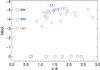 |
Fig. 1 Bolometric magnitudes and literature colors of our sample stars. The LMC stars (red triangles) are taken from Hughes & Wood (1990). The SMC stars (blue circles) are derived by Cioni et al. (2003). No reliable distances are known for the MW stars (black squares) of our sample. |
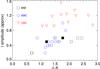 |
Fig. 2 I-band amplitudes of our sample stars. Symbols are as in Fig. 1. The amplitudes are estimated peak-to-peak variations. The values for LMC stars are taken from Hughes & Wood (1990). For the SMC stars, we estimated amplitudes using OGLE light curves (available through the Vizier service at CDS). For the MW, we estimated amplitudes based on K-band amplitudes by Whitelock et al. (2006); a value of 0.5 was assigned when no data were available. We note that for two MW stars (filled squares) large-amplitude luminosity dips are known to occur occasionally in addition to small-amplitude variations (the R CrB phenomenon). |
3.2. NIR arm: extraction
All NIR images were reduced with X-Shooter pipeline version 2.2.0, up to the creation of rectified, wavelength-calibrated 2D order spectra.
The extraction of 1D spectra was performed outside of the pipeline with a procedure of our own. A main driver for this choice was the need for more control over the rejection of bad pixels. The standard acquisition procedure for NIR spectra of point sources is nodding mode, with observations of the target at two positions (A and B) along the spectrograph slit.
Instead, we extracted A from (A−B) and B from (B−A) and combined them subsequently. Each extraction implements a rejection of masked and outlier pixels, as well as a weighting scheme based on a smooth throughput profile and on the local variance (see Appendix C for details). We note that the spectra in the extreme orders of the NIR arm display some residual curvature and broadening after pipeline rectification, which our profile accounts for in a satisfactory fashion. We then merged all the extracted orders to create a continuous 1D NIR spectrum.
Observations of program stars and of spectrophotometric standard stars through 5′′-wide slits, required for flux calibration, were reduced with pipeline sky subtraction switched off because residuals or negative flux levels were too frequent. The sky was estimated from both sides of the spectrum at the extraction of 1D spectra. We did not implement aperture corrections but used apertures as large as possible (considering the need to estimate the sky), sometimes at the expense of the signal-to-noise ratio of these wide-slit spectra. A number of the wide-slit observations of carbon stars lacked significant signal (especially in ESO Period P84; cf. Table 1), making it impossible to correct the higher resolution observations of these stars for slit losses.
3.3. Telluric correction and flux calibration
X-Shooter is a ground-based instrument. Therefore, we must correct our spectra for extinction by the Earth’s atmosphere. Standard flux calibration procedures account for continuous extinction, but not for molecular absorption lines (e.g., water vapour, molecular oxygen, carbon-dioxide, methane). Hereafter, we refer to these as telluric features. Telluric absorption features particularly affect the NIR arm and the reddest part of the VIS arm of X-Shooter.
3.3.1. VIS arm
The VIS spectra released in DR1 are already flux-calibrated and telluric corrected (Chen et al. 2014). For later periods, the flux calibration was performed within the X-Shooter pipeline. The telluric correction was applied afterwards. As for all cool stars in DR1, we selected telluric standard stars (with spectral types B and A) observed close in time and airmass to the carbon stars. We derived the telluric transmission spectra by removing the intrinsic stellar spectrum, e.g., fitting and removing H lines and normalizing the continuum. The science spectra were then divided by the transmission spectra.
Figure 3 shows some of the spectra of the carbon stars over a small part of the visible wavelength range (0.07 μm wide). The red spectrum is a telluric model, arbitrarily chosen, shown for comparison.
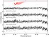 |
Fig. 3 Illustrative spectra in the VIS wavelength range. The red spectrum is a telluric sky model, smoothed to R ~ 10 000. From top to bottom, the stars are 2MASS J01003150-7307237, 2MASS J00571648-7310527, 2MASS J00493262-7317523 and 2MASS J00571214-7307045. Offsets of 0, 2, 4, 6 and 8 flux units have been applied to the C-star spectra and the telluric spectrum for display. |
3.3.2. NIR arm
The need for specific procedures to account and correct for telluric absorption is common to many NIR instruments. It is exacerbated in X-Shooter data by an unfortunate feature of the flat-field images. In the design of the pipeline, spectral features of the flat-field lamp remain present in the (globally) normalized flat-field images by which the data are divided and are propagated into the estimated instrument response curves. One such feature dominates over any other detector variations, a very strong and sharp bump in the K-band flatfielded spectra, with a much weaker secondary bump in the H-band (see, e.g., Fig. 9 of Moehler et al. 2014). At the altitude of the ESO Very Large Telescopes, water vapor absorption leaves broad gaps with no useable data in the NIR spectra, and only very few points anywhere that are free of any telluric molecular absorption. The interpolation of estimated response curves through these gaps is a particularly poorly constrained exercise in the case of X-Shooter pipeline products because only relatively high-order polynomials can match the bumps due to the flat-field. Therefore, we designed a method to evaluate the response curve that explicitly accounts for telluric absorption. Moehler et al. (2014) and Kausch et al. (2015) developed in parallel other implementations of this idea.
To model the telluric absorption, we chose to use the Cerro Paranal Sky Model, a set of theoretical telluric transmission spectra provided by J. Vinther and the Innsbruck team (Noll et al. 2012; Jones et al. 2013). These models are a more complete version of the spectra that can be found on the web application SkyCalc1,2.
The response curve was evaluated as follows. Because the flat-field bumps are variable in time, we required that the spectrophotometric standard star used to derive a response curve for a given program star was reduced with the same flat-field images as that program star. We then fit the flat-fielded spectrum of the flux standard with the product of the theoretical spectrum of this star, a telluric transmission model and the unknown response curve. Spectral regions with telluric features of intermediate depth were used to select the best-fitting telluric model within the available collection. The response curve was represented with a spline polynomial, with higher concentrations of spline nodes where required by the flat-fielding bumps. We corrected the response curve for continuous atmospheric extinction using the Paranal extinction curve, as available in the X-Shooter pipeline directory, and taking into account the airmass of the flux standard.
For the subsequent correction of the narrow-slit spectra of carbon stars, the search of the “best” telluric model is also needed and more important than above (as we care not only about the shape but also about the lines). Therefore, instead of using one telluric model, we allowed for a larger variety of telluric transmissions by using linear combinations of principal components of the available telluric absorption models, selected within a range of airmasses similar to the airmass of the data. We performed the χ2 minimization separately in four wavelength intervals3. The idea is to better target different molecules in the telluric spectra. Then, we divided the science spectrum by the telluric transmission and the response curve. We also corrected the science spectrum for continuous atmospheric extinction using the airmass at the time of observation.
Whenever possible, the final flux-calibrated spectra were absolutely flux-calibrated by using wide-slit (5′′) observations (refer to column “Flux note” of Table 1 for exceptions).
Figure 4 shows the quality of our telluric correction process on some of our carbon stars. The red spectrum shows a telluric model for comparison.
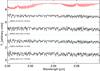 |
Fig. 4 Illustrative spectra in the NIR wavelength range. The red spectrum is a telluric sky model, smoothed to R ~ 8000. The stars are the same as in Fig. 3. |
3.4. Problem with the last order of NIR spectra
Some of our NIR observations, once flat-fielded, extracted, merged and flux-calibrated, display a step between the two reddest orders (around 2.27 μm, between orders 12 and 11). This could be related to a known vignetting problem in order 11, i.e., the last order of the NIR arm that covers 2.28–2.4 μm, to the high background levels in certain exposures, or to other unidentified artifacts. Although we account for variation in the background emission along the slit in order 11 and we reduce pairs of one flux standard and one carbon star with the same flat-field, we cannot eliminate the step completely.
We correct for the discontinuity, when present, by forcing the average flux level between 2.28 and 2.29 μm in order 11 to match the extrapolation of a linear fit to the spectrum between 2.150 and 2.265 μm. This choice is guided by the aspect of theoretical spectra of C stars (Aringer et al. 2009) and by published observations with other instruments (Lançon & Wood 2000; Rayner et al. 2009). Broad-band colors involving the Ks-band change by (usually much) less than 2% with this correction. The estimated extra uncertainty on measures of the 12CO bandhead within order 11 remains below a few percent for weak bands, but can reach 10% for some of the stars with strong CO bands.
3.5. Final steps
We use theoretical models of carbon stars (R ~ 200 000), computed specifically for this paper (based on the atmospheric mo-dels of Aringer et al. 2009), to shift the wavelength scale of our observed spectra to the vacuum rest-frame.
Finally, the three arms are merged to produce a complete spectrum from the near-UVB to the NIR4. The resolving power in the UVB, VIS and NIR ranges of the merged spectra are, respectively, R ~ 9100, ~11 000 and ~7770.
4. The diversity of carbon star spectra
Our sample of carbon stars presents quite a diversity in spectral shape and absorption-line characteristics. Figures D.1 to D.6 show our spectra from the UVB to the NIR wavelength range. The spectra were normalized to the flux at 1.7 μm and shifted for display purposes. The gray bands in the NIR mask regions where the telluric absorption is deepest and the signal cannot be recovered. It is important to note that the spectra were heavily smoothed to a common resolution (R ~ 2000) in these figures.
We group our carbon stars by (J − K) values when describing them in the remainder of this Section. Figure 5 summarizes the spectral variety of the sample, showing representative examples of each group. The colors are used to better identify the different groups.
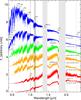 |
Fig. 5 Representative spectra from our sample of carbon stars. The gray bands mask the regions where telluric absorption is strongest. The areas hatched in black are those that could not be corrected for telluric absorption in a satisfactory way. The areas hatched in gray are the merging regions between the VIS and NIR spectra and between the last two orders of the NIR spectrum. In some spectra, data are missing at 0.635 μm. The spectra have been smoothed for display purposes to R ~ 2000. The colors represent the different groups of carbon stars. Group 1 stars are shown in blue (from top to bottom: HE 1428-1950 and Cl* NGC 121 T V8), Group 2 in red (2MASS J00571214-7307045), Group 3 in orange (from top to bottom: 2MASS J00542265-7301057 and SHV 0502469-692418) and Group 4 in red (from top to bottom: [ABC89] Cir 18 and SHV 0525478-690944). |
CO, CN and C2 produce the vast majority of features in spectra of carbon stars in this wavelength range. Some bands have sharp bandheads, but a forest of lines from various transitions are spread across the whole spectrum. The C2 Swan bands (Swan 1857) are dominant between 0.4 and 0.6 μm. Longward of 0.6 μm, the most prominent bandheads are due to CN. Note that the NIR CN bands, in particular the 1.1 μm bandhead, are also seen in M giants and supergiants (Lançon et al. 2007; Davies et al. 2013). The C2 band at 1.77 μm is one of the unambiguous characteristics of C stars in the NIR. The CO bands in the H and K windows are also present with varying strengths in all the spectra.
First we describe spectral characteristics of each group seen from visual inspection. We perform a more quantitative analysis in subsequent sections.
4.1. Group 1 – The bluest stars: (J – K) < 1.2 [5 stars]
Figure D.1 shows the five warmest C stars in our sample. The top two spectra of Fig. 5, displayed in blue, are representative of the two types of behaviors found in this group.
The top two stars of Fig. D.1, HD 202851 and HE 1428-1950, have spectra similar to those of early K type giants (CN band at 0.431 μm and G band of CH of similar strength, Hβ line in absorption). But they clearly display the C2 bands characte-ristic of C stars, in particular the Swan bands around 0.47 μm and 0.515 μm.
The three bottom spectra of Fig. D.1 have spectral energy distributions (SED) that peak at longer wavelengths, but have weaker molecular features in the optical range. The CN band at 0.431 μm and the G band of CH are undetectable in two of the three stars. On the other hand, the red system of CN is slightly stronger, and the NIR C2 bandhead (1.77 μm) and the CO bands are significantly stronger. Two of these three spectra display hydrogen emission lines, a phase-dependent signature of pulsation.
4.2. Group 2 – Classical C stars: 1.2 < (J – K) < 1.6 [7 stars]
Figure D.2 shows classical C stars: seven stars belong to this group. The third spectrum in Fig. 5 (2MASS J00571214-7307045), displayed in green, is representative of this group. All these C stars have 1.2 < (J − K) < 1.6. They happen to be located in the SMC, but we note that many of the Galactic C stars of Lançon & Wood (2000) would fall in this category.
At optical wavelengths, the Swan bands are the first features to appear when C/O > 1. Compared to the first group of spectra, the spectra collected here have significantly stronger absorption bands of CN and C2 in the NIR. C2 absorption modifies the spectrum across the J band and creates a strong bandhead at 1.77 μm. A forest of lines of both CN and C2 is responsible for the rugged appearance of the spectrum, which should not be mistaken as an indication of noise. CO bands in the H window appear weak, as a combined consequence of the C/O ratio and of overlap with many other features.
The SED and the H band (CO, C2, forest of CN and C2 lines) of the top spectrum of Fig. D.2 (2MASS J01003150-7307237) seem to indicate that this star is slightly warmer, or has a lower C/O ratio, than the others. The opposite holds for the last spectrum in that figure.
4.3. Group 3 – Redder stars: 1.6 < (J – K) < 2.2 [13 stars]
Figures D.3 and D.4 show redder stars. Thirteen stars compose this group. Group 3 is less homogeneous than Group 2: while some spectra simply seem to extend the sequence of Group 2 to redder SEDs with stronger features, others deviate from this behavior. This leads us to define two subgroups. A representative of each subgroup is included in Fig. 5 (see the fourth and fifth spectra, displayed in orange).
The stars that simply extend the behavior of group 2 have strong C2 bands in the J- and H-bands and weak CO bands. In two of these stars (T Cae and [W65] c2), the CO bands are re-latively stronger, suggesting a C/O ratio closer to 1 (cf. the S/C star BH Cru in Lançon & Wood 2000). We warn however that the interpretation of ratios of CO to other band strengths in terms of abundance ratios is a non-trivial exercise, as the band-strength ratios may depend on phase (see the multiple spectra of R Lep by Lançon & Wood 2000, or those of V Cyg from Joyce 1998).
Two stars stand out: SHV 0500412-684054 and SHV 0502469-692418. They are characterized by an absorption band around 1.53 μm (see Sect. 4.5), weaker C2 absorption, some of the strongest 2.3 μm CO absorption of this group, and a significantly smoother general appearance than other spectra. This latter property has, to our knowledge, never been emphasized before. In hindsight, it is also noticeable in previously published spectra that display the 1.53 μm feature (Lançon & Wood 2000; Groenewegen et al. 2009; Rayner et al. 2009).
Inspection of the spectra with the 1.53 μm feature also suggests that their emission in the red part of the optical spectra is relatively strong, considering their red NIR spectra. The spectra however drop rapidly to a negligible flux in the blue.
4.4. Group 4 – The reddest stars: (J – K) > 2.2 [9 stars]
The last two figures, Figs. D.5 and D.6, show our reddest stars. The dichotomy seen in Group 3 is obviously present here as well. The two bottom spectra from Fig. 5, displayed in red, are representative of that group, composed of nine stars. The general trend in this group is that the energy peak shifts from the optical to the near-infrared, which leads to a “plateau” in the K band of the reddest objects.
Properties of our spectroscopic indices.
It is interesting to note that at higher (J − K), more stars display the 1.53 μm absorption feature. The fact that the feature appears only in very red stars (but not in all very red stars) is consistent with previous observations (Joyce 1998; Groenewegen et al. 2009). The spectra that display 1.53 μm absorption share the properties already mentioned for their counterparts in Group 3. They clearly have a smoother appearance than the others. Unfortunately, the S/N ratio is poor for some of these objects beyond 2.25 μm. Where it is good, inspection by eye indicates that the CO bands in these smoother spectra have strengths similar to those in spectra with a forest of CN and C2 lines. In three cases, SHV 0520505-705019, SHV 0527072-701238, SHV 0528537-695119, there seems to be an excess of flux in the red part of the optical spectrum, compared to other stars.
4.5. The 1.53 μm feature
The 1.53 μm absorption feature was first noticed in cool carbon stars of the Milky Way (Goebel et al. 1981; Joyce 1998). These authors associated it with large-amplitude variability. The underlying molecules are most likely a combination of HCN and C2H2 (Gautschy-Loidl et al. 2004), and the 1.53 μm band is thought to be an overtone of the strong absorption band sometimes seen around 3 μm (e.g., in the spectrum of R Lep in the IRTF library). However, this correlation remains to be formally established, as Joyce (1998) stated that this correlation is poor.
In our sample, all the spectra that display the 1.53 μm feature belong to large-amplitude variables. The fact that in our sample they all happen to be in the LMC should be seen as a selection effect, since stars with this feature have previously been found both in the Milky Way and in dwarf galaxies more metal-poor than the LMC (e.g., the Sculptor dwarf, Groenewegen et al. 2009).
5. Spectroscopic indices for carbon stars
We derive spectroscopic indices from our flux-calibrated spectra to compare our sample with previous studies. Unless otherwise stated, we use the following formula to measure the strength of any absorption band X: ![Mathematical equation: \begin{eqnarray} I(X) = -2.5 \log_{10}[F_{\rm b}(X)/F_{\rm c}(X)], \label{eq_index} \end{eqnarray}](/articles/aa/full_html/2016/05/aa26292-15/aa26292-15-eq39.png) (1)where Fb(X) and Fc(X) are the mean energy densities received in the wavelength bin in the absorption band region and the (pseudo-)“continuum”5 of index X.
(1)where Fb(X) and Fc(X) are the mean energy densities received in the wavelength bin in the absorption band region and the (pseudo-)“continuum”5 of index X.
We note here that these “one-sided” indices depend on the quality of the flux calibration over moderate wavelength spans, in contrast to the classic “two-sided” Lick/IDS-type indices such as those defined by, e.g., Burstein et al. (1984), which are robust to small-scale flux-calibration issues. We evaluate error bars on indices by measuring them on spectra reduced with several estimates of the instrumental response curve, and by taking the standard deviation of these measurements.
Table 2 summarizes the properties of the bandpasses used to define our spectroscopic indices, as illustrated in Figs. 7–13.
5.1. Broad-band colors
For each of our spectra, we derived synthetic magnitudes using the Bessell (1990) filters R and I and the 2MASS filters (Cohen et al. 2003) J, H and Ks. We use these magnitudes to define the colors (R − H), (R − I), (I − H), (I − K), (J − H), (H − K) and (J − Ks).
Figure 6 compares our (J − Ks) colors with those found in the literature. When we exclude large-amplitude variables, we find a good agreement6. The dispersion increases with redder colors, as already noted by Whitelock et al. (2009). The large scatter for the large-amplitude pulsators is not surprising, since we are comparing our instantaneous color with 2MASS observations about ten years old, and many light curves display long term trends in addition to periodicity.
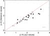 |
Fig. 6 Comparison of our (J − Ks) values with values found in the literature (2MASS values, Cutri et al. 2003). The red line indicates the one-to-one relation. The black points represent the stars with large-amplitude (I amplitude ≥0.8). The bar plotted in the bottom-right corner shows the ±1σ root-mean-square deviation of our photometry with respect to the literature (large-amplitude variables excluded). This is an upper limit of the uncertainties in the flux calibration and any possible residual variability. |
5.2. 12CO indices
We first look at the CO bands located in the K band. To measure the 12CO(2, 0) bandhead around 2.29 μm, we use the definition given by Kleinmann & Hall (1986): the absorption bandpass is centered on 2.295 μm (KH86c1) and the continuum bandpass is centered on 2.2899 μm (KH86CO1). We call this index CO12. Figure 7 shows these passbands on one of our spectra.
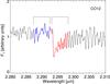 |
Fig. 7 Zoom into the 12CO(2, 0) feature near 2.3 μm. The red line indicates the region used to calculate the KH86CO1 bandpass, while the blue line corresponds to the KH86c1 bandpass measuring the continuum. This star is 2MASS J00571648-7310527. |
Other CO bands can also be found in the C-star spectra. Origlia et al. (1993) studied the CO band in the H-band near 1.62 μm, corresponding to Δυ = 3 ro-vibrational bands. In our spectra, this 12CO(6, 3) line does not always appear. Figure 8 shows two examples taken from our sample where the CO(6, 3) lines are seen (upper panel) or are hidden under a combination of CN and C2 lines (lower panel).
We define a new index COH, based on two other indices measuring the 12CO(5, 2) at 1.60 μm (COH52) and the 12CO(6, 3) line at 1.62 μm (COH63):  (2)
(2)
5.3. 13CO index
The strongest 13CO features in the spectra are the Δυ = 2 ro-vibrational bands located around 2.53 μm. To measure the 13CO(2, 0) bandhead, we use the definition of the bandpass centered on 2.3462 μm given by Kleinmann & Hall (1986) (KH86CO3). We do not use the same definition for the continuum as their bandpass is centered on 2.2899 μm and thus too far away from the absorption bandpass and more likely to be sensitive to slope effects. Therefore, we define a new bandpass for the continuum and create the index CO13. Figure 9 shows the definition of the bands used to define this index on one of our spectra.
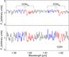 |
Fig. 8 Zoom into the 12CO(6, 3) line near 1.62 μm. The red lines indicate the features regions, while the blue measure the continuum. The upper panel shows the spectrum of a carbon star, Cl* NGC 121 T V8, in which the 12CO(5, 2) and 12CO(6, 3) bands are visible. The lower panel corresponds to another carbon star, 2MASS J00571214-7307045, in which the CN and C2 lines are more prominent and overlap with the CO lines. The spectra have been normalized at 1.62 μm for display purposes. |
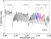 |
Fig. 9 Zoom into the 13CO(2, 0) line near 2.35 μm. The red line indicates the region used to calculate the KH86CO3 bandpass, while the blue line corresponds to the KH86CO2 bandpass measuring the continuum. This star is SHV 0500412-684054. |
5.4. CN index
CN is also seen in carbon-rich spectra. The red system of CN appears beyond 0.5 μm and the bands grow towards longer wavelengths. To estimate the CN in the NIR part of the spectrum, we use rectangular filters adapted from the 8-color system of Wing (1971). We use an index CN, based on Wing’s W110 and W108 passbands, that measures the CN feature at 1.1 μm. Figure 10 shows these passbands.
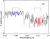 |
Fig. 10 Zoom into the CN line near 1.1 μm. The red line indicates the region used to calculate the W110 bandpass, while the blue line corresponds to the W108 bandpass measuring the continuum. This star is SHV 0502469-692418. |
5.5. Measure of the 1.53 μm feature
Some of our stars exhibit the 1.53 μm feature. We interpret this feature to be caused by HCN+C2H2. We define an index DIP153 to measure its depth. Figure 11 shows two examples taken from our sample where this feature is seen (upper panel) and absent (lower panel).
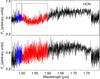 |
Fig. 11 Zoom into the HCN+C2H2 lines around 1.53 μm. The upper panel shows an example of a carbon star, SHV 0502469-692418, in which the HCN+C2H2 feature is visible. The lower panel corresponds to another carbon star, T Cae, in which the feature is missing. The red line indicates the region used to calculate the absorption bandpass, while the blue line corresponds to the continuum bandpass. |
5.6. C2 indices
C2 bands appear at many wavelengths in the spectra of carbon stars. The bands between 0.4 and 0.7 μm correspond to the Swan system (Swan 1857). The C2 bands at 0.77, 0.88, 1.02 and 1.20 μm are part of the Phillips system (Phillips 1948).
The Ballik-Ramsay fundamental band is the C2 band at 1.77 μm (Ballik & Ramsay 1963). To measure it, we use the same definition as Alvarez et al. (2000). The bandpasses used to define the C2 index are shown in Fig. 12.
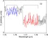 |
Fig. 12 Zoom into the C2 line around 1.77 μm. The red line indicates the region used to calculate the C2_band bandpass, while the blue line corresponds to the bandpass measuring the continuum. This star is 2MASS J00563906-7304529. |
The upper-right panel of Fig. 13 shows the C2 Swan system for one of our spectra. Due to low signal-to-noise for the XSL carbon stars at short wavelengths, the bands near 0.47 μm or bluer are barely seen. The band near 0.56 μm is problematic because of instrumental issues in that range (Chen et al. 2014), and the bands above 0.6 μm are too heavily contaminated by CN. This leaves the band near 0.5165 μm as our best choice to define an index, even though this index cannot be defined for all stars of our sample due to an absence of signal in the UVB/VIS parts of some of our spectra. We call this index C2U.
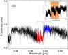 |
Fig. 13 The C2 Swan system (top panel) and a zoom into the C2 line around 0.5165 μm. The red line indicates the region used to calculate the C2U_band bandpass, while the blue line corresponds to the C2U_cont bandpass measuring the continuum. This star is HE 1428-1950. |
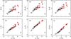 |
Fig. 14 Some color–color plots derived from our sample of carbon stars. The red circles stand for carbon stars showing the 1.53 μm feature. For the R filter, we adopt some conservative values. The bars plotted in the bottom-right corners are determined as in Fig. 6. |
5.7. Measure of the high-frequency structure
We also estimate the high-frequency structure in the H and K bands, inspired by the smooth appearance of the NIR spectra of C stars with the 1.53 μm feature. For both windows, we first fit a straight line on the wavelength range under study: 1.66–1.7 μm for the H band and 2.18 – 2.23 μm for the K band. We then divide our spectrum by this fit, thus normalizing the continuum. Next, for any window X, we derive the rms from the following formula: 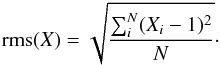 (3)
(3)
6. Results
6.1. Color–color plots
Figure 14 shows the locus of the observed carbon stars in color–color diagrams, based on the measurements made in Sect. 5.1. On the whole, different colors are well correlated with each other. The dispersion along the trend is smaller at bluer colors.
The red circles stand for carbon stars showing the 1.53 μm feature in their spectra. A trend characterizes these stars in the color–color diagrams: at a given (J − Ks), they are bluer when looking at color indices that involve R or I. We note that only panels b, c, e and f show colors that include the H band, which hosts the 1.53 μm feature itself. The separation between stars showing the 1.53 μm feature and classical C stars, however, is present in all the panels.
This separation into two groups reflects the results of visual inspection in Sect. 4. Stars with the 1.53 μm feature tend to have excess flux at the red end of the optical spectrum, for a given energy distribution at farther NIR wavelengths.
6.2. Molecular indices versus color
Figure 15 shows all the indices previously defined as a function of (J − Ks). For each group of (J − Ks) (cf. Sect. 4), we calculate the average values of each index and display them as filled symbols. The error bars indicate the 1σ standard deviations. We separate the red C stars from Groups 3 and 4 into two sub-groups: those with the 1.53 μm feature and those without.
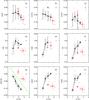 |
Fig. 15 Some indices derived from our sample of carbon stars as a function of (J − Ks). The red circles stand for the carbon stars with the 1.53 μm feature. The filled diamonds represent the averaged values of our indices as a function of the bin number based on (J − Ks), and the bars measure the dispersion within bins. Typical uncertainties on individual measurements are shown in purple. |
Panels a to c in Fig. 15 display the CO indices as a function of (J − Ks). The data points are highly dispersed, with a marginal trend of decreasing 12CO indices when (J − Ks) increases.
In the H-band, the prominence of the CO bands in carbon star spectra depends on the strength of the CN and C2 bands. These, in turn, depend on effective temperature, but also on the C/O ratio (Fig. 3 of Loidl et al. 2001). While strong in S and S/C stars (Rayner et al. 2009; Lançon & Wood 2000), the H-band CO features become indistinguishable in the forest of CN and C2 lines at large C/O. In addition, the CO band strengths anticorrelate with surface gravity (Origlia et al. 1993). In view of the many parameters that may control the amplitude of the related dispersion of COH values (others could include metallicity, microturbulence, convection), our sample is too small to consider the trend with (J − Ks) significant.
At 2.29 μm, contamination by features other than CO is reduced but not negligible. Again, we believe the trend with (J − Ks) is only marginal. Anticipating later discussions, it is interesting to note that two of the stars with the 1.53 μm feature are among those with the highest values of CO12.
Our measurements of 13CO approach 0 above (J − Ks) ≃ 2, and its detection is only significant in a few relatively blue stars. To some extent, this results from contamination of the measurement bandpasses by a forest of lines from other molecules and to measurement uncertainties beyond 2.25 μm. But weak 13C abundances are also a natural and well known result of the third dredge-up, which brings freshly synthesized 12C to the surface (Lloyd Evans 1980; Bessell et al. 1983).
Panel d shows the result for the CN index. The behavior is not monotonic. First, the strength of the CN index increases, up to (J − Ks) ≃ 1.6. Then, for redder stars, the CN bandhead slowly fades. For stars with (J − Ks)≥ 2, the sources with the 1.53 μm absorption feature are clearly separated from the classical carbon stars.
Panels e and f display the C2 indices. The C2U index is not defined for the reddest objects in the sample because of a lack of signal at the relevant short wavelengths. The strength of both C2 indices increase with increasing (J − Ks) and drop down for the reddest (J − Ks) values. The stars with the 1.53 μm absorption feature behave differently (weaker C2 bands, for a given (J − Ks)).
Panel g shows the index measuring the strength of the 1.53 μm feature as a function of (J − Ks). There is a clear separation between stars with the 1.53 μm feature (red points) and the others. We add a green line showing this separation for later comparisons.
The last two panels h and i display the results for the measure of the high-frequency structure in the H and K bands. The contribution of observational errors to the measured rms indices is in general smaller than 0.02. As expected, the values of the rms increase with increasing (J − Ks), but stars with the 1.53 μm feature follow the opposite trend. The quantitative assessment supports the conclusion drawn from visual inspection (see Figs. D.1 and following).
7. Comparison with the literature
Figures 16 and 17 compare our sample of carbon stars with existing libraries.
7.1. Spectra from Lançon & Wood (2000)
A widely-used library containing carbon stars is that constructed by Lançon & Wood (2000, hereafter LW2000). They built a library of spectra of luminous cool stars from 0.5 to 2.5 μm, which includes 7 carbon stars. In addition, their data include multiple observations of individual variable stars. One of their stars, R Lep, is a large-amplitude variable star, which exhibits the 1.53 μm feature. The different observations of this star are represented as filled magenta stars in Figs. 16 and 17.
7.2. Spectra from Groenewegen et al. (2009)
We also compare our spectra with spectra observed by Groenewegen et al. (2009). They observed carbon rich AGB stars in the Fornax and Sculptor dwarf galaxies. The observations covered the entire J- and H-band atmospheric windows. This sample is particularly interesting as their color-selected sample happened to contain several carbon stars with the 1.53 μm feature. Table 3 summarizes properties of their carbon stars: 2MASS J, H and Ks magnitudes and also the strength of the 1.53 μm feature, as available from Table 1 of Groenewegen et al. (2009). Based on their classification, stars for which this feature is “medium,” “strong” or “extreme” are represented as filled blue triangles in Figs. 16 and 17.
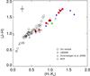 |
Fig. 16 The spread of our sample of carbon stars (circles) in the (J − H)–(H − Ks) color–color plane. The star symbols represent LW2000, the triangles represent Groenewegen et al. (2009) and the squares represent IRTF. Colored symbols stand for those carbon stars with the 1.53 μm feature. |
7.3. Spectra from IRTF (Rayner et al. 2009)
Finally, we compare our carbon stars with those from the IRTF Spectral Library (Rayner et al. 2009, hereafter IRTF). Their collection counts 8 C-star spectra from 0.8 to 5.0 μm, including R Lep. In Figs. 16 and 17, this star is represented as a filled green square.
7.4. Results
Figure 16 shows the color–color diagram of (J − H) versus (H − Ks) for our sample of carbon stars (circles), to which we add the C stars from LW2000 (stars), Groenewegen et al. (2009) (triangles) and IRTF (squares). The colored symbols represent the carbon stars with the 1.53 μm feature. All the colors, except those from Groenewegen et al. (2009), were rescaled to 2MASS values for consistency in our comparison7. It is interesting to note that the 1.53 μm feature makes the stars fainter in H, so stars with this feature are bluer in (J − H) and redder in (H − Ks).
We compute for the three samples of carbon stars under study the spectroscopic indices just like for the XSL spectra. Figure 17 shows six of our indices as a function of (J − Ks). Not all the indices are defined for the stars from Groenewegen et al. (2009), as their spectra are confined to the J and H bands.
Panel a shows the result for the CN index. The trend is as in Fig. 15: an increase of the CN band up to (J − Ks) ≃ 1.6 and then a slow decrease at redder colors.
Panel b shows the result for the DIP153 index. The green line is the same line as in panel g of Fig. 15. Our criterion to identify stars with the 1.53 μm feature appears to be reasonable when applied to a larger sample.
In the same panel, one star identified with a star symbol and not explicitly identified as containing HCN+C2H2 appears close to the group of stars with the 1.53 μm feature. This star is BH Cru, a Galactic star, with spectral type CS. Its IRAS-LRS spectrum shows that it is not surrounded by a lot of dust (“a hint of circumstellar emission” as mentioned by Lambert et al. 1990). This star displays exceptionally strong CO bands in the H-band and these contaminate the DIP153 index (see Fig. B28 of Lançon & Wood 2000).
Panel c plots the COH index. We still observe a decrease of the strength of the COH as (J − Ks) increases.
Panel d shows the C2 index. The most of the “normal” stars seem to lie on a sequence, while the stars with this 1.53 μm feature are all gathered in the lower right-hand quarter of the plot.
Panels e and f display the CO12 and CO13 indices. The general trend is a decrease of those two indices as (J − Ks) increases.
8. Discussion
8.1. The bluest stars
In Sect. 4.1, we described the 5 bluest carbon star spectra of our sample (Fig. D.1). For the top two stars, HD 202851 and HE 1428-195, effective temperatures available in the literature are above 4500 K (Bergeat et al. 2002; Placco et al. 2011). Hence these are unlikely to be classical C stars on the AGB. Formation scenarios with mass transfer from binary companion are more plausible.
The other three stars of the group (Cl* NGC 121 T V 8, SHV 0518161-683543 and SHV 0517337-725738) cannot be modeled as reddened versions of the previous two with standard reddening laws. The energy distributions do not match, and in addition circumstellar dust is not expected to play a major role around stars this warm. These three stars are intrinsically redder than the first two and most likely do belong to the AGB. Only a detailed comparison with models will provide estimates of their parameters (Gonneau et al., in prep.). A redder SED can indicate a cooler effective temperature. Differences in the depth of the molecular bands can be the result of different metallicities and/or C/N/O abundance ratios. Luminosity may also play a role as the strengths of the CO and CN bands tend to increase when surface gravities drop.
One might be tempted to consider environmental effects, as the bottom three spectra of Fig. D.1 belong to stars in the Large and Small Magellanic Clouds while the top two are in the Milky Way. But one of the two top spectra belongs to a Galactic Halo star (HE 1428-1950, Goswami et al. 2010), and is likely also of subsolar metallicity (Kennedy et al. 2011). It is unknown to which MW population the second top star belongs.
Finally, we note that two of these five spectra clearly display Hβ in absorption, and two others Hβ in emission. Hydrogen deficiency is unlikely to be an important characteristic of any of the stars in this group. Hydrogen emission is a known transient property of pulsating variables, usually interpreted as the results of shocks in the extended atmospheres.
Carbon stars from Groenewegen et al. (2009).
8.2. The bimodal behavior of red carbon stars
The previous sections have pointed out a bimodal behavior among carbon stars with redder near-infrared colors. The presence or absence of the 1.53 μm absorption feature separates the two types of behaviors (at least in the XSL sample).
Figure 18 shows two of our high-resolution C-star spectra with similar (J − Ks) (of ≃1.85). The 1.53 μm feature is present in the top spectrum but not in the bottom one. In addition to the HCN+C2H2 feature, the top spectrum shows a smoother near-infrared spectrum and an energy distribution with two components, one peaking at red optical wavelengths, the other at long wavelengths.
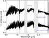 |
Fig. 18 Two high-resolution, high signal-to-noise ratio C-star spectra for which (J − Ks) ≃ 1.85. Only the top spectrum exhibits the 1.53 μm feature. It also appears smoother in the near-infrared than the bottom one, and it has a peculiar energy distribution. The gray bands mask the regions where telluric absorption is strongest. The areas hatched in black are those that could not be corrected for telluric absorption in a satisfactory way. The areas hatched in gray are the merging regions between the VIS and NIR spectra, and between the last two orders of the NIR part. |
What might explain this bimodal behavior? Groenewegen et al. (2009) have already discussed the anti-correlation between the strength of the 1.53 μm feature and the C2 bandhead at 1.77 μm. As the 1.53 μm feature is likely carried in part by C2H2, they have suggested the formation of this complex molecule occurs at the expense of C2 when the C/O ratio and the physical conditions are appropriate. While we have no argument against this suggestion, other parameters are needed to explain the effects we see in the overall SED and the anti-correlation with the apparent strength of the forest of lines in the H- and K-bands.
Two of the main fundamental parameters of carbon star mo-dels are the effective temperature and the C/O ratio. Aringer et al. (2009) showed that dust-free hydrostatic models with any reasonable values for these parameters fail to reproduce stars redder than (J − Ks) ≃ 1.6. Circumstellar dust is invoked to explain redder objects. At optical and NIR wavelengths, this dust is usually thought of as a cause of extinction (Lançon & Mouhcine 2002; Lloyd Evans 2010). But extinction by itself cannot explain the phenomenon we observe. All classical extinction laws are monotonic functions of wavelength through the optical and NIR range. They cannot explain that, at a given (J − Ks), stars with the 1.53 μm feature have an apparent peak in their Fλ energy distribution in the red part of the optical spectrum.
One explanation for both the SED and the apparent smoothness of the peculiar spectra in the NIR range (e.g., SHV 0500412-684054) is an additional continuous emission component at NIR wavelengths. While the emission component of the veiling by circumstellar dust is usually detected only at longer, mid-infrared wavelengths for mass-losing AGB stars, the particular instantaneous structure around some stars may lead to a significant contribution in the near-infrared. An additive continuum reduces the equivalent width of absorption features in the composite spectrum, resulting in a smoother appearance. Indeed, such a dilution is seen at NIR wavelengths in some of the spectra of dusty pulsating C-star models of Nowotny et al. (2011, 2013), although this aspect was not pointed out by the authors. Furthermore the existence of objects dominated by dust emission at NIR wavelengths such as V CrA (Fig. A.2) hints at intermediate situations.
If we accept the idea of continuous thermal dust emission in the NIR, we should expect all near-infrared photospheric molecular bands to be similarly weakened. That would explain the weaker C2 and CN bands. The stronger HCN+C2H2 absorption suggests that these molecules are intermixed with the dust high above the region responsible for the other absorption bands. A similar argument was made by Sloan et al. (2006) and Zijlstra et al. (2006). As the CO bands around 2.3 μm do not seem to be weakened as much as the C2 or CN lines, CO is also inferred to exist at circumstellar radii at least as large as the emitting dust. This is compatible with dynamical models of carbon star atmospheres, which indicate that the robust CO molecule exists throughout the circumstellar environment, and the CO(2, 0) lines originate around the radii of dust production, i.e., where most of the NIR dust emission is likely to be produced (Nowotny et al. 2005).
Indeed, for dust to emit at NIR wavelengths, it must be relatively hot and located near the star. This is most likely to happen when the dust first forms, and to last only until that dust shell is carried farther out into cooler regions. Why the presence of dust emission seems to correlate so well with the presence of the 1.53 μm feature would remain to be explained by a renewed look at models of the chemical structures of pulsating atmospheres.
It is also interesting to note that all the stars in our sample with the 1.53 μm absorption band are Miras8 but not all the Miras have this feature (see Table B.1 for more details). Large-amplitude pulsation might thus be a requirement for dust to be forming via a particular chanel, associated with the NIR signatures of HCN and C2H2 and with relatively hot dust temperatures.
Sloan et al. (2015) and Reiter et al. (2015) recently emphasized another example of the connection between the spectral properties and the pulsation mode of carbon stars: the long period variables separate into two sequences when plotting the mid-infrared [5.8]–[8] color versus (J − Ks). Nearly all semi-regular variables (SRV) follow a blue sequence with (J − Ks) ≲ 2, while Miras dominate a redder sequence. In the range of overlap, around (J − Ks) ≃ 1.8, SRVs have larger [5.8]–[8] color indices than Mira variables, which the authors relate to the presence of a strong C3 absorption band around 5 μm in SRVs. The competition between C3, C2, HCN, and C2H2, as well as the relations between their abundances, their band strengths, the stellar pulsation amplitude, and the instantaneous atmospheric structure, are interesting open questions for future statistical studies.
Finally, we note that this discussion does not account for the effects of circumstellar kinematics on line profiles. Velocity differences larger than 15 km s-1 within the molecular line formation regions of long-period variables lead to complex broadened line profiles (Nowotny et al. 2005), which will affect spectra observed at the resolution of X-Shooter. This has been explored theoretically over small wavelength ranges only, and at very high spectral resolution. More extensive calculations are needed to evaluate to what extent the velocity profiles in large-amplitude variables may contribute to a smoother appearance of some spectra. However, because the apparent smoothing of spectra with 1.53 μm absorption was detectable in data taken at R ≤ 2000 (Lançon & Wood 2000; Groenewegen et al. 2009; Rayner et al. 2009), we anticipate that velocity broadening will not by itself explain all the observations.
8.3. Synthetic stellar populations with carbon stars
This collection of spectra of carbon stars offers several improvements over previous collections for the simulation of spectra of intermediate age stellar populations. It extends the collection of Lançon & Wood (2000) to bluer stars and provides higher resolution at optical wavelengths. It also offers a new insight into the importance of evolutionary parameters such as surface composition, pulsation properties and mass loss along the AGB.
The contributions of TP-AGB and C stars are largest in populations with a significant component of intermediate-age stars, such as intermediate-age star clusters (contributions of the order of 50% in the K band; Ferraro et al. 1995; Girardi et al. 2013) or galaxies with a strong post-starburst component (Lançon et al. 1999; Miner et al. 2011; but see Kriek et al. 2010 and Zibetti et al. 2013 for counter-examples). Melbourne et al. (2012) use star counts to show the contribution of TP-AGB stars reaches 17% at 1.6 μm in a sample of local galaxies, but they do not separate O-rich and C-rich stars. In near-infrared color-magnitude diagrams of the Magellanic Clouds, a densely populated plume of C stars extends from (J − K) = 1.2 to (J − K) = 2 at its bright end (Nikolaev & Weinberg 2000). The corresponding contribution to the light at 2 μm amounts to 6–10% of the total, and is similar to that of O-rich TP-AGB stars (Melbourne & Boyer 2013).
Many of the C stars detected in the above populations are in the range of colors for which we have found bimodal spectral properties. It will be necessary to evaluate proportions of C stars of the two types in the future, based on models and observations. As we have found that only large-amplitude pulsators in current samples display the 1.53 μm feature and the associated spectral properties, this implies that future detailed population synthesis models will need to include the prediction of pulsation properties more routinely than is currently the case. However, considering the above assessments of the weight of C stars in spectra of galaxies, approximate proportions will be sufficient for many purposes. Demand for precision will come, for instance, when the next generation of extremely large telescopes will produce detailed near-infrared observations of star clusters in samples of remote galaxies.
In the short term, the spectra of this paper will be compared with stellar models, with the double purpose of validating those models and of constraining the location of the observed stars along stellar evolution tracks. The X-Shooter archive contains additional C-star spectra that should be added to the XSL collection in the future. O-rich stars on the AGB are also included in XSL. They should be compared with those of LW2000 and included in the TP-AGB modeling procedures.
9. Conclusions
We have presented a new collection of spectra of carbon stars, observed at medium resolution and covering wavelengths from the near-ultraviolet to the near-infrared.
Our sample is quite diverse. We point out a bimodal behavior among the spectra with (J − K) larger than 1.6. In addition to the “classical” carbon star features, which are due predominantly to CN, C2, and CO, a subset of our stars also displays an absorption band at 1.53 μm. These tend to have a smoother spectral appearance. In our sample, all the stars with the 1.53 μm feature are large-amplitude (Mira-type) variables. On the other hand, not all the Mira-type pulsators display that feature or the associated properties.
Our interpretation is that red carbon stars are enshrouded in circumstellar dust they have produced, which causes veiling (Nowotny et al. 2011, 2013). The apparent weakening of the forest of photospheric molecular lines, such as those of CN, could occur in specific circumstances, when some of the dust is warm enough for the veiling to include a significant continuous emission component in the near-infrared. The 1.53 μm feature, which is most likely carried by HCN and C2H2, could be produced in cool parts of the photospheres or could be distributed within the dusty circumstellar environment.
A comparison with dynamical models, i.e., models including pulsation, dust formation, and mass loss, is needed to confirm and clarify this picture. Indeed, other mechanisms may play a role. For instance, the interplay between radiative transfer and dynamics could matter as it changes individual line profiles (Nowotny et al. 2005; Eriksson et al. 2014). If the velocity distributions within the thick photospheres of pulsating stars are broad enough, a measurable smoothing of the spectra could occur. It will also be interesting to compare the near-infrared findings with observations at longer wavelengths where the spectral properties of carbon stars have also been shown to depend on the variability type (Sloan et al. 2015; Reiter et al. 2015).
This collection of spectra will contribute to the improvement of stellar population synthesis models. Before using them, it is necessary to estimate the corresponding fundamental stellar parameters such as effective temperature or surface gravity. In a companion paper, we compare the observations with predictions from hydrostatic models, and provide such estimates for spectra which are not affected too strongly by pulsation. For strongly pulsating stars, high-resolution spectra across a wavelength range as broad as that observed with X-Shooter remain to be calculated.
The files were computed with version 1.2 based on SM-01 Mod1 Rev.74, LBLRTM V12.2, and the line database was aer_v_3.2.
We use the following wavelength regions: 0.9–1.345 μm, 1.46–1.8 μm, 1.975–2.1 μm and 2.1–2.5 μm.
The three arms overlap quite well: UVB: 0.3–0.59 μm; VIS: 0.53–1.02 μm; NIR: 0.99–2.48 μm.
At the resolution of our C-star spectra, the true continuum is inaccessible anywhere. What we call pseudo-“continuum” in this section is simply a reference flux level measured outside the molecular band of interest for a particular spectrophotometric index, following earlier usage by, e.g., Worthey et al. (1994).
The offset might be due to zero-point differences between our synthetic photometry and the listed 2MASS magnitudes. Indeed, using the reference fluxes for zero-magnitude stars in Cohen et al. (1992) and a recent template Vega spectrum from the Hubble Space Telescope calibration documentation (ftp://ftp.stsci.edu/cdbs/current_calspec/), our synthetic photometry gives (J − Ks) = 0 for Vega, while the 2MASS point source catalog lists (J − Ks) = − 0.31 for that star.
The colors were rescaled by the following factors: (J − H)new = (J − H)ori − 0.10; (H − Ks)new = (H − Ks)ori − 0.05; (J − Ks)new = (J − Ks)ori − 0.15.
This is also the case for the stars with 1.53 μm absorption observed by Goebel et al. (1981), Joyce (1998), Lançon & Wood (2000). Among the 9 C stars in Groenewegen et al. (2009) with this absorption and with some amplitude information (mostly from Whitelock et al. 2009) at least four are Miras. Two are labeled “semi-regular with long term trends”, three others have quoted J-band amplitudes of 0.6, 1.0 and 1.0 in that article.
C-R stars, as defined in the older carbon-star classification, are usually extrinsic carbon stars (Alksnis et al. 1998).
Acknowledgments
We thank the referee, Dr. Greg Sloan, for the thorough and detailed review that helped to improve the quality of this paper. We also thank C. Loup, M. Allen, R. Ibata, M. Groenewegen, and J. van Loon for helpful discussions. We would also like to thank to A. Modigliani, S. Moehler, J. Vinther, and the ESO staff for their help during the XSL observations and reduction process. The authors acknowledge financial support from PNPS, “Programme National de Physique Stellaire” (Institut National des Sciences de l’Univers, CNRS, France) and from NOVA, the Netherlands Research School for Astronomy for support. B.A. acknowledges the support from the project STARKEY funded by the ERC Consolidator Grant, G.A. n. 615604. This research was funded by the Austrian Science Fund(FWF): P21988-N16. J.F.-B. and A.V. acknowledge support from grant AYA2013-48226-C3-1-P from the Spanish Ministry of Economy and Competitiveness (MINECO). This research has made use of the VizieR catalogue access tool and of the Simbad database, both operated at CDS, Strasbourg, France. We acknowledge the variable star observations from the AAVSO International Database contributed by observers worldwide and used in this research, especially the BAAVSS.
References
- Aaronson, M., Bothun, G. D., Budge, K. G., et al. 1988, IAU Symp., 130, 185 [NASA ADS] [Google Scholar]
- Aaronson, M., & Mould, J. 1985, ApJ, 290, 191 [NASA ADS] [CrossRef] [Google Scholar]
- Alcock, C., Allsman, R. A., Alves, D., et al. 1996, MNRAS, 280, L49 [NASA ADS] [Google Scholar]
- Alksnis, A., Balklavs, A., Dzervitis, U., & Eglitis, I. 1998, A&A, 338, 209 [NASA ADS] [Google Scholar]
- Alksnis, A., Balklavs, A., Dzervitis, U., et al. 2001, Balt. Astron., 10, 461 [NASA ADS] [Google Scholar]
- Alvarez, R., Lançon, A., Plez, B., et al. 2000, A&A, 353, 322 [NASA ADS] [Google Scholar]
- Aringer, B., Girardi, L., Nowotny, W., et al. 2009, A&A, 503, 913 [NASA ADS] [CrossRef] [EDP Sciences] [Google Scholar]
- Ballik, E. A., & Ramsay, D. A. 1963, ApJ, 137, 61 [NASA ADS] [CrossRef] [Google Scholar]
- Barnbaum, C., Stone, R. P. S., & Keenan, P. C. 1996, ApJS, 102, 1181 [Google Scholar]
- Bergeat, J., Knapik, A., & Rutily, B. 2002, A&A, 390, 967 [NASA ADS] [CrossRef] [EDP Sciences] [Google Scholar]
- Bessell, M. S. 1990, PASP, 102, 1181 [NASA ADS] [CrossRef] [Google Scholar]
- Bessell, M. S., Wood, P. R., & Evans, T. L. 1983, MNRAS, 202, 59 [NASA ADS] [CrossRef] [Google Scholar]
- Boyer, M. L., Girardi, L., Marigo, P., et al. 2013, ApJ, 774, 83 [NASA ADS] [CrossRef] [Google Scholar]
- Burstein, D., Faber, S. M., Gaskell, C. M., et al. 1984, ApJ, 287, 586 [NASA ADS] [CrossRef] [Google Scholar]
- Chen, Y., Trager, S., Peletier, R., et al. 2014, A&A, 565, A117 [NASA ADS] [CrossRef] [EDP Sciences] [Google Scholar]
- Christlieb, N., Green, P. J., Wisotzki, L., & Reimers, D. 2001, A&A, 375, 366 [NASA ADS] [CrossRef] [EDP Sciences] [Google Scholar]
- Cioni, M.-R. L., Blommaert, J. A. D. L., Groenewegen, M. A. T., et al. 2003, A&A, 406, 51 [Google Scholar]
- Cohen, M., Walker, R. G., Barlow, M. J., & Deacon, J. R. 1992, AJ, 104, 1650 [NASA ADS] [CrossRef] [Google Scholar]
- Cohen, M., Wheaton, W. A., & Megeath, S. T. 2003, AJ, 126, 1090 [NASA ADS] [CrossRef] [Google Scholar]
- Cutri, R. M., Skrutskie, M. F., van Dyk, S., et al. 2003, VizieR Online Data Catalog: II/246 [Google Scholar]
- Davies, B., Kudritzki, R.-P., Plez, B., et al. 2013, ApJ, 767, 3 [NASA ADS] [CrossRef] [Google Scholar]
- Egret, D. 1980, Bulletin Inform. CDS, 18, 82 [Google Scholar]
- Epchtein, N. et al. 1997, ESO Messenger, 87, 27 [Google Scholar]
- Eriksson, K., Nowotny, W., Höfner, S., et al. 2014, A&A, 566, A95 [NASA ADS] [CrossRef] [EDP Sciences] [Google Scholar]
- Ferraro, F. R., Fusi Pecci, F., Testa, V., et al. 1995, MNRAS, 272, 391 [NASA ADS] [CrossRef] [Google Scholar]
- Frogel, J. A., Mould, J., & Blanco, V. M. 1990, ApJ, 352, 96 [NASA ADS] [CrossRef] [Google Scholar]
- Frogel, J. A., Persson, S. E., & Cohen, J. G. 1980, ApJ, 239, 495 [NASA ADS] [CrossRef] [Google Scholar]
- Gautschy-Loidl, R., Höfner, S., Jørgensen, U. G., et al. 2004, A&AS, 422, 289 [NASA ADS] [CrossRef] [EDP Sciences] [Google Scholar]
- Girardi, L., & Bertelli, G. 1998, MNRAS, 300, 533 [NASA ADS] [CrossRef] [Google Scholar]
- Girardi, L., Marigo, P., Bressan, A., et al. 2013, ApJ, 777, 142 [NASA ADS] [CrossRef] [Google Scholar]
- Glatt, K., Grebel, E. K., Sabbi, E., et al. 2008, AJ, 136, 1703 [NASA ADS] [CrossRef] [Google Scholar]
- Goebel, J. H., Bregman, J. D., Witteborn, F. C., et al. 1981, ApJ, 246, 455 [NASA ADS] [CrossRef] [Google Scholar]
- Goswami, A., Karinkuzhi, D., & Shantikumar, N. S. 2010, MNRAS, 402, 1111 [NASA ADS] [CrossRef] [Google Scholar]
- Groenewegen, M. A. T. 2007, in ASP Conf. Ser., 378, 433 [Google Scholar]
- Groenewegen, M. A. T., Lançon, A., & Marescaux, M. 2009, A&A, 504, 1031 [NASA ADS] [CrossRef] [EDP Sciences] [Google Scholar]
- Horne, K. 1986, PASP, 98, 609 [NASA ADS] [CrossRef] [EDP Sciences] [Google Scholar]
- Hughes, S. M. G., & Wood, P. R. 1990, A&AS, 99, 784 [Google Scholar]
- Jones, A., Noll, S., Kausch, W., et al. 2013, A&A, 560, A91 [NASA ADS] [CrossRef] [EDP Sciences] [Google Scholar]
- Joyce, R. R. 1998, AJ, 115, 2059 [NASA ADS] [CrossRef] [Google Scholar]
- Kausch, W., Smette, S., Noll, A., et al. 2015, A&A, 576, A78 [NASA ADS] [CrossRef] [EDP Sciences] [Google Scholar]
- Kennedy, C. R., Sivarani, T., Beers, T. C., et al. 2011, AJ, 141, 102 [NASA ADS] [CrossRef] [Google Scholar]
- Kim, D.-W., Protopapas, P., Bailer-Jones, C. A. L., et al. 2014, A&A, 566, A43 [NASA ADS] [CrossRef] [EDP Sciences] [Google Scholar]
- Kleinmann, S. G., & Hall, D. N. B. 1986, ApJS, 62, 501 [NASA ADS] [CrossRef] [Google Scholar]
- Kriek, M., Labbé, I., Conroy, C., et al. 2010, ApJ, 722, L64 [NASA ADS] [CrossRef] [Google Scholar]
- Lambert, D. L., Smith, V. V., & Hinkle, K. H. 1990, AJ, 99, 1612 [NASA ADS] [CrossRef] [Google Scholar]
- Lançon, A., & Mouhcine, M. 2002, A&A, 393, 167 [NASA ADS] [CrossRef] [EDP Sciences] [Google Scholar]
- Lançon, A., & Wood, P. R. 2000, A&AS, 146, 217 [NASA ADS] [CrossRef] [EDP Sciences] [Google Scholar]
- Lançon, A., Mouhcine, M., Fioc, M., et al. 1999, A&A, 344, 21 [Google Scholar]
- Lançon, A., Hauschildt, P. H., et al. 2007, A&A, 468, 205 [NASA ADS] [CrossRef] [EDP Sciences] [Google Scholar]
- Lloyd Evans, T. 1980, MNRAS, 193, 97 [NASA ADS] [CrossRef] [Google Scholar]
- Lloyd Evans, T. 2010, JApA, 31, 177 [NASA ADS] [CrossRef] [Google Scholar]
- Loidl, R., Lançon, A., & Jørgensen, U. G. 2001, A&A, 371, 1065 [NASA ADS] [CrossRef] [EDP Sciences] [Google Scholar]
- Lyubenova, M., Kuntschner, H., Rejkuba, M., et al. 2010, A&A, 510, A19 [NASA ADS] [CrossRef] [EDP Sciences] [Google Scholar]
- Lyubenova, M., Kuntschner, H., Rejkuba, M., et al. 2012, A&A, 543, A75 [NASA ADS] [CrossRef] [EDP Sciences] [Google Scholar]
- Maraston, C. 1998, MNRAS, 300, 872 [NASA ADS] [CrossRef] [Google Scholar]
- Maraston, C. 2005, MNRAS, 362, 799 [NASA ADS] [CrossRef] [Google Scholar]
- Marigo, P., & Girardi, L. 2007, A&A, 469, 239 [NASA ADS] [CrossRef] [EDP Sciences] [Google Scholar]
- Marigo, P., Girardi, L., Bressan, A., et al. 2008, A&A, 482, 883 [NASA ADS] [CrossRef] [EDP Sciences] [Google Scholar]
- Marigo, P., Bressan, A., Nanni, A., et al. 2013, MNRAS, 434, 488 [NASA ADS] [CrossRef] [Google Scholar]
- Melbourne, J., & Boyer, M. L. 2013, ApJ, 764, 30 [NASA ADS] [CrossRef] [Google Scholar]
- Melbourne, J., Williams, B. F., Dalcanton, J. J., et al. 2012, ApJ, 748, 47 [NASA ADS] [CrossRef] [Google Scholar]
- Miner, J., Rose, J. A., & Cecil, G. 2011, ApJ, 727, L15 [NASA ADS] [CrossRef] [Google Scholar]
- Modigliani, A., Goldoni, P., Royer, F., et al. 2010, SPIE Conf. Ser., 7737, 773728 [Google Scholar]
- Moehler, S., Modigliani, A., Freudling, W., et al. 2014, A&A, 568, A9 [NASA ADS] [CrossRef] [EDP Sciences] [Google Scholar]
- Mouhcine, M., & Lançon, A. 2002, A&A, 393, 149 [NASA ADS] [CrossRef] [EDP Sciences] [Google Scholar]
- Mouhcine, M., & Lançon, A. 2003, MNRAS, 338, 752 [Google Scholar]
- Mouhcine, M., Lançon, A., Leitherer, C., et al. 2002, A&A, 393, 101 [NASA ADS] [CrossRef] [EDP Sciences] [Google Scholar]
- Nikolaev, S., & Weinberg, M. D. 2000, ApJ, 542, 804 [NASA ADS] [CrossRef] [Google Scholar]
- Noll, S., Kausch, W., Barden, M., et al. 2012, A&A, 543, A92 [NASA ADS] [CrossRef] [EDP Sciences] [Google Scholar]
- Nowotny, W., Aringer, B., Höfner, S., et al. 2005, A&A, 437, 273 [NASA ADS] [CrossRef] [EDP Sciences] [Google Scholar]
- Nowotny, W., Aringer, B., Höfner, S., et al. 2011, A&A, 529, A129 [NASA ADS] [CrossRef] [EDP Sciences] [Google Scholar]
- Nowotny, W., Aringer, B., Höfner, S., et al. 2013, A&A, 552, A20 [NASA ADS] [CrossRef] [EDP Sciences] [Google Scholar]
- Origlia, L., Moorwood, A. F. M., & Olivia, E. 1993, A&A, 280, 536 [NASA ADS] [Google Scholar]
- Phillips, J. G. 1948, ApJ, 107, 389 [NASA ADS] [CrossRef] [Google Scholar]
- Placco, V. M., Kennedy, C. R., Beers, T. C., et al. 2011, AJ, 142, 188 [NASA ADS] [CrossRef] [Google Scholar]
- Pojmanski, G. 2002, Acta Astron., 52, 397 [NASA ADS] [Google Scholar]
- Price, S. D., Smith, B. J., Kuchar, T. A., et al. 2010, ApJS, 190, 203 [NASA ADS] [CrossRef] [Google Scholar]
- Raimondo, G., Cioni, M.-R. L., Rejkuba, M., et al. 2005, ApJS, 438, 521 [Google Scholar]
- Rayner, J. T., Cushing, M. C., & Vacca, W. D. 2009, ApJS, 185, 289 [NASA ADS] [CrossRef] [Google Scholar]
- Reiter, M., Marengo, M., Hora, J. L., & Fazio, G. G. 2015, MNRAS, 447, 3909 [NASA ADS] [CrossRef] [Google Scholar]
- Riffel, R., Pastoriza, M. G., Rodríguez-Ardila, A., et al. 2008, MNRAS, 388, 803 [NASA ADS] [CrossRef] [Google Scholar]
- Samus, N. N., Durlevich, O. V., Kazarovets, E. V., et al. 2007–2012, General Catalogue of Variable Stars, VizieR On-line Data Catalog: B/gcvs [Google Scholar]
- Sanford, R. F. 1944, ApJ, 99, 145 [NASA ADS] [CrossRef] [Google Scholar]
- Secchi, A. 1868, MNRAS, 28, 196 [NASA ADS] [Google Scholar]
- Skrutskie, M. F., Cutri, R. M., Stiening, R., et al. 2006, AJ, 131, 1163 [NASA ADS] [CrossRef] [Google Scholar]
- Sloan, G. C., Kraemer, K. E., Matsuura, M., et al. 2006, ApJ, 645, 1118 [NASA ADS] [CrossRef] [Google Scholar]
- Sloan, G. C., Lagadec, E., Kraemer, K. E., et al. 2015, in ASP Conf. Ser. 497, eds. F. Kerschbaum, R. F. Wing, & J. Hron, 429 [Google Scholar]
- Soszyński, I., Udalski, A., Szymański, M. K., et al. 2009, Acta Astron., 59, 239 [NASA ADS] [Google Scholar]
- Soszyński, I., Udalski, A., Szymański, M. K., et al. 2011, Acta Astron., 61, 217 [NASA ADS] [Google Scholar]
- Swan, W. 1857, Transactions of the Royal Society of Edinburgh, 21, 411 [CrossRef] [Google Scholar]
- van Loon, J. T., Cioni, M.-R. L., Zijlstra, A. A., et al. 2005, A&A, 438, 273 [NASA ADS] [CrossRef] [EDP Sciences] [Google Scholar]
- Vernet, J., Dekker, H., D’Odorico, S., et al. 2011, A&A, 536, 105 [Google Scholar]
- Weiss, A., & Ferguson, J. W. 2009, A&A, 508, 1343 [NASA ADS] [CrossRef] [EDP Sciences] [Google Scholar]
- Whitelock, P. A., Feast, M. W., Marang, F., et al. 2006, MNRAS, 369, 751 [NASA ADS] [CrossRef] [EDP Sciences] [Google Scholar]
- Whitelock, P. A., Menzies, J. W., Feast, M. W., et al. 2009, MNRAS, 394, 795 [NASA ADS] [CrossRef] [Google Scholar]
- Wing, R. F. 1971, CoKit, 554, 145 [NASA ADS] [Google Scholar]
- Wood, P. R., Bessell, M. S., & Fox, M. W. 1983, ApJ, 272, 99 [NASA ADS] [CrossRef] [Google Scholar]
- Worthey, G., Faber, S. M., Gonzalez, J. J., et al. 1994, ApJS, 94, 687 [NASA ADS] [CrossRef] [Google Scholar]
- Wright, E. L., Eisenhardt, P. R. M., Mainzer, A. K., et al. 2010, AJ, 140, 1868 [NASA ADS] [CrossRef] [Google Scholar]
- Zibetti, S., Gallazzi, A., & Charlot, S. 2013, MNRAS, 428, 1479 [NASA ADS] [CrossRef] [Google Scholar]
- Zijlstra, A. A., Matsuura, M., Wood, P. R., et al. 2006, MNRAS, 370, 1961 [NASA ADS] [CrossRef] [Google Scholar]
Appendix A: The case of V CrA
V CrA is a well-known variable star of type R Coronae Borealis (R CrB). As discussed by Lloyd Evans (2010), the characteristic feature of this star is the occasional decrease in brightness of up to 9 magnitudes, with a rapid drop and a usually slower recovery which may extend over several years. The common explanation is that the star ejects clouds of carbon dust which obstruct the light of the star until they dissipate. Figure A.1 shows the light curve for V CrA over the last 20 years.
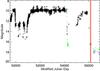 |
Fig. A.1 Light curve of V CrA, based on AAVSO data. The time range is from 01/08/1994 to 29/07/2014. Our observing time is highlighted by the red marker and is clearly during a drop in brightness of the star. The black circles stand for the Vis bandpass, the green points for the V bandpass and the blue points for the B bandpass. |
We observed V CrA during one of these fading events. Indeed, in its spectrum, displayed in Fig. A.2, we are no longer able to see the stellar photospheric absorption lines and we only have an emission spectrum. Because this star is unique in our sample, it is not considered further in this paper.
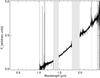 |
Fig. A.2 Spectrum of V CrA, from the UVB to NIR. The UVB and VIS parts of the spectrum are consistent with zero flux. The gray bands mask the regions where telluric absorption is strongest. The areas hatched in black are those that could not be corrected for telluric absorption in a satisfactory way. The area hatched in gray is the merging region between the last two orders of the NIR part. |
Appendix B: Literature properties
Properties of the observed stars (adapted from the literature).
To facilitate future usage of the X-Shooter spectra, we summarize some of the properties of the C-stars observed, as found in the literature or derived therefrom.
In Table B.1, the stars are sorted by RA with horizontal lines facilitating the separation between SMC, LMC and Milky Way sources. The names in Col. 1 are understood by standard interpreters such as those of Centre de Données astronomiques de Strasbourg (CDS). Column 2 provides the reference of the input catalog used in the initial construction of the X-Shooter sample. Our systematic searches of the literature for known stellar properties were made using the generic search through the Vizier catalog database at CDS, as made available via a search link on the Simbad pages of individual objects. Information from other sources was added on a best-effort basis.
Spectral type information was found for only a few of the program stars. The N star T Cae (Alksnis et al. 2001) is labeled C6.4 by Sanford (1944) and C5II by Egret (1980). Alksnis et al. (2001) assign type R0 to the R CrB star V CrA (in its non-obscured phases) and to HD 202851, and type R9 to IRAS 09484-6242. In the LMC, the Mira variable SHV0504353-712622 was of type C7.5 when observed by van Loon et al. (2005).
Columns 3 to 8 of Table B.1 provide pulsation information. The periods and amplitudes in Cols. 3 and 4 are from I band light curves when found, otherwise as specified in Col. 5. Periods followed by a colon are highly uncertain, as the corresponding light curves are very irregular (for most of these stars, a detailed literature search produces half a dozen of very different periods depending on passband, method, and time of observation). The amplitudes given are representative of the peak-to-peak variations over long time spans rather than single-period fits of sine functions (for V CrA, the amplitude given does not include the deep obscuration events). The SR and M variability types in Col. 6 are based on amplitude (as is common practice), not on the shape of the light curve. A comment in Col. 8 summarizes our visual inspection of the available light curves (see Col. 7 for references).
The K magnitude and the (J − K) color taken from 2MASS (Cutri et al. 2003) are listed in Cols. 9 and 10.
The bolometric magnitudes in Col. 11 are apparent when in parentheses, absolute otherwise. For LMC stars, they are taken from Hughes & Wood (1990), who use the bolometric corrections of Wood et al. (1983) and a distance modulus of 18.5. For SMC stars, we list the values of Cioni et al. (2003) when available. They are based on energy distributions from the I band to 12 μm and we assumed a distance modulus of 18.90 to the SMC. We adopted (m − M) = 18.90 for SMC cluster NGC 419 Sloan et al. (in prep.) and (m − M) = 19.06 for NGC 121 (Glatt et al. 2008). For these stars, we use the apparent bolometric magnitudes of Frogel et al. (1990), which are based on the bolometric corrections of Frogel et al. (1980). A more modern compilation of bolometric corrections BC(K) as a function of (J − K) is shown in Nowotny et al. (2013). The spread between authors in that data set amounts to about 0.4 mag. The relations of Wood et al. (1983) and of Frogel et al. (1980) lie near the average of the newer compilation. Representative errors on these are therefore of the order of 0.2 mag.
We have not found distances to the Milky Way stars that we consider reliable, and hence we provide only apparent bolometric magnitudes, based on K, (J − K) and bolometric corrections as above.
Appendix C: Details about the NIR extraction
The 1-dimensional (1D) spectra were extracted from 2D images outside of the pipeline, with a procedure of our own. The underlying idea was to better control the rejection of bad pixels.
The standard acquisition procedure for NIR spectra of point sources is a nodding mode, with observations of the target at two positions (A and B) along the spectrograph slit. By default the pipeline combines the A and B images (flat-fielded and rectified) into a single 2D image in which the central lines contain the sum of the stellar spectra of A and B, minus the sum of the skies. This accumulates the bad pixels of both the A and B positions into the bad pixel mask of the combined spectrum, sometimes leaving very few good pixels to work with. Instead, we extracted A from (A−B) and B from (B−A) and combined them subsequently.
The extraction of a 1D spectrum follows the steps of the optimal extraction of Horne (1986) quite closely, except that no parametric fits are involved in the determination of the 2D stellar illumination profile. For simplicity, we start from rectified, wavelength calibrated 2D images of individual orders of the spectrograph. The inverse variance weighting scheme neglects the correlation between neighbouring pixels that results from the geometrical transformation. Although this is not statistically optimal, it performs better than no variance-weighting and is sufficient for our purpose.
In the following, we will describe the different components of the input 2D spectra (λ, x) as follows:
-
1)
the flux spectrum: D;
-
2)
the variance spectrum: V;
-
3)
the quality spectrum: M. M is set to 1 for good pixels and to 0 for bad pixels.
The first steps of the procedure aim at obtaining a rough first guess for the 1D spectrum.
-
a.
Fit and remove the sky background. The sky background is estimated on one side of the stellar spectrum on the 2D image. At each λ, we calculate the median over x. We then extend this vector over x to create a 2D vector: S. The new image is therefore: (D-S). The variance of the new image is: (VD + VS).
-
b.
Extract the first guess spectrum. The first guess spectrum f1 is obtained by summing the ima-ge along the spatial dimension x. Contrary to Horne (1986), we add the M information, because we find the large values of cosmic ray hits more disturbing than zeros. This choice has no impact on the final result thanks to the smoothing implemented in later steps.
 (C.1)The variance of the standard spectrum V1 is calculated as the sum of the variances along the spatial dimension.
Once the first guess spectrum is extracted, the “optimal” extraction can start. This procedure includes three main steps (c,d,e), and an iteration through all these steps (step f).
-
c.
Construct the spatial profile image. One key component of this procedure is the spatial profile P. A first estimate of this profile is built by dividing each line x of the sky-subtracted image by the current estimate of the 1D stellar spectrum, f. This initial estimate could be noisy and may contain negative values. Therefore, we improve the profile by smoothing in the wavelength direction, assuming that the spatial profile is a slowly varying function of wavelength. We use a median boxcar of 100 Å width. This erases any outlier pixels but keeps track of residual curvature or broadening of the spectral image at the end of orders, which sometimes results from an imperfect rectification. Then, we enforce positivity in our profile, by replacing the negative values by 0, and we normalize at each λ to make sure that the sum over x is unity.
-
d.
Mask the cosmic ray hits. To mask the cosmic ray hits, we evaluate at each wavelength λ the following quantity: (D − S − fP)2/V. If this quantity is higher than a given threshold
 , the pixel with the largest value is rejected. Horne set this threshold to 25, and we set it to 16. Of course, this pixel rejection could be dangerous. Therefore, we reject up to only one pixel per wavelength per iteration, and we update consequently the mask M.
 -
e.
Extract the optimal spectrum. The optimal spectrum is obtained as follows:
![Mathematical equation: \appendix \setcounter{section}{3} \begin{eqnarray} &&f_\lambda = \frac{\sum_{x}MP(D-S)/V}{\sum_{x}MP^2/V}\\ && var[f_\lambda] = \frac{\sum_{x}MP}{\sum_{x}MP^2/V}\cdot \end{eqnarray}](/articles/aa/full_html/2016/05/aa26292-15/aa26292-15-eq94.png)
-
f.
Iterate steps c to e. To complete the procedure, steps c through e are repeated in order to update the spatial profile image P and the bad-pixel mask M, and to create new optimal spectra fλ and var [ fλ ]. This iteration lasts until the set of rejected pixels converges (we allow for a maximum of 3 iterations).
Appendix D: Observed spectra of our sample of carbon stars
Figures D.1 to D.6 show the entire UVB-VIS-NIR spectra for our sample of carbon stars.
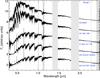 |
Fig. D.1 Spectra of our sample of carbon stars. The gray bands mask the regions where telluric absorption is strongest. The areas hatched in black are those that could not be corrected for telluric absorption in a satisfactory way. The areas hatched in gray are the merging regions between the VIS and NIR spectra and between the last two orders of the NIR part. In some spectra, there is a lack of data at 0.635 μm. The spectra were normalized around 1.7 μm and smoothed by the same factor for display purposes (R ~ 2000). |
Appendix E: Measurements
Tables E.1 and E.2 display the color and index measurements associated with Figs. 14 and 15. Tables E.3, E.4 and E.5 display the color and index measurements for the three comparison samples: Lançon & Wood (2000), Groenewegen et al. (2009) and Rayner et al. (2009).
Color and index measurements for the data from Lançon & Wood (2000) (as in Sect. 7.4).
Color and index measurements for the data from Groenewegen et al. (2009) (as in Sect. 7.4).
Color and index measurements for the data from Rayner et al. (2009) (as in Sect. 7.4).
All Tables
Color and index measurements for the data from Lançon & Wood (2000) (as in Sect. 7.4).
Color and index measurements for the data from Groenewegen et al. (2009) (as in Sect. 7.4).
Color and index measurements for the data from Rayner et al. (2009) (as in Sect. 7.4).
All Figures
|
Fig. 1 Bolometric magnitudes and literature colors of our sample stars. The LMC stars (red triangles) are taken from Hughes & Wood (1990). The SMC stars (blue circles) are derived by Cioni et al. (2003). No reliable distances are known for the MW stars (black squares) of our sample. |
| In the text | |
|
Fig. 2 I-band amplitudes of our sample stars. Symbols are as in Fig. 1. The amplitudes are estimated peak-to-peak variations. The values for LMC stars are taken from Hughes & Wood (1990). For the SMC stars, we estimated amplitudes using OGLE light curves (available through the Vizier service at CDS). For the MW, we estimated amplitudes based on K-band amplitudes by Whitelock et al. (2006); a value of 0.5 was assigned when no data were available. We note that for two MW stars (filled squares) large-amplitude luminosity dips are known to occur occasionally in addition to small-amplitude variations (the R CrB phenomenon). |
| In the text | |
|
Fig. 3 Illustrative spectra in the VIS wavelength range. The red spectrum is a telluric sky model, smoothed to R ~ 10 000. From top to bottom, the stars are 2MASS J01003150-7307237, 2MASS J00571648-7310527, 2MASS J00493262-7317523 and 2MASS J00571214-7307045. Offsets of 0, 2, 4, 6 and 8 flux units have been applied to the C-star spectra and the telluric spectrum for display. |
| In the text | |
|
Fig. 4 Illustrative spectra in the NIR wavelength range. The red spectrum is a telluric sky model, smoothed to R ~ 8000. The stars are the same as in Fig. 3. |
| In the text | |
|
Fig. 5 Representative spectra from our sample of carbon stars. The gray bands mask the regions where telluric absorption is strongest. The areas hatched in black are those that could not be corrected for telluric absorption in a satisfactory way. The areas hatched in gray are the merging regions between the VIS and NIR spectra and between the last two orders of the NIR spectrum. In some spectra, data are missing at 0.635 μm. The spectra have been smoothed for display purposes to R ~ 2000. The colors represent the different groups of carbon stars. Group 1 stars are shown in blue (from top to bottom: HE 1428-1950 and Cl* NGC 121 T V8), Group 2 in red (2MASS J00571214-7307045), Group 3 in orange (from top to bottom: 2MASS J00542265-7301057 and SHV 0502469-692418) and Group 4 in red (from top to bottom: [ABC89] Cir 18 and SHV 0525478-690944). |
| In the text | |
|
Fig. 6 Comparison of our (J − Ks) values with values found in the literature (2MASS values, Cutri et al. 2003). The red line indicates the one-to-one relation. The black points represent the stars with large-amplitude (I amplitude ≥0.8). The bar plotted in the bottom-right corner shows the ±1σ root-mean-square deviation of our photometry with respect to the literature (large-amplitude variables excluded). This is an upper limit of the uncertainties in the flux calibration and any possible residual variability. |
| In the text | |
|
Fig. 7 Zoom into the 12CO(2, 0) feature near 2.3 μm. The red line indicates the region used to calculate the KH86CO1 bandpass, while the blue line corresponds to the KH86c1 bandpass measuring the continuum. This star is 2MASS J00571648-7310527. |
| In the text | |
|
Fig. 8 Zoom into the 12CO(6, 3) line near 1.62 μm. The red lines indicate the features regions, while the blue measure the continuum. The upper panel shows the spectrum of a carbon star, Cl* NGC 121 T V8, in which the 12CO(5, 2) and 12CO(6, 3) bands are visible. The lower panel corresponds to another carbon star, 2MASS J00571214-7307045, in which the CN and C2 lines are more prominent and overlap with the CO lines. The spectra have been normalized at 1.62 μm for display purposes. |
| In the text | |
|
Fig. 9 Zoom into the 13CO(2, 0) line near 2.35 μm. The red line indicates the region used to calculate the KH86CO3 bandpass, while the blue line corresponds to the KH86CO2 bandpass measuring the continuum. This star is SHV 0500412-684054. |
| In the text | |
|
Fig. 10 Zoom into the CN line near 1.1 μm. The red line indicates the region used to calculate the W110 bandpass, while the blue line corresponds to the W108 bandpass measuring the continuum. This star is SHV 0502469-692418. |
| In the text | |
|
Fig. 11 Zoom into the HCN+C2H2 lines around 1.53 μm. The upper panel shows an example of a carbon star, SHV 0502469-692418, in which the HCN+C2H2 feature is visible. The lower panel corresponds to another carbon star, T Cae, in which the feature is missing. The red line indicates the region used to calculate the absorption bandpass, while the blue line corresponds to the continuum bandpass. |
| In the text | |
|
Fig. 12 Zoom into the C2 line around 1.77 μm. The red line indicates the region used to calculate the C2_band bandpass, while the blue line corresponds to the bandpass measuring the continuum. This star is 2MASS J00563906-7304529. |
| In the text | |
|
Fig. 13 The C2 Swan system (top panel) and a zoom into the C2 line around 0.5165 μm. The red line indicates the region used to calculate the C2U_band bandpass, while the blue line corresponds to the C2U_cont bandpass measuring the continuum. This star is HE 1428-1950. |
| In the text | |
|
Fig. 14 Some color–color plots derived from our sample of carbon stars. The red circles stand for carbon stars showing the 1.53 μm feature. For the R filter, we adopt some conservative values. The bars plotted in the bottom-right corners are determined as in Fig. 6. |
| In the text | |
|
Fig. 15 Some indices derived from our sample of carbon stars as a function of (J − Ks). The red circles stand for the carbon stars with the 1.53 μm feature. The filled diamonds represent the averaged values of our indices as a function of the bin number based on (J − Ks), and the bars measure the dispersion within bins. Typical uncertainties on individual measurements are shown in purple. |
| In the text | |
|
Fig. 16 The spread of our sample of carbon stars (circles) in the (J − H)–(H − Ks) color–color plane. The star symbols represent LW2000, the triangles represent Groenewegen et al. (2009) and the squares represent IRTF. Colored symbols stand for those carbon stars with the 1.53 μm feature. |
| In the text | |
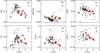 |
Fig. 17 Six of our indices as functions of (J − Ks). Symbols and colors are as in Fig. 16. |
| In the text | |
|
Fig. 18 Two high-resolution, high signal-to-noise ratio C-star spectra for which (J − Ks) ≃ 1.85. Only the top spectrum exhibits the 1.53 μm feature. It also appears smoother in the near-infrared than the bottom one, and it has a peculiar energy distribution. The gray bands mask the regions where telluric absorption is strongest. The areas hatched in black are those that could not be corrected for telluric absorption in a satisfactory way. The areas hatched in gray are the merging regions between the VIS and NIR spectra, and between the last two orders of the NIR part. |
| In the text | |
|
Fig. A.1 Light curve of V CrA, based on AAVSO data. The time range is from 01/08/1994 to 29/07/2014. Our observing time is highlighted by the red marker and is clearly during a drop in brightness of the star. The black circles stand for the Vis bandpass, the green points for the V bandpass and the blue points for the B bandpass. |
| In the text | |
|
Fig. A.2 Spectrum of V CrA, from the UVB to NIR. The UVB and VIS parts of the spectrum are consistent with zero flux. The gray bands mask the regions where telluric absorption is strongest. The areas hatched in black are those that could not be corrected for telluric absorption in a satisfactory way. The area hatched in gray is the merging region between the last two orders of the NIR part. |
| In the text | |
|
Fig. D.1 Spectra of our sample of carbon stars. The gray bands mask the regions where telluric absorption is strongest. The areas hatched in black are those that could not be corrected for telluric absorption in a satisfactory way. The areas hatched in gray are the merging regions between the VIS and NIR spectra and between the last two orders of the NIR part. In some spectra, there is a lack of data at 0.635 μm. The spectra were normalized around 1.7 μm and smoothed by the same factor for display purposes (R ~ 2000). |
| In the text | |
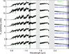 |
Fig. D.2 As for Fig. D.1. |
| In the text | |
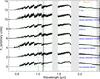 |
Fig. D.3 As for Fig. D.1. |
| In the text | |
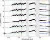 |
Fig. D.4 As for Fig. D.1. |
| In the text | |
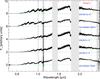 |
Fig. D.5 As for Fig. D.1. |
| In the text | |
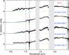 |
Fig. D.6 As for Fig. D.1. |
| In the text | |
Current usage metrics show cumulative count of Article Views (full-text article views including HTML views, PDF and ePub downloads, according to the available data) and Abstracts Views on Vision4Press platform.
Data correspond to usage on the plateform after 2015. The current usage metrics is available 48-96 hours after online publication and is updated daily on week days.
Initial download of the metrics may take a while.