| Issue |
A&A
Volume 587, March 2016
|
|
|---|---|---|
| Article Number | A11 | |
| Number of page(s) | 10 | |
| Section | The Sun | |
| DOI | https://doi.org/10.1051/0004-6361/201525642 | |
| Published online | 11 February 2016 | |
Observations of solar flares with IRIS and SDO
1
Key Laboratory of Dark Matter and Space Science, Purple Mountain
Observatory, CAS,
Nanjing
210008
PR China
e-mail:
lidong@pmo.ac.cn
2
Max-Planck Institute for Solar System Research,
37077
Göttingen,
Germany
3
University of Chinese Academy of Sciences,
Beijing
100049, PR
China
Received: 12 January 2015
Accepted: 16 December 2015
Flare kernels brighten simultaneously in all Solar Dynamics Observatory (SDO) Atmospheric Imaging Assembly (AIA) channels making it difficult to determine their temperature structure. The Interface Region Imaging Spectrograph (IRIS) is able to spectrally resolve Fe xxi emission from cold chromospheric brightenings, so it can be used to infer the amount of Fe xxi emission in the 131 Å AIA channel. We use observations of two small solar flares seen by IRIS and SDO to compare the emission measures (EMs) deduced from the IRIS Fe xxi line and the AIA 131 Å channel to determine the fraction of Fe xxi emission in flare kernels in the 131 Å channel of AIA. Cotemporal and cospatial pseudo-raster AIA images are compared with the IRIS results. We use multi-Gaussian line fitting to separate the blending chromospheric emission so as to derive Fe xxi intensities and Doppler shifts in IRIS spectra. We define loop and kernel regions based on the brightness of the 131 Å and 1600 Å intensities. In the loop regions the Fe xxi EMs are typically 80% of the 131 Å values, and range from 67% to 92%. Much of the scatter is due to small misalignments, but the largest site with low Fe xxi contributions was probably affected by a recent injection of cool plasma into the loop. In flare kernels the contribution of Fe xxi increases from less than 10% at the low-intensity 131 Å sites to 40−80% in the brighter kernels. Here the Fe xxi is superimposed on bright chromospheric emission and the Fe xxi line shows blueshifts, sometimes extending up to the edge of the spectral window, 200 km s-1. The AIA 131 Å emission in flare loops is due to Fe xxi emission with a 10−20% contribution from continuum, Fe xxiii, and cooler background plasma emission. In bright flare kernels up to 52% of the 131 Å is from cooler plasma. The wide range seen in the kernels is caused by significant structure in the kernels, which is seen as sharp gradients in Fe xxi EM at sites of molecular and transition region emission.
Key words: Sun: flares / Sun: UV radiation / line: profiles / techniques: spectroscopic
© ESO, 2016
1. Introduction
The flare impulsive phase is characterized by a sudden increase in chromospheric and hard X-ray emission (Fletcher & Hudson 2001; Fletcher et al. 2011). The emission is concentrated in small bright kernels and along ribbons, coinciding with magnetic field concentrations where rapid chromospheric heating drives hot plasma upward into the corona (Mason et al. 1986; Teriaca et al. 2006; Benz 2008; Ning & Cao 2011). The kernels are thought to be the chromospheric signature of magnetic reconnection in the corona (Qiu et al. 2002; Fletcher et al. 2004; Gan et al. 2008). Spectroscopic observations have revealed high-temperature, high-velocity blueshift and cooler redshift emission (Antonucci et al. 1982; Milligan et al. 2006; Teriaca et al. 2006; Young et al. 2013) compatible with models of chromospheric evaporation.
Observations of the kernels show simultaneous brightening in all Atmospheric Imaging Assembly (AIA) extreme ultraviolet (EUV) channels (Brosius & Holman 2012; Fletcher et al. 2013; Young et al. 2013). The analysis by Brosius & Holman (2012) that compared AIA images with Coronal Diagnostic Spectrometer (CDS) spectra showed that in a small GOES B4.8 flare a significant fraction of the hot channel 94 Å and 131 Å emission could be attributed to the brightening of the transition region and lower coronal lines. On the other hand, Fletcher et al. (2013) attributed all the 131 Å brightening in an M1.0 flare to plasma with temperatures greater than 10 MK. In an M1.1 flare, the Young et al. (2013) analysis of Extreme-Ultraviolet Imaging Spectrometer (EIS) spectra found almost equal emission measures (EMs) across the observed temperature range from 0.1 to 10 MK, but did not discuss the contributions to the AIA channel images.
The main contribution to the 131 Å channel in flares is the Fe xxi 128.75 Å line (O’Dwyer et al. 2010; Milligan & McElroy 2013). The same ion, Fe xxi, produces the strong flare line at 1354.08 Å in the Interface Region Imaging Spectrograph (IRIS) spectra. Therefore, by comparing simultaneous IRIS and AIA observations it may be possible to determine the contribution of Fe xxi to the 131 channel and hence resolve the the question of the cool plasma emission contribution to the 131 channel. Using the same ion, has the advantage that the line ratios are independent of ionization and only weakly dependent on temperature.
The forbidden line of Fe xxi at 1354.08 Å has been used in several spectroscopic studies to investigate hot plasma flow during flares (Doschek et al. 1975; Cheng et al. 1979; Mason et al. 1986; Feldman et al. 2000; Innes 2001; Kliem et al. 2002; Wang et al. 2003). More recently Young et al. (2015) described high spatial and spectral resolution IRIS observations of Fe xxi from hot flare kernels and loops with temperatures of about 10 MK from an X1 class flare. Their results support the chromospheric evaporation model. The Mason et al. (1986) observations indicated that the Fe xxi line is often blended with C i. The higher resolution spectra analyzed by Young et al. (2015) show that the Fe xxi kernel emission may, in addition, be blended with other chromospheric and possibly molecular lines. Molecular hydrogen was identified at the footpoints of X-ray loops with SUMER spectra (Innes 2008). To obtain estimates of the Fe xxi EM, the strength of these chromospheric lines needs to be taken into account. For the analysis in this paper, we investigated a number of flare kernel spectra and developed an algorithm for simultaneously fitting the Fe xxi, blending lines, and continuum.
The EM obtained from the IRIS 1354 Å line was compared with that derived from simultaneous Solar Dynamics Observatory (SDO) AIA 131 Å images to determine the contribution of cooler line emission to the 131 Å channel at the site of flare kernels. We find that the Fe xxi observed by IRIS can account for about 80% of the SDO/AIA 131 Å emission in flare loops and 40−80% of the emission in flare kernels. Assuming that an additional 20% of the Fe xxi is continuum (Milligan & McElroy 2013), we find that up to 52% of the 131 Å channel emission is from cooler plasma in the flare kernels.
2. Observations
The observed active region, AR 11875, produced four C-class flares during the period 16:39 UT on 24 October 2013 and 02:46 UT on 25 October 2013. We obtained high-quality cotemporal and cospatial IRIS and AIA observations for flares at 20:10 and 22:05 UT (Fig. 1). During the early part of the sequence SDO was off-pointing, and during the 21:09 UT flare the IRIS spectra were badly affected by a large number of particle hits. Fig. 2 shows the AIA 131 Å and corresponding slit-jaw (SJ) 1400 Å images of the two flares analyzed. The GOES fluxes of the two flares are shown in Fig. 1. Flare 1 peaked at about 20:10 UT and ended at about 20:22 UT, while flare 2 peaked at about 22:10 UT and stopped at about 22:15 UT.
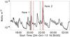 |
Fig. 1 GOES 1.0−8.0 Å flux during the observing period. The two flares analyzed are labeled. Red lines are drawn at the times of the peak flux, while the dashed lines show the start and end times of the of IRIS raster 6 (between 20:02 UT and 20:35 UT) and raster 9 (from 21:43 UT to 22:16 UT). |
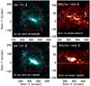 |
Fig. 2 Left: AIA 131 Å images of the active region at the times of the two flares. The red boxes are the positions of the IRIS SJ images. Right: IRIS SJ 1400 Å images of the two flares analyzed. The position of the spectrometer slit at the start of the flare is seen as a white dashed horizontal line. The purple +’s indicate the re-spike pixels in the AIA 131 Å images with the code “aia_ respike”. |
2.1. AIA observations
In this analysis, AIA images (Lemen et al. 2012) from the 131 and 1600 Å channels are used for comparison with the IRIS data. The AIA level 1.0 data were downloaded and processed to level 1.5 using the standard solarsoft (SSW) routines. Then using the code drot_map.pro in SSW, the active region with a field of view of 420′′× 420′′ are selected from the AIA full disk images (see Fig. 2). The images from different AIA filters have alignment uncertainties of about 1−2 pixels (e.g., Young et al. 2013). Therefore the AIA 131 Å images are slightly shifted (i.e., 0.5−2 pixels) with respect to the 1600 Å images because we obtained the best alignment of the 1600 Å with the IRIS 1400 Å and the 131 Å with the IRIS Fe xxi.
The downloaded AIA data are already de-spiked, which often removes flare kernel emission and these can be put back with the aia_respike routine (see Young et al. 2013). In our study, we compared the “re-spike” data and the level 1 data at 131 Å as shown with the purple plus signs in Fig. 2. This shows that the re-spiked pixels are far away from the IRIS slit position, and they are not within the regions of our study. This was the case for all other 131 Å images. Furthermore, during big flares the AIA 131 Å channel is often saturated. The two flares in this paper are quite small and very few pixels in the 131 Å channel were saturated. Fortunately, those saturated pixels are far away from the IRIS raster slit. In other words, neither the de-spiking nor the saturated pixels are a problem in our study.
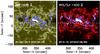 |
Fig. 3 Coalignment of the SDO and IRIS images. Left: the AIA image at 1600 Å. Right: the SJ image at 1400 Å. The white dashed line is the IRIS slit position, and the blue contours are the SJ intensity at the level of 800 DN. |
2.2. IRIS observations
IRIS is a NASA Small Explorer Mission launched in June 2013, and its main science is an investigation of the dynamics of the Sun’s chromosphere and transition region (McIntosh et al. 2013). As described in detail by De Pontieu et al. (2014), IRIS is a high-resolution spectrograph and slit-jaw (SJ) camera that obtains spatial resolution of 0.33−0.4 arcsec and spectral resolution of ~26 mÅ (or ~52 mÅ in second order). There are three IRIS wavelength bands: (i) 1332−1358 Å, which includes the strong C ii doublet, Fe xxi, and a number of strong C i lines; (ii) 1389−1406 Å, which includes the Si iv doublet and density sensitive O iv lines; and (iii) 2782−2834 Å, which includes Mg ii h and k lines. Here we analyze lines in the 1332−1358 Å range. IRIS also obtains SJ images centered at 1330, 1400, 2796, and 2832 Å.
The observations described here were designed with the aim of capturing the structure and spectra of flares by making rapid rasters across a flaring active region for as long a period as telemetry constraints allowed. The IRIS rasters were obtained by taking 64 1.01′′ steps across a region 174′′× 63′′ with the roll angle 90° (i.e., the slit was oriented E-W). Simultaneous SJ images at 1400 Å with a field of view 174′′× 166′′ and cadence 32 s were also obtained and used mainly for coalignment with 1600 Å AIA images. Because continuum emission from the temperature minimum is dominant in many of the bright features seen in both sets of images, coalignment is possible to within the AIA pixel size, 0.6′′ (Fig. 3).
The step cadence was 31.6 s and the exposure time 30 s, thus the raster cadence was 33 m 42 s. Eighteen rasters were obtained in the roughly ten-hour period. The pixel size along the slit was at the highest resolution 0.167′′, but four times spectral binning and a restricted number of spectral windows were obtained to save telemetry. In this case we used the flare list of lines, which consisted of the C ii, 1343, Fe xii, O i, and Si iv far-ultraviolet (FUV) windows. Here we only discuss spectra from windows in the short wavelength FUV band. The spectral resolution was 4*12.72 mÅ/pixel, equivalent to 10.88 km s-1/pixel.
IRIS level 2 data were downloaded. These data were calibrated and corrected for image distortions. Several of the images were badly affected by particle hits and hot or dead pixels, which were removed using a despiking routine that detected persistent hot/dead pixels and sudden changes in intensity since they can seriously distort the line fitting results. Care is taken to ensure that only isolated bright pixels or small pixel groups are removed, and to leave intensity changes due to sudden line broadening. Figure 4 shows the effect of de-spiking. In addition, small spectral shifts caused by thermal drifts and the spacecraft orbital velocity were corrected with the routine iris_orbitvar_corr_12.pro (McIntosh et al. 2013; Tian et al. 2014; Cheng et al. 2015) in the SSW package.
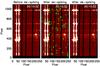 |
Fig. 4 IRIS raster images before (left) and after de-spiking (right). The middle panel is an image after de-spiking with the bad pixels marked with green +’s. |
2.3. Flare ribbon spectra
The ribbons are characterized by many narrow, bright emission lines. The Fe xxi emission blends with both known and unknown lines from neutral and singly ionized species, as well as molecular fluorescence lines. To determine the Fe xxi intensity we need to extract the blending chromospheric emission. We have identified the main blending lines by looking at kernel spectra from other IRIS datasets at higher spectral resolution, as well as many spectra in this dataset to find out which other observed lines behave similarly to the chromospheric lines in the Fe xxi window. An example of a flare footpoint spectrum taken with this sequence is shown in Fig. 5. For comparison, the chromospheric lines seen during a C1.5 flare from AR11861 (−133′′, −285′′) at 00:46 UT on 12 October 2013, taken with the full spectra resolution, are shown in Fig. 6.
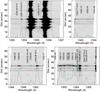 |
Fig. 5 Flare footpoint spectra taken on 24 October 2013. The overplotted line spectra are the average across the small bright region marked by a red line on the left-hand side of each image. The main lines are labeled and indicated by light blue vertical ticks just above the line spectra. |
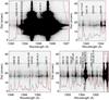 |
Fig. 6 Flare footpoint spectra taken on 12 October 2013 at full resolution. The overplotted line spectra are the average across the small bright region marked by a red line on the left-hand side of each image and, in red, the same spectra binned by a factor of 4, which is the resolution used on 24 October 2013. |
The main chromospheric lines in the O i window, apart from the C i 1354.29 Å line, are the Fe ii lines at 1353.02, 1354.01, and 1354.76 Å; the Si ii lines at 1352.74 and 1353.72 Å; and the unidentified lines at 1353.32 and 1353.39 Å. Actually, other papers (e.g., Graham & Cauzzi 2015; Li et al. 2015; Tian et al. 2015) have attempted multi-Gaussian fits to the Fe xxi line from IRIS spectral observations. In this paper, to obtain the Fe xxi intensities, we fixed or constrained the positions and widths of these lines and set their intensities to have a specified ratio to well-resolved lines from similar species. In total we fit 17 Gaussian lines superimposed on a linear background fitted across the wavelength region (i.e., 1333.01−1355.55 Å) covered by the four IRIS spectral windows. Table 1 lists the lines used in the fitting procedure. Lines with fixed positions are indicated by a superscript “1”. The two Si ii lines, indicated with a superscript “2”, are constrained to match the shift of the unblended Si ii at 1350.06 Å. The widths are fixed or constrained as given in column 4. For example, the Si ii 1353.72 line has a maximum width of 260 mÅ, while the line width of Fe ii 1353.02 is fixed at 41 mÅ. The peak intensities of the blending lines are forced to be in a fixed ratio (Col. 6) with the lines that they are tied to (Col. 5). For example, the peak intensity of the blending line Si ii 1353.72 is tied to the emission line Si ii 1350.06 in the Fe xii window, and the intensity ratio is 0.49. The positions and intensity ratios of the lines were determined by fitting Gaussians to all the narrow (identified and unidentified) lines in 17 spectra in the dataset with bright molecular and chromospheric lines but no Fe xxi emission. For each line, the median position from the 17 spectral fits was taken as the line’s fixed position. Then for each narrow line blending with the Fe xxi, we calculated its intensity ratio with respect to all unblended narrow lines. We used the variation in the intensity ratios to identify which line each blended lines should be tied to, and the median of the ratio was used to determine the strength of the blended line from the intensity of its tied line. The lines used in the final fitting procedure to obtain the Fe xxi intensities are marked and the regions of background are indicated by the red dashed lines in Fig. 7. At most positions the fits appear to be successful.
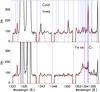 |
Fig. 7 Spectra (black) and multi-Gaussian fits (red). The blue dashed lines mark the positions of cold lines, the blue solid line marks the C i line, while the purple line marks the Fe xxi line. |
Seventeen emission lines from the four IRIS spectral windows used in the multi-Gaussian fit.
3. Emission measures of Fe xxi
The observed intensity is given by 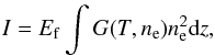 (1)where \begin{lxirformule}$n_{\rm e}$\end{lxirformule} is the electron density, T is electron temperature, z is the line-of-sight coordinate, G(T,ne) is the contribution function of the line including the atomic abundance, and Ef is the instrument effective area or response function. In the equation above the units of I depend on the units of the Ef. As discussed below, IRIS is a spectrometer and the intensities are given in DN s-1; AIA is an imager and the intensity unit is DN px-1 s-1. To convert intensity to emission measure, we need to divide by the respective response functions in the appropriate units. Since the contribution functions of the IRIS and AIA Fe xxi lines are sharply peaked in temperature and are formed over the same heights, the contribution functions can be removed from the integral. The emission measure in the Fe xxi plasma can then be calculated from
 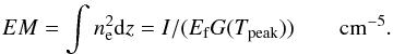 (2)
(2)
The temperature response, EfG(Tpeak), for the AIA 131 Å channel and the IRIS 1354 Å line are shown in Fig. 9. The AIA function has been computed with the procedure aia_get_response.pro with the calibration appropriate to the time of the observation at the default pressure in CHANTI of 1015 cm-3 K (Boerner et al. 2012). The keyword “chiantifix” is also set to account for emission that is not included in the CHIANTI database (Testa et al. 2012; DeRosa & Slater 2013). The response of AIA to high- and low-temperature flare emission is believed to be accurate to 25% with these empirical corrections (Boerner et al. 2012). There are two peaks, one due to Fe viii formed around 6 × 10⁵ K and the other due to Fe xxi formed around 107 K. The main variation in the contribution function around 10 MK comes from the dependence of ionization on temperature. The IRIS Fe xxi line is a fine structure transition within the ground state so its excitation rate is independent of temperature, but at high densities (ne> 1012 cm-3) it suffers from collisional de-excitation. Figure 8 shows the variation of the 128.75/1354.08 line ratio, computed with CHIANTI (Landi et al. 2013), as a function of density for three temperatures close to the peak of the contribution function. The temperature variation at low densities varies by less than 7% over the range shown. Only at temperatures below 4 MK is there a significant temperature dependence on the ratio. We assumed the low-density limit and temperature 11 MK and computed the Fe xxi response function as the line emissivity divided by the radiometric conversion coefficient, 2960 (De Pontieu et al. 2014), and the spectral scale (0.0128 Å). Again, the electron pressure was set to 1015 cm-3 K. The radiometric conversion for the IRIS spectra is based on the International Ultraviolet Explorer (IUE) spectral radiances, which has an uncertainty of 10−15% (one σ). Both the AIA and IRIS emissivities are computed at the same pressure, elemental abundance, and ionization. In the analysis of the Fe xxi contribution to the 131 channel, we assume that the ratio of the intensities is constant.
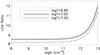 |
Fig. 8 Variation of the Fe xxi 128.75/1354.08 ratio as a function of density, which is from CHIANTI V. 7.1.3 (Landi et al. 2013). |
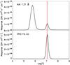 |
Fig. 9 Temperature response of the AIA 131 Å channel (top) and the IRIS Fe xxi 1354 Å line (bottom). The red lines are drawn at the peak of the response curves, 11 MK. |
Fe xxi emission measure maps can be obtained by dividing the observed intensities (DN s-1) by the value of the peak response, at 11 MK, of the respective functions. To compare the IRIS and AIA results pixel-by-pixel pseudo rasters were constructed from a series of AIA images by selecting the overlapping AIA pixels from the closest in time AIA image for each IRIS raster position. Along the slit, each AIA pixel (0.6′′) is about 3.6 IRIS pixels (0.167′′). We map the IRIS pixels onto the AIA grid and average the IRIS intensity in each AIA pixel. The IRIS raster step size (1.01′′) is larger than the AIA pixels so in the raster direction the single overlapping IRIS pixel is used. Thus, the IRIS data have been averaged across ~3.6 pixels in the slit direction so that the IRIS data are re-binned to the scale of the AIA data. In the raster direction, the AIA pseudo rasters are taken from the closest time AIA data.
4. Results
4.1. Images and spectra
There were two well-observed solar flares, as shown in Fig. 2. The IRIS spectra of the two flares were fitted, as described, with 17 Gaussians superimposed on a linear background. The primary lines of interest are the Fe xxi 1354.08 Å and, to a lesser extent, C i 1354.29 Å. Figs. 10 and 12 compare IRIS Fe xxi and C i intensity images with AIA 131 and 1600 Å pseudo-rasters of flare 1 and flare 2. The regions of enhanced C i identify the flare kernels. The Fe xxi Doppler velocity is shown in the bottom left panel. From the velocity images we can see that the Fe xxi is blueshifted near the start of the flare near the flare kernels. As shown, bright C i overlaps very well with the bright 1600 Å emission. The highest velocity measured is about 200 km s-1.
To look closely at the emission from the kernels, we extracted spectra from almost neighboring positions along the slit. The points are shown by plus signs (“+”) in Figs. 10 and 12. In Figs. 11 (flare 1) and 13 (flare 2), we show spectral images and spectra from the first raster step with Fe xxi kernel emission, as well as spectra taken at the same positions from the earlier and later raster steps. The resultant fits appear to be very good. In both flares, the Fe xxi appears as a broad line below the narrow chromospheric lines. The main sources of uncertainty in the Fe xxi intensity come from the background fit, the edge of the spectral window, and the possibly non-Gaussian Fe xxi profile. The background is fitted across all spectral windows and so is fairly well constrained, and the window edge only affects the few positions where Fe xxi is blueshifted by more than 150 km s-1.
As well as assessing the fits by eye we also computed the χ2 for the spectral region around the Fe xxi line. The values were generally less than one. At one or two positions, the χ2 was large (>10). Here the peak of the C i line could not be fit correctly by a Gaussian possibly due to optical depth effects. Occasionally individual narrow lines blending with Fe xxi caused χ2 of about 3 at the position of the Fe xxi line. Since they were much narrower than the Fe xxi they did not affect the Fe xxi intensity.
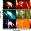 |
Fig. 10 Images of the first flare: (top) IRIS Fe xxi 1354.08 Å and C i 1354.29 Å intensity; (middle) AIA 131 Å and 1600 Å pseudo-raster intensity; (bottom) IRIS Fe xxi Doppler velocity and continuum intensity. The green rectangle marked with +’s indicates the region and sites of the spectra shown in Fig. 11. The arrow indicates the time direction; the duration of these images is 11 m 4 s. The duration of the raster is indicated in Fig. 1. |
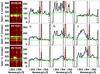 |
Fig. 11 Flare-kernel spectra from the region inside the green rectangle in Fig. 10: (left-middle) the spectrogram of the region marked with a green rectangle in Fig. 10, with before (left-top) and after (left-bottom) spectrograms. The right panels show the spectra (solid) and their fits (dashed) at the positions indicated by the green lines in the left panel. The vertical solid lines give the rest wavelength of Fe xxi and the vertical dashed-dot lines give the rest wavelength of C i line. The green solid line is the background, the blue dashed line is the background + Fe xxi line fit, and the red dashed line is the background + C i line fit. |
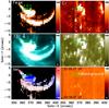 |
Fig. 12 Images of the second flare. (top) IRIS Fe xxi 1354.08 Å and C i 1354.29 Å intensity; (middle) AIA 131 Å and 1600 Å pseudo-raster intensity; (bottom) IRIS Fe xxi Doppler velocity and continuum intensity. The green rectangle marked with +’s indicates the region and sites of the spectra shown in Fig. 13. The arrow indicates the time direction; the duration of these images is 11 m 4 s. The duration of the raster is indicated in Fig. 1. |
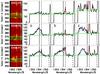 |
Fig. 13 Flare-kernel spectra from the region inside the green rectangle in Fig. 12: (left-middle) the spectrogram at the time of the rectangle region in Fig. 12, with before (top) and after (bottom) spectrograms. Right: spectra and their fits (dashed lines) at the positions marked by the green lines in the left panel. The vertical solid lines indicate the rest wavelength of Fe xxi, and the vertical dash-dotted lines indicate the rest wavelength of C i. The green solid line is the background, the blue dashed line is the background + Fe xxi line fit, and the red dashed line is the background + C i line fit. |
4.2. Emission measures of AIA 131 Å and Fe xxi
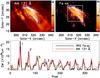 |
Fig. 14 Upper: emission measures computed from AIA 131 Å and IRIS Fe xxi at 11 MK for the first flare. The white box is the region over which we compare EMs in the panels below. Bottom: pixel-by-pixel and row-by-row EMs across the white box region, starting from the upper left. The black line is the Fe xxi EM, and the red line is the 131 Å EM. The +’s indicate those pixels where the Fe xxi emission is higher, and the ×’s mark the selected pixels shown in Fig. 15. |
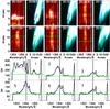 |
Fig. 15 Selected IRIS spectra and AIA intensities for the first flare. The vertical dashed lines in the AIA images are the positions of the IRIS slits. The numbers on the IRIS images show the positions of the selected points in Fig. 14. The +’s and ×’s in the AIA images indicate the positions of these points in the AIA images. Underneath are the IRIS spectra (solid black line) and their fits (black dashed line) for the selected positions. The green solid line is the background, the blue dashed line is background + Fe xxi line, while the vertical line is the rest wavelengths of the Fe xxi line. |
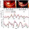 |
Fig. 16 Emission measures from AIA 131 Å and IRIS Fe xxi at 11 MK for the second flare. The two white boxes are the selected regions (R1 and R2). In the lower panels, the black line is the Fe xxi EM, and the red line is the 131 Å EM. The +’s mark pixels where the Fe xxi EM is higher , and the ×’s mark selected pixels, shown in Fig. 17 with higher 131 EM. |
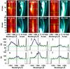 |
Fig. 17 Selected IRIS spectra and AIA intensities for the second flare. The vertical lines in the AIA images mark the positions of the IRIS slits. The numbers on the IRIS images show the positions of the selected points in Fig. 16. The +’s and ×’s in the AIA images mark the positions of these points in the AIA images. Underneath are the IRIS spectra (solid black line) and their fits (black dashed line). The green solid line is the background, the blue dashed line is background + Fe xxi line, while the vertical line is the rest wavelength of Fe xxi line. |
From Eq. (2) we can estimate the EMs of the AIA 131 and IRIS Fe xxi emitting plasma. Figure 14 shows the result for the first flare. The upper panels are the images of the EMs with contours of the IRIS Fe xxi EM. The images of the EMs have a logarithmic scaling, and show good qualitative agreement. The lower panel shows the comparison of the two EMs. To look closer at the overlap, we selected the smaller region (surrounded by the white box) and perform a row-by-row comparison of the EMs of AIA 131 and Fe xxi in the panel underneath. The structures match closely. The AIA 131 EMs are more diffuse and greater than Fe xxi EMs except around positions 1 and 2. As a check on the Gaussian line fit, we show the spectra and fits at the numbered positions in Fig. 15. All fits appear to be very good and there is no special feature of position 1 or 2 to indicate why the computed Fe xxi EMs are higher than the 131 EMs.
We checked whether the higher EMs were due to a temporal mismatch between IRIS and AIA. AIA produced two 131 Å exposures during each IRIS exposure (30 s) so we compared with both of the overlapping AIA images separately for these and all other points and found only very small differences. We therefore conclude that it is not a temporal effect. It could be an effect of the two different spatial resolutions. The IRIS slit only samples about half of the AIA pixel so if the features are very concentrated, the filling factor may be less in AIA than in IRIS. This would result in a lower AIA than IRIS EM.
Similar plots for the second flare are shown in Figs. 16 and 17. The region of bright Fe xxi is slightly larger in the second flare so we split the region into two, labeled “R1” and “R2” in Fig. 16. Again, selected spectra are shown (see Fig. 17). The overall behavior is similar to that seen in the first flare: the 131 EMs are higher and more diffuse than the Fe xxi EMs. At position 4, the IRIS EM is larger than the 131. As shown in Fig. 17, this point is also on the edge of a loop, so it may again be indicating a slight coalignment mismatch. We also note that at position 2, which is near the peak in the 131 emission, the IRIS EM is only about two-thirds of the 131 EM. As seen in Fig. 17, the IRIS spectra at this position show a blueshift of about 0.5 Å or 100 km s-1. Blueshifts in flares are usually linked to chromospheric evaporation, which implies that a range of ionization states can be expected, including Fe viii at this position. Further support for this conclusion comes from the time evolution that showed brightening at this site in all AIA channels at the time of the IRIS observations.
To obtain quantitative values we separate the two flare regions into loops and kernels and compare the IRIS-to-AIA EM ratios as a function of Fe xxi or 131 intensity. We plot the ratio of 131 EM to the sum of 131 and Fe xxi EMs to avoid going off the scale when the Fe xxi EM is very low. Thus, when the 131 EM is due to Fe xxi alone, the ratio is 0.5. A contribution to the 131 EM from cooler lines, continuum, or Fe xxiii would produce a value closer to one, and where there is no Fe xxi contribution, the value is one. The results for the two flares are shown in Figs. 18 and 19. The selection of loop and kernel regions is based on the AIA 131 and 1600 Å intensities. Pixels with 131 Å intensities greater than twice 131 Å average and 1600 Å intensities less than twice 1600 Å average are selected as loops and those with 1600 Å intensities greater than twice 1600 Å average are selected as kernels.
For loops the average value of the ratio is 0.54 in flare 1 and 0.55 in flare 2. The ratio is almost constant across the intensity range. This implies that typically about 80−85% of the 131 Å loop emission is from Fe xxi which is consistent with Milligan & McElroy (2013) who estimate a 20% continuum contribution to the 131 Å channel during flares.
For flare 1, the ratio ranges from 0.2 to 0.6. The low values can be attributed to alignment or filling factor issues. For example the single point in the highest intensity bin in flare 1 is from a bright point on the edge of the kernels. The two points in the next highest intensity bin with a ratio below 0.5 are also from the edge of the kernel region. The other points with ratios less than 0.5 are from the bright western edge of the 131 Å region where both the Fe xxi and 131 Å emission rapidly decreases. The higher ratio values are mostly from the lowest intensity bin on the edge of the loop regions. These may be due to cooler material on the edge of the loop or background 131 Å emission. Therefore the typical loop value in flare 1 is the mean of the low-intensity bins, 0.55 or 81% Fe xxi.
The flare 2 loops have more scatter in their ratio. In the highest intensity bin, there are four points with a ratio around 0.6 (67% Fe xxi). These are from the bright region at the center of R1. As mentioned, these points have blueshifted Fe xxi and at the same time are brightened in all AIA channels, suggesting that it is a site of chromospheric evaporation, not a typical loop. The scatter in the low-intensity bins is mostly caused by coalignment issues in the R2 region as can be seen in Fig. 16. The last row, around position 7, produced many of the high ratio points. These points are along the edge of the loop and – like the edges of the loops in flare 1 – may be due to cooler material on the edge of the loop or background 131 Å emission. In flare 2, the average value 0.55 (81%) Fe xxi is typical for the 131 Å loops.
The ratio in the kernels covers the full range from 0−100% Fe xxi. We have plotted the ratio as a function of both Fe xxi and 131 intensity. As the intensities increase the contribution of Fe xxi to the 131 Å channel increases up to the value seen in the loops. In flare 1, as noted above and shown in Fig. 18, the Fe xxi EM is greater than the 131 EM in the brightest pixels. We attribute this to imperfect coalignment or different filling factors for the two instruments, so the ratio in the two highest intensity bins of flare 1 are not included in our final conclusions. Below a 131 Å intensity of 600 DN s-1, a significant fraction of pixels have no Fe xxi emission. Thus, there is structure within the kernels on the scale of the AIA pixel size, 0.6′′. If the 131 pixels in the middle of the intensity range are considered, the ratio is between 0.55 and 0.75 (see Figs. 18 and 19), which implies that the 131 kernel EM is between 20−60% greater than the Fe xxi EM. This broad range again implies a high-resolution structure in the kernels not seen in the 131 Å images. If the continuum emission is about 20% of the Fe xxi as found by Milligan & McElroy (2013), then our result implies that from zero to 52% of the flare kernel 131 Å emission is due to cooler plasma emission.
These results assume that both instruments are well calibrated and the data are coaligned. The fact that we obtain a consistent value of 80% Fe xxi contribution to the 131 channel in the loops suggests that the calibration is good. A 20% error in the intercalibration would lead to a 10% change in the Fe xxi contribution.
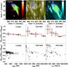 |
Fig. 18 Quantitative analysis of the Fe xxi and 131 Å EMs for flare 1. The top row from left to right shows Fe xxi, 1600 Å, and 131 Å intensity. The middle panels show the mean and median (red line) ratios EM(131)/(EM(131)+EM(Fe xxi)) vs. Fe xxi intensity in loops (bin = 400 DN) and kernels (bin = 400 DN), and on the right the ratio EM(131)/(EM(131)+EM(Fe xxi)) vs. intensity of 131 Å (bin = 400 DN s-1). The bottom panels show the same ratios vs. intensity but as scatter plots. In the loops the mean, standard deviation, and median ratios are 0.54 ± 0.07 and0.55. |
5. Conclusions and discussion
Using the high-resolution IRIS spectral data together with the SDO data, we study two solar flares in AR 11875 that occurred on 24 October 2013. We obtain the intensity of Fe xxi from IRIS data and compare it with AIA data at 131 Å. Coalignment to an accuracy of one AIA pixel (0.6′′) is achieved by coaligning the IRIS C i to AIA 1600 Å (see Fig. 3) and the IRIS Fe xxi to AIA 131 Å images. Fe xxi is a hot, broad line, which in flare kernels is blended with many cold lines. Previous studies (Doschek et al. 1975; Cheng et al. 1979; Mason et al. 1986) at lower resolution only consider blending of Fe xxi with the C i line. However, as IRIS reveals, there are several additional cold chromospheric lines blending with the Fe xxi (see Fig. 7). After studying other IRIS flare kernel spectra, we were able to identify lines in different parts of the IRIS spectrum that can be used to constrain the intensity, widths, and positions of the blending cold lines (see Table 1). Using 17 Gaussian lines and a linear continuum we are able to fit the spectra and obtain reliable Fe xxi intensities at all positions.
The spectra show regions at the onset of the flares where of Fe xxi is coincident with cold-line emission (see Figs. 10 and 12). We have carefully checked the fits to make sure that the procedure has worked at these positions (see Figs. 11 and 13). In these regions, the Fe xxi line shows high blueshifts up to 200 km s-1, which is the edge of the spectral window. This velocity is also consistent with other hot spectral lines seen in flares, such as Fe XIX (Czaykowska et al. 2001; Teriaca et al. 2003; Brosius & Phillips 2004), Fe XXIII, and Fe XXIV (Milligan & Dennis 2009). In our study, the EMs have a magnitude of about 1028 cm-5, although some pixels can reach 1029 cm-5 (see Figs. 14 and 16), which also agrees with others (Graham et al. 2013; Fletcher et al. 2013).
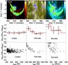 |
Fig. 19 Quantitative analysis of the Fe xxi and 131 EMs for flare 2. The top row from left to right shows Fe xxi, 1600 Å, and 131 Å intensity. The middle panels show the mean and median (red line) ratios EM(131)/(EM(131)+EM(Fe xxi)) vs. Fe xxi intensity in loops (bin = 300 DN) and kernels (bin = 300 DN), and on the right the ratio EM(131)/(EM(131)+EM(Fe xxi)) vs. intensity of 131 Å (bin = 300 DN s-1). The bottom panels show the same ratios vs. intensity but as scatter plots. In the loops the mean, standard deviation, and median ratios are 0.55 ± 0.06 and 0.54. |
It is well known that the 131 Å channel in AIA has contributions from the Fe xxi and the Fe viii line. Brosius & Holman (2012) list a number of other transition region lines that may also be present. We compare the EMs of AIA 131 Å and the IRIS Fe xxi line pixel-by-pixel, assuming all emission is from hot plasma. For loop regions the AIA 131 Å EMs are about 20% greater than the Fe xxi EMs (see Figs. 18 and 19). This is consistent with the analysis of Milligan & McElroy (2013) that 20% of the 131 Å channel emission is due to continuum in flares. We also identified a loop region with about 33% greater 131 than Fe xxi EM. Since, this region simultaneously brightened in all AIA channels and was associated with Fe xxi blueshifts, we attribute the lower-than-average Fe xxi to additional Fe viii due to a recent injection of cool plasma into the loop. In the brighter 131 flare kernels (>600 DN s-1), the 131 EM is about 20−60% more than the IRIS Fe xxi suggesting that there is a contribution of up to 52% from cool plasma emission (Brosius & Holman 2012).
A small-scale kernel structure results in a broad range of 131/Fe xxi EM ratios and sharp gradients in IRIS Fe xxi emission at sites of molecular and transition region emission. At the start of the flare, consecutive raster steps showed a large increase in Fe xxi across the kernels indicating that the kernel structure is both temporal and spatial. Future work will focus on the analysis of flares obtained at higher spectral resolution with broader wavelength windows and higher temporal cadence to resolve the temporal/spatial ambiguities.
Acknowledgments
The authors would like to thank the anonymous referee for valuable comments that improved the manuscript. IRIS is a NASA small explorer mission developed and operated by LMSAL with mission operations executed at NASA Ames Research center and major contributions to down-link communications funded by the Norwegian Space Center (NSC, Norway) through an ESA PRODEX contract. We are indebted to the IRIS and SDO teams for providing the high-resolution data. We would also like to thank the people at MPS, in particular Professor Hardi Peter, Doctors Li, Leping, Chen, Feng and Guo, Lijia.
References
- Antonucci, E., Gabriel, A. H., Acton, L. W., et al. 1982, Sol. Phys., 78, 107 [NASA ADS] [CrossRef] [Google Scholar]
- Benz, A. O. 2008, Liv. Rev. Sol. Phys., 5, 1 [Google Scholar]
- Boerner, P., Edwards, C., Lemen, J., et al. 2012, Sol. Phys., 275, 41 [NASA ADS] [CrossRef] [Google Scholar]
- Brosius, J. W., & Holman, G. D. 2012, A&A, 540, A24 [NASA ADS] [CrossRef] [EDP Sciences] [Google Scholar]
- Brosius, J. W., & Phillips, K. J. H. 2004, ApJ, 613, 580 [NASA ADS] [CrossRef] [Google Scholar]
- Cheng, C.-C., Feldman, U., & Doschek, G. A. 1979, ApJ, 233, 736 [NASA ADS] [CrossRef] [Google Scholar]
- Cheng, X., Ding, M. D., & Fang, C. 2015, ApJ, 804, 82 [NASA ADS] [CrossRef] [Google Scholar]
- Czaykowska, A., Alexander, D., & De Pontieu, B. 2001, ApJ, 552, 849 [NASA ADS] [CrossRef] [Google Scholar]
- De Pontieu, B., Title, A. M., Lemen, J. R., et al. 2014, Sol. Phys., 289, 2733 [NASA ADS] [CrossRef] [Google Scholar]
- DeRosa, M., & Slater, G. 2013, Guide to SDO Data Analysis edited on February 19, 2013 [Google Scholar]
- Doschek, G. A., Dere, K. P., Sandlin, G. D., et al. 1975, ApJ, 196, L83 [NASA ADS] [CrossRef] [Google Scholar]
- Feldman, U., Curdt, W., Landi, E., & Wilhelm, K. 2000, ApJ, 544, 508 [NASA ADS] [CrossRef] [Google Scholar]
- Fletcher, L., & Hudson, H. 2001, Sol. Phys., 204, 69 [NASA ADS] [CrossRef] [Google Scholar]
- Fletcher, L., Pollock, J. A., & Potts, H. E. 2004, Sol. Phys., 222, 279 [NASA ADS] [CrossRef] [Google Scholar]
- Fletcher, L., Dennis, B. R., Hudson, H. S., et al. 2011, Space Sci. Rev., 159, 19 [NASA ADS] [CrossRef] [Google Scholar]
- Fletcher, L., Hannah, I. G., Hudson, H. S., & Innes, D. E. 2013, ApJ, 771, 104 [NASA ADS] [CrossRef] [Google Scholar]
- Gan, W. Q., Li, Y. P., & Miroshnichenko, L. I. 2008, Adv. Space Res., 41, 908 [NASA ADS] [CrossRef] [Google Scholar]
- Graham, D. R., & Cauzzi, G. 2015, ApJ, 807, L22 [NASA ADS] [CrossRef] [Google Scholar]
- Graham, D. R., Hannah, I. G., Fletcher, L., & Milligan, R. O. 2013, ApJ, 767, 83 [NASA ADS] [CrossRef] [Google Scholar]
- Innes, D. E. 2001, A&A, 378, 1067 [NASA ADS] [CrossRef] [EDP Sciences] [Google Scholar]
- Innes, D. E. 2008, A&A, 481, L41 [NASA ADS] [CrossRef] [EDP Sciences] [Google Scholar]
- Kliem, B., Dammasch, I. E., Curdt, W., & Wilhelm, K. 2002, ApJ, 568, L61 [NASA ADS] [CrossRef] [Google Scholar]
- Landi, E., Young, P. R., Dere, K. P., Del Zanna, G., & Mason, H. E. 2013, ApJ, 763, 86 [NASA ADS] [CrossRef] [Google Scholar]
- Lemen, J. R., Title, A. M., Akin, D. J., et al. 2012, Sol. Phys., 275, 17 [NASA ADS] [CrossRef] [Google Scholar]
- Li, D., Ning, Z. J., & Zhang, Q. M. 2015, ApJ, 807, 72 [NASA ADS] [CrossRef] [Google Scholar]
- Mason, H. E., Shine, R. A., Gurman, J. B., & Harrison, R. A. 1986, ApJ, 309, 435 [NASA ADS] [CrossRef] [Google Scholar]
- McIntosh, S. W., De Pontieu, B., Hansteen, V., & Boerner, P. 2013, A User’s Guide To IRIS Data Retrieval, Reduction and Analysis, October, 30 [Google Scholar]
- Milligan, R. O., & Dennis, B. R. 2009, ApJ, 699, 968 [NASA ADS] [CrossRef] [Google Scholar]
- Milligan, R. O., & McElroy, S. A. 2013, ApJ, 777, 12 [NASA ADS] [CrossRef] [Google Scholar]
- Milligan, R. O., Gallagher, P. T., Mathioudakis, M., et al. 2006, ApJ, 638, L117 [NASA ADS] [CrossRef] [Google Scholar]
- Ning, Z., & Cao, W. 2011, Sol. Phys., 269, 283 [NASA ADS] [CrossRef] [Google Scholar]
- O’Dwyer, B., Del Zanna, G., Mason, H. E., Weber, M. A., & Tripathi, D. 2010, A&A, 521, A21 [NASA ADS] [CrossRef] [EDP Sciences] [Google Scholar]
- Qiu, J., Lee, J., Gary, D. E., & Wang, H. 2002, ApJ, 565, 1335 [NASA ADS] [CrossRef] [Google Scholar]
- Teriaca, L., Falchi, A., Cauzzi, G., et al. 2003, ApJ, 588, 596 [NASA ADS] [CrossRef] [Google Scholar]
- Teriaca, L., Falchi, A., Falciani, R., Cauzzi, G., & Maltagliati, L. 2006, A&A, 455, 1123 [NASA ADS] [CrossRef] [EDP Sciences] [Google Scholar]
- Testa, P., Drake, J. J., & Landi, E. 2012, ApJ, 745, 111 [NASA ADS] [CrossRef] [Google Scholar]
- Tian, H., DeLuca, E., & Reeves, K. K., et al. 2014, ApJ, 786, 137 [NASA ADS] [CrossRef] [Google Scholar]
- Tian, H., Young, P. R., Reeves, K. K., et al. 2015, ApJ, 811, 139 [NASA ADS] [CrossRef] [Google Scholar]
- Wang, T. J., Solanki, S. K., Curdt, W., et al. 2003, A&A, 406, 1105 [NASA ADS] [CrossRef] [EDP Sciences] [Google Scholar]
- Young, P. R., Doschek, G. A., Warren, H. P., & Hara, H. 2013, ApJ, 766, 127 [NASA ADS] [CrossRef] [Google Scholar]
- Young, P. R., Tian, H., & Jaeggli, S. 2015, ApJ, 799, 218 [NASA ADS] [CrossRef] [Google Scholar]
All Tables
Seventeen emission lines from the four IRIS spectral windows used in the multi-Gaussian fit.
All Figures
|
Fig. 1 GOES 1.0−8.0 Å flux during the observing period. The two flares analyzed are labeled. Red lines are drawn at the times of the peak flux, while the dashed lines show the start and end times of the of IRIS raster 6 (between 20:02 UT and 20:35 UT) and raster 9 (from 21:43 UT to 22:16 UT). |
| In the text | |
|
Fig. 2 Left: AIA 131 Å images of the active region at the times of the two flares. The red boxes are the positions of the IRIS SJ images. Right: IRIS SJ 1400 Å images of the two flares analyzed. The position of the spectrometer slit at the start of the flare is seen as a white dashed horizontal line. The purple +’s indicate the re-spike pixels in the AIA 131 Å images with the code “aia_ respike”. |
| In the text | |
|
Fig. 3 Coalignment of the SDO and IRIS images. Left: the AIA image at 1600 Å. Right: the SJ image at 1400 Å. The white dashed line is the IRIS slit position, and the blue contours are the SJ intensity at the level of 800 DN. |
| In the text | |
|
Fig. 4 IRIS raster images before (left) and after de-spiking (right). The middle panel is an image after de-spiking with the bad pixels marked with green +’s. |
| In the text | |
|
Fig. 5 Flare footpoint spectra taken on 24 October 2013. The overplotted line spectra are the average across the small bright region marked by a red line on the left-hand side of each image. The main lines are labeled and indicated by light blue vertical ticks just above the line spectra. |
| In the text | |
|
Fig. 6 Flare footpoint spectra taken on 12 October 2013 at full resolution. The overplotted line spectra are the average across the small bright region marked by a red line on the left-hand side of each image and, in red, the same spectra binned by a factor of 4, which is the resolution used on 24 October 2013. |
| In the text | |
|
Fig. 7 Spectra (black) and multi-Gaussian fits (red). The blue dashed lines mark the positions of cold lines, the blue solid line marks the C i line, while the purple line marks the Fe xxi line. |
| In the text | |
|
Fig. 8 Variation of the Fe xxi 128.75/1354.08 ratio as a function of density, which is from CHIANTI V. 7.1.3 (Landi et al. 2013). |
| In the text | |
|
Fig. 9 Temperature response of the AIA 131 Å channel (top) and the IRIS Fe xxi 1354 Å line (bottom). The red lines are drawn at the peak of the response curves, 11 MK. |
| In the text | |
|
Fig. 10 Images of the first flare: (top) IRIS Fe xxi 1354.08 Å and C i 1354.29 Å intensity; (middle) AIA 131 Å and 1600 Å pseudo-raster intensity; (bottom) IRIS Fe xxi Doppler velocity and continuum intensity. The green rectangle marked with +’s indicates the region and sites of the spectra shown in Fig. 11. The arrow indicates the time direction; the duration of these images is 11 m 4 s. The duration of the raster is indicated in Fig. 1. |
| In the text | |
|
Fig. 11 Flare-kernel spectra from the region inside the green rectangle in Fig. 10: (left-middle) the spectrogram of the region marked with a green rectangle in Fig. 10, with before (left-top) and after (left-bottom) spectrograms. The right panels show the spectra (solid) and their fits (dashed) at the positions indicated by the green lines in the left panel. The vertical solid lines give the rest wavelength of Fe xxi and the vertical dashed-dot lines give the rest wavelength of C i line. The green solid line is the background, the blue dashed line is the background + Fe xxi line fit, and the red dashed line is the background + C i line fit. |
| In the text | |
|
Fig. 12 Images of the second flare. (top) IRIS Fe xxi 1354.08 Å and C i 1354.29 Å intensity; (middle) AIA 131 Å and 1600 Å pseudo-raster intensity; (bottom) IRIS Fe xxi Doppler velocity and continuum intensity. The green rectangle marked with +’s indicates the region and sites of the spectra shown in Fig. 13. The arrow indicates the time direction; the duration of these images is 11 m 4 s. The duration of the raster is indicated in Fig. 1. |
| In the text | |
|
Fig. 13 Flare-kernel spectra from the region inside the green rectangle in Fig. 12: (left-middle) the spectrogram at the time of the rectangle region in Fig. 12, with before (top) and after (bottom) spectrograms. Right: spectra and their fits (dashed lines) at the positions marked by the green lines in the left panel. The vertical solid lines indicate the rest wavelength of Fe xxi, and the vertical dash-dotted lines indicate the rest wavelength of C i. The green solid line is the background, the blue dashed line is the background + Fe xxi line fit, and the red dashed line is the background + C i line fit. |
| In the text | |
|
Fig. 14 Upper: emission measures computed from AIA 131 Å and IRIS Fe xxi at 11 MK for the first flare. The white box is the region over which we compare EMs in the panels below. Bottom: pixel-by-pixel and row-by-row EMs across the white box region, starting from the upper left. The black line is the Fe xxi EM, and the red line is the 131 Å EM. The +’s indicate those pixels where the Fe xxi emission is higher, and the ×’s mark the selected pixels shown in Fig. 15. |
| In the text | |
|
Fig. 15 Selected IRIS spectra and AIA intensities for the first flare. The vertical dashed lines in the AIA images are the positions of the IRIS slits. The numbers on the IRIS images show the positions of the selected points in Fig. 14. The +’s and ×’s in the AIA images indicate the positions of these points in the AIA images. Underneath are the IRIS spectra (solid black line) and their fits (black dashed line) for the selected positions. The green solid line is the background, the blue dashed line is background + Fe xxi line, while the vertical line is the rest wavelengths of the Fe xxi line. |
| In the text | |
|
Fig. 16 Emission measures from AIA 131 Å and IRIS Fe xxi at 11 MK for the second flare. The two white boxes are the selected regions (R1 and R2). In the lower panels, the black line is the Fe xxi EM, and the red line is the 131 Å EM. The +’s mark pixels where the Fe xxi EM is higher , and the ×’s mark selected pixels, shown in Fig. 17 with higher 131 EM. |
| In the text | |
|
Fig. 17 Selected IRIS spectra and AIA intensities for the second flare. The vertical lines in the AIA images mark the positions of the IRIS slits. The numbers on the IRIS images show the positions of the selected points in Fig. 16. The +’s and ×’s in the AIA images mark the positions of these points in the AIA images. Underneath are the IRIS spectra (solid black line) and their fits (black dashed line). The green solid line is the background, the blue dashed line is background + Fe xxi line, while the vertical line is the rest wavelength of Fe xxi line. |
| In the text | |
|
Fig. 18 Quantitative analysis of the Fe xxi and 131 Å EMs for flare 1. The top row from left to right shows Fe xxi, 1600 Å, and 131 Å intensity. The middle panels show the mean and median (red line) ratios EM(131)/(EM(131)+EM(Fe xxi)) vs. Fe xxi intensity in loops (bin = 400 DN) and kernels (bin = 400 DN), and on the right the ratio EM(131)/(EM(131)+EM(Fe xxi)) vs. intensity of 131 Å (bin = 400 DN s-1). The bottom panels show the same ratios vs. intensity but as scatter plots. In the loops the mean, standard deviation, and median ratios are 0.54 ± 0.07 and0.55. |
| In the text | |
|
Fig. 19 Quantitative analysis of the Fe xxi and 131 EMs for flare 2. The top row from left to right shows Fe xxi, 1600 Å, and 131 Å intensity. The middle panels show the mean and median (red line) ratios EM(131)/(EM(131)+EM(Fe xxi)) vs. Fe xxi intensity in loops (bin = 300 DN) and kernels (bin = 300 DN), and on the right the ratio EM(131)/(EM(131)+EM(Fe xxi)) vs. intensity of 131 Å (bin = 300 DN s-1). The bottom panels show the same ratios vs. intensity but as scatter plots. In the loops the mean, standard deviation, and median ratios are 0.55 ± 0.06 and 0.54. |
| In the text | |
Current usage metrics show cumulative count of Article Views (full-text article views including HTML views, PDF and ePub downloads, according to the available data) and Abstracts Views on Vision4Press platform.
Data correspond to usage on the plateform after 2015. The current usage metrics is available 48-96 hours after online publication and is updated daily on week days.
Initial download of the metrics may take a while.