| Issue |
A&A
Volume 585, January 2016
|
|
|---|---|---|
| Article Number | A78 | |
| Number of page(s) | 14 | |
| Section | Interstellar and circumstellar matter | |
| DOI | https://doi.org/10.1051/0004-6361/201526568 | |
| Published online | 22 December 2015 | |
Near-infrared extinction with discretised stellar colours⋆
1 Department of Physics, PO Box 64, University of Helsinki, 00014 Helsinki, Finland
e-mail: This email address is being protected from spambots. You need JavaScript enabled to view it.
2 Institut UTINAM, CNRS UMR 6213, OSU THETA, Université de Franche-Comté, 41bis avenue de l’Observatoire, 25000 Besançon, France
Received: 21 May 2015
Accepted: 23 October 2015
Abstract
Context. Near-infrared (NIR) extinction remains one of the most reliable methods of measuring the column density of dense interstellar clouds. Extinction can be estimated using the reddening of the light of background stars. Several methods exist (e.g., NICE, NICER, NICEST, GNICER) to combine observations of several NIR bands into extinction maps.
Aims. We present a new method of estimating extinction based on NIR multiband observations and examine its performance.
Methods. Our basic method uses a discretised version of the distribution of intrinsic stellar colours directly. The extinction of individual stars and the average over a resolution element are estimated with Markov chain Monte Carlo (MCMC) methods. Several variations of the basic method are tested, and the results are compared to NICER calculations.
Results. In idealised settings or when photometric errors are large, the results of the new method are very close to those of NICER. Clear advantages can be seen when the distribution of intrinsic colours cannot be described well with a single covariance matrix. The MCMC framework makes it easy to consider additional effects such as those of completeness limits and contamination by galaxies or foreground stars. A priori information about relative column density variations at sub-beam scales can result in a significant increase in accuracy. For observations of high photometric precision, the results could be further improved by considering the magnitude dependence of the intrinsic colours.
Conclusions. The MCMC computations are time-consuming, but the calculation of large extinction maps is already practical. The same methods can be used with direct optimisation, with significantly less computational work. Faster methods, like NICER, perform very well in many cases even when the basic assumptions no longer hold. The new methods are useful mostly when photometric errors are small, the distribution of intrinsic colours is well known, or one has prior knowledge of the small-scale structures.
Key words: ISM: clouds / dust, extinction / infrared: ISM / methods: data analysis
The all-sky extinction maps that are discussed in Appendix A are only available at the CDS via anonymous ftp to cdsarc.u-strasbg.fr (130.79.128.5) or via http://cdsarc.u-strasbg.fr/viz-bin/qcat?J/A+A/585/A78 It can also be found at http://www.interstellarmedium.org/Extinction
© ESO, 2015
1. Introduction
Extinction measurements with near-infrared (NIR) observations are one of the main methods of measuring the column density of dense interstellar clouds. Compared to optical wavelengths, NIR optical depths are lower, enabling the observations to probe a wide range of column densities. With the all-sky 2MASS survey (Skrutskie et al. 2006), the structure of any nearby cloud can be studied in regions with ~1–20 mag of visual extinction, reaching a resolution down to ~1′, depending on the stellar density. The resolution and dynamical range of NIR observations make them particularly relevant for studies of star formation from the formation of molecular clouds to the structure of individual pre-stellar cores.
Optical extinction maps are often based on star counts (see, e.g., Dobashi et al. 2005), and the same method can be applied to NIR observations in regions of higher optical depth. However, if data are available for several NIR bands, better results are obtained by making use of the colour excesses of individual stars (e.g., Cambresy et al. 1997, and references below). Because the spectral classes of individual stars are usually not known, each extinction measurement requires an average over a sufficient number of stars to overcome the statistical scatter of intrinsic colours. The effective spatial resolution is thus dictated by the surface number density of stars. However, for a sufficient sample of randomly selected stars, the uncertainty of the average colour is small (e.g., Lombardi & Alves 2001; Cambrésy et al. 2002; Davenport et al. 2014). The average stellar colours vary over the sky, depending on the contributions of different stellar populations. However, this can be taken into account by using a nearby, extinction-free field as a reference or by using models that give predictions of these variations (e.g., Robin et al. 2014). The reddening of stellar radiation depends on the interstellar dust particles within the intervening clouds. The NIR extinction curve is observed to be relatively constant between regions of different density and Galactic location (e.g., Cardelli et al. 1989; Wang & Jiang 2014). Thus, the difference between the observed and the intrinsic colours should result in reliable estimates of the intervening dust mass.
The extinction of several large areas has already been mapped using the 2MASS survey. The studied clouds include the Polaris Flare (Cambrésy et al. 2001), the Pipe nebula (Lombardi et al. 2006), Ophiuchus and Lupus clouds (Lombardi et al. 2008), Taurus (Padoan et al. 2002; Lombardi et al. 2010), Orion (Lombardi et al. 2011, 2014), and Corona Australis (Alves et al. 2014). Most studies have used the optimised multi-frequency method NICER (Lombardi & Alves 2001) that combines the information of the J−H and H−K colours and uses Gaussian weighting to transform the extinction estimates of individual stars into continuous extinction maps. The method includes a so-called sigma-clipping method to filter out outliers like unextincted foreground stars. All methods using averages of observed stars exhibit some bias that is related to the column density variations on scales below the size of the kernel that is used to average measurements of individual stars. The extinction is underestimated because fewer stars are observed through higher column densities. The NICEST method (Lombardi 2009) uses the scatter of extinction estimates to make a statistical correction for this bias. Thus NICEST can result in higher and less biased estimates at the locations of local column density maxima. This was also observed in Juvela & Montillaud (2016), which presented all-sky extinction maps based on 2MASS survey and both the NICER and NICEST methods.
In addition to foreground stars, galaxies can represent a significant source of contamination in the sample of background stars. The intrinsic colours of galaxies are typically redder and, if this is not taken into account, will lead to higher extinction estimates. Part of the galaxies can be removed based on their resolved size. Instead of rejecting them altogether, they can be used for a separate extinction calculation. When combined with the evidence of the stars, this can result in better extinction estimates, especially at high Galactic latitudes where there are fewer stars (Foster et al. 2008).
In this paper we present a new method of calculating extinction maps based on NIR colour excesses. The method employs a discretised version of the 2D intrinsic colour distribution and uses Markov chain Monte Carlo (MCMC) methods to estimate the probability distribution of extinction for each map pixel. We also examine the possible benefits of considering the statistical or more direct information on sub-beam column density variations, detection thresholds, and the variation in intrinsic colour distributions as a function of apparent magnitude.
The structure of the paper is as follows. The methods implemented in a program SCEX (Star Colours to EXtinction) are described in Sect. 2, and the synthetic observations used in the tests are discussed in Sect. 3. Section 4 presents the analysis of synthetic observations, using the different variations of the basic method. We start with synthetic observations with simple intrinsic colour distributions (Sects. 4.1–4.2) before using stars simulated with the Besançon model 4.3. In Sect. 4.5 we present an application to real data and compare the results to NICER and NICEST extinction maps. We discuss the results in Sect. 5 before listing the final conclusions in Sect. 6.
2. Methods
Extinction estimation with colour excess methods is based on the difference between the observed and the intrinsic colours of a star. For example, the observed J−H colour (i.e., the magnitude difference mJ−mH) becomes  (1)where (J−H)0 is the intrinsic colour of the star, and AJ and AH are the amount of extinction in the two bands. If the intrinsic colour is known, Eq. (1) gives the difference in the extinction between the two bands. The relation between AJ−AH and the dust column density depends on dust properties. More directly, the knowledge (or assumption) of the shape of the extinction curve enables conversions between AJ−AH and the extinction in any single band.
In this paper we discuss observations in three NIR bands and two colours, J−H and H−K. Thus, each star can be represented as a point in a (J−H,H−K) plane where the extinction by intervening dust clouds moves the stars towards the upper right, in a direction determined by the shape of the extinction curve and a distance determined by the amount of extinction. We do not consider here the uncertainties of the extinction curve. Because the spectral classes of individual stars are typically not known, the extinction calculations need to make assumptions about the probability distribution of the intrinsic colours. This is a major source of uncertainty. To bring down the errors in the final extinction estimates, one averages the information provided by a number of stars. For example, the NICER method approximates the intrinsic colour distribution with a 2D normal distribution, calculates least squares extinction values for individual stars, and calculates the final estimate as an average of these values weighted by a Gaussian beam.
The program SCEX uses a discretised presentation of the intrinsic colour distribution. We need a probability distribution of the intrinsic colours (J−H)0 and (H−K)0. This can be derived from observations of an extinction-free OFF field or from stellar models. Unlike the NICER method, we do not describe the intrinsic colours using a covariance matrix but directly discretise the ((J−H)0,(H−K)0) distribution onto a 2D array PC. In this paper, this is based on a catalogue of simulated sources, the number of objects per cell directly giving the relative probability of the corresponding intrinsic colours. In practice, some smoothing of the PC distribution is required because of the finite number of reference stars and because a sharp drop of PC to zero probability would cause problems for MCMC. We use simple Gaussian smoothing with full width at half maximum (FWHM) corresponding to 0.1 units in both colours. This works adequately in all cases, since the PC distributions are generated with a large number of sources, ~40 000.
We quantify column density using J-band extinction, AJ. When AJ is greater than zero, the observed colours J−H and H−K move along the reddening vector defined by AJ−AH and AH−AK, which in turn depends on the assumed dust properties. In the simplest form of the method, we calculate extinction maps pixel by pixel, using AJ as the only free variable. For an estimate of AJ, we calculate the dereddened colours of all sources close to the pixel. From the resulting location of each source in the colour–colour diagram, the discretised colour probability PC is used to estimate the probability value Pi that the dereddened colours equal the intrinsic colours of the source. To get the probability of the AJ value of a pixel, we calculate a weighted sum of the probabilities of individual sources Pi:  (2)The weights Wi include both spatial weighting and weighting with photometric errors:
  (3)The spatial weighting corresponds to spatial convolution, which depends on the selected FWHM value of the extinction map and the distance between the pixel centre and the source, ri:
  (4)Exact handling of photometric errors is possible but computationally expensive, especially in the framework of the MCMC method adopted here. We employ a simplified version where the photometric errors of individual sources are taken into account only approximately. We follow Eq. (5) of Lombardi & Alves (2001) where the variances of the photometric errors
  and the variance of the intrinsic colour distribution (σj)2 are used as follows:
  (5)This simplifies computations because only AJ, one value per pixel, is kept as a free variable. This weighting is not optimal because it does not retain information about the relative uncertainties or covariances of the J−H and H−K colours. This is not a significant source of error in our test cases where the error estimates are smooth functions of magnitude, and the final uncertainty is dominated by the dispersion of intrinsic colours. However, in this procedure we also approximate the variance of intrinsic colour distribution with a single number even though the actual distribution is not normal and varies depending on the location in the colour–colour plane. These simplifications speed up the calculations but can lead to sub-optimal results and will affect the width of the posterior probability distributions. However, we have verified that in simple cases the results remain essentially the same when using the full model where the errors of individual magnitude measurements are included as free variables.
The adopted simplified method can be seen as a mixture of NICER-like weighted mean analysis and full likelihood analysis. In principle, we should marginalise the probability over all possible values of intrinsic source colours, weighted by PC, and consider the individual uncertainties in each source’s photometry. We are effectively ignoring the photometric errors in the marginalisation over the intrinsic colours. We then include the photometric uncertainties only in an approximate fashion, downweighting points with large photometric uncertainties in Eq. (2).
We have carried out the calculations using MCMC with the Metropolis algorithm. During the MCMC calculation, AJ is updated using random steps that are generated from a normal distribution N(0,δ) and are accepted if the old probability  and the new probability
  fulfil the criterion
  (6)where u is a uniform random number between 0.0 and 1.0. The step size δ is adjusted to keep the acceptance rate at a level of a few tens of percent. We are maximising the posterior probability
  (7)which makes it possible to include a priori information of the AJ values or their distribution. However, in the simplest case of flat prior distributions P(AJ), this reduces to maximisation of the probability of Eq. (2).
Each pixel of the computed extinction map corresponds to an average estimate over one Gaussian beam with the given FWHM. In the following examples, we adopt a pixel size of 1′ and a FWHM beam size of 3′. The quality of the extinction estimates depends on the number surface density of stars, the accuracy of their photometry, and the dispersion of their intrinsic colours. The MCMC calculations provide samples of AJ that together describe the probability distribution of this parameter. As the final estimate shown in the maps, we use the median value of the AJ samples. The number of samples used is a few thousand for the basic method and of the order of a hundred thousand for the most complex ones.
We refer to the basic version of SCEX with a single free parameter per beam as Method B. We present below some modifications of this basic scheme that are then tested in Sect. 4. We continue to refer to the sources as “stars”, although the data might more generally consist of both stars (possibly including distinct populations) and galaxies. Calculations are carried out with the Markov chain Monte Carlo (MCMC) method, but direct maximum likelihood estimation is a viable and computationally faster alternative. Thus, the methods discussed in the following sections are not limited to MCMC implementations. Similarly, although tests are carried out using three NIR bands, the methods can be generalised to more channels, although possibly with a steep increase in computational cost.
2.1. Explicit a priori information on small scale structure
Ideally one would have explicit information about the relative extinction at the location of each star, i.e., of the cloud structure on scales below the beam size, so that one could specify the difference  between the extinction to the star
  and the beam-averaged value AJ. This may sound like a drastic step, because one is trying to recover the extinction values AJ. However, a priori information often exists in some form. There may be dust continuum observations that provide some information about mass distribution on small scales. The extinction calculations themselves can reveal large-scale gradients that imply that similar gradients are likely to also exist on smaller scales. A prescription of relative extinction values within a beam does not affect the absolute values of the AJ estimates, and in particular, it will not directly influence the relative AJ estimates calculated for different pixels. Thus, the resulting extinction map should, in both scaling and morphology, be independent of the ancillary information about the small-scale structures. The basic method (B) is, of course, a special case where true extinction is assumed to be constant over the beam.
We propose an improved version of SCEX, hereafter Method T, where, in the calculation, we directly use the expected ratios ki between the extinction at the location of a star i and the extinction averaged over the beam,  . The factors ki are specific to each star, but when a star is included in several beams, the values are independent between the beams. The method could be refined further by including an error distribution for the ki factors, but this was not investigated. In the following, Method T1 refers to calculations that assume perfect knowledge of sub-beam structure. (More precisely, exact value of ki is known for each observed star.) Method T2 refers to a case where we do not use any ancillary information, and the values of ki are based on a version of the extinction map itself.
2.2. Compensating for bias
Sub-beam structures are known to bias estimates of beam-averaged extinction because one is more likely to detect stars through the low column density parts of the beam. The initial results of Method B also show the effects of sub-beam structures in the (J−H,H−K) plane, where the individual dereddened colours do not coincide with the maximum probability along the reddening vector but are scattered around the maximum over an area much larger than expected based on photometric errors alone. The recovered AJ value should be an estimate of the beam-averaged extinction, but it is not a very good estimate of the extinction toward an individual star. The large scatter suggests that the sub-beam variations should be considered as a part of the model.
We define here Method D1, a new variant of SCEX, which aims to compensate for this bias. The strategy is to include the probability distribution of the extinction of an individual detected star,  , in the model. We derive from two elements: the relative fluctuations of extinction
  and the expected distribution of stars as a function of magnitude. In the case of no extinction, we model the cumulative number of stars brighter than mJ as n ∝ 10α × mJ (cf. Cambrésy et al. 2002). The parameter α can be obtained from observations of an extinction-free OFF region. We assume that the relative fluctuations follow a log-normal distribution with σ ~ 0.5. This leads to
  (8)Because the detection probability is lower for stars with higher values of , the distribution is skew, reflecting that the true beam-averaged extinction is likely to be higher than the average extinction towards the detected stars.
In the calculation, the free variables are the beam-averaged estimates AJ and the differences  for each star i within the beam. The probability consists of the two terms mentioned above, PC and
  :
: ![Mathematical equation: \begin{equation} p \propto \prod_i P_{\rm C}(m_j^i, A_J + \Delta A_J^i) \, \exp \left[-\frac{(\ln [(A_J+\Delta A_J^i)/A_J])^2}{2\sigma^2} \right] \, 10^{-\alpha \Delta A_J^i}. \label{eq:combined} \end{equation}](/articles/aa/full_html/2016/01/aa26568-15/aa26568-15-eq52.png) (9)Here PC corresponds to the probability of the extinction-corrected colours and, therefore, only depends on the observed magnitudes
(9)Here PC corresponds to the probability of the extinction-corrected colours and, therefore, only depends on the observed magnitudes  (j referring to the presence of multiple bands) and the current extinction estimate
  of a star. The rest of the probability depends on the difference between the current extinction estimates of individual stars, , the current estimate of the beam-averaged extinction, AJ, and the amount of sub-beam variations assumed, σ. The above equation is written only as a proportionality because the correct normalisation of Eq. (8) is not yet defined. In the program this is taken into account explicitly by calculating values relative to the integral over the full probability distribution (for the current value of AJ, see below).
To speed up the calculations, the probability distribution of  is not updated during the calculation even though it depends on the estimate of the beam-averaged extinction, AJ. In practice, we start the calculation with NICER estimates of AJ. SCEX is then run to estimate a new extinction map. If the extinction values change, the probabilities also change. To get a consistent solution, the whole SCEX run must be repeated using the updated values. After a couple of iterations the extinction estimates no longer change.
Because Method D1 increases extinction estimates based on the magnitude of the  term, it shows some similarity to the NICEST routine (see Eq. (34) in Lombardi 2009). However, there are fundamental differences. First, if the beam contains only one star, NICEST directly returns the estimate calculated for this star (apart from a small correction dependent on the magnitude uncertainty), while Method D1 returns a higher value: the extinction seen by a random detected star is expected to be lower than the mean extinction. Second, Method D1 requires assuming the extinction fluctuations to be able to estimate the bias correction. This can be a major drawback, especially if the correction is sensitive to the assumptions.
As an alternative, we implement as SCEX Method D2 as a correction that is more similar to the NICEST algorithm. We must again explicitly calculate independent extinction estimates for each individual star. The values are averaged and weighted them by the beam, the photometric uncertainties, and factors proportional to  (cf. Eq. (34) in Lombardi 2009, omitting the small second term). Thus, in Method D2 the values act as the free variables, and the beam-averaged values AJ are calculated on each step based on the current values of . The final extinction estimate is the median over the AJ values on different MCMC steps.
The probability distribution of may have multiple peaks corresponding to different source populations along the reddening vector. When stars are treated independently, AJ will also end up having multiple local maxima. If the solution were constrained with the knowledge that all sources within the beam are affected by a similar extinction, the result could be limited to the one solution that is consistent with the evidence of all sources. Thus, Method D2 could be developed further by including a term that depends in the probability calculation on the differences between the individual and the beam-averaged extinction estimates, but this was not investigated.
 |
Fig. 1 Stellar colours for Galactic direction (l, b) = (10°, 20°) for a sample of stars simulated from the Besançon model (Robin et al. 2014). The different intervals of J-band magnitude are plotted in different colours, as indicated by the values in the upper part of the figure. After the first one (8.0–11.0 mag), the subsequent sets of points are shifted by Δ(H−K) = 0.15 mag, for better readability. The smoothed contours are drawn at 10% and 50% of the maximum star density. |
2.3. Calculations with several sub-populations
The final step is to consider the presence of several sub-populations of sources, each with a different distribution of intrinsic colours. One example could be the separation of stars and galaxies, if the classification can be done beforehand (for example, based on source morphology). The idea can be expanded to different stellar populations that could be defined beforehand (based on additional photometric or spectroscopic data) or based on the apparent magnitudes. In the latter case, the observed stars would be corrected for the estimated extinction and their colours compared to the probability distribution for stars of similar apparent brightness. Figure 1 shows the expected colours for different magnitude intervals in the direction (l, b) = (10°, 20°), as calculated from the Besançon model. This illustrates the possible correlations that exist between the apparent magnitudes and the intrinsic colours.
If the sources are pre-classified, the calculation is straightforward. Instead of a single distribution of intrinsic colours, one uses for each source the probability distribution appropriate for that source category. If the classification is based on apparent magnitudes corrected for extinction, the classification depends on the AJ values that are being calculated. Therefore, either the shifts between “populations” (magnitude bins) need to become part of the MCMC process itself or the whole calculation needs to be iterated. In the implemented SCEX Method P, we opt for the second alternative because this is in practice faster. When started with NICER estimates, the AJ values do not change very significantly, and calculations are practically converged after the second iteration.
The different variations of SCEX are summarised in Table 1.
Alternative methods implemented in the SCEX program.
3. Synthetic observations
We used simulated test data that describe the intrinsic stellar colours, the photometric errors of measured magnitudes, the spatial distribution of extinction, and the spatial distribution of stars. The input data are in the form of synthetic catalogues of J, H, and K magnitudes with error estimates and images of the true extinction. We have extracted a catalogue of 2MASS stars from a sky region free of significant extinction. This catalogue is only used to determine completeness curves and relations between observed magnitudes and photometric errors. The distribution of intrinsic colours is set either using ad hoc distributions (Sects. 4.1 and 4.2) or the Besançon stellar population model of Robin et al. (2014) (Sect. 4.3). For example, in the first tests (Sect. 4.1), we used simple 2D Gaussian distributions in the (H–K, J–H) plane. A simulated catalogue of stars was created randomly according to the adopted distribution of intrinsic colours and used to define the statistics of unextincted stars (the reference field), the scatter of the intrinsic stellar colours, and the correlations between J–H and H–K values. In the case of NICER this results in estimates of the average colours and their covariance matrix. In the case of SCEX it results in a discretised 2D map of probability PC in the colour–colour space (see Sect. 2).
The spatial distribution of extinction in the ON field is described by an AJ map with 1′ pixels. In most cases, we used a map derived from Herschel dust emission measurements (field G4.18+35.79 in Juvela et al. 2015) but scaled to a different value of maximum AJ. The data cover a ~33′ × 33′ map with 1′ pixels. We used an extinction curve with relative extinctions AH/AJ = 0.64 and AK/AJ = 0.40, which corresponds to Galactic dust with RV = 3.1 (Cardelli et al. 1989). In the ON field, we generated stars at random locations, applied extinction according to the input AJ map (assuming that all stars are located behind the cloud), and added normal-distributed noise to magnitude measurements according to the magnitude-dependent error curves. Finally, we removed stars stochastically, according to the completeness curves. The photometric errors may be scaled with a constant knoise, the value knoise = 1 corresponding to typical errors in the 2MASS survey. We kept only those stars that are detected in all three bands. The completeness in J and H-bands drops in the default case around ~14 mag and in K-band around ~13 mag, according to the completeness curves derived from 2MASS data.
4. Results
In this section we present results from tests carried out with a synthetic column density map, ad hoc distributions of intrinsic colours, and distributions of magnitudes and magnitude errors extracted from 2MASS data of a reference field (see Sect. 3). The peak extinction is scaled to a value of AJ = 2.5 mag at 1.0′ resolution. At the 3.0′ resolution of the calculated extinction maps, the peak value is AJ = 1.8 mag (AV = 6.4 mag for RV = 3.1). Unless otherwise stated, the number of detected stars in the map was set to 5000.
 |
Fig. 2 Probability distribution of reference colours (colour image and logarithmic colour bar) in a test with a single Gaussian distribution of intrinsic colours. The white arrow points in the direction of the reddening vector, the length corresponding to AJ = 1.0 mag of extinction. The white dots show one realisation of the reddened stars in the ON field. |
4.1. Gaussian-distributed reference colours
We started with a test where the reference colours are distributed according to a two-dimensional Gaussian (see Fig. 2), which perfectly fits the assumption that reference colours can be characterised using a covariance matrix. In SCEX we in principle also have perfect knowledge of the intrinsic colours. However, in practice the probability distribution PC is estimated based on a simulated catalogue of some 30 000 unreddened stars. The discretised probabilities PC were calculated as described in Sect. 2, the discretisation introducing some noise and the convolution of PC slightly smoothing the probability distribution. Thus, in this particular case, the covariance matrix should provide a more accurate description of the probabilities.
Figure 2 shows the probability distribution used as input for the MCMC method, together with one realisation of the reddened star colours in the ON field (knoise = 0.3). The number of stars above detection threshold was 5000, and taking the map size of ~33′ into account, the average stellar density is around five stars per pixel (on average ~47 star per solid angle of the FWHM = 3.0′ Gaussian).
Figures 3 and 4 show the input map and the errors in the extinction maps calculated with NICER and Method B. In the figures we also quote the bias, the mean difference between the estimated and the true extinction values,  . The residual maps in Fig. 3 are very similar between NICER and SCEX. The maximum error is slightly larger for SCEX, but the rms error and bias are very similar (see Fig. 4). The results vary only a little from one realisation to the next. The errors are always of similar magnitude, but the order of the two methods can also change, possibly because of the remaining stochastic noise in SCEX estimates.
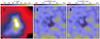 |
Fig. 3 Results of a test with a single Gaussian distribution of intrinsic colours. The leftmost frame shows the input map of AJ that is convolved to 3′, the resolution of the calculated extinction maps. The other frames show the difference between the estimated and the true extinction values for NICER (frame b)) and SCEX Method B (frame c)). The negative values around the column density peak indicate bias that is related to extinction gradients. |
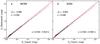 |
Fig. 4 Results of Fig. 3 as scatter plots and as NICER and SCEX estimates as functions of the input AJ (convolved to 3′). The frames include values of the bias Δ ( |

4.2. Complex distribution of reference colours
SCEX should present some advantages if the distribution of intrinsic colours is more complex than the single 2D Gaussian of the previous test (Sect. 4.1). To examine this in practice, we simulated intrinsic colours consisting of three Gaussian distributions. The distribution is basically ad hoc but has some resemblance to a mixture of stellar populations and galaxies with redder colours. The example is chosen explicitly to represent a case where the differences between the methods should be clear. The distribution of intrinsic colours and one realisation of stars in the ON field (knoise = 0.3) are shown in Fig. 5.
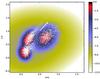 |
Fig. 5 Probability distribution of reference colours (colour image and logarithmic colour bar) in the second test case. The white arrow points in the direction of the reddening vector, the length corresponding to an extinction of AJ = 1.0 mag. The white dots show one realisation of reddened observed colours. The larger white circle indicates the mean intrinsic colours. |
4.2.1. The basic method
Figure 6 shows the NICER and Method B estimates in relation to the true AJ values of the simulation. Method B has smaller errors especially in low column density regions, and the improvement can be attributed to the use of a more accurate description of the intrinsic colour distribution. Both methods underestimate the extinction around the column density peak. Calculated over the whole map, the rms error and the bias of the SCEX map are some 40% lower. Because the rms values are strongly affected by the errors at high AJ, the differences are clearest below AJ ~ 1 mag.
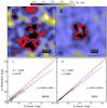 |
Fig. 6 Errors of NICER and SCEX (Method B) extinction estimates in test involving a complex distribution of intrinsic colours (knoise = 0.3). The upper frames show the difference between the calculated extinction maps and the input map convolved to the same 3.0′ resolution. Lower frames show the estimates as a function of the true AJ values. The numerical values of average bias Δ and rms errors σ are given in the figure. |
When noise is increased from knoise = 0.3 to knoise = 1.0, the difference between the methods is reduced. This can be expected because added noise makes the observed colour distributions more Gaussian. Considering the complexity of the simulated intrinsic colour distribution, NICER performs quite well, although the overall rms error of SCEX maps is still 20–25% lower. The bias of Method B is also smaller but this is a rather small effect, considering that in the colour–colour plane, the source populations are separated by AJ ~ 1 mag along the reddening vector. If the noise is increased further, the distribution of intrinsic colours (including magnitude errors) approaches a single Gaussian, and the difference between NICER and SCEX slowly vanishes.
4.2.2. Template of AJ variations
The method T makes use of an input template of the AJ variations on scales below the beam size (see Sect. 2.1). In the first test we used the true AJ map at 1.0′ resolution. The method needs the ratios of AJ values along individual lines of sight relative to the value in a map convolved to the resolution of the final extinction map. In simulations the correct ratios can be easily extracted from the input data, which represent perfect knowledge of all small-scale structure. This idealised case indicates the maximum potential benefit from this method. As emphasised in Sect. 2.1, the added information only concerns the relative extinction values within each beam separately and does not directly affect either the absolute or relative pixel values of the resulting AJ maps.
Figure 7a shows the that knowledge of the small-scale structure does have a very significant effect on the accuracy of the extinction estimates. While the rms error of NICER was σ = 0.11, the errors of Method T are smaller by almost a factor of ~5. This is also almost a factor of three below Method B errors in Fig. 6. The systematic errors are almost completely removed, because the least squares slope (between estimated and true values) is ~0.99 compared to 0.87 for Method B and 0.81 for NICER.
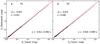 |
Fig. 7 SCEX Method T results plotted against the true values. SCEX calculations use either accurate knowledge of small-scale AJ variations (Method T1, frame a)) or use the NICER extinction map as a template of those variations (Method T2, frame b)). The average bias Δ and rms errors σ, as well as the parameters of least square lines (estimates vs. true values) are given in the frames. |
We argue in Sect. 2.1 that accurate information of sub-beam structure could be available from observations at other wavelengths. However, we also consider the possibility of using the AJ map itself as the input template. In this case, the template contains no information of real small-scale structure, but it does contain some information of large-scale extinction gradients. In practice, we estimated extinction variations with the NICER map, using the ratios between the values of individual pixels and smoothed estimates obtained by convolving the same map with a beam of 3′. In other words, we are estimating the extinction variations using the ratio of 4.2′ and 3.0′ maps instead of the ideal case of 3′ resolution vs. infinite resolution.
The result of the test with the NICER input map is shown in Fig. 7b. The results are worse than when perfect knowledge of the small-scale structure was available. However, the errors are only half of what they were for Method B (e.g., the slope of the least squares fit is 0.96 for Method T and 0.87 for Method B). The errors are greatest at the highest AJ values, where Method T underestimates the true extinction. This is natural because the template does not have the resolution to probe AJ variations at the peak, and therefore, the errors seen in Fig. 6 are only partially eliminated.
One might expect some improvement if using as input the corresponding deconvolved extinction map that could predict larger sub-beam column density variations at the location of the main peak. We tested this using a deconvolved NICER map (three iterations with van Cittert algorithm). However, this resulted in no improvements. Although the deconvolved map appeared to give a good description of the most compact structures, the bias of the highest AJ values was not reduced. We went even further to feed the deconvolved result of the extinction calculation in as the template map of the next iteration but without any significant improvement. It is still possible that a deconvolved template map might work better in other circumstances, such as when higher stellar density allows more reliable deconvolution.
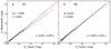 |
Fig. 8 Results of Methods D1 and D2 for the same case as in Fig. 6. Calculations with Method D1 assume a log-normal model with a standard deviation of σ = 0.5 for column density fluctuations. |
4.2.3. Corrections for bias
Apart from Method T, none of the above calculations make any correction for the fact that the probability distribution of the extinctions of detected stars is not symmetric with respect to the true beam-averaged extinction. In Method D1, we pre-calculated these probability distributions based on the OFF field statistics and included them as part of the calculation. The simulation is still based on the intrinsic colours shown in Fig. 5.
Figure 8a shows the result for Method D1 when the column density fluctuations are assumed to follow a log-normal distribution with standard deviation σ = 0.5. Compared to Method B, the rms errors are slightly smaller, but disappointingly the least squares slope between the estimated and true extinction values has increased only marginally from 0.87 to 0.90. If the value of σ is increased, the slope gets systematically steeper, but the estimates become unbiased only with a much higher value of σ ~ 1.2. Although the magnitude of the expected sub-beam fluctuations is not completely an ad hoc parameter, it cannot be determined directly from observations without higher resolution data. Furthermore, the statistics of the fluctuations can change across a map (e.g., between turbulence-dominated and gravitation-dominated regions). The column density distribution of the map used in this test is in fact very far from the assumed log-normal shape. On the high column density side, the distribution has a long power-law tail that also extends down to values well below the mean column density. This partly explains the poor performance of Method D1 in Fig. 8a.
Method D2 is essentially the same as the NICEST method, except for the use of a discretised PC distribution. For α we use a value α = 0.31 (cf. Juvela & Montillaud 2016). In the case of Fig. 8b, Method D2 shows practically no bias, and the least squares slope between D2 estimates and true extinction values is 0.99. The rms errors are lower than for Method B but higher than for Method T. In this case values of individual stars were calculated completely independently, making the calculation quite straightforward. If there was more significant ambiguity in the values (caused by multiple maxima in the intrinsic colour distribution), it might still be beneficial to include penalty for the dispersion of values within a beam. This would force all estimates to converge to a consistent solution before the final beam-averaged extinction estimate is calculated. Directly using NICEST with an assumption of Gaussian-distributed intrinsic colours results in some improvement over NICER (see Fig. 9) but still large bias compared to Method D2.
4.2.4. Case of two source populations
As the first test of cases of multiple pre-classified source populations, we classified the sources of Fig. 5 to two main components, with the sources found around (H−K, J−H) = (0.8,1.0) forming one component. The classification is assumed to take place before SCEX calculation, based on external information. We also assume that the intrinsic colour distributions are known for both populations separately. In practice, we use the same input catalogues as before but tag each source based on its known category. Because the generated source populations are well separated in colour–colour space, the noise of the two PC arrays is similar to the noise in the previous single PC array. The calculations of Method P correspond to Method B except for the use of two PC arrays. In particular, no steps are taken to correct for the bias (cf. Sect. 4.2.3).
Figure 10 shows that the explicit treatment of the two populations has reduced both the rms error and bias but not by much. Compared to Method B in Fig. 6, the overall bias has decreased from − 0.050 mag to − 0.043 mag, and the rms error has decreased from 0.064 mag to 0.055 mag. In the present case, each beam is likely to contain several sources from both populations so that when Method B fits a single AJ value, the result is already unique. If the solution assigned sources of one category to a wrong peak in PC, the sources of the other category would fall completely outside the distributions, resulting in a very low overall probability. Therefore, the advantage of Method P should be greater if the populations overlap in colour–colour space so that there is a greater risk of confusion or if the number of sources per beam is so small that, without a priori information of their category, they could all be attributed to either of the two source populations.
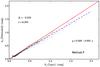 |
Fig. 10 Result of Method P, using a priori classification into two source populations. |
4.3. Tests using Besançon simulations
The final test uses a more realistic case where the intrinsic colours are obtained from the Besançon stellar population model (Robin et al. 2014). The synthetic catalogue only consists of stars, but their colour distribution depends on Galactic location and apparent magnitude. We used the data as shown in Fig. 1, which corresponds to coordinates (l, b) = (10°, 20°). As illustrated by the figure, the colour–colour distribution is elongated and changes significantly as a function of apparent magnitude. If the photometric accuracy of the observations is very high, this information could be used in calculations to define probability distributions separately for different magnitude intervals. To emphasise the potential differences between the methods, we simulated very deep observations with low photometric errors. The completeness limit is set around 23 mag in the H-band, and the photometric errors are 0.1 times the typical 2MASS errors (knoise = 0.1). Such observations may be impossible for current ground-based instruments but may become possible in the near future either with ELT1 or space-borne instruments2. Results of the tests conducted in this section are summarised in Fig. 12.
Figure 11 shows the results for NICER and Method B. For the realisation used in these tests, the reference NICER solution has a bias of − 0.08 mag and an rms error of 0.06 mag. Method B results in a bias of 0.02 mag and an rms error of 0.04 mag. The rms value of Method B is smaller mainly because of the good performance below AJ ~ 0.5 mag. The absolute accuracy of Method B estimates is also better at high extinctions, the comparison with the input extinction map giving a linear slope of ~1.0. For both methods, the largest errors are concentrated near the extinction maximum. As already discussed, this is caused by column density gradients and results from the false model assumption of a constant extinction across the beam.
Although not evident in these tests (or in Sect. 4.2), Method B could encounter some problems when intrinsic colours are concentrated along a very narrow ridge in the colour–colour plane. If probability drops very fast outside the ridge, a single star (observed through an extinction that is slightly different from the beam-average value) can have a strong influence on the estimate of the beam-averaged extinction. Methods like Method T should be more robust because they explicitly include sub-beam extinction fluctuations as part of the model, and a crude fix would be to convolve PC to accommodate some small-scale variations in AJ. However, as shown by Fig. 1, in practice this was not a significant problem.
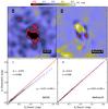 |
Fig. 11 Comparison of NICER (left) and Method B (right) results in the case of stars simulated with the Besançon model. The upper panels show maps of absolute error ΔAJ and the lower panels the correlations between recovered and true AJ values. |
Tests in Sect. 4.2.2 show that the small-scale column density variations are a significant source of noise in the extinction maps. If the relative AJ values within the beam are known, Method T drastically reduces the errors (see Fig. 12d). For the same realisation as above, the rms noise is reduced by a factor of four and the estimates remain accurate up to the largest column densities. The average bias is 0.008 mag, smaller than for Method B, which already was quite close to zero. Because we use here the true extinction map as an input, it is not something that could be applied to real observations, at least not without reliable, high-resolution ancillary data (see Sect. 2.1). If we use the NICER extinction map as a template of the small scale structure (mainly gradients), the improvement of rms noise is still quite significant, a factor of two over Method B (Fig. 12e). These estimates remain accurate even near the central peak.
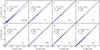 |
Fig. 12 Correlations between estimated and true extinction in tests with stars simulated with the Besançon model. Results are shown for NICER (frame a)), Method B (frame b)), Method B with separate reference colours for four magnitude intervals (frame c)), Method T using a perfect extinction template (frame d)), or using the NICER map as the template with a single (frame e)) or four reference colours (frame f)). The final frames include bias correction with methods D1 and D2 (frames g) and h), respectively). Each frame lists the parameters of linear least squares, the bias Δ, and the rms error σ. |
We also tested Method P, using separate PC distributions for stars in the apparent magnitude intervals <15, 15–19, 19–22, >22 mag. The limits are selected so that a roughly equal number of stars falls within each category (apparent magnitudes without extinction). With the subdivision Method P results in bias Δ = −0.003 mag and rms error σ = 0.042 mag, with a least squares slope of 0.97 (Fig. 12c). In other words, the result is slightly worse than with Method B and a single PC distribution. This may be because, once the reference stars are divided to four samples, each individual PC map has somewhat higher noise. Using the same four categories with Method T and NICER template results in a bias of Δ = 0.006 mag and an rms noise of σ = 0.016 mag (Fig. 12f), close to the result obtained using Method T and a single PC probability distribution. Thus, in the case of these more realistic colour–colour distributions, there does not appear to be any advantage in using multiple PC distributions.
This may be surprising considering the large variation seen in Fig. 1 and the degeneracy of solution for any star located either in the horizontal or in the vertical branch of that figure. In our test most stars are in the horizontal part, but each beam also contains many stars so that the value of the beam-averaged extinction is not ambiguous. The presence of stars in both branches always defines a unique solution. If the stellar density were very low, the a priori information provided by the apparent magnitude could be expected to become more important.
Methods D1 and D2 try to reduce bias without explicit information of sub-beam column density structures. In Fig. 12 Method B results were already almost unbiased and neither D1 nor D2 results in clear improvement. The least squares slope between estimated and true extinction is 1.02 for both D1 and D2. The scatter σ is similar to Methods B and thus larger than for Method T.
4.4. Summary of results on simulated observations
The previous tests show that if the distribution of intrinsic colours is not approximated well with a Gaussian distribution, it is useful to use a discretised representation to retain full information of the distribution. Figure 13 summarises the results for the colour distributions discussed above, one consisting of three Gaussian components and the other one based on stars simulated from the Besançon model. Figure 13 shows a series of calculations with decreasing stellar density. In the previous examples the number of stars was 5000 over the map area. In Fig. 13 we decrease the number of stars in steps of 1000 down to 1000 stars per map. At the same time we change the detection threshold so that each step corresponds to a 1.0 mag increase in the value of the limiting magnitude (removal of the faintest stars). The simulations with 2MASS stars start with the original completeness curves of the survey. In the original distribution of Besançon stars, the faintest stars are ~24.5 mag in H-band, but because of the completeness curves applied in the simulations, the peak in the counts is for more than 0.5 mag brighter stars. Because the intrinsic colours depend on the apparent magnitude, a change in the detection threshold also means a change in the average colour (cf. Fig. 1).
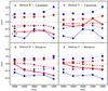 |
Fig. 13 Comparison of rms error σ (squares), bias Δ (triangles), and least squares slopes k (circles; error is k−1.0) for NICER (blue symbols and lines) and SCEX (red symbols and thick lines) as a function of stellar density. Each decrease of 1000 stars per map also corresponds to an increase of 1.0 mag in the limiting magnitude. |
Figure 13 shows that the rms error (measuring difference of the recovered extinction map and the true input map) is always lower for Method B than for NICER. The difference is greater in the case of colour–colour distributions consisting of three Gaussians, i.e., strong deviation from a distribution that could be approximated with a single covariance matrix. Compared to Method B, Method T again performs consistently better. The improvement is most noticeable in the bias (average difference between estimated and true extinction) and in the slope of the least square fits that compares extinction estimates with the known true values. The change from 5000 to 1000 stars per map does not cause a very strong increase in errors, and in most cases the increase shows a similar rate for both NICER and Methods B and T. One exception is seen for simulated Besançon stars where the Method B (and to some extent Method T) estimates start with a much lower bias but approach the NICER bias values as the number of stars is decreased. It is important to note that a decrease in stellar density is associated here with the removal of the faintest stars that have a colour distribution that is very different from the brighter stars. Thus, the remaining stars have more similar colours.
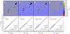 |
Fig. 14 Residuals for extinction maps calculated for the Pipe Nebula at a resolution of 300″. The reference is the Lombardi et al. (2006) NICER map that has been convolved to the resolution of 300″ (see text). Residuals are shown for NICER (frame a)), Method B (frame b)), and Method T (frames c) and d)). Method T uses the NICER map of frame a (frame c)) as a template of the small-scale structure or the Lombardi et al. (2006) NICER map at the full 60″ resolution (frame d)). Frames d)–g) show the corresponding data as scatter plots with the reference data on the x-axis. The maps are in Galactic projection and have a size of 3.22 × 3.22 deg. |
4.5. Application to real observations
As a final test we examine extinction maps of the Pipe Nebula. The NICER maps of the region are available already on line3, since the calculations are based on stars from the 2MASS survey (see Lombardi et al. 2006). These maps have a resolution of 1.0′ and a pixel size of 30″. We compare calculations where the distribution of intrinsic colours is derived either from 2MASS stars in a reference region or from the Besançon model.
We start by using reference colours estimated with ~46 000 2MASS stars in the vicinity of Galactic coordinates (355.97, 8.00). Because of the large photometric errors (compared to those used in Sect. 4.3) the reference colours can be approximated with a 2D Gaussian, and results of Method B are expected to be similar to those of NICER. For the same reason, the use of several PC distributions is not likely to be relevant. Therefore, we concentrate on Method T.
Figure 14 shows the results for extinction maps calculated at a resolution of 300″. The large beam size was selected because in this case, the results are expected to show significant bias and underestimate the extinction of the dense clumps. The results are compared to the NICER map originally calculated at 60″ resolution and then convolved to the 300″ resolution. As expected, NICER and Method B give rather similar results, although the slope of the linear fit is 0.03 units lower for Method B, and this suggests that PC can in this case be approximated with a single Gaussian. Both methods underestimate the extinction of the reference map, the error at the highest extinction reaching ~30% when compared to the reference, which is the Lombardi et al. (2006) map convolved down to the 300″ resolution. Method T (frames c and f) shows improvement over NICER and Method B. The rms error is lower by ~30%, and especially the bias of the highest extinction values has decreased. In frames c and f, the template was the NICER map that was convolved to a resolution of 300″. The last frames of Fig. 14 show the results when the template is the reference map with a 60″ resolution. In this case the slope of the linear fit is very close to unity.
We repeat the calculation by extracting PC from stellar catalogues simulated with the Besançon model for the centre of the field. In Fig. 15 the reference (x-axis of the scatter plots) is again the Lombardi et al. (2006) NICER map convolved to 300″ resolution. In Fig. 15a our NICER map uses the same simulated reference stars as the SCEX calculations, which accounts for the difference between frames d of Figs. 14 and 15.
In Fig. 15 the absolute extinction values are lower than in Fig. 14. For the first time, Method B appears to perform worse than NICER. We believe this to be a sign of problems in the description of reference colours. Based on simulated stars, PC is constructed directly, and the distribution of intrinsic colours is narrower than the colours of the actual stars in the field (almost a factor of two difference when measured along the H–K axis). This is also thus true in a direction perpendicular to the reddening vector. For stars outside the expected colour–colour distribution, the calculated probabilities will correspond to the tail of the PC probability distribution, i.e., the tail of the Gaussian kernel that was used to convert simulated stars into a continuous PC distribution (see Sect. 2). The probability gradients along the reddening vector are therefore largely arbitrary for those stars whose intrinsic colours are outside the assumed colour–colour distribution. The situation is somewhat different for NICER, where the distribution of intrinsic colours is described with a single 2D Gaussian, which is also affected by the general shape of the colour–colour distribution and not only by the local probability profile along a given reddening vector. In the present case the mismatch between PC and the distribution of observed stars is fairly obvious. Nevertheless, the result suggests that NICER may be generally more robust against this type of inaccuracy.
In Fig. 15, even Method T does not show any improvement over NICER when the 300″ resolution NICER map is employed as a template. Only when the template with 60″ resolution is used are the results finally better in terms of both the scatter σ and the slope of the least squares line. The improvement is most significant for dense clumps.
In the case of Fig. 15, one must remember that the reference (x-axis of the scatter plots) is a NICER calculation where the intrinsic colours are derived from observations of a real reference field. Therefore, some of the differences are caused by the different assumptions of the intrinsic colours.
Figure 16 shows the correlation between extinction estimates calculated with Method B with reference colours extracted from the Besançon model at two reference positions. The positions correspond to the main clumps within the map area and are separated by a distance of 2.2 deg (1.5 deg in Galactic latitude). The figure shows that the gradient of intrinsic colours results in a zero-point shift that is less than ΔAJ = 0.1 mag over the whole field. Nevertheless, if the effect is neglected, this causes an observable gradient over the extinction map. The effect is ≳10% for all values below AJ = 1.0 mag, causing the calculated extinction to drop slightly too fast as a function of Galactic latitude. Second, the rms scatter between the two calculated extinction maps is 0.7%. This is caused in part by noise in the reference colour distributions (derived from a finite sample of simulated stars) but shows an upper limit for the Monte Carlo noise in our calculations.
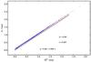 |
Fig. 16 Comparison of Method B with reference colours based on the Besançon model. The colours correspond to two locations along the filament, one below the central latitude (x-axis of the figure, reference position l = 358.8, b = 5.6) and one near the northern end (y-axis of the plot, reference position l = 357.1, b = 7.1). |
5. Discussion
We have examined extinction calculations with the observed NIR colours of background sources. The starting point was the premise that instead of using a single covariance matrix to describe the distribution of intrinsic colours of the sources, it may be better to operate with discretised probability distributions. We studied the use of three near-infrared bands, using observed J−H and H−K colours and their expected distribution in a 2D colour–colour plane. Within the MCMC framework we have tested several modifications that might be useful. In particular, these include (1) use of prior information on small-scale column density structure; (2) debiasing using a model for the statistics of column density variations or using a NICEST type correction; and (3) division of sources into subcategories, for example, based on apparent magnitudes.
The tests confirmed that when the distribution of intrinsic colours is approximately Gaussian, the methods recover the same result as NICER calculations (e.g., Fig. 4). Some differences should arise already if the distribution of intrinsic colours is skewed, and this also depends on our decision to use the median value of MCMC samples as the extinction estimate. The tests in Sect. 4.2 were chosen to create conditions where the difference to the simple Gaussian approximation is very pronounced. If a large number of the sources were galaxies that cannot be filtered out prior to the extinction analysis, the situation would be rather similar to that of Fig. 5. The first conclusion of these tests is that, in spite of the wrong assumption (regarding the distribution of intrinsic colours), NICER results remain quite accurate. Nevertheless, Method B shows noticeably lower rms noise, especially at low extinctions. The quantitative results also depend on the structure of the column density distribution. Both methods underestimate the extinction in regions of strong extinction gradients. If the photometric errors are increased or the intrinsic colour distribution is more Gaussian, the differences in the noise at low column densities disappear. This is also the case for the actual observations shown in Figs. 14, 15. In tests like the one shown in Fig. 6, the noise of NICER and SCEX maps is also similar at higher column densities where the errors appear to be dominated by the random sampling by background stars rather than the uncertainty of the intrinsic colours.
In the presence of column density gradients, the estimates of Method B are biased downwards, and the errors are similar to those of NICER maps. One of the most promising improvements of Method B is the use of ancillary information on sub-resolution variations in extinction. Method T uses the ratio of extinction along a given LOS (a single star) and the average extinction over a beam. Therefore, the estimated extinction values remain independent of the scaling of the ancillary data, and only estimates of relative extinction values are needed. Furthermore, the ratios are calculated independently for each beam, again avoiding any direct link between the large-scale morphology of the reference data and the estimated extinction map.
In Method T, the explicit inclusion of information on the small scale was seen to also be very effective in decreasing the bias. Although perfect knowledge of sub-beam structure can be expected to improve the accuracy of extinction estimates, its impact is still surprisingly large (see Fig. 7). This is particularly clear when the photometric errors are small and most of the noise results from small-scale column density variations. When the extinction map itself is used as the reference, the correction is still usually effective, especially if the column density variations are mostly caused by large-scale gradients that are also resolved by low-resolution extinction data. In Fig. 7, at low column densities, the errors are a fraction of the corresponding errors in NICER. When the reference data fail to resolve important column density peaks, the errors are still smaller than for NICER, but the scatter is higher, and the estimates are biased towards lower values. The only case where Method T did not produce clear improvements is shown in Fig. 15f. However, when the template map had a higher resolution, Method T also performed well in this test.
High-resolution estimates of column density can be available from various sources, such as molecular line or dust continuum observations. For example, Herschel observations cover most of the nearby molecular clouds, providing dust column density maps down to a resolution of 18″ resolution or even better. If the resolution of extinction maps is at most ~1′, this should be enough to provide significant improvement in the accuracy of extinction estimates. On the other hand, in the case of deep NIR observations, the resolution of extinction maps themselves may be so high that no higher resolution reference data exists. However, even the use of extinction data itself can sometimes result in a significant improvement in accuracy (e.g., Fig. 7b).
The changes in the distribution of intrinsic colours (e.g., Fig. 1) have suggested that extinction estimates could be improved by considering the differences in the intrinsic colours of stars of different apparent magnitudes. In practice no clear improvement was observed. We suspect that the main cause is that, as long as there are many stars within the beam, the solution is well constrained even without this additional information. For an individual star, there may be more than one possible solution along the reddening vector. For example, in Fig. 1 an unextincted star might reside either in the horizontal part (low extinction) or in the vertical part (much higher extinction) of PC. If the beam contains a single star, Method B returns the median of the probability distribution, which in this case contains two peaks. Thus, the estimate is likely to be either clearly too low or clearly too high (similar to NICER if one approximates the intrinsic colour distribution with a single Gaussian). However, as soon as the beam contains stars originating in both the vertical and the horizontal parts of the distribution, the solution of the beam-averaged extinction becomes unique. Furthermore, the stars in different magnitude intervals do not have entirely different intrinsic colours. They simply fill in parts of an already well-constrained common probability distribution. Thus, the situation is similar to Sect. 4.2 where it is not necessary to know beforehand which population an individual source belongs to. The situation could change if the number of sources per beam is very small so that all sources could by chance belong to one of the two populations.
We also tested Method D1 where the probability distribution between the beam-averaged extinction and the extinction seen by an individual star was explicitly taken as a part of the model. In Method D1, the asymmetry of this distribution was established using the cumulative star numbers and an assumption of the column density statistics. The method should reduce the bias caused by sub-beam column density variations. The main weakness of this method is that the magnitude of the correction directly depends on the assumed magnitude of the column density fluctuations. In the practical tests, Method D1 did not result in significant improvements. On the other hand, Method D2 implements the principles of the NICEST method (Lombardi 2009). The correction only depends on the extinction estimates calculated for individual stars, i.e., on observable quantities. In tests, Method D2 resulted in some improvement (especially in Fig. 8b), but it can also lead to increased rms errors (see Fig 12h).
MCMC has the advantage of providing estimates of the full posterior probability distribution of extinction. On the other hand, the computations are slower, in some cases by orders of magnitude, compared to NICER or NICEST methods. However, all methods discussed in this paper could also be used in connection with faster least squares or optimisation methods (e.g., on top of existing NICER or NICEST implementations; see A). This would reduce, although not eliminate, the difference in computational time but would also reduce the information we have of the parameter distributions. In this context, it is also interesting to examine the actual posterior probability distributions of the extinction values. Figure 17 shows examples for Methods B and T. Because of the way the photometric errors were included in calculations (see Sect. 2), the ratios of calculated probabilities are not strictly correct. This affects the width of the posterior probability distribution, therefore Fig. 17 should be taken only as a qualitative indication of the differences in these distributions. At low extinction values, which in this case also correspond to a relatively constant extinction across the beam, the distributions are almost Gaussian. Larger deviations from normal distribution are seen for the high extinction (and high AJ gradient) pixels. As indicated by the rms values, Method T results in smaller uncertainties. This is also associated with a more Gaussian probability distribution as the long tail to lower extinction values is decreased. This suggests that especially with Method T, faster calculations (least squares instead of MCMC) would not necessarily result in a significant loss of information.
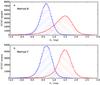 |
Fig. 17 Probability distributions for the extinction in two individual pixels (blue and red histograms) in the maps discussed in Sect. 4.2. Distributions are shown for Method B (upper frame) and Method T (lower frame) for the same pixels. |
6. Conclusions
We have examined the calculation of extinction based on the colours of background stars. We characterised the colours of unextincted stars using a full 2D probability distribution, instead of the conventional Gaussian approximation. We examined several variations of the basic method. The study led to the following conclusions:
-
By replacing Gaussian approximation with a more accuratedescription of intrinsic source colours, one can significantlyreduce the noise of the extinction maps. If the sources only consistof stars, photometric errors can eliminate most of this advantage.However, a precise description of the intrinsic colours will beimportant in case of high-precision measurements from futureinstruments such as ELT or WISH.
-
The largest improvements are obtained by including a priori information about the small-scale column density structure (Method T). This could be in the form of higher resolution observations of dust emission. However, by tracing the large-scale gradients, the information contained in the extinction data itself is sometimes sufficient to significantly reduce both the bias and the noise of the extinction estimates.
-
Method D2 can be very efficient in correcting the bias of extinction maps. This has already been demonstrated before because, apart from the use of a discretised intrinsic colour distributions, the method is similar to NICEST. However, if a good template map is available (one with low noise and preferably high resolution), Method T can result in an equally low bias and smaller rms errors.
We carried out the computations using the Markov chain Monte Carlo program SCEX. However, the ideas can be used just as well in connection with faster least squares or optimisation methods, making the methods more practical for analysing large areas.
Lombardi, Marco; Alves, Joao; Lada, Charles J. (2014), 2MASS extinction map of the Pipe Nebula, http://dx.doi.org/10.7910/DVN/25112 Harvard Dataverse Network V3.
Acknowledgments
This publication makes use of data products from the Two Micron All Sky Survey, which is a joint project of the University of Massachusetts and the Infrared Processing and Analysis Center/California Institute of Technology, funded by the National Aeronautics and Space Administration and the National Science Foundation. M.J. acknowledges the support of the Academy of Finland Grants No. 250741 and 285769.
References
- Alves, J., Lombardi, M., & Lada, C. J. 2014, A&A, 565, A18 [NASA ADS] [CrossRef] [EDP Sciences] [Google Scholar]
- Cambresy, L., Epchtein, N., Copet, E., et al. 1997, A&A, 324, L5 [NASA ADS] [Google Scholar]
- Cambrésy, L., Boulanger, F., Lagache, G., & Stepnik, B. 2001, A&A, 375, 999 [NASA ADS] [CrossRef] [EDP Sciences] [Google Scholar]
- Cambrésy, L., Beichman, C. A., Jarrett, T. H., & Cutri, R. M. 2002, AJ, 123, 2559 [NASA ADS] [CrossRef] [Google Scholar]
- Cardelli, J. A., Clayton, G. C., & Mathis, J. S. 1989, ApJ, 345, 245 [NASA ADS] [CrossRef] [Google Scholar]
- Davenport, J. R. A., Ivezić, Ž., Becker, A. C., et al. 2014, MNRAS, 440, 3430 [NASA ADS] [CrossRef] [Google Scholar]
- Dobashi, K., Uehara, H., Kandori, R., et al. 2005, PASJ, 57, 1 [Google Scholar]
- Foster, J. B., Román-Zúñiga, C. G., Goodman, A. A., Lada, E. A., & Alves, J. 2008, ApJ, 674, 831 [NASA ADS] [CrossRef] [Google Scholar]
- Górski, K. M., Hivon, E., Banday, A. J., et al. 2005, ApJ, 622, 759 [NASA ADS] [CrossRef] [Google Scholar]
- Juvela, M., & Montillaud, J. 2016, A&A, 585, A38 [NASA ADS] [CrossRef] [EDP Sciences] [Google Scholar]
- Juvela, M., Ristorcelli, I., & Marshall, D., et al. 2015, A&A, 584, A93 [NASA ADS] [CrossRef] [EDP Sciences] [Google Scholar]
- Lombardi, M. 2009, A&A, 493, 735 [NASA ADS] [CrossRef] [EDP Sciences] [Google Scholar]
- Lombardi, M., & Alves, J. 2001, A&A, 377, 1023 [NASA ADS] [CrossRef] [EDP Sciences] [Google Scholar]
- Lombardi, M., Alves, J., & Lada, C. J. 2006, A&A, 454, 781 [NASA ADS] [CrossRef] [EDP Sciences] [Google Scholar]
- Lombardi, M., Lada, C. J., & Alves, J. 2008, A&A, 489, 143 [NASA ADS] [CrossRef] [EDP Sciences] [Google Scholar]
- Lombardi, M., Lada, C. J., & Alves, J. 2010, A&A, 512, A67 [NASA ADS] [CrossRef] [EDP Sciences] [Google Scholar]
- Lombardi, M., Alves, J., & Lada, C. J. 2011, A&A, 535, A16 [NASA ADS] [CrossRef] [EDP Sciences] [Google Scholar]
- Lombardi, M., Bouy, H., Alves, J., & Lada, C. J. 2014, A&A, 566, A45 [NASA ADS] [CrossRef] [EDP Sciences] [Google Scholar]
- Padoan, P., Cambrésy, L., & Langer, W. 2002, ApJ, 580, L57 [NASA ADS] [CrossRef] [Google Scholar]
- Robin, A. C., Reyle, C., Fliri, J., et al. 2014, A&A, 569, A13 [NASA ADS] [CrossRef] [EDP Sciences] [Google Scholar]
- Skrutskie, M., Cutri, R., Stiening, R., et al. 2006, AJ, 131, 1163 [NASA ADS] [CrossRef] [Google Scholar]
- Wang, S., & Jiang, B. W. 2014, ApJ, 788, L12 [NASA ADS] [CrossRef] [Google Scholar]
Appendix A: All-sky NICER map employing Method T
As an example of implementing some of the discussed ideas outside the MCMC framework, we have expanded the previous
calculation of an all-sky NICER map (Juvela & Montillaud 2016) to employ Method T. A normal NICER map was first calculated on Healpix pixelisation (Górski et al. 2005) with a resolution of FWHM = 3.0′ and with resolution parameter NSIDE = 4096, which corresponds to a pixel size of ~0.86′. This map was then used as a template in a second calculation. When the values of individual stars were combined to calculate the estimate of the beam-averaged extinction A(J), the values were first scaled by the ratio  read from the template map. As discussed in Sects. 2.1 and 4.2.2, this is most useful for correcting large-scale gradients that are resolved by the template map. The previous extinction map cannot of course probe actual structure on scales below the beam size, and the correction is further limited by the pixel size, which is only a factor of three smaller than the FWHM of the final map.
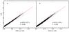 |
Fig. A.1 Comparison of our all-sky extinction maps A(J) and the (Lombardi et al. 2006) NICER map given as K-band extinction. The latter has been convolved from the original 1.0′ resolution down to 3.0′ resolution. The all-sky map has been calculated with the NICER method (frame a)) or with a modified method using Method T (frame b)). |
Figure A.1 compares the first NICER map and the second, Method T, map of the Pipe Nebula region. Both data are plotted against values from the (Lombardi et al. 2006) NICER map of the Pipe Nebula, which was originally calculated at a resolution of 1.0′ and was for this comparison convolved down to a resolution of 3.0′. As discussed in Juvela & Montillaud (2016), this should result in much lower bias than when a NICER map is calculated directly at a low resolution. In the latter case, which is applicable to our all-aky maps, the average extinction will be underestimated because the number of detected stars systematically decreases with column density. This is visible in Fig. A.1a, where at high column densities our values fall below the least squares line fitted to all data points. When Method T is used (frame b), the scatter of the relation increases but is more symmetric with respect to the least squares line, which is also somewhat steeper than in frame a. The relation remains linear up to the highest extinction values where the values are up to ~20% higher than with the basic NICER method. This suggests that Method T is able to improve the extinction estimates using only the photometry data, without any external information. When implemented in connection with NICER, the impact on computation times is minimal, and this enables calculation of large extinction maps.
All Tables
All Figures
|
Fig. 1 Stellar colours for Galactic direction (l, b) = (10°, 20°) for a sample of stars simulated from the Besançon model (Robin et al. 2014). The different intervals of J-band magnitude are plotted in different colours, as indicated by the values in the upper part of the figure. After the first one (8.0–11.0 mag), the subsequent sets of points are shifted by Δ(H−K) = 0.15 mag, for better readability. The smoothed contours are drawn at 10% and 50% of the maximum star density. |
| In the text | |
|
Fig. 2 Probability distribution of reference colours (colour image and logarithmic colour bar) in a test with a single Gaussian distribution of intrinsic colours. The white arrow points in the direction of the reddening vector, the length corresponding to AJ = 1.0 mag of extinction. The white dots show one realisation of the reddened stars in the ON field. |
| In the text | |
|
Fig. 3 Results of a test with a single Gaussian distribution of intrinsic colours. The leftmost frame shows the input map of AJ that is convolved to 3′, the resolution of the calculated extinction maps. The other frames show the difference between the estimated and the true extinction values for NICER (frame b)) and SCEX Method B (frame c)). The negative values around the column density peak indicate bias that is related to extinction gradients. |
| In the text | |
|
Fig. 4 Results of Fig. 3 as scatter plots and as NICER and SCEX estimates as functions of the input AJ (convolved to 3′). The frames include values of the bias Δ ( |
| In the text | |
|
Fig. 5 Probability distribution of reference colours (colour image and logarithmic colour bar) in the second test case. The white arrow points in the direction of the reddening vector, the length corresponding to an extinction of AJ = 1.0 mag. The white dots show one realisation of reddened observed colours. The larger white circle indicates the mean intrinsic colours. |
| In the text | |
|
Fig. 6 Errors of NICER and SCEX (Method B) extinction estimates in test involving a complex distribution of intrinsic colours (knoise = 0.3). The upper frames show the difference between the calculated extinction maps and the input map convolved to the same 3.0′ resolution. Lower frames show the estimates as a function of the true AJ values. The numerical values of average bias Δ and rms errors σ are given in the figure. |
| In the text | |
|
Fig. 7 SCEX Method T results plotted against the true values. SCEX calculations use either accurate knowledge of small-scale AJ variations (Method T1, frame a)) or use the NICER extinction map as a template of those variations (Method T2, frame b)). The average bias Δ and rms errors σ, as well as the parameters of least square lines (estimates vs. true values) are given in the frames. |
| In the text | |
|
Fig. 8 Results of Methods D1 and D2 for the same case as in Fig. 6. Calculations with Method D1 assume a log-normal model with a standard deviation of σ = 0.5 for column density fluctuations. |
| In the text | |
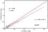 |
Fig. 9 NICEST result for the test same case as shown in Fig. 8. |
| In the text | |
|
Fig. 10 Result of Method P, using a priori classification into two source populations. |
| In the text | |
|
Fig. 11 Comparison of NICER (left) and Method B (right) results in the case of stars simulated with the Besançon model. The upper panels show maps of absolute error ΔAJ and the lower panels the correlations between recovered and true AJ values. |
| In the text | |
|
Fig. 12 Correlations between estimated and true extinction in tests with stars simulated with the Besançon model. Results are shown for NICER (frame a)), Method B (frame b)), Method B with separate reference colours for four magnitude intervals (frame c)), Method T using a perfect extinction template (frame d)), or using the NICER map as the template with a single (frame e)) or four reference colours (frame f)). The final frames include bias correction with methods D1 and D2 (frames g) and h), respectively). Each frame lists the parameters of linear least squares, the bias Δ, and the rms error σ. |
| In the text | |
|
Fig. 13 Comparison of rms error σ (squares), bias Δ (triangles), and least squares slopes k (circles; error is k−1.0) for NICER (blue symbols and lines) and SCEX (red symbols and thick lines) as a function of stellar density. Each decrease of 1000 stars per map also corresponds to an increase of 1.0 mag in the limiting magnitude. |
| In the text | |
|
Fig. 14 Residuals for extinction maps calculated for the Pipe Nebula at a resolution of 300″. The reference is the Lombardi et al. (2006) NICER map that has been convolved to the resolution of 300″ (see text). Residuals are shown for NICER (frame a)), Method B (frame b)), and Method T (frames c) and d)). Method T uses the NICER map of frame a (frame c)) as a template of the small-scale structure or the Lombardi et al. (2006) NICER map at the full 60″ resolution (frame d)). Frames d)–g) show the corresponding data as scatter plots with the reference data on the x-axis. The maps are in Galactic projection and have a size of 3.22 × 3.22 deg. |
| In the text | |
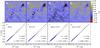 |
Fig. 15 As in Fig. 14 but using distributions of reference colours based on the Besançon model. |
| In the text | |
|
Fig. 16 Comparison of Method B with reference colours based on the Besançon model. The colours correspond to two locations along the filament, one below the central latitude (x-axis of the figure, reference position l = 358.8, b = 5.6) and one near the northern end (y-axis of the plot, reference position l = 357.1, b = 7.1). |
| In the text | |
|
Fig. 17 Probability distributions for the extinction in two individual pixels (blue and red histograms) in the maps discussed in Sect. 4.2. Distributions are shown for Method B (upper frame) and Method T (lower frame) for the same pixels. |
| In the text | |
|
Fig. A.1 Comparison of our all-sky extinction maps A(J) and the (Lombardi et al. 2006) NICER map given as K-band extinction. The latter has been convolved from the original 1.0′ resolution down to 3.0′ resolution. The all-sky map has been calculated with the NICER method (frame a)) or with a modified method using Method T (frame b)). |
| In the text | |
Current usage metrics show cumulative count of Article Views (full-text article views including HTML views, PDF and ePub downloads, according to the available data) and Abstracts Views on Vision4Press platform.
Data correspond to usage on the plateform after 2015. The current usage metrics is available 48-96 hours after online publication and is updated daily on week days.
Initial download of the metrics may take a while.