| Issue |
A&A
Volume 585, January 2016
|
|
|---|---|---|
| Article Number | A71 | |
| Number of page(s) | 41 | |
| Section | Interstellar and circumstellar matter | |
| DOI | https://doi.org/10.1051/0004-6361/201526238 | |
| Published online | 21 December 2015 | |
Outflow structure within 1000 au of high-mass YSOs
I. First results from a combined study of maser and radio continuum emission
1
INAF–Osservatorio Astrofisico di Arcetri, Largo E. Fermi 5, 50125
Firenze, Italy
e-mail: This email address is being protected from spambots. You need JavaScript enabled to view it.
2
I. Physikalisches Institut, Universität zu Köln,
Zülpicher Str. 77, 50937
Köln,
Germany
3
Department of Astrophysics, Institute for Mathematics,
Astrophysics and Particle Physics, Radboud University, PO Box 9010, 6500 GL
Nijmegen, The
Netherlands
4
Joint Institute for VLBI in Europe, Postbus 2, 7 9990 AA
Dwingeloo, The
Netherlands
5
Max-Planck-Institut für Radioastronomie,
Auf dem Hügel 69, 53121
Bonn,
Germany
6
Purple Mountain Observatory, Chinese Academy of
Sciences, 210008
Nanjing, PR
China
7
INAF-Istituto Fisica Spazio Interplanetario,
via Fosso del Cavaliere 100,
00133
Roma,
Italy
8
Harvard-Smithsonian Center for Astrophysics,
60 Garden Street, Cambridge, MA
02138,
USA
Received: 1 April 2015
Accepted: 11 September 2015
Abstract
Context. In high-mass (≥7 M⊙) star formation (SF) studies, high-angular resolution is crucial for resolving individual protostellar outflows (and possibly accretion disks) from the complex contribution of nearby (high- and low-mass) young stellar objects (YSO). Previous interferometric studies have focused mainly on single objects.
Aims. A sensitive survey at high angular resolution is required to investigate outflow processes in a statistically significant sample of high-mass YSOs and on spatial scales relevant to testing theories.
Methods. We selected a sample of 40 high-mass YSOs from water masers observed within the BeSSeL Survey. We investigated the 3D velocity and spatial structures of the molecular component of massive outflows at milli-arcsecond angular resolution using multi-epoch Very Long Baseline Array (VLBA) observations of 22 GHz water masers. We also characterize the ionized component of the flows using deep images of the radio continuum emission with resolutions of ~0."2, at 6, 13, and 22 GHz with the Jansky Very Large Array (JVLA).
Results. We report the first results obtained for a subset of 11 objects from the sample. The water maser measurements provide us with a very accurate description of the molecular gas kinematics. This in turn enables us to estimate the momentum rate of individual outflows, varying in the range 10-3–100M⊙ yr-1 km s-1, among the highest values reported in the literature. In all the observed objects, the continuum emission at 13 and 22 GHz has a compact structure, with its position coincident with that of the water masers. The 6 GHz continuum consists of either compact components (mostly well aligned with the 13 and/or 22 GHz sources) or extended emission (either highly elongated or approximately spherical), which can be offset by up to a few arcseconds from the water masers. The unresolved continuum emission associated with the water masers likely points to the YSO location. The comparison of the radio continuum morphology to the maser spatial and 3D velocity distribution shows that five out of elevenhigh-mass YSOs emit a collimated outflow, with a flow semi-opening angle in the range 10°–30°. The remaining six sources present a more complicated relationship between the geometry of the radio continuum and water maser velocity pattern; therefore, no firm conclusions can be drawn regarding their outflow structure. In two sources, the 6 GHz continuum emission shows a highly elongated structure with a negative spectral index down to −1.2. We interpret this finding in terms of synchrotron emission from relativistic electrons accelerated in strong shocks, which indicates that non-thermal continuum emission could be common in high-mass protostellar jets. The Lyman continua derived from bolometric luminosities always exceed those obtained from the radio luminosities.
Conclusions. These first results suggest that collimated outflows or jets can be common in high-mass YSOs and, in a couple of cases, provide hints that magnetic fields could be important in driving these jets. To draw firmer conclusions, however, we await completion of the analysis for the entire sample of 40 high-mass YSOs.
Key words: ISM: jets and outflows / ISM: molecules / masers / radio continuum: ISM / techniques: interferometric
© ESO, 2015
1. Introduction
Although high-mass (M> 7M⊙) stars play a fundamental role in the evolution of the gas chemistry and stellar content of galaxies, their formation process is still obscure. In the case of low-mass star formation (SF), the standard scenario predicted by theoretical models and supported by observations involves disk-mediated accretion and ejection of a jet (i.e., a collimated wind) along the disk axis. However, high-mass young stellar objects (YSO) can reach the zero age main sequence (ZAMS) and start H-burning reactions while still embedded in their natal molecular cores and actively accreting material. According to early calculations, the intense stellar radiation of a new-born massive star would exert enough pressure to halt inflow and prevent further mass increase (Wolfire & Cassinelli 1987). Recent 3D radiation hydrodynamic simulations of high-mass star formation instead seem to indicate that accretion disks and collimated outflows could allow the formation of stars up to ~140 M⊙ (see, e.g., Kuiper et al. 2010). The disk geometry focuses the accretion flow onto the equatorial plane, allowing accreting material to overcome the strong radiation pressure and reach the stellar surface. These models also predict beaming of stellar photons into the lower-density outflow cavities, which helps alleviate radiation pressure in the equatorial plane (Cunningham et al. 2011). The work by Keto (2003, 2007) also demonstrates that the ionization of the stellar surroundings produced by the intense UV radiation of the massive star does not necessarily halt and reverse the accretion flow. For high values of the mass accretion rate, the predicted size of the Hii region is so low that the stellar gravitational attraction dominates the thermal pressure of the ionized gas, and the Hii region does not expand.
A common feature of all SF models is the prediction of a tight connection between mass accretion and ejection. In low-mass SF, jets are generally modeled as magnetocentrifugally driven winds, powered by rotation and gravitational energy and launched along the magnetic field either from the inner edge of the disk (fraction of au; “X-wind”, Shu et al. 1995) or across a much larger (up to a few 10 au) portion of the disk (“Disk-Wind”, Pudritz et al. 2005). In the case of high-mass YSOs, recent calculations indicate that magnetic fields could be less efficient than in low-mass YSOs in collimating outflows, since magnetic collimation could be weakened by gravitational fragmentation of the accretion disk and by thermal pressure of the ionized gas at the base of the jet (Peters et al. 2011). In addition, outflows from high-mass YSOs could be intrinsically less collimated if driven by the YSO’s radiation pressure rather than by coherently rotating magnetic fields (Vaidya et al. 2011). Finally, OB-type stars emit powerful stellar winds, and if these are also present during the accretion phase (as is likely), they could contribute to the observed outflows from high-mass YSOs.
It is therefore clear that the study of the geometrical and physical properties of neutral and ionized outflows from high-mass YSOs can be key to a better understanding of many fundamental aspects of high-mass SF, and they can ultimately allow us to ascertain whether the paradigm of the star formation through a disk and jet system holds for more massive stars as well. Single-dish surveys (Beuther et al. 2002; Wu et al. 2004; Zhang et al. 2005; Kim & Kurtz 2006; de Villiers et al. 2015) have demonstrated that powerful molecular outflows are ubiquitous in high-mass star-forming regions. However, their angular resolutions of between 5′′ and 30′′ (corresponding to linear scales of ≥104 au at distances of a few kpc) are about ten times higher than the scales for the clustering of multiple forming stars (~103 au), and generally insufficient to isolate the flow pattern produced by a single high-mass YSO. Thus, in most cases, only the complex spatial and kinematic distributions resulting from the superposition of several outflows are actually observed. However, these surveys have been useful in providing the integrated properties of the outflows from high-mass YSOs, establishing characteristic mass outflow rates of ~10-4M⊙ yr-1, momentum rates of 10-3M⊙ km s-1 yr-1, and mechanical luminosities of 10-1–102L⊙. These values are typically several orders of magnitude higher than toward low-mass YSOs and are in general well correlated with the bolometric luminosity of the region (see, e.g., Wu et al. 2004). More controversial is the interpretation of the results in terms of the flow geometry, although these observations seem to indicate that early B-type stars show on average more collimated outflows than late O-type stars (see, e.g., Beuther & Shepherd 2005). This feature has been interpreted in terms of an evolutionary sequence, with an increasing outflow decollimation resulting from the larger stellar ionizing flux and radiation pressure of a more massive star. However, the less collimated outflows observed in more luminous regions could simply be an effect of the insufficient angular resolution, if a large number of unresolved YSOs contribute to the observed outflow pattern.
Besides single-dish surveys, there have also been some targeted interferometric studies of massive outflows at mm wavelengths in typical molecular outflow tracers (12CO, 13CO, SiO, HCO+), achieving angular resolutions of ~1′′–10′′ (see Arce et al. 2007, for a review). These interferometric observations in some cases succeeded in isolating the outflow of the most massive YSO in the region, revealing an elongated and bipolar structure in the velocity-integrated emission of specific outflow tracers (see, e.g., Sollins et al. 2004; Cyganowski et al. 2011). In some sources, it has also been possible to study the change in the geometrical and physical properties of the flow along the elongation axis, providing evidence of a linear velocity-distance relation or “Hubble flow” (see, e.g., Cesaroni et al. 1999), jet precession (see, e.g., Shepherd et al. 2000), and/or episodic ejection (see, e.g., Beltrán et al. 2011). In a recent study, Zhang et al. (2014) used the Submillimeter Array (SMA) to observe a large sample of massive outflows in both the dust polarized emission and the 12CO (3–2) transition, finding that major axes of the molecular outflows do not appear to be correlated with the orientation of the magnetic fields in the associated molecular cores. Although mm interferometric observations have resolved some individual high-mass protostellar outflows, the sampled scales are tens to hundreds of times larger than the model-predicted disk size (~100 au) and, thus, insufficient for investigating the flow-launching region, as well as determining the physical nature (e.g., stellar- vs. disk-wind, ionized vs. neutral) and the geometry (wide-angle vs. collimated) of the engine powering the larger scale molecular outflow.
To overcome some limitations of previous surveys and better constrain models of high-mass star formation, we have identified three crucial elements. First, direct imaging on scales of hundreds of au is essential to derive the structure, dynamics, and small-scale physical conditions of circumstellar gas at the disk/outflow interface, as well as resolve individual outflows in a protocluster. Second, to obtain a full picture of the mass-ejection process, the investigation should include both molecular and ionized components of the outflows. Third, to establish common patterns in the evolution of massive YSOs, the study should include a statistically significant sample. With this in mind, we started an observational program of massive protostellar outflows, achieving unprecedented angular resolution and sensitivity.
This paper presents the survey and reports on the first results based on analysis of a subset of eleven targets in our sample. Section 2 describes the survey strategy, including the sample selection. Section 3 presents the continuum JVLA and maser VLBA observations, while Sect. 4 reports the analysis of these and archival infrared data sets. The observational results are presented in Sect. 5 and are discussed in Sect. 6. Conclusions are drawn in Sect. 7.
2. A high-angular resolution survey of massive protostellar outflows
In our survey, we complement multi-epoch VLBI observations of water masers (Sect. 2.1) with high-angular resolution deep imaging of radio continuum emission with the JVLA (Sect. 2.2) in a relatively large sample of massive protostellar outflows (Sect. 2.3).
2.1. 3D velocity field from water masers
Owing to their intense brightness (≥109 K), molecular masers can be targets of VLBI observations, which, when achieving milli-arcsecond angular resolutions, permit us to derive the proper motions of the maser “spots” (i.e., the single maser emission centers) and establish full 3D gas kinematics. In particular, water masers emerge from shocked molecular gas at the interface between the fast flow and the ambient material, thus efficiently tracing the structure of (proto)stellar outflows close to (within 10–100 au of) the high-mass YSO (Goddi et al. 2005; Goddi & Moscadelli 2006; Moscadelli et al. 2007, 2011, 2013b; Sanna et al. 2010b, 2012). Interestingly, VLBI studies of water masers toward individual high-mass star-forming regions, when combined with the morphology of radio continuum emission, have revealed patterns of motions, which in a very schematic way can be divided into two groups (although exceptions to this classification can be found):
-
I.
In O-type YSOs, hyper-compact Hii regions expand (likely driven by stellar winds), exciting and accelerating water masers in wide-angle flows (e.g., Moscadelli et al. 2007; Beltrán et al. 2007).
-
II.
In B-type YSOs, thermal (likely shock-excited) radio jets are responsible for the excitation of water masers in collimated bipolar flows (e.g., Moscadelli et al. 2011; Goddi et al. 2011).
The wide-angle or collimated flows observed at distances ≤100 au from the (proto)star, corresponding to cases I and II, respectively, might account for the different degrees of molecular outflow collimation noted on scales of 103–104 au in previous single-dish and/or interferometric surveys (e.g., Beuther & Shepherd 2005). In particular, these findings are suggestive of an intrinsic different degree of the outflow collimation associated with the protostellar mass and/or age. While this scenario is plausible, it is not the only possible interpretation. Some other studies of outflows with molecular masers have revealed more complex systems that cannot be uniquely associated with jet-like outflows or shell-like expanding winds. In this respect, the most notable example is the high-mass YSO Source I in the Orion BN-KL region, where SiO masers trace a rotating and expanding wide-angle disk wind within <100 au of the star (Matthews et al. 2010), while H2O masers indicate the “recollimation” of the wide-angle wind in a straight bipolar flow at radial distance from 100 up to 1000 au (Greenhill et al. 2013). Another intriguing case is the high-mass star-forming region W75N(B), containing two massive protostars, identified by two cm-wavelength continuum sources, VLA1 and VLA2, which are separated by only ~900 au and drive two very different types of outflows: VLA1 drives a stable collimated jet, whereas VLA2 has evolved from a wind-driven shell to a jet-like structure in only 16 years, as proven by a VLBI monitoring study of the water masers (Torrelles et al. 2003; Surcis et al. 2014). Therefore, W75N(B)-VLA2 provides a rather unique case of a short-lived, possibly episodic outflow phenomenon where a real-time transition from an uncollimated to a collimated flow is observed during the early stages of a massive star. Since both VLA1 and VLA2 are part of the same core and show radio continuum emission that is consistent with excitation by an early B-type star, environmental properties and/or stellar masses cannot explain the difference in outflow morphology.
These examples suggest that different physical processes could take place at the earliest stages of massive star formation. A statistical approach to the problem, i.e. by observing a larger sample of sources, then becomes crucial.
2.2. Structure and nature of ionized winds from radio continuum imaging
List of BeSSeL sources observed with the JVLA.
The ionized component of outflows can be studied with cm wavelength interferometric
observations at angular resolutions of ~0 1
(corresponding to linear scales of a few 100 au). While radio jets (i.e., ionized
collimated winds) are commonly observed toward low-mass YSOs (e.g., Anglada 1996), up to now detailed studies toward individual sources have
only reported a small number of jets associated with high-mass YSOs (e.g., HH80–81: Marti et al. 1993; CepA-HW2: Rodríguez et al. 1994; IRAS 16547−4247: Rodríguez et al. 2008; IRAS 16562−1732: Guzmán et al. 2010). For
a few of them (e.g., HH80–81: Marti et al. 1998;
CepA-HW2: Curiel et al. 2006), multi-epoch VLA
observations have succeded in measuring the proper motion of persistent emission knots
along the jet, deriving velocities of ~500 km s-1. The radio luminosity of the jets observed in low- and
high-mass YSOs appears to be correlated with both the YSO bolometric luminosity and the
momentum rate of the associated molecular outflow (Anglada
et al. 2015). The latter correlation could suggest that the jets are ionized by
the energetic photons produced in strong shocks rather than photoionized by the stellar
radiation (Rodriguez 1989). However, for the few
jets observed toward high-mass YSOs, the Lyman continuum calculated from the YSO
bolometric luminosity generally exceeds the value inferred from the radio luminosity
(Anglada et al. 2015; Guzmán et al. 2012), suggesting that stellar photoionization could
still be the main ionization process. We also note that most previous surveys of radio
jets, performed with the Very Large Array (VLA), reached a sensitivity threshold of a few
0.1 mJy. Therefore, the low detection rate of radio jets toward high-mass YSOs could
indicate that their typical radio flux is weaker than this threshold.
1
(corresponding to linear scales of a few 100 au). While radio jets (i.e., ionized
collimated winds) are commonly observed toward low-mass YSOs (e.g., Anglada 1996), up to now detailed studies toward individual sources have
only reported a small number of jets associated with high-mass YSOs (e.g., HH80–81: Marti et al. 1993; CepA-HW2: Rodríguez et al. 1994; IRAS 16547−4247: Rodríguez et al. 2008; IRAS 16562−1732: Guzmán et al. 2010). For
a few of them (e.g., HH80–81: Marti et al. 1998;
CepA-HW2: Curiel et al. 2006), multi-epoch VLA
observations have succeded in measuring the proper motion of persistent emission knots
along the jet, deriving velocities of ~500 km s-1. The radio luminosity of the jets observed in low- and
high-mass YSOs appears to be correlated with both the YSO bolometric luminosity and the
momentum rate of the associated molecular outflow (Anglada
et al. 2015). The latter correlation could suggest that the jets are ionized by
the energetic photons produced in strong shocks rather than photoionized by the stellar
radiation (Rodriguez 1989). However, for the few
jets observed toward high-mass YSOs, the Lyman continuum calculated from the YSO
bolometric luminosity generally exceeds the value inferred from the radio luminosity
(Anglada et al. 2015; Guzmán et al. 2012), suggesting that stellar photoionization could
still be the main ionization process. We also note that most previous surveys of radio
jets, performed with the Very Large Array (VLA), reached a sensitivity threshold of a few
0.1 mJy. Therefore, the low detection rate of radio jets toward high-mass YSOs could
indicate that their typical radio flux is weaker than this threshold.
In this respect, the new broadband receivers now available at the JVLA yield an rms noise figure (~10 μJy in ~10 min) that is about ten times lower than for previous VLA continuum observations. This implies that we are entering a new regime of exploration of radio jets from distant high-mass YSOs and indicates that large samples can be studied.
2.3. Sample selection from BeSSeL
Our sample of massive protostellar outflows is selected from the Bar and Spiral Structure Legacy (BeSSeL) Survey. The main goal of the BeSSeL Survey is to derive the structure and kinematics of the Milky Way by measuring the accurate positions, distances (via trigonometric parallaxes), and proper motions of methanol and water masers in hundreds of high-mass star-forming regions distributed over the Galactic disk (Reid et al. 2014). Maser distances are determined with an accuracy typically better than 10%, and absolute positions and velocities are accurate within a few mas and km s-1, respectively. Thus, the BeSSeL water maser dataset is also optimal for studies of molecular gas kinematics in high-mass star-forming regions.
About 100 water maser sources were observed under the BeSSeL program by mid-2013. Among the observed masers, we selected a sample to be studied in the radio continuum with the JVLA using the following criteria:
-
1.
Water maser emission consisting of many (>10) spots stronger than 1 Jy, to ensure a sufficiently good sampling of the flow kinematics.
-
2.
Source bolometric luminosity (see Sect. 4.2) corresponding to a ZAMS type B3–O7, to select preferably high-mass YSOs.
-
3.
Targets that, in previous surveys, were undetected or that only showed compact (size ≤1′′) and weak (flux ≤50 mJy) radio continuum emission, to exclude extended and more evolved Hii regions.
-
4.
Source distances less than 9 kpc, to be sensitive to the (photoionized) radio emission of all high-mass YSOs (M ≥ 7M⊙).
According to this criteria, we selected 40 massive protostellar objects. Table 1 reports their absolute positions, distances, maser velocities, and bolometric luminosities.
Coordinates, synthesized beams and rms noise level of the JVLA continuum images.
3. Observations and data reduction
3.1. JVLA observations
Our source sample was observed using the JVLA of the National Radio Astronomy Observatory (NRAO)1 in both A and B configurations. The first fourteen sources (indicated by names underlined in Table 1) were observed between October 2012 and January 2013 in A configuration (project code: 12B-044), in C, Ku, and K-bands, centered at 6.2, 13.1, and 21.7 GHz, respectively. The observations of the remaining 26 sources were performed between March and May 2014 at C and Ku-bands in A configuration, and between February and May 2015 at K-band in B configuration, under project 14A-133. In this paper we only discuss 2012–2013 observations.
Individual observing segments at each band lasted from 1 to 2.25 h and contained three to five targets grouped together on the sky (within 10°–15°). To maximize the uv-coverage for each source, the total on-source times of 15 min at C and Ku-band and 30 min in the K-band were divided into several 5 min scans. The primary flux calibrator was one of three sources: 3C 286, 3C 48, and 3C 147. For each target and band, a suitable phase-reference calibrator was selected from the list of the VLA calibrators to be strong (≥0.5 Jy) and compact (VLA calibrator code “A” or “B”) enough and offset from the target by less than 10°. Phase-reference calibrators were observed for two to three minutes before and after each group of target scans with a maximum separation of 15–20 min between the target and calibrator scans. All fourteen targets were succesfully observed in the C-band; in the Ku-band G012.91−0.26 was missed; and in the K-band data for only eight sources (excluding G000.67−0.04, G000.68−0.03, G005.88−0.39, G048.61+0.02, G074.04−1.71 and G075.76+0.34) were obtained.
We employed the capabilities of the new WIDAR correlator, which permits recording dual polarization across a total bandwidth per polarization of 2 GHz, by using two IFs, each comprising eight adjacent 128 MHz subbands. At 6 GHz and 22 GHz, we centered one IF at the frequency of the methanol (6668.5192 MHz) and water maser (22 235.0798 MHz), respectively. Correlating each 128 MHz subband with 128 channels, we achieved a velocity resolution of 45 km s-1 and 13 km s-1 at 6 GHz and 22 GHz, respectively. For a typical maser line width of 0.2–0.3 km s-1 for methanol at 6.7 GHz and 0.5 km s-1 for water at 22 GHz, a 1 Jy maser peak would be degraded by the coarse velocity resolution to 6 mJy for methanol masers and 40 mJy for water masers. However, such a signal is still detectable with high S/N (≥10–100) at both frequencies, since thermal noise in a 1 MHz channel is 0.3 mJy beam-1 at 6.7 GHz and 0.6 mJy beam-1 at 22.2 GHz.
This paper reports the results obtained for ten (with the name underlined and in boldface characters in Table 1) out of the fourteeen targets observed in 2012–2013. Water masers were detected in all sources, and methanol masers were detected in six out of the ten targets (see Sect. 5). When maser emission was either not recorded or detected, i.e., in Ku-band and for four sources in C-band, amplitude and phase corrections for the target visibilities were derived using the (primary and phase-reference) calibrators. When methanol or water masers were detected, we first applied the calibrator corrections to the maser channel and then self-calibrated the maser emission. Before mapping, we applied the same corrections to the continuum data. While self-calibration increased the S/N of the (dynamical range limited) maser images by a large factor (typically ≥10), it only marginally improved the (thermal noise-limited) continuum images. Based on the observing beams (see Table 2) and the self-calibrated maser S/Ns (≥100), the relative positions of the masers with respect to the continuum emission observed simultaneously, are accurate to a few mas.
Table 2 reports the beam parameters and the rms noise levels of the continuum images. We examined the absolute position differences between sources observed at different frequencies and on different days. The average position differences between C and Ku (or K) bands were 43 mas, whereas between Ku and K-bands they were 26 mas. This suggests that individual positions are good to about 40 mas in the C-band and 20 mas in the Ku and K-bands. The larger positional uncertainty for the C-band, compared to the higher frequency bands, probably stems from the greater impact of dispersive delay variations in the ionosphere.
In most cases, the rms noise level of the continuum image is close to the expected thermal noise: ~10 μJy beam-1 at 6 and 13 GHz and ~20 μJy beam-1 at 22 GHz. The C-band emission from two sources, G005.88−0.39 and G097.53+3.18, is extended and partially resolved by the A configuration, which explains the patchy structure of these images. Four of the observed sources, G011.92−0.61, G012.68−0.18, G075.76+0.34, and G097.53+3.18, show diffuse emission (size ~5′′–10′′) from nearby (within ~10′′–20′′) Hii regions. To improve the images of compact continuum sources associated with the water masers, we filtered out extended emission by imaging only with long baselines, selecting uv-projected lengths ≥50–200 kλ. In the Ku and K-bands, all sources show single or multiple compact components, except G005.88−0.39, which is completely resolved out at Ku-band.
For the purpose of determining the continuum spectral index (Sect. 5.2), for each target we produced images at each observed band using
the same uv-range (40–800 kλ), pixel
(0050)
and map (1024 × 1024 pixels)
size, and round beam (023).
These parameters were a compromise among the different uv-ranges and beams of the
three observing bands and allowed us to recover the main features of the continuum
emission in each band. For the four sources, G011.92−0.61, G012.68−0.18, G075.76+0.34 and G097.53+3.18, the same uv-limit as adopted for the
C-band
images was also employed for the images at the other frequencies.
3.2. BeSSeL VLBA water maser observations
All of our water maser sources have been observed as part of the VLBA BeSSeL survey (project code: BR145) at 6–9 epochs spanning about one year, with a total observing time per epoch of about seven hours. A general description of the BeSSeL VLBA observational setup is given in Reid et al. (2009). The data correlation was performed at the VLBA correlation facility in Socorro (NM, USA) using the DiFX software correlator (Deller et al. 2007) and employing an integration time of 0.9 s. The velocity resolution for the 22 GHz water maser data was 0.42 km s-1. Visibility amplitude and phase calibration were performed following the standard BeSSeL data reduction methodology (see, e.g., Reid et al. 2009). Before imaging, we self-calibrated on a strong and compact maser spot. We made spectral channel maps, typically covering several arcsec on the sky, for the velocity range (varying from source to source from 10 to 40 km s-1) where the signal was visible in total-power spectra. The CLEAN restoring beam was an elliptical Gaussian with typical half-power beam-widths (HPBW) of ~1 mas. The rms noise in channel maps varied from the thermal noise limit ≤10 mJy beam-1, for channels with no or weak emission, to ~500 mJy beam-1, for channels with strong signals.
4. Data analysis
4.1. Water maser kinematics
Our sample was observed with the VLBA and the data analyzed within the BeSSeL project2. The maser parallaxes and proper motions have been published for all ten of our targets but G097.53+3.18 (Immer et al. 2013; Xu et al. 2013; Choi et al. 2014; Sato et al. 2014). To achieve our science goals, we found it useful to analyze the datasets again. The main goal of BeSSeL is to map the structure and dynamics of the Milky Way, and as such it focuses on measuring the parallaxes and peculiar motions of individual maser sources, using only a few compact and intense (≥1 Jy) maser spots to perform the astrometric analysis. For our purposes it is important to include the largest possible number of maser spots, including relatively weak (~0.1 Jy) ones. This approach produces a better description of the circumstellar motions.
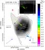 |
Fig. 1 Gray-scale image and contours: JVLA A-Array C-band continuum, using gray-tone steps that increase linearly with the map intensity from 8 mJy beam-1 to the peak emission of 82 mJy beam-1, and contours corresponding to 10% to 90%, in steps of 10%, of the peak emission. The extended Ku-band emission is totally resolved out by our JVLA A-Array observations, and this source was not observed in the K-band by the JVLA. Colored dots show the absolute position of individual maser features, with color denoting the maser VLSR, according to the color-velocity conversion code reported on the right side of the panel. The green color gives the systemic VLSR, derived through (single-dish and/or interferometric) observations in high-density, thermal tracers. Dot area is proportional to the logarithm of the maser intensity. Colored arrows represent the measured maser proper motions, with dotted arrows used to represent the most uncertain proper motions. The amplitude scale for the maser velocity is indicated by the black arrow in the bottom right of the panel. The white errorbars denote the position (with the associated error) of the bright star detected in the near-infrared with the VLT by Feldt et al. (2003), and the red and blue arrows indicate the direction of the red- and blue-shifted lobes, respectively, of the bipolar collimated outflow observed in the SiO(5–4) line using the SMA by Sollins et al. (2004). The inset in the top right of the panel shows an enlargement of the clustered maser emission region close to the near-infrared star. |
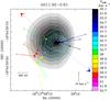 |
Fig. 2 Gray-scale image: JVLA A-Array C-band continuum, using gray-tone steps that increase linearly with the map intensity from 0.055 to 0.18 mJy beam-1. The JVLA A-Array Ku-band continuum is represented with cyan contours with plotted levels −30% and from 30% to 90%, in steps of 10%, of the peak value of 0.19 mJy beam-1. The white contours reproduce the JVLA A-Array K-band continuum, plotting levels −30% and from 30% to 90%, in steps of 10%, of the peak value of 0.27 mJy beam-1. Colored dots and arrows have the same meaning as in Fig. 1. The amplitude scale for the maser velocity is indicated by the black arrow in the bottom right of the panel. The red and blue arrows indicate the direction of the red- and blue-shifted lobes, respectively, of the bipolar collimated outflow observed in the 12CO(2–1) line using the SMA by Cyganowski et al. (2011). |
For some targets, of the observed (6–9) epochs spanning about one year, we selected the three or four epochs with the shortest time separations (spanning ≤5 months, see Tables A.1–A.11), over which many of the short-lived maser features could be measured. Maser spot positions were determined by fitting elliptical Gaussian brightness distributions. For a description of the criteria used to identify individual masing clouds, to derive their parameters (position, intensity, flux, and size) and to measure their (relative and absolute) proper motions, see the paper on VLBI observations of water and methanol masers by Sanna et al. (2010a).
The derived absolute water maser proper motions were corrected for the
apparent proper motion due to the Earth’s orbit around the Sun (parallax), the solar
motion and the differential Galactic rotation between our LSR and that of the maser
source. We have adopted a flat Galaxy rotation curve (R0 = 8.33 ± 0.16
kpc, Θ0 = 243 ± 6
km s-1; Reid et al. 2014), and the solar motion
( ,
,  , and
, and
 km s-1) by Schönrich et al. (2010), who recently revised the Hipparcos
satellite results. The adopted values for Galactic rotation and solar motion were
derived by fitting the data (parallaxes and proper motions) of 80 BeSSeL maser targets
(Reid et al. 2014, fit labelled “B1” in Table 4),
employing the Schönrich et al. values as priors for the solar motion.
km s-1) by Schönrich et al. (2010), who recently revised the Hipparcos
satellite results. The adopted values for Galactic rotation and solar motion were
derived by fitting the data (parallaxes and proper motions) of 80 BeSSeL maser targets
(Reid et al. 2014, fit labelled “B1” in Table 4),
employing the Schönrich et al. values as priors for the solar motion.
4.2. Bolometric luminosity estimate
We used archival infrared data to determine the bolometric luminosity for the sources in our sample. For sources with | b | < 1°, we used the Hi-GAL database (Molinari et al. 2010). For the remaining sources, luminosities were estimated using integrated fluxes from images extracted from online catalogs of mid-infrared surveys (WISE, Wright et al. 2010 and MSX, Egan et al. 2003) and point-source fluxes from far-infrared (IRAS, Neugebauer et al. 1984 and SCUBA, Di Francesco et al. 2008) online catalogs. Source luminosities were derived directly by integrating the area under the spectral energy distribution (SED) curves. Examination of the WISE and MSX images show that the mid-infrared emission for most of our sources (over a region of ±1′) appear to be dominated by a single YSO, which should also account for most of the far-infrared (IRAS) fluxes. Therefore, for most of the sources lacking Hi-GAL observations, we believe that the luminosities derived using the IRAS fluxes exceed the true values only by a factor of a few. The IRAS luminosities that, owing to multiple sources, might overestimate the luminosity from the YSO associated with the masers by up to an order of magnitude are bracketed in Table 1.
5. Results
5.1. Water maser and radio continuum
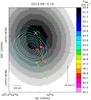 |
Fig. 3 Gray-scale image: JVLA A-Array C-band continuum, using gray-tone steps that increase linearly with the map intensity from 0.1 to 0.35 mJy beam-1. The JVLA A-Array Ku-band continuum is represented with cyan contours with plotted levels −20% and from 20% to 90%, in steps of 10%, of the peak value of 0.28 mJy beam-1. The white contours reproduce the JVLA A-Array K-band continuum, plotting levels −10% and from 10% to 90%, in steps of 10%, of the peak value of 0.55 mJy beam-1. Colored dots and arrows have the same meaning as in Fig. 1. The amplitude scale for the maser velocity is indicated by the black arrow in the bottom right of the panel. The white cross gives the (velocity-averaged) position of the 6.7 GHz methanol masers, detected at low velocity resolution in the C-band. |
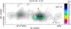 |
Fig. 4 Gray-scale image: JVLA A-Array C-band continuum, using gray-tone steps that increase linearly with the map intensity from 0.017 to 0.17 mJy beam-1. The JVLA A-Array Ku-band continuum is represented with cyan contours with plotted levels −20% and from 20% to 90%, in steps of 10%, of the peak value of 0.10 mJy beam-1. The white contours reproduce the JVLA A-Array K-band continuum, plotting levels −20% and from 20% to 90%, in steps of 10%, of the peak value of 0.28 mJy beam-1. Colored dots and arrows have the same meaning as in Fig. 1. The amplitude scale for the water maser velocity is indicated by the black arrow in the bottom right of the panel. The colored triangles denote the positions of the 6.7 GHz methanol masers, derived with the European VLBI Network by Sanna et al. (2010a). |
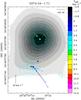 |
Fig. 5 Gray-scale image: JVLA A-Array C-band continuum, using gray-tone steps that increase linearly with the map intensity from 0.016 to 0.16 mJy beam-1. The JVLA A-Array Ku-band continuum is represented with cyan contours with plotted levels −10% and from 10% to 90%, in steps of 10%, of the peak value of 0.20 mJy beam-1. This source was not observed in the K-band by the JVLA. Colored dots and arrows have the same meaning as in Fig. 1. The amplitude scale for the maser velocity is indicated by the black arrow in the bottom left of the panel. |
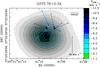 |
Fig. 6 Gray-scale image: JVLA A-Array C-band continuum, using gray-tone steps that increase linearly with the map intensity from 0.037 to 0.37 mJy beam-1. The JVLA A-Array Ku-band continuum is represented with cyan contours with plotted levels −10% and from 10% to 90%, in steps of 10%, of the peak value of 0.50 mJy beam-1. This source was not observed in the K-band by the JVLA. Colored dots and arrows have the same meaning as in Fig. 1. The amplitude scale for the maser velocity is indicated by the black arrow in the bottom right of the panel. The white cross gives the (velocity-averaged) position of the 6.7 GHz methanol masers, detected at low velocity resolution in C-band. |
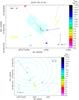 |
Fig. 7 Top panel: cyan contours: JVLA A-Array Ku-band continuum with plotted levels −10% and from 10% to 90%, in steps of 10%, of the peak value of 1.0 mJy beam-1. This source was not detected in our JVLA A-Array C-band observations, yelding a 5σ upper limit of ~70 μJy. This source was not observed in the K-band by the JVLA. Colored dots and arrows have the same meaning as in Fig. 1. The amplitude scale for the maser velocity is indicated by the black arrow in the bottom right of the panel. The black cross gives the (velocity-averaged) position of the 6.7 GHz methanol masers, detected at low velocity resolution in the C-band. The red and blue arrows indicate the direction of the red- and blueshifted lobes, respectively, of the bipolar collimated outflow observed in the 12CO(2–1) line by Sánchez-Monge (2011). The green dotted line gives the orientation of the elongated (Spitzer GLIMPSE 4.5 μm) “green fuzzy emission” detected in this region. Bottom panel: enlargement of the clustered water maser emission close to the Ku-band continuum peak. The cyan contours and the overlaid colored dots and arrows have the same meaning as in the top panel. The amplitude scale for the maser velocity is indicated by the black arrow in the bottom left of the panel. |
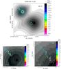 |
Fig. 8 Top panel: gray-scale image: JVLA A-Array C-band continuum, using gray-tone steps that increase linearly with the map intensity from 0.010 to 0.096 mJy beam-1. The JVLA A-Array Ku-band continuum is represented with cyan contours with plotted levels −10% and from 10% to 90%, in steps of 10%, of the peak value of 0.26 mJy beam-1. The white contours reproduce the JVLA A-Array K-band continuum, plotting levels −10% and from 10% to 90%, in steps of 10%, of the peak value of 0.5 mJy beam-1. Colored dots and arrows have the same meaning as in Fig. 1. Bottom panels: zoom on the area of the main, compact Ku- and K-band continuum sources (left) and on the water maser emission (right). In both panels, the gray-scale image, the cyan and white contours have the same meaning as in the top panel. Colored dots and arrows have the same meaning as in Fig. 1: for this clustered maser source, to better distinguish maser positions on top of the dark background, the colored dots are white-bordered. The amplitude scale for the maser velocity is indicated by the white arrow in the bottom left of the panels. |
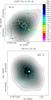 |
Fig. 9 Bottom panel: G097.53+3.18-Hii. The gray-scale image shows the JVLA A-Array (Gaussian-tapered) C-band continuum, using gray-tone steps that increase linearly with the map intensity from 0.46 to 4.6 mJy beam-1. The JVLA A-Array Ku-band continuum is represented with cyan contours with plotted levels −10% and from 10% to 90%, in steps of 10%, of the peak value of 0.54 mJy beam-1. The white contours reproduce the JVLA A-Array K-band continuum, plotting levels −20% and from 20% to 90%, in steps of 10%, of the peak value of 0.25 mJy beam-1. Top panel: G097.53+3.18-M. The gray-scale image shows the JVLA A-Array C-band continuum (produced selecting uv-projected lengths ≥100 kλ), using gray-tone steps that increase linearly with the map intensity from 0.014 to 0.14 mJy beam-1. The JVLA A-Array Ku-band continuum is represented with cyan contours with plotted levels −10% and from 10% to 90%, in steps of 10%, of the peak value of 0.16 mJy beam-1. The white contours reproduce the JVLA A-Array K-band continuum, plotting levels −20% and from 20% to 90%, in steps of 10%, of the peak value of 0.22 mJy beam-1. Colored dots and arrows have the same meaning as in Fig. 1. The amplitude scale for the maser velocity is indicated by the black arrow in the bottom left of the panel. |
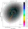 |
Fig. 10 Gray-scale image: JVLA A-Array C-band continuum, using gray-tone steps that increase linearly with the map intensity from 0.030 to 0.076 mJy beam-1. The JVLA A-Array Ku-band continuum is represented with cyan contours with plotted levels −20% and from 20% to 90%, in steps of 10%, of the peak value of 0.14 mJy beam-1. The white contours reproduce the JVLA A-Array K-band continuum, plotting levels −20% and from 20% to 90%, in steps of 10%, of the peak value of 0.22 mJy beam-1. Colored dots and arrows have the same meaning as in Fig. 1. The amplitude scale for the maser velocity is indicated by the black arrow in the bottom right of the panel. The black dashed line indicates the direction of the two nearby (separated by ~13′′), compact radio sources, detected at 3.6 cm with the VLA D-Array by Anglada & Rodríguez (2002). |
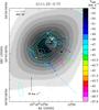 |
Fig. 11 Gray-scale image: JVLA A-Array C-band continuum, using gray-tone steps that increase linearly with the map intensity from 0.023 to 0.23 mJy beam-1. The JVLA A-Array Ku-band continuum is represented with cyan contours with plotted levels −10% and from 10% to 90%, in steps of 10%, of the peak value of 0.19 mJy beam-1. The white contours reproduce the JVLA A-Array K-band continuum, plotting levels −20% and from 20% to 90%, in steps of 10%, of the peak value of 0.22 mJy beam-1. Colored dots and arrows have the same meaning as in Fig. 1. The amplitude scale for the maser velocity is indicated by the black arrow in the bottom left of the panel. The white cross gives the (velocity-averaged) position of the 6.7 GHz methanol masers, detected at low velocity resolution in the C-band. |
This paper presents results for 11 high-mass YSOs. The continuum JVLA observations toward
G075.76+0.34 reveal another
nearby high-mass YSO, G075.78+0.34, which is also associated with a rich water maser cluster. Figures
1–11 present
the JVLA multiband continuum images overlaid on the water maser positions and proper
motions. Maser absolute positions are accurate within a few mas at their epoch of
observation. The apparent motions over the few years separating the maser VLBA (in
2009–2011) and the continuum JVLA (in 2012–2013) observations, are expected to be
≤10 mas. Thus, the
uncertainty on the absolute position of the continuum sources of 20–40 mas (see Sect.
3.1), should be the dominant source of error in the
alignment of the maser and the continuum images. For each target, the water masers and the
continuum emission are clearly associated. Typical flux densities for the continuum
sources were a few 100 μJy. Ku- and K-band emission consists of a single or a small
number of compact sources, and at least one of these sources is always found with a
separation ≤01
from the center of the water masers.
The C-band
continuum images show a variety of morphologies from compact (as, for instance, in
G012.68−0.18 and
G074.04−1.71), to slightly
resolved (in G111.25−0.77), to
elongated, jet-like (G016.58−0.05) and extended, quasi-spheroidal (G005.88−0.39 and G097.53+3.18) characteristics. Compact
C-band
components show a good positional correspondence with (within
01
from) Ku-
and/or K-band
peaks and the water masers. However, extended (a few arcseconds) C-band sources that are
partially or totally resolved out in Ku-band are typically offset by up to several
arcsec from the water masers. Table 3 lists the
parameters of all the continuum components detected within 5′′–10′′ of the water masers. These parameters
have been estimated by fitting an elliptical Gaussian brightness distribution to each
source of continuum emission. When multiple components are observed, the label number (#)
1 indicates the compact source, always detected at all the observed bands and associated
with the water masers.
Several of our targets are at low or high Dec (see Table 1), where the natural beam of the JVLA is elongated. We ran simulations of jets
(modeled as an elliptic object with varying sizes:
02
×
01,
04
×
02,
and 08
×
04)
to test the effects of the elongation of the beam on the continuum images that were
restored with a circular beam (see Table 2). We
simulated a 15 min, on-source observation at 15 GHz (corresponding to Ku-band) with the JVLA in
the A-Array configuration. We found that fitting an elliptical Gaussian brightness
distribution to images constructed with a round beam results in accurate size and position
angle (PA) estimates even if the dirty beam was elongated.
For each target, Tables A.1–A.11 list the fitted water maser intensity, VLSR, position, and proper motion for all detected features. Over the eleven sources, the number of maser features with measured proper motions ranges from a minimum of 9 (for G075.76+0.34) to a maximum of 26 (for G092.69+3.08 and G111.25−0.77). The average proper motion speed varies from source to source from 15 to 23 km s-1, with the exception of G016.58−0.05, with an average speed of 49 km s-1. Typical measurement errors are 3–5 km s-1, corresponding to relative uncertainties of ~20%.
A quantitative analysis of the geometrical and physical properties of the continuum emission and water maser flows is presented in Sect. 6. In the following we comment on the maser kinematics and continuum structure for each source, referring also to (sub-)arcsecond data in the literature that can be usefully compared with our measurements.
5.1.1. Comments on individual sources
1) G005.88-0.39.
The water maser emission is overlaid in projection on an extended (size ~45)
Hii region, intense (5 Jy) in the C-band, and resolved out by the JVLA A-Array in
the Ku-band
(see Fig. 1). Most of the water masers are
distributed and move on the sky along a direction that agrees well with that of the
collimated bipolar molecular outflow observed toward G005.88-0.39 on arcsecond scales
using the SMA by Sollins et al. (2004). It is
likely that the water masers are tracing the flow close to the YSO, which could coincide
with the near-infrared bright star revealed with VLT by Feldt et al. (2003) and placed near a cluster of strong maser spots (see inset
of Fig. 1). Since many of the detected water masers
project onto the extended Hii region, we argue that the YSO driving the
collimated molecular flow has to be located outside the ionized gas and is not the same
as the O-type star responsible for ionizing the Hii region.
2) G011.92 − 0.61.
The continuum emission in the C, Ku, and K-bands originates in a
compact source at the position of the water masers (see Fig. 2). The maser spatial distribution is compact (but slightly elongated
along the SE–NW), and most maser proper motions are directed toward the NE–SW, which
suggests that the masers trace an unresolved, NE–SW, collimated flow. Also, the
K-band
continuum is slightly elongated, with major axis oriented similarly to the maser proper
motions, possibly indicating an ionized jet. This conjecture is supported by the SMA
observations (HPBW =
24)
of Cyganowski et al. (2011), which in
correspondence with the water masers detect a compact hot core and a bipolar molecular
outflow (seen in the 12CO(2–1), HCO+(1–0), and SiO(2–1) line emissions) extending about
10′′ and tightly
collimated along a direction close to that of the maser velocities. The more compact
emission in the CH3CN and CH3OH lines presents a velocity gradient directed
perpendicular to the outflow axis, which may indicate rotation in an accretion disk. We
note that the proposed interpretation of the water maser velocity pattern in terms of an
outflow collimated NE–SW appears to contradict with the SE–NW elongated distribution of
the masers. The reasons for this different orientation can be investigated with
subarcsecond observations of the kinematics and physical conditions of the gas harboring
the water masers.
3) G012.68 − 0.18 (W33B).
The continuum structure and water maser kinematics are similar to those of the source G011.92−0.61 (see Fig. 3). At all frequency bands, a compact, slightly resolved continuum source is observed, which is aligned well in position with the main cluster of water masers. Water masers distribute over a few hundred au, and almost all the measured proper motions are directed toward the SW. Both the Ku- and K-band continuum emissions are slightly elongated and oriented like the maser proper motions. We tentatively interpret these observations in terms of an ionized jet and a collimated molecular flow traced by the radio continuum and water masers, respectively. This source is associated with a strong (peak flux density of ≥300 Jy) 6.7 GHz methanol maser, whose position, within the uncertainties of our JVLA A-Array C-band observations, coincides with the radio continuum peak at the center of the water maser distribution. The 6.7 GHz maser internal structure has been recently derived by Fujisawa et al. (2014). These authors find that the methanol masers trace an elongated structure, extended about 700 au along a SE–NW direction approximately perpendicular to the orientation of the water maser velocities. The observed regular variation of the 6.7 GHz maser VLSR with position could be consistent with Keplerian rotation in the envelope or disk surrounding a high-mass YSO. These 6.7 GHz VLBI observations provide indirect support for our interpretation of the continuum and water maser data in terms of an ionized and molecular collimated outflows, respectively.
4) G016.58 − 0.05.
This source is the best studied one in our sample, and its environment has been investigated recently at subarcsecond scales with JVLA B-Array NH3 observations (Moscadelli et al. 2013a). The (A-Array) C-band continuum emission is elongated by a few arcseconds in the E-W direction, marking an extended, ionized jet (see Fig. 4). This source is also associated with Spitzer Galactic Legacy Infrared Mid-Plane Survey Extraordinaire (GLIMPSE) 4.5 μm, “green fuzzy emission” (Cyganowski et al. 2008), possibly oriented in the same direction as the radio jet. Water masers are observed only on the western side of the jet and appear to trace a fast, wide-angle bow shock at the position where the jet interacts with denser material in the YSO’s surroundings. In the Ku and, particularly, the K-band, the continuum emission is relatively compact, dominated by an unresolved component placed at the center of the jet, where a cluster of 6.7 GHz methanol masers is also observed. The 3D velocities of the 6.7 GHz masers, measured with multi-epoch EVN observations (Sanna et al. 2010a), indicate that the masers could be in a rotating disk around a ~20 M⊙ YSO. In summary, our findings designate G016.58−0.05 as a clear example of a disk/jet system around an early-B–late-O type YSO.
5) G074.04 − 1.71.
The relatively low bolometric luminosity of this source (see Table 1) indicates that we are likely observing an intermediate-mass YSO. Both the C- and Ku-band continua consist of two compact sources connected by a bridge of lower intensity emission (see Fig. 5). The water maser distribution follows the continuum closely, drawing an arc of ~600 au in length. The maser proper motion vectors appear to rotate across the source and are locally directed approximately perpendicular to the maser arc and point outward, suggesting a global expansion from the arc center. Previous 12CO (3–2) line (HPBW = 22′′) observations by Mao et al. (2002) and H2 2 μm line imaging (angular resolution ~2′′) by Jiang et al. (2004) clearly identify an extended (size up to 100′′) outflow emerging from the position of the G074.04−1.71 YSO, whose structure (single vs multiple; collimated vs wide-angle) cannot, however, be confidently established using these data. No subarcsecond data are available in the literature for this source to be compared with our measurements.
6) G075.76 + 0.34.
The C- and Ku-band continuum emissions originate in a compact component, which is observed in the direction of a tight cluster (size ~300 au) of water masers (see Fig. 6). Maser velocities clearly trace a motion diverging from the center of the maser cluster with an average speed of ~10 km s-1. This source is associated with intense (peak flux density ~50 Jy, see Szymczak et al. 2012) 6.7 GHz maser emission, whose position, established with our JVLA A-Array C-band observations, agrees well with that of the water masers.
7) G075.78 + 0.34.
At a distance of 3.72±0.43 kpc, the inferred bolometric luminosity is 1.1 × 10⁴L⊙. Sánchez-Monge et al. (2013) have studied this star-forming region by means of subarcsecond VLA, Owens Valley Radio Observatory (OVRO), and SMA continuum and line observations. A clump of size ~0.1 pc harbors four radio continuum sources: 1) a cometary ultracompact (UC) Hii region with no associated dust emission; 2) an almost unresolved UC Hii region, located 6′′ to the E of the cometary UC Hii region and associated with a compact dust clump; 3) two compact sources embedded in a dust condensation of 30 M⊙, separated by 1400 au along NE–SW (PA = 45°) and placed 2′′ SW of the cometary arc. We have observed this region with the JVLA A-Array in the C and Ku-bands, detecting emission from the last two compact sources only in the Ku-band (see Fig. 7). The non detection in the C-band is consistent with the upper limit obtained by Sánchez-Monge et al. (2013) at the same frequency, while the differences in the Ku-band fluxes might be explained by the different sampling and resolution of the observations: Sánchez-Monge et al. (2013) used the VLA in the B and C configurations, sensitive to relatively extended emission and measuring a flux of 2 mJy, whereas in our observations with the A-Array, we filter out a fraction of this emission and detect only about 1 mJy. In the direction of the SW compact source, we observe a tight water maser cluster with a rather scattered pattern of proper motions. At larger separation (from a few hundred to a few thousand au) from this continuum component, water masers distribute along an almost straight line oriented SE–NW, with maser proper motions directed almost parallel to the maser line and heading away from the continuum source. Since independent outflow tracers (i.e., bipolar collimated (along PA ~ 30°) CO(2–1) and extended (at PA ~ 60°) IRAC 4.5 μm emissions (Sánchez-Monge et al. 2013, Fig. 7)) suggest the presence in this region of an outflow collimated along NE–SW, Sánchez-Monge et al. (2013) interpret the water maser pattern in terms of a wide-angle bow shock produced by the interaction of the jet/outflow with dense clump material. However, we note that the two nearby radio sources could be ionized by two distinct, high-mass YSOs, each emitting a massive, collimated outflow. Then, the CO(2–1) NE–SW outflow could be powered by the YSO ionizing the NE compact source, whereas the YSO at the position of the SW compact source could be driving a SE–NW collimated outflow, which can readily account for the highly elongated/collimated maser spatial/velocity distribution oriented SE–NW.
8) G092.69 + 3.08.
The C-band continuum emission of this source is extended, consisting of two adjacent resolved components separated by ~1′′ along the NE–SW direction (see Fig. 8). The strongest Ku- and K-band emissions come from an unresolved source at the position of the peak of the NE C-band component. Water masers present a NE–SW elongated distribution at radii from ~130 au to ~300 au from the Ku- and K-band source, and most of the maser proper motions are approximately parallel to the major axis of the maser spatial distribution and directed away from the compact continuum source. The simplest interpretation of the maser kinematics is in terms of a collimated outflow emerging from a YSO located at the position of the Ku- and K-band source. The extended C-band continuum, since it is elongated in the same direction of the water maser spatial and velocity distribution, could trace the ionized emission of the outflow lobe propagating to SW of the YSO. No interferometric data are available for this source in the literature.
9) G097.53 + 3.18.
The C-band
continuum image shows an extended (size ~34)
source, resolved out in the Ku and K-bands, where the emission is dominated by a
compact component at the position of the C-band peak (see Fig. 9, bottom panel). Water masers are not associated with this extended
source, but they cluster about 10′′ to the NE of it, where secondary C-, Ku-, and K-band components are
also detected (see Fig. 9, top panel). In the
following, we refer to the extended C-band source as G097.53+3.18-Hii and to the compact
radio source associated with the water masers as G097.53+3.18-M. In G097.53+3.18-M, the peaks of the C-, Ku-, and K-band components are
well aligned in position. While the C-band component is sligthly resolved along the
SE–NW direction, both the Ku- and K-band emissions are elongated toward NE–SW. Most
of the detected water masers are spread over the Ku- and K-band (elongated)
continuum, presenting a scattered pattern of proper motions. It is also interesting to
note that the Ku- and K-band emissions are more elongated toward the NE
than SW (with respect to the emission peak) and that the main cluster of water masers is
found to the SW of the emission peak. In G097.53+3.18-M, the asymmetrically elongated
continum, the concentration of water masers on the side of the shorter lobe, and the
wide-angle distribution of maser velocities, are somehow reminiscent of the case of the
radio jet in G016.58−0.05,
where the water maser emission likely originates in a wide-angle bow shock at the jet
head. Both the jet asymmetry and the water maser location might be a consequence of
density gradients in the surrounding environment, with higher densities resulting into a
reduced jet-lobe size and stronger water masing action. For this source, we found no
subarcsecond resolution interferometric data in the literature.
10) G100.38 − 3.58.
The continuum emission from all bands emerges from the same compact source (see Fig. 10), and water masers are observed toward this position, presenting a NE–SW elongated distribution spanning ~700 au. Proper motions are detected mainly for the features at the SW edge of the maser distribution, which appear to move away from the center of the maser cluster along directions forming a variety of angles (from low values up to ~90°) with respect to the cluster major axis. The (slightly resolved) K-band continuum (white contours in Fig. 10) is also elongated at similar PA as the water masers. Water masers are found between two compact radio sources (with fluxes of a few tenths of mJy) detected at 3.6 cm with the VLA D-Array by Anglada & Rodríguez (2002). The two compact sources are separated by ~13′′ along a direction (PA ~ 10°) approximately parallel to that of the water maser distribution. Based on this evidence, water masers might be tracing dense molecular material shocked and accelerated by the passage of a jet, whose ionized emission is traced near the YSO (at radii of ~103 au) by the JVLA A-Array C-, Ku-, and K-band continuum, and at larger separations (up to a few 104 au) by the VLA D-Array 3.6 cm emission. However, this interpretation faces some difficulties since it can explain neither the scattered pattern of maser proper motions nor the position of the radio continuum, which is actually offset (by a few 10 mas) to the W of the water maser linear distribution (see Fig. 10).
11) G111.25 − 0.77.
The C-,
Ku-, and
K-band
continuum emissions are well aligned in position and show a similar structure elongated
(by ~015)
in the SE–NW direction (see Fig. 11). In the
K-band
the emission is resolved in two distinct sources displaced SE–NW, with the NW source
being about three times more intense. Water masers show a rather scattered spatial
distribution covering all the Ku- and K-band emission region.
The maser proper motions, measured for many features, have orientations both parallel
and transverse to the direction of the continuum elongation, mainly tracing a receding
motion from the center of the Ku- and K-band continua. Toward
G111.25−0.77, Goddi et al. (2005) have measured the water maser
proper motions using the European VLBI Network (EVN), and the water maser emission and
associated radio continuum have been also observed with the VLA A-Array by Trinidad et al. (2006). These previous observations
are in good agreement with our BeSSeL/JVLA results, regarding the water maser kinematics
and the radio continuum structure.
5.2. Radio spectral index
Figures B.1–B.1 illustrate the method employed to derive the radio spectral index α (assuming Sν ∝ να, where Sν is the flux density at frequency ν) of the detected components. For each source, we used the images produced with identical pixels at the three observing frequencies and a uv-cutoff to limit both the lower and the higher frequency’s coverage. To take care of the small positional shifts between the components at different frequencies, we employed the following strategy:
-
1.
At each frequency, only emission peaks stronger than 3σ are considered.
-
2.
The emission region of each component is defined by the corresponding 3σ contour level.
-
3.
We name different components, i.e., emissions emerging at different positions, with “VLA 1”, “VLA 2”,..., “VLA n”, following the labeling of Table 3.
-
4.
At any given frequency, the flux of a component is computed using the 3σ contour levels defined in all the detection bands.
-
5.
If a component is not detected at a given frequency, the 3σ contour levels defined at the other frequency bands are used to compute upper limits of the flux.
For each target, Table 4 lists the fluxes determined as described above and the corresponding spectral indexes for each continuum component. When a component is detected in two or more frequency bands, the flux (or upper limit) reported at a given frequency is the weighted mean of the fluxes integrated over the 3σ polygons corresponding to the different detection bands, while the error is calculated as the dispersion of the weighted mean, and allows for a 10% error in the absolute flux scales. When fluxes (or upper limits) are available in all the three observing bands, the value of the spectral index is calculated over both the whole frequency interval of the observations, i.e., the [C–Ku–K] range, and the intermediate [C–Ku] and [Ku–K] ranges.
Coordinates, fluxes and sizes of the continuum sources detected with the JVLA.
6. Discussion
Our high angular resolution data allow us to infer the geometrical and physical properties of the outflows emitted by individual high-mass YSOs. In the following, we describe the methods employed to determine the outflow parameters and discuss the nature of the radio continuum emission.
6.1. Maser and radio continuum parameters
To establish the degree of collimation of the observed outflows in a quantitative fashion, we have derived the main geometrical parameters of the maser spatial and velocity distribution and compared them with the radio continuum morphology. For each source, Table 5 gives:
-
The PA of the major axis of the maser spatial distribution and the dispersions of the maser positions along the major and minor axes. These parameters define the orientation and degree of alignment of the maser positions.
-
The PA of the average direction and the angular scatter of the water maser proper motions. The average proper motion direction is evaluated as the one that minimizes the rms angular separation, Δθ, of the proper motions. In turn, Δθ can be taken as a measure of the semi-opening angle of the maser flow.
-
The average value and the dispersion of projected distances of the masers from the YSO (the latter assumed to be at the position of the compact Ku and/or K continuum emission).
-
The PA of the radio continuum emission (evaluated at the observing band where the continuum is more elongated) and the angular scatter of maser positions as seen from the YSO. The latter quantity is calculated as the rms angular separation from the outflow axis of the position vectors of the water masers from the YSO. It provides an alternative way to estimate the semi-opening angle of the outflow when water masers present a scattered pattern of proper motions, and are likely to be tracing a wide-angle bow shock at the jet tip(s) rather than a collimated flow.
In the next section, these maser and continuum parameters are employed to discuss the YSO’s outflow structure.
6.2. Outflow structure
Based on the spatial and velocity distribution of the water masers, the morphology of the radio continuum, and for some sources, the contribution of previous interferometric observations, we can divide our targets into two groups: 1) evidence of a collimated outflow; 2) lack of a clear-cut indication of a collimated outflow.
6.2.1. Group 1: collimated outflow
We have identified collimated outflows based on three different types of observational evidence:
Water masers. In two sources (G005.88−0.39, G092.69+3.08), the proper motions of the water masers are on average oriented close to the axis of the maser distribution. In G005.88−0.39, the positions and proper motions of most maser features are consistent with the direction of the bipolar collimated outflow revealed with the SMA on arcsecond scales (see Fig. 1). In G092.69+3.08, the collimated outflow traced by the water masers emerges from the position of the compact radio continuum (see Fig. 8). In this case, the radio emission likely originates in the same jet responsible for driving the motion of the water masers (see Sect. 6.4).
Radio continuum morphology. In our sample there is one source, G016.58−0.05, where the radio continuum emission is highly elongated across ~1′′ (Fig. 4), clearly tracing an ionized jet. Water masers in this source are observed only at the western edge of the jet, showing proper motions scattered over a wide range of PA. The simplest interpretation (as already pointed out in Sect. 5.1.1) is that the water masers trace a fast, wide-angle bow shock where the jet interacts with dense local material.
Other sources in our sample show a resolved structure in their radio continuum emission (slightly elongated or double components), but the comparison with the pattern of water maser’s proper motions does not clearly support the ionized jet interpretation.
Water maser plus radio continuum. In two sources (G011.92−0.61 and G012.68−0.18), water masers show concordant directions of motion, which are approximately parallel to the major axis of the radio continuum emission. In G011.92−0.61, an interpretation of these observations in terms of an ionized jet traced by the radio continuum and water masers is supported by SMA observations of a very collimated, bipolar, molecular outflow that is oriented similarly as the maser proper motions.
Depending on the kind of observational evidence used to identify the collimated outflows, their parameters (orientation and opening angle, reported in boldface in Table 5) were derived from either the maser spatial/velocity distribution or the radio continuum geometry (following the analysis described in Sect. 6.1).
6.2.2. Group 2: undetermined outflow structure
In the remaining six targets, we could not establish the outflow geometry. In the following, we briefly describe their main properties.
G075.78+0.34. In this source, water maser positions and proper motions hint at a collimated flow along a direction at PA ~ 100°–109° E of N (see Table 5), whereas the two nearby compact sources observed in the Ku-band (see Fig. 7), together with the bipolar CO(2–1) and extended IRAC 4.5 μm emissions detected on a larger angular scale, suggest an outflow collimated NE–SW, at PA ~ 45°. Following the analysis by Sánchez-Monge et al. (2013), the properties of the radio emission from the two compact sources are consistent with both homogeneous, hypercompact Hii regions and free-free radiation from a jet. Therefore, with the present data, it is difficult to decide if two distinct YSOs are driving two independent outflows collimated at different PAs or if the radio continuum and the water masers trace, respectively, ionized gas along the axis and an extended, wide-angle bow shock, generated by the same outflow.
G100.38−3.58. Looking at Table 5, this source is the one with the best collimated maser spatial distribution. However, as already pointed out in Sect. 5.1.1, the interpretation in terms of a collimated outflow is challenged by the misalignment of the maser proper motions (forming large angles with the axis of maser elongation) and by the position of the compact radio continuum (pinpointing the YSO), separated by a few 10 mas from the line of water masers.
G074.04−1.71, G097.53+3.18-M,
G111.25−0.77. These three sources share similar properties
for the maser kinematics and radio continuum geometry. In each of them, the structure of
continuum emission, observed in two or three bands, is elongated (size ~01–02),
even if not extended enough to be interpreted in terms of an ionized jet. Water masers
are projected on top of the elongated radio continuum and present a scattered pattern of
maser proper motions, since most are oriented at large angles from the major axis of the
continuum source.
G075.76+0.34. In this source, water masers trace a motion of expansion from the center of the maser cluster. Since, however, the peak of the Ku-band continuum, probably marking the location of the YSO, is offset toward the SE from the maser cluster by ≥50 mas (see Fig. 6), a simple interpretation of the water maser configuration in terms of a spherical, expanding flow might not hold in this case.
6.3. Outflow momentum
The momentum rate of the flow (reported for the collimated flows in the last column of
Table 5) was estimated from the water maser 3D
velocity distribution, assuming that all the momentum of the ejected (neutral or ionized)
jet is transferred to the surrounding molecular environment. Assuming that the position of
the YSO coincides with the peak of the Ku- and/or K-band continuum emission
(determined with an uncertainty of ~20 mas), the momentum rate Ṗ is calculated with the
formula (see Goddi et al. 2011):  (1)where V10 is the
average maser velocity in units of 10 km s-1, R100 is the average distance of water
masers from the YSO in units of 100 au, Ω the solid angle of the flow, and n8 the gas
volume density in units of 108 cm-3 (see, e.g., Moscadelli
et al. 2013b; Sanna et al. 2010b). A major
source of error comes from the uncertainty on the gas density, which, for most of our
sources, has been measured on much larger scales than those traced by the water masers.
However, by adopting n8 = 1, our estimate of Ṗ should be correct within
(at least) one order of magnitude, since excitation models constrain the density of the
shocked gas to be of ~108 cm-3 for strong maser action (Hollenbach et al. 2013). The
value of Ω is set to
4π and
2π(Δθ)2 for a
wide-angle and a collimated flow, respectively, where Δθ is the semi-opening
angle of the flow. As discussed in Sect. 6.2, the
analysis of the radio continuum and maser observations in our small sample of eleven
targets has enabled us to clearly identify only one kind of outflow structure, i.e.,
collimated outflows. The semi-opening angle of the collimated outflow is estimated from
the angular scatter of the maser proper motions or the maser positions (as seen from the
YSO), depending on whether the source shows a collimated or a scattered pattern of proper
motions, respectively (see Sect. 6.1 and Table 5).
(1)where V10 is the
average maser velocity in units of 10 km s-1, R100 is the average distance of water
masers from the YSO in units of 100 au, Ω the solid angle of the flow, and n8 the gas
volume density in units of 108 cm-3 (see, e.g., Moscadelli
et al. 2013b; Sanna et al. 2010b). A major
source of error comes from the uncertainty on the gas density, which, for most of our
sources, has been measured on much larger scales than those traced by the water masers.
However, by adopting n8 = 1, our estimate of Ṗ should be correct within
(at least) one order of magnitude, since excitation models constrain the density of the
shocked gas to be of ~108 cm-3 for strong maser action (Hollenbach et al. 2013). The
value of Ω is set to
4π and
2π(Δθ)2 for a
wide-angle and a collimated flow, respectively, where Δθ is the semi-opening
angle of the flow. As discussed in Sect. 6.2, the
analysis of the radio continuum and maser observations in our small sample of eleven
targets has enabled us to clearly identify only one kind of outflow structure, i.e.,
collimated outflows. The semi-opening angle of the collimated outflow is estimated from
the angular scatter of the maser proper motions or the maser positions (as seen from the
YSO), depending on whether the source shows a collimated or a scattered pattern of proper
motions, respectively (see Sect. 6.1 and Table 5).
Looking at Table 5, the derived values of outflow momentum rate vary in the range 10-3 to 100M⊙ yr-1 km s-1. For the two sources G005.88−0.39 and G011.92−0.61, the momentum rate derived from the water masers can be compared with that of the molecular outflow observed at larger angular scales (~1′′–10′′) and collimated along the same direction of the water maser flow. The momentum rate of the associated molecular flow for G005.88−0.39 is 0.33 M⊙ yr-1 km s-1 (Acord et al. 1997) and when assuming a flow inclination angle (with the plane of the sky) ≤30°, is ≥10-2M⊙ yr-1 km s-1 for G011.92−0.61 (Cyganowski et al. 2011). After comparing with the values in Table 5, the good agreement (within a factor of a few) between the maser and molecular momentum rates supports our method of deriving the outflow momentum from the water maser velocity distributions. In general, our result is consistent with the finding of previous single-dish surveys in large samples and interferometric measurements on individual objects. High-mass protostellar outflows have orders-of-magnitude higher momentum rates than typically found in low-mass protostars.
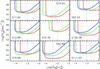 |
Fig. 12 Lyman continuum photon rate, NLy, versus Strömgren radius for all the compact sources of our sample. Each curve has been obtained by fixing the peak brightness temperature in the synthesized beam to the observed value. Red, green, and blue curves correspond, respectively, to the C-, Ku-, and K-band data. Pairs of curves are drawn to allow for 10% uncertainty on the measurements. The dotted vertical lines indicate the Hii regions radii estimated at the different frequencies with the same color coding as for the curves. The horizontal dotted lines indicate the value of NLy obtained from the bolometric luminosity, assuming that only one ZAMS star is ionizing the Hii region. This is to be considered an upper limit to the effective NLy. |
Spectral indexes and fluxes derived from the images created selecting the same uv-range across all the frequency bands.
The source G005.88−0.39 stands out for its extraordinarily high value of outflow momentum rate. In Sect 5.1.1, we have suggested that the high-mass YSO powering the massive molecular outflow resides outside the ionized gas and does not coincide with the O-type star exciting the Hii region. It is to be noted, however, that this is the only source where water masers are seen projected onto a relatively extended UC Hii region. This poses the question of whether a connection exists between the extreme value of outflow momentum rate and the UC Hii region. One could speculate, for instance, that the UC Hii region is close enough to the center of the massive outflow to accelerate it by radiation pressure. Future, subarcsecond-resolution observations that aim to study the outflow structure close to the UC Hii region have the potential to address this issue.
6.4. Nature of the radio continuum
Looking at Tables 3 and 4, one first notes that extended components are observed only in the
C-band
(with the exception of the elongated Ku-band component #2 in G016.58−0.05). In G005.88−0.39 and G097.53+3.18-Hii the approximately
spherical, extended (size of 3′′–5′′),
relatively intense (flux density ≥50 mJy), C-band emission traces an ultra-compact
Hii region, resolved out by the JVLA A-Array in the Ku-band. The much weaker
(with flux density in the range 0.1–0.5 mJy), extended C-band components observed
in the sources G016.58−0.05
and G092.69+3.08 are both
highly elongated and smaller than 13,
and their spectral indexes can be constrained with our JVLA observations. These extended
C-band
components are found to be offset from Ku- and K-band emission, and their spectral indexes are
negative, with values (or upper limits) varying in the range [−1.2, −0.3]. In particular, G016.58−0.05, which shows the clearest case for a
jet-like continuum morphology, presents a central component, probably placed close to the
YSO, with a steep (2.6 ± 0.3
in the [Ku–K] frequency range) spectral index, and elongated
components, which are offset from the YSO, prominent in the C-band, with a
[C–Ku] spectral index ≤−0.4. A similar change in the value of the spectral index with
position along the jet axis is also observed for the high-mass YSO’s HH80-81 jet (Carrasco-González et al. 2010). We interpret the
spatially resolved (at least in one direction) continuum detected only in the
C-band,
characterized by a negative value of the spectral index, in terms of synchrotron emission
from relativistic electrons accelerated in strong shocks produced by the protostellar jet.
So far, only a few non-thermal jets associated with high-mass YSOs have been observed. A
notable example is that of the luminous (105L⊙) Turner-Welch source in the W3(OH)
region, where multifrequency VLA observations have shown that the radio continuum is
highly elongated and has a negative spectral index α = −0.6 (Reid et al.
1995). With the caveat of the small sample, our detection of synchrotron emission from two
(G016.58−0.05 and
G092.69+3.08) out of the
eleven targets suggests that non-thermal emission could be common in high-mass
protostellar jets.
In all sources, the YSO is likely to be found close to the main compact component of the
radio continuum (labeled # 1 in Table 3), which is
always detected at all the observed bands (except for the non-detection in C-band in
G075.78+0.34). Water masers
are invariably distributed within ≤01
from this compact continuum emission, and in most cases the maser proper motions clearly
indicate that a molecular outflow is emerging from a position consistent with that of the
radio continuum. Our finding is consistent with previous observations of the few known
jets from high-mass YSO, where the YSO position is coincident with compact sources
detected from the radio to the near-infrared (see, e.g., the case of the massive jet in
AFGL5129, Johnston et al. 2013).
We first tried to fit the compact radio emission in terms of a homogeneous Hii region. Figure 12 shows that, when the emission has been observed at three frequencies, a consistent solution is never found, and solutions involving only two frequencies require a size for the Hii region that is significantly smaller than observed. We are thus prompted to conclude that these compact sources cannot be hyper- or ultra-compact Hii regions, unless the ionized gas harbors strong density (and likely velocity) gradients.
An examination of the measured spectral indexes (see Table 4) can help us to further constrain the nature of these compact continuum components. Interestingly, when the main component is detected in all the three observing bands, the [C–Ku] spectral index is systematically lower (or much lower) than the [Ku–K] spectral index. This effect is also evident when looking at the plots of the flux density distributions (see Figs. B.1–B.1), which show that the slope of the line connecting the C- and Ku-band fluxes is in general shallower than for the line connecting the Ku- and K-band fluxes. Our method of determining the fluxes for calculating the spectral index, by using images that are produced selecting the same uv-range and integrating over the same emission regions (≥3σ) across the three observing bands, should minimize the bias of both the increasing angular resolution and the varying source size with frequency.
The contribution of dust emission, stronger at higher frequencies, could in principle steepen the spectral index over the [Ku–K] frequency range. The intensity Iν of (optically thin) dust emission at frequency ν can be calculated with the expression Iν = Bν(T) κ(ν) Σ, where Bν(T) is the Planck function evaluated at the dust temperature T, κ(ν) = κ0(ν/ν0)β is the dust emission coefficient, and Σ the mass surface density of the star-forming core. Taking κ0 = 0.01 cm2 g-1 at ν0 = 230.6 GHz (Ossenkopf & Henning 1994), β = 1 (i.e., assuming a very mild frequency dependence of the dust emission) and an upper limit for the dust temperature T ≤ 300 K, to obtain an intensity in the K-band that is comparable to the measured values of the continuum emission of ~10-2 Jy arcsec-2, we derive a lower limit for the mass surface density Σ ≥ 100 g cm-2. This value is exceedingly high compared with the measurements in star-forming regions, which typically have 0.1 g cm-2 ≤ Σ ≤ 10 g cm-2 (see, e.g., Tan et al. 2014, Fig. 1). Thus, we consider it unlikely that dust emission causes the observed difference in spectral index between the [C–Ku] and [Ku–K] frequency ranges.
Geometrical parameters of the radio continuum and water masers.
The change in the slope of the spectrum between the [C–Ku] and [Ku–K] frequency ranges could be explained if the radio continuum from these compact components resulted from a combination of thermal (free-free) and non-thermal (synchrotron) emissions. In the C-band, for most of our sources, we might lack the angular resolution to spatially separate the contributions of the two physical processes near the YSO position. In this regard, it is very instructive to consider the case of the compact component #1 in G016.58−0.05, which is blended with the non-thermal component #2 in the C-band image at lower resolution (produced without applying a low uv cutoff; see Table 3), while, in the higher resolution C-band image used to determine the spectral index, it has the same position as the unresolved component #1 in the Ku and K-bands. To investigate the possibility that non-thermal emission contributes to the C-band flux, we redid the C-band (spectral index) images by averaging only the first four (centered at 5.50 GHz) and the last four (centered at 6.98 GHz) of the available sixteen IF sub-bands and determined the two-point spectral index over the C-band. Table 6 reports the fluxes at 5.50 and 6.98 GHz and the derived C-band spectral indexes. With the caveat that the reduced S/N of the two images (by using only one fourth of the total band) limits the precision of the spectral index (estimated errors of ~0.7), we find both negative and positive values, which vary in the interval [−1.8, 1.1]. For the source G092.69+3.08, the derived C-band spectral index, ~1, is in good agreement with both the [C–Ku] and the [Ku–K] values (see Table 4), nicely confirming the thermal nature of the emission of the main compact component observed close to the water masers. We note that G012.68−0.18 and G100.38−3.58, which are among the sources with the largest difference between the [Ku–K] and [C–Ku] spectral indexes (see Table 4), show the most negative values, ≲−1, of the C-band spectral index. That supports our conjecture that the C-band emission of these targets can be contaminated, or even dominated, by a non-thermal component. For G100.38−3.58, we also observe a change in the emission structure between 5.50 and 6.98 GHz. The structure is more extended and oriented at similar PA (~18°, see Fig. 10 and Table 5) as the water maser distribution at 5.50 GHz and more compact and elongated approximately perpendicular to the water maser pattern at 6.98 GHz. Here, we could actually be witnessing the change in the emission mechanism of the radio continuum across the frequency range of the C-band, from synchrotron emission, tracing the jet at the lower edge of the C-band, to thermal radiation from an ionized wind (observed nearby the YSO), at the upper edge of the C-band.
On the other hand, because of the higher frequency and angular resolution and their good positional correspondence, the Ku- and K-band continuum emissions should not be contaminated by non-thermal emission and reliably trace the same source of thermal radiation. Therefore, to determine the nature of the thermal emission, we prefer to rely on the value of the spectral index evaluated in the [Ku–K] frequency range. We note that four sources (G011.92−0.61, G075.78+0.34, G097.53+3.18-M, and G111.25−0.77) present a [Ku–K] spectral index that is consistent with the value, α = 0.6, expected for a spherical, isothermal, constant-velocity, ionized wind (Panagia & Felli 1975). The remaining four targets for which the [Ku–K] spectral index has been determined have values in the range 1.3–2.6, significantly more than 0.6. The calculations by Reynolds (1986) indicate that a conical, accelerating and/or recombining, ionized wind can have values of α ≥ 1. Actually, in three (G012.68−0.18, G016.58−0.05, and G092.69+3.08) of the four targets with a relatively high value of the [Ku–K] spectral index, the interpretation of the compact Ku- and K-band radio continuum in terms of an unresolved, collimated (conical) ionized wind is perfectly consistent with the elongated C-band continuum emission or the spatial/velocity pattern of water masers, which appear to trace a collimated flow as well. To conclude, we generally interpret the compact continuum emission spatially associated with the water masers in terms of an ionized wind, whose structure (wide-angle vs. collimated, constant-velocity vs accelerated) can vary from source to source.
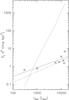 |
Fig. 13 Radio continuum specific luminosity (expressed by the product of the radio flux and the square of the distance) versus the bolometric luminosity (reported in Table 1). To produce this plot we have excluded the sources G075.78+0.34 and G097.53+3.18, since the derived bolometric luminosity is probably dominated by the hyper-compact or UC Hii region observed nearby the high-mass YSO associated with the water masers. The continuous line represents the best linear fit of the logarithm of the radio and the bolometric luminosities, the dashed line gives the relation between radio and bolometric luminosities observed in low-mass YSOs (Anglada et al. 2015), and the dotted line indicates the radio luminosities expected from the Lyman continua obtained from the bolometric luminosities. |
6.5. Comparison of the radio and bolometric luminosity
Despite the small number of sources analyzed, we have attempted an analysis of the statistical behavior of some relevant measurements. Figure 13 compares the radio (specific) luminosities of our sources with the bolometric luminosities. For producing this plot, we used the Ku-band radio flux (given in Table 3) available for all the sources in our sample except G005.88−0.39. Figure 13 indicates that a certain degree of correlation exists between the radio and the bolometric luminosities, a linear regression of the logarithm of these two quantities yelding a correlation coefficient of 0.82. The fitted power-law relation, Sνd2 [mJy kpc-2] = 0.21 (Lbol/L⊙)0.5, compared with the one derived for jets in low-mass YSOs, Sνd2 [mJy kpc-2] = 0.008 (Lbol/L⊙)0.6 (Anglada et al. 2015), has a similar power-law exponent, but a significantly larger scale factor. We warn that the derived relation is only based on eight sources, and it has to be tested using the full target sample.
Spectral indexes and fluxes in the C-band regime.
The fits of the Hii regions reported in Fig. 12 show that the Lyman continua derived from bolometric luminosities always exceed those obtained from the radio luminosities (except for the source G092.69+3.08). Accordingly, Fig. 13 shows that the radio luminosities inferred from the bolometric luminosities are much higher than the observed values. We now examine various explanations for this finding. First, we note that three sources (G011.92−0.61, G012.68−0.18, and G092.69+3.08) out of the four for which a reliable measurement of both the radio luminosity and the outflow momentum rate is available could satisfy the relation momentum rate – radio luminosity expected for shock-ionized, thermal jets (Rodríguez et al. 2008; Anglada 1996). When using the revised expression of the relation by Anglada et al. (2015) and the observed radio luminosities, the predicted momentum rates differ from the observed values by only a factor of a few for these three sources. In the case of G016.58−0.05, instead, the observed momentum rate overwhelms the predicted value by more than two orders of magnitude, but as discussed in Sect. 6.4, the jet in this source may be non-thermal. If, for most of our targets, the ionization of the observed compact, continuum sources were due to shocks in a thermal jet, that could explain the low values of radio luminosities, but it would make the problem of the missing continuum radiation from photo-ionization (i.e., ionized directly from the energetic stellar photons) even more serious.
As predicted by recent massive star formation models (see, e.g., Krumholz et al. 2009), most of the stellar energetic photons could escape through a YSO outflow cavity, leaving only a small fraction of the Lyman continuum for ionizing the base of the jet and making it “visible” to us. The escaped photons could then be absorbed at larger radii from the YSO and produce a distribution of low-density, ionized material in the outflow cavity that is too extended and/or weak to be detected with our JVLA A-Array observations. In this case, even if the gas is photo-ionized, we would be able to recover only a minor fraction of the radio luminosity expected from the Lyman continuum. Sensitive JVLA B- or C-Array observations of our targets can help establish whether most of the radio continuum emission is actually distributed on larger angular scales.
Star formation models and observations suggest that massive YSOs should accrete mass at high rates on the order of 10-4–10-3M⊙ yr-1. For such high, mass-infall rates, the models of Keto (2003, 2007) predict that the Hii region could be quenched or trapped, with sizes that, depending on the local gas density, can be as small as a few au. The radio continuum emission of a trapped Hii region would be much lower than expected from optically thin Hii regions, and this could account for the low radio luminosities of our targets. Another possibility is that high-mass YSOs simply do not produce intense Lyman continuum radiation. The calculations by Hosokawa & Omukai (2009) demonstrate that a massive protostar accreting at a very high rate of ~10-3M⊙ yr-1 has a very large radius, up to ~100 R⊙. A large radius means a low effective temperature, and if this remains below about 30 000 K, then there will not be any significant Lyman continuum output from the star. From the measured momentum rates of the collimated outflows (see Table 5), and taking the average maser velocity of ~20 km s-1 (see Sect. 5), we can derive a rough estimate for the outflow mass rate of 10-4–10-2M⊙ yr-1. If, as predicted by the star formation models, only a small fraction of the accretion flow is deflected and ejected, it is then plausible that the observed high-mass YSOs are accreting at rates as high as ~10-3M⊙ yr-1, consistent with the swollen star scenario. These conjectures could be tested by measuring the mass infall rates on scales of 100–1000 au through millimeter interferometer observations of suitable (optically thin and thick), high-density molecular tracers.
7. Summary and conclusions
This work presents a survey of outflows from high-mass YSOs carried out with unprecedented
sensitivity and angular resolution, enabling us to probe spatial scales from tens to
thousands au, which are relevant to investigating the ejection and collimation mechanisms.
In particular, we combine multi-epoch VLBA observations of the 22 GHz water masers to
measure the 3D velocity distribution of the molecular component of the flow (at
milli-arcsecond angular resolution and with 1 km s-1 accuracy) and sensitive JVLA observations of the radio
continuum at different frequencies (6, 13, and 22 GHz) to image the ionized emission on
angular scales of a few 01.
This observational strategy enables us to differentiate the blending pattern of several
outflows from nearby high-mass YSOs (which generally form in crowded clusters) and to
determine the geometrical and physical properties of outflows from individual high-mass
YSOs. Our source sample consists of 40 high-mass YSOs, selected from water masers of the
BeSSeL survey. This paper reports the initial results based on a subset of eleven targets.
The main findings of this paper are listed below:
-
At the angular resolution of our observations (0
1–02),
the continuum emission at 13 and 22 GHz always has a compact structure, whose position
corresponds well with that of the water masers. The continuum emission at 6 GHz can
comprise both compact and extended components. Compact 6 GHz components are mostly
well aligned in position with the 13/22 GHz emission peaks. We propose that these
unresolved radio continuum emissions probably indicate the YSO location. In many cases
the water maser proper motions trace a flow emanating from the continuum peak,
suggesting outflow activity from the central YSO. -
The comparison of the radio continuum morphology and the water maser’s spatial and velocity distribution indicates that five out of the eleven high-mass YSOs emit a collimated (conical) outflow (with flow semi-opening angle varying in the range 10°–30°). In the remaining six sources, the relationship between the radio continuum and water maser velocity pattern is more complex, which makes it difficult to draw conclusions on the outflow structure. The compact continuum detected at the base of the water maser flows always shows a positive spectral index in the frequency range 13–22 GHz. The measured spectral indexes are either consistent with the value, α = 0.6, expected for a spherical, isothermal, constant-velocity, ionized wind, or they fall in the range 1 ≤ α ≤ 2.6, which can be interpreted in terms of a conical, accelerating and/or recombining, ionized wind.
-
We find that the Lyman continua derived from the source bolometric luminosities always exceed those obtained from the radio luminosities. Consequently, we consider an interpretation of the compact continuum components in terms of photo-ionized hyper-compact Hii regions less likely than collisionally excited protostellar winds.
-
Two of our targets show weak (flux of 0.1–0.5 mJy), highly elongated emission at 6 GHz. The elongated emission is always offset (from a few 0
1
up to a few arcseconds) from the Ku- and K-band peaks and the
water masers. These two targets show negative spectral indexes across the 6–22 GHz
frequency range, with values (or upper limits) in the range [−1.2, −0.3]. We interpret the latter in terms
of non-thermal synchrotron emission from relativistic electrons accelerated in strong
shocks associated with the protostellar jets. These two sources will be observed
shortly with the JVLA at K-band in the B configuration. The latter
observations, yelding a good match in the uv-coverage with the JVLA A-Array
C-band
observations presented in this paper, will allow us to measure the radio spectral
index of the two targets more accurately and to verify its negative value. -
We estimate the momentum rates of the observed, collimated outflows, whose measured values vary in the range 10-3–100M⊙ yr-1 km s-1. These values are among the highest reported in the literature, indicating that the unprecedented angular resolution of our measurements enables us to identify extremely powerful outflow activity on the scales of individual high-mass YSOs.
These first results suggest that collimated outflows or jets could be common in high-mass YSOs, as well as in low-mass YSOs. Furthermore, our measurements provide hints that magnetic fields could be important in the process of jet collimation, as is widely recognised in the low-mass star formation case. This good correspondence suggests that low- and high-mass stars may share the same general formation process. In a following paper, we will report on the analysis of the whole sample of 40 high-mass YSOs and present a more complete discussion on the implications of these observations on theories of high-mass star formation and jet collimation/acceleration.
8. Appendix A: Additional tables
22.2 GHz H2O maser parameters for G005.88−0.39.
22.2 GHz H2O maser parameters for G011.92−0.61.
22.2 GHz H2O maser parameters for G012.68−0.18.
22.2 GHz H2O maser parameters for G016.58−0.05.
22.2 GHz H2O maser parameters for G074.04−1.71.
22.2 GHz H2O maser parameters for G075.76+0.34.
22.2 GHz H2O maser parameters for G075.78+0.34.
22.2 GHz H2O maser parameters for G092.69+3.08.
22.2 GHz H2O maser parameters for G097.53+3.18.
22.2 GHz H2O maser parameters for G100.38−3.58.
22.2 GHz H2O maser parameters for G111.25−0.77.
9. Appendix B: Additional figures
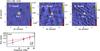 |
Fig. B.1 Upper panels: continuum images at the observed frequencies, from C to K-band moving from left to right. The target to which images and plots refer is indicated in the upper left of the figure. Images at different frequencies are reconstructed using a common, reduced uv-coverage, as described in Sect. 3.1. The field of view is centered on the observed (water maser) position reported in Table 2. In each image, the detected components are marked with polygons at the 3σ contour level, and if multiple components are observed, the corresponding polygons are labeled with increasing integer numbers. Lower plots: flux density distribution for each detected component. Red, green and blue colors indicate whether the fluxes have been computed from a polygon defined in the C-band, Ku-band, or K-band image, respectively. At a given frequency, either a dot or an arrowis used to denote if the component has been effectively detected at that particular frequency band or if the derived flux is only an upper limit. The solid line shows the linear fit performed over the whole observed frequency range, with the line color identifying the measurements considered to perform the fit. The fit slope, i.e., the spectral index, is indicated by the colored numbers reported in the lower right corner of the plot, with color denoting the corresponding linear fit. |
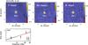 |
Fig. B.1 continued. |
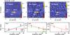 |
Fig. B.1 continued. |
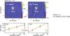 |
Fig. B.1 continued. |
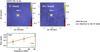 |
Fig. B.1 continued. |
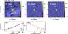 |
Fig. B.1 continued. |
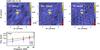 |
Fig. B.1 continued. |
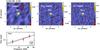 |
Fig. B.1 continued. |
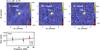 |
Fig. B.1 continued. |
NRAO is a facility of the National Science Foundation operated under cooperative agreement by Associated Universities, Inc.
An updated list of maser parallaxes can be found in Reid et al. (2014, see Table 1).
Acknowledgments
We are grateful to Rick Perley for the precious help in the calibration of the JVLA data. Á.S.-M. acknowledges support by the collaborative research center project SFB 956, funded by the Deutsche Forschungsgemeinschaft (DFG). A.S. gratefully acknowledges financial support by the Deutsche Forschungsgemeinschaft (DFG) Priority Program 1573. J.J. Li was supported by the National Science Foundation of China (Grants Nos. 11203082 and 11133008), the Natural Science Foundation of Jiangsu Province (Grants No. BK2012494), the Strategic Priority Research Program of the Chinese Academy of Sciences (Grants No. XDB09000000), and the Key Laboratory for Radio Astronomy, CAS.
References
- Acord, J. M., Walmsley, C. M., & Churchwell, E. 1997, ApJ, 475, 693 [NASA ADS] [CrossRef] [Google Scholar]
- Anglada, G. 1996, in Radio Emission from the Stars and the Sun, eds. A. R. Taylor, & J. M. Paredes, ASP Conf. Ser., 933 [Google Scholar]
- Anglada, G., & Rodríguez, L. F. 2002, Rev. Mex. Astron. Astrofis., 38, 13 [NASA ADS] [Google Scholar]
- Anglada, G., Rodriguez, L. F., & Carrasco-Gonzalez, C. 2015, Proc. Advancing Astrophysics with the Square Kilometre Array, PoS(AASKA14), 121 [Google Scholar]
- Arce, H. G., Shepherd, D., Gueth, F., et al. 2007, Protostars and Planets V, 245 [Google Scholar]
- Beltrán, M. T., Cesaroni, R., Moscadelli, L., & Codella, C. 2007, A&A, 471, L13 [NASA ADS] [CrossRef] [EDP Sciences] [Google Scholar]
- Beltrán, M. T., Cesaroni, R., Zhang, Q., et al. 2011, A&A, 532, A91 [CrossRef] [EDP Sciences] [Google Scholar]
- Beuther, H., & Shepherd, D. 2005, in Cores to Clusters: Star Formation with Next Generation Telescopes, eds. M. S. N. Kumar, M. Tafalla, & P. Caselli, 105 [Google Scholar]
- Beuther, H., Schilke, P., Sridharan, T. K., et al. 2002, A&A, 383, 892 [NASA ADS] [CrossRef] [EDP Sciences] [Google Scholar]
- Carrasco-González, C., Rodríguez, L. F., Anglada, G., et al. 2010, Science, 330, 1209 [NASA ADS] [CrossRef] [PubMed] [Google Scholar]
- Cesaroni, R., Felli, M., Jenness, T., et al. 1999, A&A, 345, 949 [NASA ADS] [Google Scholar]
- Choi, Y. K., Hachisuka, K., Reid, M. J., et al. 2014, ApJ, 790, 99 [NASA ADS] [CrossRef] [Google Scholar]
- Cunningham, A. J., Klein, R. I., Krumholz, M. R., & McKee, C. F. 2011, ApJ, 740, 107 [NASA ADS] [CrossRef] [Google Scholar]
- Curiel, S., Ho, P. T. P., Patel, N. A., et al. 2006, ApJ, 638, 878 [NASA ADS] [CrossRef] [Google Scholar]
- Cyganowski, C. J., Whitney, B. A., Holden, E., et al. 2008, AJ, 136, 2391 [NASA ADS] [CrossRef] [Google Scholar]
- Cyganowski, C. J., Brogan, C. L., Hunter, T. R., Churchwell, E., & Zhang, Q. 2011, ApJ, 729, 124 [NASA ADS] [CrossRef] [Google Scholar]
- Deller, A. T., Tingay, S. J., Bailes, M., & West, C. 2007, PASP, 119, 318 [NASA ADS] [CrossRef] [Google Scholar]
- de Villiers, H. M., Chrysostomou, A., Thompson, M. A., et al. 2015, MNRAS, 449, 119 [NASA ADS] [CrossRef] [Google Scholar]
- Di Francesco, J., Johnstone, D., Kirk, H., MacKenzie, T., & Ledwosinska, E. 2008, ApJS, 175, 277 [NASA ADS] [CrossRef] [Google Scholar]
- Egan, M. P., Price, S. D., & Kraemer, K. E. 2003, in AAS Meeting Abstracts, BAAS, 35, 1301 [NASA ADS] [Google Scholar]
- Feldt, M., Puga, E., Lenzen, R., et al. 2003, ApJ, 599, L91 [NASA ADS] [CrossRef] [Google Scholar]
- Fujisawa, K., Sugiyama, K., Motogi, K., et al. 2014, PASJ, 66, 31 [NASA ADS] [Google Scholar]
- Goddi, C., & Moscadelli, L. 2006, A&A, 447, 577 [NASA ADS] [CrossRef] [EDP Sciences] [Google Scholar]
- Goddi, C., Moscadelli, L., Alef, W., et al. 2005, A&A, 432, 161 [NASA ADS] [CrossRef] [EDP Sciences] [Google Scholar]
- Goddi, C., Moscadelli, L., & Sanna, A. 2011, A&A, 535, L8 [NASA ADS] [CrossRef] [EDP Sciences] [Google Scholar]
- Greenhill, L. J., Goddi, C., Chandler, C. J., Matthews, L. D., & Humphreys, E. M. L. 2013, ApJ, 770, L32 [NASA ADS] [CrossRef] [Google Scholar]
- Guzmán, A. E., Garay, G., & Brooks, K. J. 2010, ApJ, 725, 734 [NASA ADS] [CrossRef] [Google Scholar]
- Guzmán, A. E., Garay, G., Brooks, K. J., & Voronkov, M. A. 2012, ApJ, 753, 51 [NASA ADS] [CrossRef] [Google Scholar]
- Hosokawa, T., & Omukai, K. 2009, ApJ, 691, 823 [NASA ADS] [CrossRef] [Google Scholar]
- Immer, K., Reid, M. J., Menten, K. M., Brunthaler, A., & Dame, T. M. 2013, A&A, 553, A117 [NASA ADS] [CrossRef] [EDP Sciences] [Google Scholar]
- Jiang, Z.-B., Yang, J., Yao, Y.-G., Ishii, M., & Mao, R.-G. 2004, Chin. Astron. Astrophys., 28, 299 [NASA ADS] [CrossRef] [Google Scholar]
- Johnston, K. G., Shepherd, D. S., Robitaille, T. P., & Wood, K. 2013, A&A, 551, A43 [NASA ADS] [CrossRef] [EDP Sciences] [Google Scholar]
- Keto, E. 2003, ApJ, 599, 1196 [NASA ADS] [CrossRef] [Google Scholar]
- Keto, E. 2007, ApJ, 666, 976 [NASA ADS] [CrossRef] [Google Scholar]
- Kim, K.-T., & Kurtz, S. E. 2006, ApJ, 643, 978 [NASA ADS] [CrossRef] [Google Scholar]
- Krumholz, M. R., Klein, R. I., McKee, C. F., Offner, S. S. R., & Cunningham, A. J. 2009, Science, 323, 754 [NASA ADS] [CrossRef] [PubMed] [Google Scholar]
- Kuiper, R., Klahr, H., Beuther, H., & Henning, T. 2010, ApJ, 722, 1556 [CrossRef] [Google Scholar]
- Mao, R. Q., Yang, J., Henkel, C., & Jiang, Z. B. 2002, A&A, 389, 589 [NASA ADS] [CrossRef] [EDP Sciences] [Google Scholar]
- Marti, J., Rodríguez, L. F., & Reipurth, B. 1993, ApJ, 416, 208 [NASA ADS] [CrossRef] [Google Scholar]
- Marti, J., Rodríguez, L. F., & Reipurth, B. 1998, ApJ, 502, 337 [NASA ADS] [CrossRef] [Google Scholar]
- Matthews, L. D., Greenhill, L. J., Goddi, C., et al. 2010, ApJ, 708, 80 [NASA ADS] [CrossRef] [Google Scholar]
- Molinari, S., Swinyard, B., Bally, J., et al. 2010, PASP, 122, 314 [NASA ADS] [CrossRef] [Google Scholar]
- Moscadelli, L., Goddi, C., Cesaroni, R., Beltrán, M. T., & Furuya, R. S. 2007, A&A, 472, 867 [NASA ADS] [CrossRef] [EDP Sciences] [Google Scholar]
- Moscadelli, L., Cesaroni, R., Rioja, M. J., Dodson, R., & Reid, M. J. 2011, A&A, 526, A66 [NASA ADS] [CrossRef] [EDP Sciences] [Google Scholar]
- Moscadelli, L., Cesaroni, R., Sánchez-Monge, Á., et al. 2013a, A&A, 558, A145 [NASA ADS] [CrossRef] [EDP Sciences] [Google Scholar]
- Moscadelli, L., Li, J. J., Cesaroni, R., et al. 2013b, A&A, 549, A122 [NASA ADS] [CrossRef] [EDP Sciences] [Google Scholar]
- Neugebauer, G., Habing, H. J., van Duinen, R., et al. 1984, ApJ, 278, L1 [Google Scholar]
- Ossenkopf, V., & Henning, T. 1994, A&A, 291, 943 [NASA ADS] [Google Scholar]
- Panagia, N., & Felli, M. 1975, A&A, 39, 1 [NASA ADS] [Google Scholar]
- Reid, M. J., Menten, K. M., Brunthaler, A., et al. 2009, ApJ, 693, 397 [NASA ADS] [CrossRef] [Google Scholar]
- Reid, M. J., Menten, K. M., Brunthaler, A., et al. 2014, ApJ, 783, 130 [Google Scholar]
- Reynolds, S. P. 1986, ApJ, 304, 713 [NASA ADS] [CrossRef] [Google Scholar]
- Rodriguez, L. F. 1989, Rev. Mex. Astron. Astrofis., 18, 45 [NASA ADS] [Google Scholar]
- Rodríguez, L. F., Garay, G., Curiel, S., et al. 1994, ApJ, 430, L65 [NASA ADS] [CrossRef] [Google Scholar]
- Rodríguez, L. F., Moran, J. M., Franco-Hernández, R., et al. 2008, AJ, 135, 2370 [NASA ADS] [CrossRef] [Google Scholar]
- Sánchez-Monge, Á. 2011, Ph.D. Thesis, Universitat de Barcelona [Google Scholar]
- Sánchez-Monge, Á., Kurtz, S., Palau, A., et al. 2013, ApJ, 766, 114 [NASA ADS] [CrossRef] [Google Scholar]
- Sanna, A., Moscadelli, L., Cesaroni, R., et al. 2010a, A&A, 517, A71 [NASA ADS] [CrossRef] [EDP Sciences] [Google Scholar]
- Sanna, A., Moscadelli, L., Cesaroni, R., et al. 2010b, A&A, 517, A78 [NASA ADS] [CrossRef] [EDP Sciences] [Google Scholar]
- Sanna, A., Reid, M. J., Carrasco-González, C., et al. 2012, ApJ, 745, 191 [NASA ADS] [CrossRef] [Google Scholar]
- Sato, M., Wu, Y. W., Immer, K., et al. 2014, ApJ, 793, 72 [NASA ADS] [CrossRef] [Google Scholar]
- Schönrich, R., Binney, J., & Dehnen, W. 2010, MNRAS, 403, 1829 [NASA ADS] [CrossRef] [Google Scholar]
- Shepherd, D. S., Yu, K. C., Bally, J., & Testi, L. 2000, ApJ, 535, 833 [Google Scholar]
- Sollins, P. K., Hunter, T. R., Battat, J., et al. 2004, ApJ, 616, L35 [NASA ADS] [CrossRef] [Google Scholar]
- Surcis, G., Vlemmings, W. H. T., van Langevelde, H. J., et al. 2014, A&A, 565, L8 [NASA ADS] [CrossRef] [EDP Sciences] [Google Scholar]
- Szymczak, M., Wolak, P., Bartkiewicz, A., & Borkowski, K. M. 2012, Astron. Nachr., 333, 634 [NASA ADS] [CrossRef] [Google Scholar]
- Tan, J. C., Beltrán, M. T., Caselli, P., et al. 2014, Protostars and Planets VI, 149 [Google Scholar]
- Torrelles, J. M., Patel, N. A., Anglada, G., et al. 2003, ApJ, 598, L115 [NASA ADS] [CrossRef] [Google Scholar]
- Trinidad, M. A., Curiel, S., Torrelles, J. M., et al. 2006, AJ, 132, 1918 [NASA ADS] [CrossRef] [Google Scholar]
- Wolfire, M. G., & Cassinelli, J. P. 1987, ApJ, 319, 850 [NASA ADS] [CrossRef] [Google Scholar]
- Wright, E. L., Eisenhardt, P. R. M., Mainzer, A. K., et al. 2010, AJ, 140, 1868 [NASA ADS] [CrossRef] [Google Scholar]
- Wu, Y., Wei, Y., Zhao, M., et al. 2004, A&A, 426, 503 [NASA ADS] [CrossRef] [EDP Sciences] [Google Scholar]
- Xu, Y., Li, J. J., Reid, M. J., et al. 2013, ApJ, 769, 15 [NASA ADS] [CrossRef] [Google Scholar]
- Zhang, Q., Hunter, T. R., Brand, J., et al. 2005, ApJ, 625, 864 [NASA ADS] [CrossRef] [Google Scholar]
- Zhang, Q., Qiu, K., Girart, J. M., et al. 2014, ApJ, 792, 116 [NASA ADS] [CrossRef] [Google Scholar]
All Tables
Spectral indexes and fluxes derived from the images created selecting the same uv-range across all the frequency bands.
All Figures
|
Fig. 1 Gray-scale image and contours: JVLA A-Array C-band continuum, using gray-tone steps that increase linearly with the map intensity from 8 mJy beam-1 to the peak emission of 82 mJy beam-1, and contours corresponding to 10% to 90%, in steps of 10%, of the peak emission. The extended Ku-band emission is totally resolved out by our JVLA A-Array observations, and this source was not observed in the K-band by the JVLA. Colored dots show the absolute position of individual maser features, with color denoting the maser VLSR, according to the color-velocity conversion code reported on the right side of the panel. The green color gives the systemic VLSR, derived through (single-dish and/or interferometric) observations in high-density, thermal tracers. Dot area is proportional to the logarithm of the maser intensity. Colored arrows represent the measured maser proper motions, with dotted arrows used to represent the most uncertain proper motions. The amplitude scale for the maser velocity is indicated by the black arrow in the bottom right of the panel. The white errorbars denote the position (with the associated error) of the bright star detected in the near-infrared with the VLT by Feldt et al. (2003), and the red and blue arrows indicate the direction of the red- and blue-shifted lobes, respectively, of the bipolar collimated outflow observed in the SiO(5–4) line using the SMA by Sollins et al. (2004). The inset in the top right of the panel shows an enlargement of the clustered maser emission region close to the near-infrared star. |
| In the text | |
|
Fig. 2 Gray-scale image: JVLA A-Array C-band continuum, using gray-tone steps that increase linearly with the map intensity from 0.055 to 0.18 mJy beam-1. The JVLA A-Array Ku-band continuum is represented with cyan contours with plotted levels −30% and from 30% to 90%, in steps of 10%, of the peak value of 0.19 mJy beam-1. The white contours reproduce the JVLA A-Array K-band continuum, plotting levels −30% and from 30% to 90%, in steps of 10%, of the peak value of 0.27 mJy beam-1. Colored dots and arrows have the same meaning as in Fig. 1. The amplitude scale for the maser velocity is indicated by the black arrow in the bottom right of the panel. The red and blue arrows indicate the direction of the red- and blue-shifted lobes, respectively, of the bipolar collimated outflow observed in the 12CO(2–1) line using the SMA by Cyganowski et al. (2011). |
| In the text | |
|
Fig. 3 Gray-scale image: JVLA A-Array C-band continuum, using gray-tone steps that increase linearly with the map intensity from 0.1 to 0.35 mJy beam-1. The JVLA A-Array Ku-band continuum is represented with cyan contours with plotted levels −20% and from 20% to 90%, in steps of 10%, of the peak value of 0.28 mJy beam-1. The white contours reproduce the JVLA A-Array K-band continuum, plotting levels −10% and from 10% to 90%, in steps of 10%, of the peak value of 0.55 mJy beam-1. Colored dots and arrows have the same meaning as in Fig. 1. The amplitude scale for the maser velocity is indicated by the black arrow in the bottom right of the panel. The white cross gives the (velocity-averaged) position of the 6.7 GHz methanol masers, detected at low velocity resolution in the C-band. |
| In the text | |
|
Fig. 4 Gray-scale image: JVLA A-Array C-band continuum, using gray-tone steps that increase linearly with the map intensity from 0.017 to 0.17 mJy beam-1. The JVLA A-Array Ku-band continuum is represented with cyan contours with plotted levels −20% and from 20% to 90%, in steps of 10%, of the peak value of 0.10 mJy beam-1. The white contours reproduce the JVLA A-Array K-band continuum, plotting levels −20% and from 20% to 90%, in steps of 10%, of the peak value of 0.28 mJy beam-1. Colored dots and arrows have the same meaning as in Fig. 1. The amplitude scale for the water maser velocity is indicated by the black arrow in the bottom right of the panel. The colored triangles denote the positions of the 6.7 GHz methanol masers, derived with the European VLBI Network by Sanna et al. (2010a). |
| In the text | |
|
Fig. 5 Gray-scale image: JVLA A-Array C-band continuum, using gray-tone steps that increase linearly with the map intensity from 0.016 to 0.16 mJy beam-1. The JVLA A-Array Ku-band continuum is represented with cyan contours with plotted levels −10% and from 10% to 90%, in steps of 10%, of the peak value of 0.20 mJy beam-1. This source was not observed in the K-band by the JVLA. Colored dots and arrows have the same meaning as in Fig. 1. The amplitude scale for the maser velocity is indicated by the black arrow in the bottom left of the panel. |
| In the text | |
|
Fig. 6 Gray-scale image: JVLA A-Array C-band continuum, using gray-tone steps that increase linearly with the map intensity from 0.037 to 0.37 mJy beam-1. The JVLA A-Array Ku-band continuum is represented with cyan contours with plotted levels −10% and from 10% to 90%, in steps of 10%, of the peak value of 0.50 mJy beam-1. This source was not observed in the K-band by the JVLA. Colored dots and arrows have the same meaning as in Fig. 1. The amplitude scale for the maser velocity is indicated by the black arrow in the bottom right of the panel. The white cross gives the (velocity-averaged) position of the 6.7 GHz methanol masers, detected at low velocity resolution in C-band. |
| In the text | |
|
Fig. 7 Top panel: cyan contours: JVLA A-Array Ku-band continuum with plotted levels −10% and from 10% to 90%, in steps of 10%, of the peak value of 1.0 mJy beam-1. This source was not detected in our JVLA A-Array C-band observations, yelding a 5σ upper limit of ~70 μJy. This source was not observed in the K-band by the JVLA. Colored dots and arrows have the same meaning as in Fig. 1. The amplitude scale for the maser velocity is indicated by the black arrow in the bottom right of the panel. The black cross gives the (velocity-averaged) position of the 6.7 GHz methanol masers, detected at low velocity resolution in the C-band. The red and blue arrows indicate the direction of the red- and blueshifted lobes, respectively, of the bipolar collimated outflow observed in the 12CO(2–1) line by Sánchez-Monge (2011). The green dotted line gives the orientation of the elongated (Spitzer GLIMPSE 4.5 μm) “green fuzzy emission” detected in this region. Bottom panel: enlargement of the clustered water maser emission close to the Ku-band continuum peak. The cyan contours and the overlaid colored dots and arrows have the same meaning as in the top panel. The amplitude scale for the maser velocity is indicated by the black arrow in the bottom left of the panel. |
| In the text | |
|
Fig. 8 Top panel: gray-scale image: JVLA A-Array C-band continuum, using gray-tone steps that increase linearly with the map intensity from 0.010 to 0.096 mJy beam-1. The JVLA A-Array Ku-band continuum is represented with cyan contours with plotted levels −10% and from 10% to 90%, in steps of 10%, of the peak value of 0.26 mJy beam-1. The white contours reproduce the JVLA A-Array K-band continuum, plotting levels −10% and from 10% to 90%, in steps of 10%, of the peak value of 0.5 mJy beam-1. Colored dots and arrows have the same meaning as in Fig. 1. Bottom panels: zoom on the area of the main, compact Ku- and K-band continuum sources (left) and on the water maser emission (right). In both panels, the gray-scale image, the cyan and white contours have the same meaning as in the top panel. Colored dots and arrows have the same meaning as in Fig. 1: for this clustered maser source, to better distinguish maser positions on top of the dark background, the colored dots are white-bordered. The amplitude scale for the maser velocity is indicated by the white arrow in the bottom left of the panels. |
| In the text | |
|
Fig. 9 Bottom panel: G097.53+3.18-Hii. The gray-scale image shows the JVLA A-Array (Gaussian-tapered) C-band continuum, using gray-tone steps that increase linearly with the map intensity from 0.46 to 4.6 mJy beam-1. The JVLA A-Array Ku-band continuum is represented with cyan contours with plotted levels −10% and from 10% to 90%, in steps of 10%, of the peak value of 0.54 mJy beam-1. The white contours reproduce the JVLA A-Array K-band continuum, plotting levels −20% and from 20% to 90%, in steps of 10%, of the peak value of 0.25 mJy beam-1. Top panel: G097.53+3.18-M. The gray-scale image shows the JVLA A-Array C-band continuum (produced selecting uv-projected lengths ≥100 kλ), using gray-tone steps that increase linearly with the map intensity from 0.014 to 0.14 mJy beam-1. The JVLA A-Array Ku-band continuum is represented with cyan contours with plotted levels −10% and from 10% to 90%, in steps of 10%, of the peak value of 0.16 mJy beam-1. The white contours reproduce the JVLA A-Array K-band continuum, plotting levels −20% and from 20% to 90%, in steps of 10%, of the peak value of 0.22 mJy beam-1. Colored dots and arrows have the same meaning as in Fig. 1. The amplitude scale for the maser velocity is indicated by the black arrow in the bottom left of the panel. |
| In the text | |
|
Fig. 10 Gray-scale image: JVLA A-Array C-band continuum, using gray-tone steps that increase linearly with the map intensity from 0.030 to 0.076 mJy beam-1. The JVLA A-Array Ku-band continuum is represented with cyan contours with plotted levels −20% and from 20% to 90%, in steps of 10%, of the peak value of 0.14 mJy beam-1. The white contours reproduce the JVLA A-Array K-band continuum, plotting levels −20% and from 20% to 90%, in steps of 10%, of the peak value of 0.22 mJy beam-1. Colored dots and arrows have the same meaning as in Fig. 1. The amplitude scale for the maser velocity is indicated by the black arrow in the bottom right of the panel. The black dashed line indicates the direction of the two nearby (separated by ~13′′), compact radio sources, detected at 3.6 cm with the VLA D-Array by Anglada & Rodríguez (2002). |
| In the text | |
|
Fig. 11 Gray-scale image: JVLA A-Array C-band continuum, using gray-tone steps that increase linearly with the map intensity from 0.023 to 0.23 mJy beam-1. The JVLA A-Array Ku-band continuum is represented with cyan contours with plotted levels −10% and from 10% to 90%, in steps of 10%, of the peak value of 0.19 mJy beam-1. The white contours reproduce the JVLA A-Array K-band continuum, plotting levels −20% and from 20% to 90%, in steps of 10%, of the peak value of 0.22 mJy beam-1. Colored dots and arrows have the same meaning as in Fig. 1. The amplitude scale for the maser velocity is indicated by the black arrow in the bottom left of the panel. The white cross gives the (velocity-averaged) position of the 6.7 GHz methanol masers, detected at low velocity resolution in the C-band. |
| In the text | |
|
Fig. 12 Lyman continuum photon rate, NLy, versus Strömgren radius for all the compact sources of our sample. Each curve has been obtained by fixing the peak brightness temperature in the synthesized beam to the observed value. Red, green, and blue curves correspond, respectively, to the C-, Ku-, and K-band data. Pairs of curves are drawn to allow for 10% uncertainty on the measurements. The dotted vertical lines indicate the Hii regions radii estimated at the different frequencies with the same color coding as for the curves. The horizontal dotted lines indicate the value of NLy obtained from the bolometric luminosity, assuming that only one ZAMS star is ionizing the Hii region. This is to be considered an upper limit to the effective NLy. |
| In the text | |
|
Fig. 13 Radio continuum specific luminosity (expressed by the product of the radio flux and the square of the distance) versus the bolometric luminosity (reported in Table 1). To produce this plot we have excluded the sources G075.78+0.34 and G097.53+3.18, since the derived bolometric luminosity is probably dominated by the hyper-compact or UC Hii region observed nearby the high-mass YSO associated with the water masers. The continuous line represents the best linear fit of the logarithm of the radio and the bolometric luminosities, the dashed line gives the relation between radio and bolometric luminosities observed in low-mass YSOs (Anglada et al. 2015), and the dotted line indicates the radio luminosities expected from the Lyman continua obtained from the bolometric luminosities. |
| In the text | |
|
Fig. B.1 Upper panels: continuum images at the observed frequencies, from C to K-band moving from left to right. The target to which images and plots refer is indicated in the upper left of the figure. Images at different frequencies are reconstructed using a common, reduced uv-coverage, as described in Sect. 3.1. The field of view is centered on the observed (water maser) position reported in Table 2. In each image, the detected components are marked with polygons at the 3σ contour level, and if multiple components are observed, the corresponding polygons are labeled with increasing integer numbers. Lower plots: flux density distribution for each detected component. Red, green and blue colors indicate whether the fluxes have been computed from a polygon defined in the C-band, Ku-band, or K-band image, respectively. At a given frequency, either a dot or an arrowis used to denote if the component has been effectively detected at that particular frequency band or if the derived flux is only an upper limit. The solid line shows the linear fit performed over the whole observed frequency range, with the line color identifying the measurements considered to perform the fit. The fit slope, i.e., the spectral index, is indicated by the colored numbers reported in the lower right corner of the plot, with color denoting the corresponding linear fit. |
| In the text | |
|
Fig. B.1 continued. |
| In the text | |
|
Fig. B.1 continued. |
| In the text | |
|
Fig. B.1 continued. |
| In the text | |
|
Fig. B.1 continued. |
| In the text | |
|
Fig. B.1 continued. |
| In the text | |
|
Fig. B.1 continued. |
| In the text | |
|
Fig. B.1 continued. |
| In the text | |
|
Fig. B.1 continued. |
| In the text | |
Current usage metrics show cumulative count of Article Views (full-text article views including HTML views, PDF and ePub downloads, according to the available data) and Abstracts Views on Vision4Press platform.
Data correspond to usage on the plateform after 2015. The current usage metrics is available 48-96 hours after online publication and is updated daily on week days.
Initial download of the metrics may take a while.