| Issue |
A&A
Volume 581, September 2015
|
|
|---|---|---|
| Article Number | A124 | |
| Number of page(s) | 46 | |
| Section | Interstellar and circumstellar matter | |
| DOI | https://doi.org/10.1051/0004-6361/201526199 | |
| Published online | 21 September 2015 | |
Star and jet multiplicity in the high-mass star forming region IRAS 05137+3919 ⋆,⋆⋆
1
INAF, Osservatorio Astrofisico di Arcetri,
Largo E. Fermi 5, 50125
Firenze,
Italy
e-mail: This email address is being protected from spambots. You need JavaScript enabled to view it.
; This email address is being protected from spambots. You need JavaScript enabled to view it.
;
This email address is being protected from spambots. You need JavaScript enabled to view it.
; This email address is being protected from spambots. You need JavaScript enabled to view it.
;
This email address is being protected from spambots. You need JavaScript enabled to view it.
2
INAF, Osservatorio Astronomico di Bologna,
via Ranzani 1, 40127
Bologna,
Italy
e-mail: This email address is being protected from spambots. You need JavaScript enabled to view it.
3
INAF, Istituto di Astrofisica e Planetologia
Spaziale, Via Fosso del Cavaliere
100, 00133
Roma,
Italy
e-mail: This email address is being protected from spambots. You need JavaScript enabled to view it.
;
This email address is being protected from spambots. You need JavaScript enabled to view it.
4 Instituto de Astronomía, Universidad
Nacional Autónoma de México, Apdo.
Postal 877, Ensenada, B. C.,
CP 22830,
Mexico
e-mail: This email address is being protected from spambots. You need JavaScript enabled to view it.
5
European Southern Observatory, Karl-Schwarzschild-Str. 2, 85748
Garching,
Germany
e-mail: This email address is being protected from spambots. You need JavaScript enabled to view it.
6
INAF, Osservatorio Astronomico di Roma,
via di Frascati 33,
00040
Monte Porzio Catone,
Italy
e-mail: This email address is being protected from spambots. You need JavaScript enabled to view it.
7
Università degli Studi di Firenze, via Sansone 1, 50019
Sesto Fiorentino,
Italy
e-mail: This email address is being protected from spambots. You need JavaScript enabled to view it.
8
Steward Observatory, The University of Arizona,
933 N. Cherry Ave.,
Tucson, TX
85721,
USA
e-mail: This email address is being protected from spambots. You need JavaScript enabled to view it.
, This email address is being protected from spambots. You need JavaScript enabled to view it.
Received: 27 March 2015
Accepted: 16 July 2015
Abstract
Context. We present a study of the complex high-mass star forming region IRAS 05137+3919 (also known as Mol8), where multiple jets and a rich stellar cluster have been described in previous works.
Aims. Our goal is to determine the number of jets and shed light on their origin, and thus determine the nature of the young stars powering these jets. We also wish to analyse the stellar clusters by resolving the brightest group of stars.
Methods. The star forming region was observed in various tracers and the results were complemented with ancillary archival data. The new data represent a substantial improvement over previous studies both in resolution and frequency coverage. In particular, adaptive optics provides us with an angular resolution of 80 mas in the near IR, while new mid- and far-IR data allow us to sample the peak of the spectral energy distribution and thus reliably estimate the bolometric luminosity.
Results. Thanks to the near-IR continuum and millimetre line data we can determine the structure and velocity field of the bipolar jets and outflows in this star forming region. We also find that the stars are grouped into three clusters and the jets originate in the richest of these, whose luminosity is ~ 2.4 × 10⁴L⊙. Interestingly, our high-resolution near-IR images allow us to resolve one of the two brightest stars (A and B) of the cluster into a double source (A1+A2).
Conclusions. We confirm that there are two jets and establish that they are powered by B-type stars belonging to cluster C1. On this basis and on morphological and kinematical arguments, we conclude that the less extended jet is almost perpendicular to the line of sight and that it originates in the brightest star of the cluster, while the more extended one appears to be associated with the more extincted, double source A1+A2. We propose that this is not a binary system, but a small bipolar reflection nebula at the root of the large-scale jet, outlining a still undetected circumstellar disk. The gas kinematics on a scale of ~0.2 pc seems to support our hypothesis, because it appears to trace rotation about the axis of the associated jet.
Key words: stars: early-type / stars: formation / ISM: jets and outflows
Based on observations carried out with the Large Binocular Telescope. The LBT is an international collaboration among institutions in the United States, Italy and Germany. LBT Corporation partners are: The University of Arizona on behalf of the Arizona university system; Istituto Nazionale di Astrofisica, Italy; LBT Beteiligungsgesellschaft, Germany, representing the Max-Planck Society, the Astrophysical Institute Potsdam, and Heidelberg University; The Ohio State University, and The Research Corporation, on behalf of The University of Notre Dame, University of Minnesota, and University of Virginia.
Appendix A is available in electronic form at http://www.aanda.org
© ESO, 2015
1. Introduction
Observationally, the study of high-mass star formation is severely hindered by the difficulty of identifying the object of interest in a crowded region. This is basically the result of the large distances of OB-type stars (typically, several kpc) and the presence of numerous, lower mass stars in the same field. As a matter of fact, OB-type stars form in rich clusters, which makes it difficult to distinguish the phenomena associated with the high-mass star(s) of interest from those associated with other cluster members. High angular resolution is thus crucial for this type of investigation, since the (projected) separation inside these rich stellar cluster may be ≪1′′. Resolutions that high can be attained by IR and radio interferometers as well as by 8-m class telescopes operating at IR wavelengths, which are made possible through adaptive optics techniques.
With this in mind, we have focused our attention on a massive star forming region, where
evidence of multiple, young stellar objects (YSOs) was found. The corresponding counterpart
in the IRAS PSC is IRAS 05137+3919, also known as Mol 8 from the catalogue of Molinari et
al. (1996). These authors quote a kinematic distance
of 10.8 kpc and a corresponding luminosity (estimated from the IRAS fluxes) of
5.6 ×
104L⊙. Recently, Honma et al.
(2011) have measured the parallax of the water
masers in this object, resulting in a distance of
11.6 kpc. The same authors also establish a lower
limit of 8.3 kpc. This is consistent with a more recent parallax measurement by Reid et al.
(2014), who derive a distance of
7.7
kpc. The same authors also establish a lower
limit of 8.3 kpc. This is consistent with a more recent parallax measurement by Reid et al.
(2014), who derive a distance of
7.7 kpc, implying an uncertainty of a factor
~2 in luminosity. In the
following, we adopt the minimum distance of 8.3 kpc estimated by Honma et al. (2011), with the caveat that higher values are possible.
kpc, implying an uncertainty of a factor
~2 in luminosity. In the
following, we adopt the minimum distance of 8.3 kpc estimated by Honma et al. (2011), with the caveat that higher values are possible.
IRAS 05137+3919 does not satisfy the colour constraints established by Wood & Churchwell (1989) to identify (UC) Hii regions in the IRAS PSC, because the colour index [60–12] = 1.29 lies – although marginally – below the limit of 1.3. Indeed, despite the luminosity above 104L⊙, the source was not detected at 6 cm and 2 cm by Molinari et al. (1998), while only weak, compact continuum emission (0.33 mJy; Molinari et al. 2002) was measured at 3.6 cm. Whether this originates in an Hii region or in a thermal jet still needs to be understood, but it appears likely that the 3.6 cm continuum emission is associated with one of the members of the embedded stellar cluster detected in the near IR by various authors (Ishii et al. 1998; 2002; Varricat et al. 2010) and studied by Faustini et al. (2009), Kumar et al. (2006), and Nikoghosyan & Azatyan (2014; 2015). The most likely candidates for ionising the radio source are two bright stars located at the centre of the cluster and already identified by Varricat et al. (2010).
Interstingly, that cluster lies also close to the geometrical center of a bipolar outflow mapped in the 12CO(1–0) line by Zhang et al. (2001; 2005). Varricat et al. (2010) imaged two bipolar jets in the H2v = 1–0 S(1) line, also centred on the stellar cluster and directed approximately NE–SW and NW–SE. Hereafter, we refer to these, respectively, as Jet 1 and Jet 2, following Varricat et al. (2010). The former is roughly oriented like the 12CO outflow by Zhang et al. (2001; 2005) and the HCO+(1–0) outflow mapped by Molinari et al. (2002) with the OVRO interferometer. The presence of shocked H2 emission is confirmed by the near-IR spectra obtained by Ishii et al. (2001), which refer to the NW–SE jet.
Based on these previous findings, we decided to perform a multi-wavelength study of IRAS 05137+3919 with the main goal to relate the properties of the stellar cluster to those of the outflows/jets and hence identify the sources powering the flows and establish their nature. For these purposes, we obtained outflow maps a factor ~4 better in angular resolution than those by Zhang et al. (2005) and imaged the stellar cluster with an 8-m class telescope employing adaptive optics to attain ~0.̋08. We also used the continuum far-IR images of the Herschel/Hi-GAL survey (Molinari et al. 2010) to accurately estimate the cluster luminosity. After describing the observational details in Sect. 2, we illustrate the results in Sect. 3, while the analysis and discussion of our findings is presented in Sect. 4. Finally, the conclusions are drawn in Sect. 5.
2. Observations and data reduction
2.1. Large binocular telescope
2.1.1. Near-IR images with LUCI
Near-IR images were taken in the night of December 12, 2009 with LUCI (Seifert et al.
2003) at the Large Binocular Telescope (Mount
Graham, Arizona), through the standard broad-band filters H (λc =
1.653μm) and Ks (λc =
2.163μm), and the narrow-band filters FeII
(λc =
1.646μm, including the [FeII] 1.64-μm line) and
H2
(λc = 2.122
μm, including the H2v = 1–0 S(1) line at 2.12
μm). We
used the N3.75 camera with a pixel scale of ~ and a field of view of
4′× 4′. We took ten dithered images both at
H and at
Ks, each composed of 17 coadds of 2 s
exposures (H) and 15 coadds of 2 s exposures (Ks). A set of
14 dithered images, each resulting from coadding five exposures of 20 s, were taken at
H2, whereas
eight dithered images were taken at FeII, each of them a coadd of nine exposures of 20
s. Total exposure times were then 300 s (Ks), 340 s (H), 1400 s
(H2), and 1440
s (FeII), respectively. The dithering pattern consisted in alternatively imaging the
target in the central part, the eastern part, and the western part of the detector field
(i.e., with a throw of ~1′
in right ascension), with a random jitter of a few arcsec when the target was in the
same area of the detector. These allowed us to obtain sky images from the on-source
images themselves, by median filtering together 4 frames selected so that the target
area did not overlap in the stack, which would have been a problem due to the extended
emission feature in the field centre. All the images were flat-fielded, bad-pixel
corrected, sky-subtracted, registered, and combined by using standard IRAF1 routines. We note that, given the dithering strategy
adopted, all final combined images attain their maximum signal-to-noise ratio in a
central area ~2′
wide in right ascension. The full width at half maximum (FWHM) of the point-spread
function (PSF) was between ~
and a field of view of
4′× 4′. We took ten dithered images both at
H and at
Ks, each composed of 17 coadds of 2 s
exposures (H) and 15 coadds of 2 s exposures (Ks). A set of
14 dithered images, each resulting from coadding five exposures of 20 s, were taken at
H2, whereas
eight dithered images were taken at FeII, each of them a coadd of nine exposures of 20
s. Total exposure times were then 300 s (Ks), 340 s (H), 1400 s
(H2), and 1440
s (FeII), respectively. The dithering pattern consisted in alternatively imaging the
target in the central part, the eastern part, and the western part of the detector field
(i.e., with a throw of ~1′
in right ascension), with a random jitter of a few arcsec when the target was in the
same area of the detector. These allowed us to obtain sky images from the on-source
images themselves, by median filtering together 4 frames selected so that the target
area did not overlap in the stack, which would have been a problem due to the extended
emission feature in the field centre. All the images were flat-fielded, bad-pixel
corrected, sky-subtracted, registered, and combined by using standard IRAF1 routines. We note that, given the dithering strategy
adopted, all final combined images attain their maximum signal-to-noise ratio in a
central area ~2′
wide in right ascension. The full width at half maximum (FWHM) of the point-spread
function (PSF) was between ~ and ~
and ~ .
.
We scaled the Ks and H2 final mosaics appropriately
(by assuming a constant stellar continuum flux, which is correct only as a zero-order
approximation) and then subtracted one from the other, to obtain a continuum-free map of
pure H2 line
emission. In practice, we solved the two equations that give the intensities measured in
the H2 and
Ks filters
 with respect to
 and
and
 , where
 and
are the H2 line and continuum flux
densities, ΔνH2 and ΔνKs the
widths of the H2
and Ks filters, tH2
and tKs the
corresponding integration times, and ηH2 and ηKs the
transparencies of the two filters. We followed the same procedure with the
H and
FeII final mosaics, but no [FeII] emission could be detected in the subtracted image, so
we do not discuss the [FeII] data further.
and
are the H2 line and continuum flux
densities, ΔνH2 and ΔνKs the
widths of the H2
and Ks filters, tH2
and tKs the
corresponding integration times, and ηH2 and ηKs the
transparencies of the two filters. We followed the same procedure with the
H and
FeII final mosaics, but no [FeII] emission could be detected in the subtracted image, so
we do not discuss the [FeII] data further.
We performed PSF-fit photometry on the Ks and H final averaged (mosaiced) images by using the DAOPHOT routines in IRAF. In total, we found 1303 sources with detection at both Ks and H, 143 sources with detection at Ks and 60 sources with detection at H (see Table A.1). Unfortunately, the standard star observed for calibration during the night was saturated in all frames. Thus, we calibrated our photometry on 2MASS, by matching our sources to 2MASS PSC entries. For both bands, the colour range spanned by the common stars is too narrow to clearly show any colour effects between our instrumental magnitudes and 2MASS magnitudes, so we neglected colour terms. We obtained Ks(2MASS) − Ks(instrumental) = 23.81 ± 0.06 and H(2MASS) − H(instrumental) = 24.52 ± 0.05. The limiting magnitudes (at 3σ) are Ks ≃ 20 and H ≃ 20.5. A simple method of estimating the photometric completeness limits relies on histograms of magnitudes. Typically, the number of sources retrieved increases with increasing magnitudes up to a maximum value. Beyond this value, the source statistics is dominated by the decreasing efficiency in retrieving faint sources. Thus, the histogram maximum yields a rough estimate of the completeness limit. We conservatively assumed it to be 1 magnitude brighter than the histogram maximum. In fact, we found two nearby peaks at H, but the brighter one disappears when counting only sources in the 2′ innermost part of the image. So the brighter peak is probably due to including sources from parts of the image with lower signal-to-noise ratio. The completeness limits we estimated are Ks(compl) ~ 17.75 and H(compl) ≃ 18.25.
Finally, we calibrated the line emission fluxes on the final averaged (mosaiced) H2 image by repeating our photometry on the H2 image and matching it to the Ks calibrated photometry, correcting the stellar fluxes to the λc of the narrow-band filter. Photometry of the H2 knots was then performed on the continuum-subtracted H2 images by means of task POLYPHOT in IRAF, enclosing each knot with polygons following the emission contour at 3σ of the background counts as closely as possible. The identified knots and corresponding fluxes are given in Tables A.2 to A.4, where we have classified the knots on the basis of their association with Jet 1, Jet 2, and Jet 3 (defined in Sect. 3.3). For the H2 images the 3σ sensitivity level is equal to 4 × 10-16 erg s-1 cm-1 arcsec-2.
2.1.2. Near-IR images with FLAO and the PISCES camera
The data were collected on October 9 and 12, 2013, using the PISCES Near Infrared
Camera (McCarthy et al. 2001) installed at the
focal plane of the First Light Adaptive Optics system (Esposito et al. 2010, 2011) of
the Large Binocular Telescope. The detector has a pixel scale of ~ , with a field of view of
21′′× 21′′. The observations were carried out
through the H2,
H, and
Ks filters. We used a star
10′′ west from our field
center with R, I mag ~12.0 as the reference for the AO loop, closed using 153 modes.
The average Strehl Ratio on the centre of the field was 40% being measured on the
H2 images. The
electronic cross-talk between the quadrants in the PISCES Hawaii-I detector was
corrected for each frame using Corquad , an IRAF procedure developed by Roelof de
Jong2.
, with a field of view of
21′′× 21′′. The observations were carried out
through the H2,
H, and
Ks filters. We used a star
10′′ west from our field
center with R, I mag ~12.0 as the reference for the AO loop, closed using 153 modes.
The average Strehl Ratio on the centre of the field was 40% being measured on the
H2 images. The
electronic cross-talk between the quadrants in the PISCES Hawaii-I detector was
corrected for each frame using Corquad , an IRAF procedure developed by Roelof de
Jong2.
We obtained one image per band by registering and combining together, after sky
subtraction: 119 exposures of 5 s at Ks (total integration time 595 s); 62
exposures of 25 s at H2 (total integration time 1550 s); and 3 exposures of 10
s at H (30
s). Due to the deteriorating weather conditions, only the latter small set of
H frames
is available. Each single frame was first drizzled, bad-pixel corrected, and flat
fielded using standard IRAF routines. The PSF-FWHMs we measured are ~ in all final images.
We performed aperture photometry on the PISCES final images by using the DAOPHOT routines in IRAF. We found 66 sources with detection both at Ks and H, 83 sources with detection at Ks, and 24 sources with detection at H (see Table A.5). We used aperture radii of ~1 PSF-FWHM and annuli with inner and outer radii of ~2–4 PSF-FWHM to derive the sky level, with the median as an estimator. We calibrated Ks and H by comparing the instrumental magnitudes to those obtained with LUCI (which in turn are calibrated on 2MASS) for the matching stars. Again, the colour range spanned by the data points is too narrow to show any clear colour effects, so we neglected colour terms. We obtained Ks(LUCI, 2MASS) − Ks(PISCES, instrumental) = 23.46 ± 0.10 and H(LUCI, 2MASS) − H(PISCES, instrumental) = 24.68 ± 0.11. We note that a few points depart by up to 0.4 mag from these relations. The most extreme differences are clearly due to unresolved objects in the LUCI images. Nevertheless, part of the scatter is probably due to PSF variations over the PISCES field (anisoplanatism), which is typical of AO-assisted images (e.g., Esslinger & Edmunds 1998). So, we can actually expect intrinsic errors of up to 0.1–0.2 mag in our PISCES photometry. The limiting magnitudes (at 3σ) are Ks ≃ 22.5 and H ≃ 21. We estimated the completeness limits as explained in Sect. 2.1.1. The distribution of Ks displays two nearby peaks (see Sect. 4.1), but the brightest one is likely to be intrinsic to the local stellar population. Thus, we derived Ks(completeness) ≃19.25 and H(completeness) ≃ 18.75. Finally, from the Ks and H2 images we obtained a continuum-free, pure H2 line emission map following the method described in Sect. 2.1.1.
2.2. Ground based mid-IR observations
Ground-based diffraction-limited mid-infrared images at 8.9, 9.9, 12.7, and 18.7
μm of
IRAS 05137+3919 were taken on the night of November 9, 2006 with the mid-infrared camera
CID (Salas et al. 2006) mounted on the 2.1 m
telescope of the Observatorio Astronómico Nacional at San Pedro Mártir, Baja California,
Mexico. This camera is equipped with a Rockwell 128 × 128 square pixel Si:As BIB detector array that delivers an
effective scale of  covering a fully-sampled area
of 62′′× 62′′. The images were taken with the standard
chop-nodding mode to remove the sky and telescope emission background. The standard stars
α Lyr,
β And,
α Aur,
α Her, and
γ Aqu were
observed before and after the programme sources at similar air masses for flux
calibration, following Salas et al. (2006), in
order to measure the PSF at each wavelength. These values (FWHM) ranged from
~1.7′′ at the shortest wavelength, to
~2.̋1 at 18.7
μm.
Individual images were obtained at ten nodding positions, 20′′ apart, while we chopped at 3 Hz with a
throw of 22′′. After all
cycles, the total on-source integration time in each filter was 1440 s.
covering a fully-sampled area
of 62′′× 62′′. The images were taken with the standard
chop-nodding mode to remove the sky and telescope emission background. The standard stars
α Lyr,
β And,
α Aur,
α Her, and
γ Aqu were
observed before and after the programme sources at similar air masses for flux
calibration, following Salas et al. (2006), in
order to measure the PSF at each wavelength. These values (FWHM) ranged from
~1.7′′ at the shortest wavelength, to
~2.̋1 at 18.7
μm.
Individual images were obtained at ten nodding positions, 20′′ apart, while we chopped at 3 Hz with a
throw of 22′′. After all
cycles, the total on-source integration time in each filter was 1440 s.
The astrometry of the images was determined by alignment with WISE and Spitzer/IRAC images. For this purpose, we smoothed the 8.9 and 9.8 μm images to 2′′ resolution and overlaid them by eye on the 4.5 μm IRAC image. The same procedure was adopted for the 12.7 and 18.7 μm images, which were compared to the 12 μm WISE image after smoothing them to 6.̋5 resolution. Albeit not very accurate, this method results in an astrometrical error ≲1′′, which will suffice for our purposes.
A single mid-IR source was detected at all wavelengths. At λ< 13μm, the source may be slightly resolved, with diameters ≳2′′. The measured photometry on the CID calibrated images with a 4′′ aperture yields the following fluxes: 1.2 Jy at 8.9 μm, 1.5 Jy at 9.9 μm, 3.8 Jy at 12.7 μm, and 10.7 Jy at 18.7 μm. These values have 10% errors, dominated by uncertainties in the flux calibrations on standard stars as discussed by Salas et al. (2006).
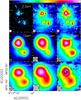 |
Fig. 1 Maps of the continuum emission towards IRAS 05137+3919 at different wavelengths (given in the top right of each panel). The labels in the top, right panel indicate the three clumps/clusters that we refer to in the text. The images have been taken from our LUCI data (2.2 μm), the IRAC database (at 3.4 and 4.6 μm), the WISE archive (12 and 22 μm), the Herschel/Hi-GAL survey (70–250 μm), and Molinari et al. (2008) (850 μm). The contours in the bottom right panel are the map of the 3.6 cm continuum emission observed by Molinari et al. (2002), while the ellipse in the bottom right denotes the corresponding angular resolution. The circle in the bottom left of each panel represents the HPBW of the corresponding image. |
2.3. IRAM 30-m telescope
The observations were performed with the IRAM 30-m antenna on Pico Veleta (Spain) on July
13 and 14, 2003. The source was mapped with HERA, a multi-beam heterodyne dual
polarization receiver, consisting of two arrays of 3×3 pixels with 24′′ spacing (Schuster et al. 2004). Areas of ~4′× 4′ and
~3′× 3′
centred around the position α(J2000) = 05h17m13 8, δ(J2000) =
39°22′20′′ were covered, respectively, in the
12CO and
C18O
J = 2 → 1
rotational transitions. The maps were made in on-the-fly mode, scanning along the right
ascension direction. The receiver was suitably rotated to allow for a sampling with
4′′ intervals in
declination, perpendicular to the scanning direction, while the data were acquired along
the scanning direction every 4′′. This results in excellent sampling of the 12′′ half-power beam width (HPBW) of the
telescope. Position switch and frequency switch were used, respectively, for the
12CO(2–1) and
C18O(2–1) line
observations. The VESPA autocorrelator was chosen as a backend, with a spectral resolution
of 0.1 km s-1 and
0.053 km s-1,
respectively, for the 12CO and C18O(2–1) lines. The pointing accuracy was regularly
checked (typically every hour) on strong, pointlike continuum sources. The data presented
in this paper are expressed in main beam brightness temperature, TMB, assuming a
forward efficiency of 0.90 and a beam efficiency of 0.52 for 12CO(2–1) and 0.55 for
C18O(2–1). The
conversion to flux density, Sν, is given by the
expression Sν(Jy) = 4.7
TMB(K). The data were reduced and
analysed by means of the GILDAS software3. The
spectra were smoothed to 0.5 km s-1 before creating channel maps of the line emission.
8, δ(J2000) =
39°22′20′′ were covered, respectively, in the
12CO and
C18O
J = 2 → 1
rotational transitions. The maps were made in on-the-fly mode, scanning along the right
ascension direction. The receiver was suitably rotated to allow for a sampling with
4′′ intervals in
declination, perpendicular to the scanning direction, while the data were acquired along
the scanning direction every 4′′. This results in excellent sampling of the 12′′ half-power beam width (HPBW) of the
telescope. Position switch and frequency switch were used, respectively, for the
12CO(2–1) and
C18O(2–1) line
observations. The VESPA autocorrelator was chosen as a backend, with a spectral resolution
of 0.1 km s-1 and
0.053 km s-1,
respectively, for the 12CO and C18O(2–1) lines. The pointing accuracy was regularly
checked (typically every hour) on strong, pointlike continuum sources. The data presented
in this paper are expressed in main beam brightness temperature, TMB, assuming a
forward efficiency of 0.90 and a beam efficiency of 0.52 for 12CO(2–1) and 0.55 for
C18O(2–1). The
conversion to flux density, Sν, is given by the
expression Sν(Jy) = 4.7
TMB(K). The data were reduced and
analysed by means of the GILDAS software3. The
spectra were smoothed to 0.5 km s-1 before creating channel maps of the line emission.
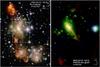 |
Fig. 2 Composite colour images obtained by combining the emission in the H2 (red), Ks (green), and H (blue) filters from the LUCI (left panel) and PISCES (right panel) data. The dashed box in the left panel indicates the region shown in the right panel. The LUCI and PISCES images cover regions, respectively, of about 0.́8 × 1.́1 and 0.́3 × 0.́4. |
 |
Fig. 3 Spectral energy distributions of clumps/clusters C1 (left panel) and C2 (right panel). The colour coding of the symbols is explained in the left panel. The triangles indicate upper limits. |
3. Results
The observational findings of our study are illustrated in the following, where we
concentrate on four main issues: the large-scale structure, extending over ~100′′, or ~4 pc, around the nominal position of
IRAS 05137+3919 – α(J2000) = 05h17m133, δ(J2000) = 39°22′14′′; the
small-scale structure, namely the region of ≲20′′, or
≲0.8 pc, imaged with the
PISCES camera; the jets and corresponding outflows (hereafter “jets/outflows”) mapped both
in the near-IR and at 3.4 mm; and the stellar clusters, spread over ~2′.
3.1. The large-scale structure
As already noted by various authors, two molecular clumps are detected in the IRAS 05137+3919 region, offset by ~30′′ along the N–S direction. In this study we focus on the northern one, but it is worth mentioning that the two clumps are likely physically close in space and not only in projection onto the plane of the sky, because their LSR velocities differ by only ~1 km s-1 (see Brand et al. 2001). Each of them hosts a stellar cluster, as pointed out by Faustini et al. (2009).
In Fig. 1 we show a number of maps of the continuum emission of IRAS 05137+3919, ranging from the near-IR to the sub-mm. We have chosen the images with the best angular resolution available in each wavelength regime. Besides confirming the previous findings, the IR images clearly indicate the existence of a third stellar cluster, located ~15′′ to the east of the southern clump and considerably fainter than the other two clusters, which are dominating the emission at all wavelengths.
For the sake of simplicity, in the following we refer to the northern clump and associated cluster (hereafter “clump/cluster”) as C1, to the southern clump/cluster as C2, and to the south-eastern cluster as C3 (see the top, right panel of Fig. 1). C1, which is the target of our investigation, is by far the most luminous at all frequencies and is the only one where free-free emission has been detected by Molinari et al. (2002), as one can see from the contour map in Fig. 1. The richness of C1 is illustrated also in the left panel of Fig. 2, where a 3-colour image of the whole region obtained from the LUCI data is shown. Here, the presence of the three clusters C1, C2, and C3 stands out clear (white colour), as well as the existence of multiple H2 jets (red colour), which we will discuss in the following.
Thanks to the Hi-GAL images, it is now possible to obtain an accurate estimate of the far-IR flux densities and hence of the luminosities of C1 and C2. We reconstructed the corresponding spectral energy distributions (SEDs) using data from the 2MASS (Skrutskie et al. 2006), Spitzer/IRAC (Werner et al. 2004; Fazio et al. 2004), IRAS, MSX (Price et al. 1999), WISE (Wright et al. 2010) archives, the Herschel/Hi-GAL survey, the SCUBA Legacy Surveys (Di Francesco et al. 2008), and the studies of Molinari et al. (2008) and Ishii et al. (1998). When possible, the flux densities were taken from the available source catalogues. In the other cases, for each clump we integrated the continuum flux inside a suitable polygon enshrouding all the emitting region, and then subtracted the background estimated through 1D cuts across the clump centre. The flux densities computed in this way, as well as the solid angles encompassed by the polygons used for the integration are given in Table A.6, while the corresponding SEDs are shown in Fig. 3. The bolometric luminosity was estimated by integrating the SED over the whole wavelength range, after linear interpolation in the Logν–LogSν plot.
For the fiducial distance of 8.3 kpc we obtain 2.4 × 10⁴L⊙ for C1 and 6.7 × 10³L⊙ for C2. These numbers agree within a factor 2 with the estimates obtained from the cluster simulations of Faustini et al. (2009) and Kumar et al. (2006), once the different distance assumed in their calculations (11.5 kpc) is taken into account.
3.2. The small-scale structure
As explained in Sect. 2, with the LBT/PISCES imaging we have attained a resolution of 80 mas or 664 au over ~20′′. This allows us to investigate in detail the innermost region of C1, which is the target of the present study. Our findings are best illustrated by the 3-colour image in the right panel of Fig. 2, where several features are worth of mention.
The “white” star to the west of the image, is very likely a foreground object, not physically related to the cluster of interest for us. The two “yellow” stars at the centre are well separated, with the one to the NE (hereafter A, after Varricatt et al. 2010) appearing slightly “redder” and hence more extincted than the other (hereafter B). While the presence of this pair was already known, in our image A splits into two sources, one, brighter, to the SW (which we call A1) and another, fainter, to the NE (A2). This is more evident in Fig. 4, where we compare the LUCI to the PISCES images. Clearly, the dramatic improvement in angular resolution obtained with AO is crucial to resolve A1 from A2, whose apparent separation is ~0.̋18 (i.e. ~1500 au).
All three sources, A1+A2+B, are likely responsible for the mid-IR emission measured by us with the San Pedro Mártir telescope, as demonstrated by Fig. 5, where we overlay the LUCI Ks image on the four images at wavelengths ranging from 8.9 to 18.7 μm. Despite the limited astrometrical accuracy (~1′′), it is clear that the bulk of the mid-IR emission arise from the same region where the near-IR emission peaks. In turn, this implies that the three sources are responsible for most of the luminosity estimated for C1 (2.4 × 10⁴L⊙), because their mid-IR emission at 12.7 and 18.7 μm corresponds to ~80% of the flux densities measured within much greater HPBWs with MSX and WISE (see Table A.6).
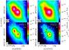 |
Fig. 4 Images of the central region of clump/cluster C1, where a pair of bright stars (A and B) had been detected in previous studies. The left and right panels refer, respectively, to Ks and H band images, while the upper and lower panels show, respectively, images obtained with the LUCI and PISCES+AO cameras. The values of the contour levels are indicated by marks in the corresponding colour scales. Note how employing AO allows us to resolve star A into the two sources A1 and A2. |
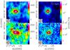 |
Fig. 5 Map of the LUCI Ks image (contours) overlaid on the mid-IR images acquired with the San Pedro Mártir 2.1 m telescope. stars (A and B) had been detected in previous studies. The wavelength of each image is indicated in the top right of the panels, while the FWHM of the PSF is drawn in the bottom left. Note that all mid-IR images have been smoothed to the resolution of the 18.7 μm image. |
An interesting feature seen in Fig. 2 is the “green” arc of continuum emission extending to the SW from B. This almost coincides with three H2 knots, which can be recognised from their red colour in the image. Whether the arc and the knots are physically related is difficult to establish, but it is possible that both are manifestations of the same phenomenon, perhaps a bow shock due to Jet 1. In any case, the knots are in all likelihood due to the interaction between the jet and the dense gas associated with C1. As explained in Sect. 1, Jet 1 was first observed by Varricat et al. (2010) and is confirmed by our images (see below).
Finally, at the top and bottom of the right panel of Fig. 2, one sees two other “red” regions of H2 line emission, shaped like bow shocks. These correspond to (part of) Jet 2, also identified by Varricat et al. (2010).
3.3. The bipolar jets/outflows
Evidence for the existence of multiple jets/outflows in the IRAS 05137+3919 region has been provided by various studies, as described in Sect. 1. Our high-resolution images shed new light on this issue, thanks to their superior sensitivity and angular resolution. Moreover, the velocity information conveyed by the 12CO maps makes it possible to discriminate between the blue- and red-shifted lobes. In Fig. 6, maps of the outflow lobes are shown, obtained by integrating the 12CO(2–1) emission over the line wings, in various velocity intervals. These maps are compared to the H2 images obtained with LUCI, which fully confirm the existence of two bipolar jets associated with C1.
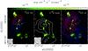 |
Fig. 6 Left: IRAM 30-m maps obtained by averaging the 12CO(2–1) over the HV line wings, overlaid on the H2 line (i.e. continuum subtracted) emission image obtained with LUCI. The integration has been performed over the LSR velocity intervals –35.65, –32.65 km s-1 (blue contours) and –17.65, –14.65 km s-1 (red contours). Contour levels range from 0.8 to 4.16 in steps of 0.48 K. The circle in the bottom left denotes the HPBW of the 30-m telescope. Right: same as left panel, for the 12CO(2–1) LV wing emission. The integration was performed over the intervals –29.65, –27.65 km s-1 (blue contours) and –22.65, –20.65 km s-1 (red contours). Contour levels range from 1.2 to 15.6 in steps of 1.44 K. Middle: map of the C18O(2–1) line emission averaged over the line, from –27.65 to –24.15 km s-1. Contour levels range from 0.54 to 1.62 in steps of 0.36 K. |
The left panel of Fig. 6 displays the high-velocity (HV) emission, which nicely coincides with Jet 2 and indicates that this jet likely lies close to the plane of the sky, because the red and blue lobes overlap significantly. The low-velocity (LV) maps shown in the right panel of the same figure look more complicate. In this case, the 12CO emission appears to be consistent with Jet 1, but significant blue-shifted emission is seen towards the red lobe, whereas no red-shifted emission is detected over the blue lobe. The complex pattern observed may be due to confusion between the LV gas and that moving at the systemic velocity (whereas such a confusion obviously cannot occur for the gas that expands at high speed in Jet 2). Also, one has to take into account that the blue-shifted emission to the SW might be partly contaminated by the bulk emission from C2 (see Sect. 3.1), whose systemic velocity differs by –1 km s-1 from that of C1. Incidentally, we note that the C1 and C2 clumps are also traced by the C18O(2–1) line map – shown in the middle panel of Fig. 6.
Despite the previous caveats, we conclude that in all likelihood the LV 12CO outflow is related to Jet 1, while the HV 12CO outflow is associated with Jet 2.
A new feature that can be seen in our image is the presence of elongated H2 line emission originating approximately from the peak of the C18O map (see Fig. 6) and extending towards W-SW over ~4′′. Clearly, this feature cannot be related to Jet 2, as the two are roughly perpendicular to each other. As for Jet 1, its SW lobe spans position angles (PA) between –179° and –145° (see the bow-shock shaped H2 knots spread over a region of 30′′), quite different from that of the new H2 feature (PA ≃−118°). We conclude that such a feature might be a third, small-scale jet previously unobserved and in the following we refer to this as Jet 3. The nature of Jet 3 will be better discussed in Sect. 4.3.
3.4. The stellar clusters
Some properties of the stellar population associated with cluster C1 can be derived from the colour-magnitude diagram of Fig. 7, where the LUCI and PISCES photometry are overlaid. The much smaller field imaged with PISCES is less contaminated by foreground field stars and allows us to characterise the colour spread of the cluster members. While the LUCI data points are distributed along a stripe close to the zero-age main sequence (ZAMS), with a number of very extincted sources (up to AV ≃ 40), the PISCES data points spread redwards of the stripe. The typical reddening of the cluster members can then be derived by reddening the ZAMS up to the nearest envelope of the PISCES data-point distribution, yielding AV = 5. Thus, the LUCI sources close to the ZAMS are essentially foreground field stars, whereas the cluster members are distributed with AV> 5 from the ZAMS (H − Ks ≳ 0.4).
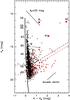 |
Fig. 7 Ks vs. H–Ks diagram of the sources retrieved in the LUCI field (black squares) and in the PISCES field (red squares). The dashed lines shows the completeness limit of the LUCI photometry (black) and the PISCES photometry (red). The black solid line is the ZAMS at a distance of 8.3 kpc (derived using the colours of Koornneef 1983 and the absolute magnitudes of Allen 1976 and Panagia 1973). The position of a few spectral types is labelled. The arrow in the top shows the effects of an extinction of AV = 20 (according to Rieke & Lebofsky 1985). The arrow in the bottom corresponds to the median disk excess vector of López-Chico & Salas (2007) for the accretion disk models of D’Alessio et al. (2005). The three brightest members of the cluster C1 are labelled, as well. |
In principle, the colour spread of the cluster members could be produced by extinction varying in the range AV≃ 5–40. However, the colour–colour diagram (J–H vs. H–Ks) of Nikoghosyan & Azatyan (2014) displays a large fraction of stellar sources with near-IR colour excess. This excess is usually caused by the presence of disks around young stars. By incorporating theoretical accreting disk models, their effect on the Ks versus H–Ks diagram has been demonstrated for disks around T Tauri stars to be accurately represented by vectors of approximately constant slope (López Chico & Salas 2007), towards brighter Ks and redder H–Ks values. More massive YSOs are usually much more embedded than T Tauri stars, and the correction proposed by López Chico & Salas (2007) is unlikely to apply to such objects. However, the presence of a spherical envelope around the disk should cause a greater decrease of H–Ks for the same variation of Ks, than in the case of a “naked” disk. Therefore, one can use the López Chico & Salas (2007) correction to obtain a lower limit to the spectral type. Assuming reddening along the arrow in the bottom of Fig. 7, after de-reddening the three objects for a minimum interstellar extinction of AV = 5, one obtains spectral types of B7 for A1 and A2, and B1 for B. Vice versa, assuming that only interstellar extinction is responsible for the reddening, along the arrow drawn in the top of Fig. 7, one estimates spectral types earlier than O8 for all three sources. The constraints set by this method on the stellar type are quite loose, but consistent with the three objects being intermediate- to high-mass stars.
Incidentally, this also proves that A1, A2, and B are part of the same system and none of them is likely to be spurious. A contaminant field star could only be a background (due to its extinction), more distant, giant or supergiant star (due to its unreddened brightness), but the probability of such a luminous object lying in the same projected area of our system is very low.
Using the extinction estimated from the colour-magnitude diagram, we can convert our Ks completeness limits into stellar mass limits. Assuming AV = 5, a cluster age of 1 Myr, a distance of 8.3 kpc, and adopting the pre-main sequence tracks of Palla & Stahler (1999), we obtain a mass completeness limit of ~0.5 M⊙ with the LUCI photometry and 0.1M⊙ with the PISCES photometry. For more extincted stars the completeness mass increases; e.g. AV = 20 yields ~2.0 M⊙ with the LUCI photometry and 0.7M⊙ with the PISCES photometry. However, we note that these values refer to “naked” stars. On the other hand, stars exhibiting a near-IR excess shine brighter at Ks, as already said, and the effective mass completeness limit decreases. The assumed age is consistent with that derived by Faustini et al. (2009), and the extinction values at the cluster peaks (derived from the sub-mm emission) listed by those authors towards C1 (AV = 18) and C2 (AV = 8) lie inside our adopted range. We also note that our Ks completeness limits are ~1 mag (LUCI) and ~2.5 mag (PISCES) less than achieved by Faustini et al. (2009), allowing us to improve on their results. A detailed analysis of the cluster stellar population will be presented in Sect. 4.1.
4. Analysis and discussion
The purpose of the following sections is to tie the large to the small scale structures in IRAS 05137+3919, and thus identify the sources powering the jets/outflows and establish their nature.
4.1. Characterization of the stellar population
A problem with young stellar clusters, especially those as distant as IRAS 05137+3919, is that their central areas are dominated by diffuse emission, source crowding, and the wings of the PSF of the brightest stars, which lead to a local worsening of the photometric completeness limit. In turn, this biases the derived properties (e.g., cluster density profile, number of members, etc.). We can assess this effect towards IRAS 05137+3919, by comparing the histograms of Ks PISCES sources and LUCI sources inside the field imaged by PISCES. These are shown in Fig. 8. We adopted a bin width of 0.5 mag, larger than the maximum uncertainty on the PISCES photometry. Clearly, the LUCI histogram peak is brighter than the LUCI completeness limit estimated all over the LUCI field of view. In addition, the number of Ks sources brighter than the completeness limit and retrieved with LUCI is less than those detected with PISCES. An interesting characteristic of the PISCES histogram is its double peak. While the fainter peak is due to increasing incompleteness in sampling the stellar background population, the brighter peak is very likely an intrinsic feature of the C1 cluster population, as it lies well above the completeness limit of PISCES (red dotted line in Fig. 8).
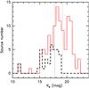 |
Fig. 8 Histograms of the distribution of Ks source magnitudes inside the field of view of PISCES. The red solid line indicates PISCES sources, the black dashed one LUCI sources. The vertical black and red dotted lines show, respectively, the completeness limit of the LUCI and PISCES Ks photometries, estimated from the whole corresponding field (see text). |
How much the degraded completeness limit in the innermost, densest part of C1 affects the observed cluster properties can be assessed by plotting the surface radial density of Ks sources as derived in concentric annuli centered at the brightest cluster member (i.e. B). As shown in Fig. 9, when the LUCI sources are replaced by the PISCES ones inside the field of view of PISCES (and only counting sources with Ks≤ 17.75, the LUCI completeness limit), the surface density doubles at the centre. The outermost annuli give an approximate measure of the field star density, which may be subtracted from the central peak to derive the real stellar density of cluster C1. Note that the density plateau between 1 pc and 2 pc is due to the small clusters C2 and C3, rather than to a halo of members around C1.
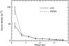 |
Fig. 9 Surface radial density of Ks sources derived in concentric annuli centred at the position of B, the brightest cluster member. The solid line indicates the density as computed from the LUCI photometry. The dashed line indicates the density computed by replacing the LUCI photometry with the PISCES photometry inside the area corresponding to the field of view of PISCES. The sources are counted up to the LUCI completeness limit (i.e. Ks ≃ 17.75). The errorbars show the Poissonian count fluctuations. |
The number of cluster members can be derived from the radial surface density distribution in Fig. 9 like the “richness indicator” Ic (see e.g. Testi et al. 1998). This implies integrating on the inner annuli and using the outermost annuli to estimate the background correction. We have integrated up to a radius of 0.97 pc and 1.93 pc to obtain, respectively, the total richness indicators for C1 (Ic = 87 ± 2 stars) and C1+C2+C3 (Ic = 120 ± 4 stars). For this purpose, we used the radial surface density corrected with the PISCES photometry (dashed line in figure). We note that Ic is much larger than obtained by Faustini et al. (2009), due both to our crowdness correction and more sensitive completeness limit. Our estimate of 87 stars pc-2 seems comparable to the values derived by Testi et al. (1999) for their sample of Herbig Be stars. However, one must take into account that their sensitivity is better than ours by a couple of magnitudes at Ks, after suitable scaling for the smaller distance of their targets (less than ~1 kpc). Therefore, we may reasonably conclude that C1 is significantly richer than the clusters around Herbig Be stars. Once more, we speculate that this might be related to the age of the cluster, as ours is younger than those of Testi et al., being associated with molecular gas and powerful outflow activity.
Finally, Ic can be converted into a total number of cluster members provided a suitable initial mass function (IMF) is assumed. However, such a conversion is hindered by the uncertainty on the mass completeness limit. The latter depends on the real distribution of the extinction, which we cannot derive from our data, and stellar age. We have quoted a mass completeness limit (corresponding to Ks = 17.75) between 0.5 and 2 M⊙, but this should be further decreased if the cluster is younger than the adopted value of 1 Myr. In addition, in clusters that young, a high fraction of low-mass stars are still associated with a circumstellar disk and do exhibit a near-IR excess (see Sect. 3.4), which makes their detection easier. If we roughly assume that the Ic value is representative of >1 M⊙ stars, by considering a standard IMF (e.g. Scalo 1998), then the total number of C1+C2+C3 members (down to 0.1 M⊙) would be ~700. In this case, the IMF would predict 2 members with M ≳ 15M⊙. We conclude that our cluster analysis supports the existence of 2–3 early B-type stars, consistent with our estimates of the luminosities of sources A1, A2, and B.
4.2. Characterization of the jets/outflows
As illustrated in Sect. 3.3, evidence for the existence of up to 3 H2 jets is seen in the IRAS 05137+3919 region. Here we focus our analysis on the most prominent of these, namely Jet 1 and Jet 2, and postpone the discussion of Jet 3 to Sect. 4.3.1.
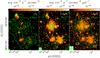 |
Fig. 10 Left: overlay of the 4.5 μm Spitzer/IRAC image (contours) on the LBT/LUCI image of the H2 line emission (continuum subtracted). Contours are drawn in 5 logarithmic steps from 1 to 60 MJy/sterad. The angular resolution of the contour maps is indicated by the circle in the bottom left. Middle: same as left panel, for the overlay of the HCO+(1–0) line OVRO map by Molinari et al. (2002), corrected for primary beam attenuation, on our LBT/LUCI Ks-filter image. The HCO+ map has been obtained by averaging the emission between –28.76 and –20.78 km s-1. Contour levels range from 57 to 342 in steps of 95 mJy/beam. The dashed circle denotes the primary beam of the OVRO interferometer. Right: same as left panel, for the overlay of the WISE 3.4 μm map on the LBT/LUCI H-filter image. Contours are drawn in 6 logarithmic steps from 1 to 76 MJy/sterad. Labels C1, C2, and C3 have the same meaning as in Fig 1. |
4.2.1. Jet 1
While the existence of Jet 2 is out of question, due to its nice bipolar and well collimated morphology, the structure of Jet 1 is more complex and casts some doubts on the unicity of this jet. A priori, one might consider the possibility that the complex pattern of this jet might be due to precession. Although such a hypothesis cannot be ruled out, we prefer not to discuss it any further, because a precessing jet should describe an S-shaped pattern on the plane of the sky (see e.g. Fig. 18 of Cesaroni et al. 2005), while no convincing evidence of such a pattern is seen in our case. We thus attempt to explain the observed features with the simplest possible model, without invoking additional mechanisms besides expansion.
Is it possible that Jet 1 is in fact the result of the combination of multiple, distinct jets? To investigate this issue and establish the origin of the jets, in Fig. 10 we compare our near-IR images with other IR and molecular line maps. In the left panel we show an overlay of the 4.5 μm Spitzer/IRAC map on the LUCI image of the H2 line emission. One sees that basically all of the H2 knots belonging to Jet 1 coincide with peaks of the 4.5 μm emission. This is consistent with the presence of unresolved H2 lines in the bandwidth covered by the Spitzer/IRAC 4.5 μm filter. The middle and right panels clearly illustrate the presence of three stellar clusters, already discussed in Sect. 3.1, traced by the low-resolution 3.4 μm WISE image and resolved in our 1.6 and 2.2 μm LUCI images. We also compare the near-IR emission to the HCO+(1–0) interferometric map of Molinari et al. (2002), to show that the brightest cluster is associated with a dense molecular core in C1, and lies close to the geometrical centre of jets 1 and 2. We thus believe it is very reasonable to assume that the YSOs powering these jets/outflows lie inside C1, and we will base all our reasoning on such an assumption.
The left panel of Fig. 10 shows that the SW lobe of Jet 1 consists of a number of bow-shock-like features spread over a broad region, unlike the NE lobe, which appears well collimated. One may hence wonder whether Jet 1 is not a single jet, but the result of multiple jets overlapping in the plane of the sky. A priori, the H2 knots falling in the regions corresponding to clusters C2 and C3 might belong to small jets powered by stars of those two clusters. However, careful inspection of the H2 image reveals that all of the knots to the SW have bow-shock shapes pointing to the S-SW, which is inconsistent with the driving source to be located in C2 or C3. We thus believe that in all likelihood these knots belong to Jet 1, whose origin lies in cluster C1. If this is the case, why does the SW lobe appear so much less collimated than the NE lobe? A possibility is that the two lobes are intrinsically similar, but the SW one looks wider because it is impinging against C2 and C3, where one sees H2 shocked emission. The NE lobe, in contrast, is expanding through lower density medium, which could confine the H2 emission to internal shocks along the jet axis (see e.g. Stone et al. 1997).
4.2.2. Jet 2
Jet 2 looks much better defined than Jet 1 and is clearly centred on the peak of the molecular clump C1, as shown by the comparison with the HCO+ line emission (middle panel of Fig. 10). As already noted, the 12CO(2–1) outflow appears to mirror the pattern of the H2 jet, thus allowing a kinematical analysis of the jet/outflow structure. For this purpose, we assume that the YSO powering this outflow coincides with one among A1, A2, and B. Evidence in favour of this hypothesis will be provided in Sect. 4.3. In Fig. 11 we show the position–velocity (PV) plot along the Jet 2 axis, namely for PA = −17°. While the LV emission (between −30 km s-1 and −22 km s-1) is confused by the extended 12CO bulk emission close to the systemic velocity of ~−25 km s-1 (Brand et al. 2001), beyond this interval one sees both red- and blue-shifted emission, both at positive (~10′′) and negative (~–10′′) offsets. However, the mean velocity of the emission is slightly skewed to the red at positive offsets and to the blue at negative ones. We will demonstrate that such a difference can be explained by a (small) inclination of the outflow with respect to the plane of the sky.
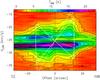 |
Fig. 11 Position–velocity plot of the 12CO(2–1) line emission along the direction matching the axis of Jet 2, i.e. with PA = −17°. The values of the contour levels are shown in the colour scale at the top of the figure. The offset is measured from an arbitrary position. The vertical and horizontal dashed lines indicate, respectively, the position of stars A+B and the systemic velocity of the associated clump. The white solid pattern encloses the region inside which emission is expected for the conical jet model that best fits the data (see text). The dashed pattern corresponds to the same model with a slightly different inclination angle (10° instead of 2°; see text). |
To prove our hypothesis and obtain an estimate of the inclination angle (important for
a correct estimate of the outflow parameters), we have applied the conical outflow model
of Cesaroni et al. (1999) to our case. This is a
simple-minded model that assumes that the outflowing material is confined inside a cone
with aperture angle θ, inclination angle φ with respect to the
plane of the sky, length of each lobe R0, and expansion velocity
V =
V0
(R/R0). The model
computes the pattern inside which emission is expected in the PV plot. Reasonable
guesses for the input parameters θ, φ, and V0 can be obtained by solving Eqs.
(A.6)–(A.8) of Cesaroni et al. (1999). For this
purpose, we need an estimate of the projection of θ on the plane of the
sky, θ′,
and the maximum and minimum velocities along the line of sight (relative to the systemic
velocity of –25 km s-1) observed in each lobe,
 and
and
 (in the notation of Cesaroni et al.
1999). The latter are obtained from Fig. 11 and are, respectively, 8.8 km s-1 and 7 km s-1, while θ′ can be estimated from
the jet/outflow maps in Fig. 6 and is about
15°–30°. The solution of the three equations is
φ ≃ 0°,
θ′ ≃ θ ≃
15°–30°,
and V0≃ 16–31 km s-1. Since the outflow axis lies
very close to the plane of the sky, R0 can be obtained directly from the
outflow maps and is ~14′′.
(in the notation of Cesaroni et al.
1999). The latter are obtained from Fig. 11 and are, respectively, 8.8 km s-1 and 7 km s-1, while θ′ can be estimated from
the jet/outflow maps in Fig. 6 and is about
15°–30°. The solution of the three equations is
φ ≃ 0°,
θ′ ≃ θ ≃
15°–30°,
and V0≃ 16–31 km s-1. Since the outflow axis lies
very close to the plane of the sky, R0 can be obtained directly from the
outflow maps and is ~14′′.
The best fit was obtained by slightly varying the input values around these guesses. and is represented by the solid pattern in Fig. 11 (computed from Eqs. (A.2) and (A.3) of Cesaroni et al. 1999), which corresponds to R0 = 14″, V0 = 30 km s-1, θ = 15°, and φ = 2°. The model mimics the shape of the 12CO emission quite well and proves that the outflow axis is indeed almost perpendicular to the line of sight. It is instructive to check how much the pattern would change for a slightly different inclination angle, e.g. φ = 10°. This is shown by the white, dashed lines in Fig. 11, which are significantly offset from the best fit. We thus conclude that the uncertainty on the inclination is very small.
It is also useful to derive the main outflow parameters. These have been computed by integrating the 12CO(2–1) line emission over the lobes, in the velocity intervals −35.15, −29.65 km s-1 and −21.15, −16.65 km s-1. In the calculation we assume LTE at a temperature of 30 K, optically thin emission, and a 12CO abundance relative to H2 of 10-4. The resulting parameters have been divided by the outflow dynamical time scale tdyn = R0/V0 ≃ 0.56 pc/30 km s-1 ≃ 1.8 × 10⁴ yr, to obtain the mass loss rate, Ṁ = 4.2 × 10⁻⁴M⊙ yr-1, and momentum rate Ṗ ≃ 9.2 × 10⁻³M⊙ km s-1 yr-1. The latter has been corrected for the inclination of the flow with respect to the line of sight, assuming the outflow model described above. From Ṗ one can estimate the bolometric luminosity (L) of the source powering the outflow by means of the relationship between Log(Ṗ) and Log L derived by Wu et al. (2004). From their Fig. 7 one obtains L ≃ 3 × 10⁴L⊙, but with a large uncertainty which allows for values ranging from 103L⊙ to almost 106L⊙. While this result does not permit us to set tight constraints on the nature of the YSO powering Jet 2, it is consistent with the bolometric luminosity estimate (2.4 × 10⁴L⊙) obtained from the SED (see Sect. 3.1) and confirms that one is indeed dealing with a high-mass star.
4.3. Identification of the sources driving the jets
Until now, we have assumed that the YSOs powering the jets/outflows in IRAS 05137+3919 are located close to the centre of the cluster shown in Fig. 2. Here, we want to prove that the origin of the jets/outflows is to be searched among the three brightest sources: A1, A2, and B. For this purpose, in Fig. 12 we present three images of the H2 jets, which progressively zoom into the neighbourhood of the three objects. For the sake of comparison, we also draw the borders of the conical jet model described in Sect. 4.2.2 (short-dash blue lines), centred on the position of B. This looks like an obvious choice, because star B lies right along the symmetry axis of Jet 2, unlike A1 and A2. Moreover, if the origin of the flow were shifted along that axis, the model in Fig. 11 could not reproduce the blue-red symmetry of the observed PV plot. Although one cannot rule out the possibility that another deeply embedded, yet undetected star within a couple of arcsec from B is powering Jet 2, this appears quite unlikely for the following reason. A1, A2, and B lie at the very peak of the molecular line and mm continuum emission, where the column density should be highest (see Fig. 13). Despite this fact, all of them have been detected in our images, even at H-band, which makes it difficult to believe that any other similar (or more luminous) star in the neighbourhood, where the column density is lower, could be so embedded to be undetectable. We thus conclude that star B is likely to be powering Jet 2.
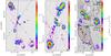 |
Fig. 12 Left: LUCI image of the H2 line emission (continuum subtracted) tracing the jets in IRAS 05137+3919. The artefact due to continuum subtraction at the position of stars A1, A2, and B has been blanked (white area). The contours are a map of the continuum emission measured in the Ks filter. The contour levels have been chosen to show only the brightest stars in the field. The red long-dash and blue short-dash lines indicate, respectively, the borders of Jet 1 and Jet 2. Middle: same as left panel, for a smaller region centred on the jets’ origin. Right: same as left panel, for a comparison between the H2 line and Ks continuum images taken with LUCI (top) and PISCES (bottom). The red points and corresponding arrows denote the H2O maser spots and associated relative proper motions measured by Honma et al. (2011). |
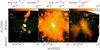 |
Fig. 13 Left: overlay of the contour map of the HCO+(1–0) line (from Molinari et al. 2002) obtained by averaging the emission between –27.08 and –23.72 km s-1, on the H2 line (i.e. continuum subtracted) LUCI image. Contour levels range from 150 to 420 in steps of 90 mJy/beam. Like in Fig. 12, the area around stars A1, A2, and B has been blanked to mask an artefact caused by the continuum-subtraction process. Middle: overlay of the contour map of the 3.4 mm continuum emission (from Molinari et al. 2002) on the 2.2 μm continuum LUCI image. Contour levels range from 2.64 to 4.4 in steps of 0.88 mJy/beam. Right: overlay of the contour map of the 3.6 cm continuum emission (from Molinari et al. 2002) on the 2.2 μm continuum PISCES image. Contour levels range from 0.069 to 0.161 in steps of 0.023 mJy/beam. |
In Fig. 12, we also draw a tentative pattern for Jet 1 (red long-dash lines), under the working hypothesis that this originates from A1 or A2. The aperture angle of the jet is greater than for Jet 1 (~20°), consistent with the 12CO outflow map in Fig. 6. In Fig. 13 one sees that the peak of the 3.6 cm continuum emission (Molinari et al. 2002) is roughly consistent with the position of A1/A2, with a tail of emission extending to the NE, in the direction of Jet 1. This alignment suggests that at least part of the free-free emission could originate from a thermal jet tracing the root of Jet 1. The most direct evidence for a tight association between A1/A2 and Jet 1 is presented in the right panel of Fig. 12, where we plot the relative proper motions of the H2O masers observed by Honma et al. (2011). These are clearly expanding along the Jet 1 axis, from a centre whose position is compatible (within the astrometrical uncertainty of the IR images) with that of the A1/A2 pair. Since water masers are believed to form in shocks, the observed association indicates that the maser motions are tracing the innermost part of the jet.
This result casts some doubt on the interpretation of A1 and A2 as a binary system. Since the two objects are aligned along the Jet 1 axis, one should consider the possibility that they are the lobes of a small bipolar reflection nebula. Such an interpretation is supported by a comparison in the PISCES Ks image between the shapes of A1 and A2, on the one hand, and B, on the other hand. While the latter appears approximately circular, A1 and A2 are slightly elongated, respectively, in the E–W and N–S directions. Since the separations of the sources from the guide star are similar, the different shapes are unlikely to be due to anisoplanatism. We used DAOPHOT in IRAF to compare the PSFs by performing some experiments on the Ks image. We found that when using B as the reference PSF, after PSF subtraction through a fit, both A1 and A2 are oversubtracted, consistent with them being slightly more extended. Moreover, when using A2 as the reference PSF, after subtraction A1 is still oversubtracted, whereas B is now undersubtracted, consistent with A1 being slightly more extended than A2. In summary, the PSFs of A1 and A2 differ from each other and that of A1 departs the most from a stellar PSF.
In the light of the previous results, it seems plausible that A1 and A2 are not point-like stars but the marginally resolved lobes of a bipolar reflection nebula. In this case, the dark lane between the lobes could be due to a circumstellar disk, with size on the order of the separation between A1 and A2, namely ~1500 au. This value is similar to the diameter of disks around high-mass (proto)stars (see Cesaroni et al. 2007). Note that the distance between the two maser spots is ~1120 au, slightly less than the separation A1–A2, in agreement with a scenario where the masers trace the expansion of the jet in the densest part of it, closer to the star than the IR lobes, as observed in other similar objects (e.g. the massive protostar IRAS 20126+4104; see Cesaroni et al. 2013). We note also that the brightest source, A2, lies to the SW, namely in the direction of the blue-shifted lobe of jet1, consistent with the expectation that the brighter lobe of a reflection nebula is the one pointing to the observer.
In conclusion, one should seriously consider the possibility that the pair A1/A2 is not a binary system, but a bipolar nebula associated with a disk+jet system from a massive star.
4.3.1. Jet 3
Finally, we investigate the nature of (putative) Jet 3. The right panel of Fig. 12 shows an enlargement of it, with a comparison between the LUCI and PISCES images. At lower angular resolution the H2 emission seems to trace an elongated lobe, made out of 3 knots, with the northernmost of these lying ~1′′ to the south of A1/A2. This structure suggests that one might indeed be observing a jet originating from another (lower-mass) star beside A1, A2, and B. However, in the high resolution image the first knot to the E disappears, whereas the others are still visible albeit partly resolved out. In our opinion, this indicates that the northern knot is an artefact due to residuals in the subtraction of the Ks continuum from the H2 filter, in the LUCI images. If this is the case, the other knots could be associated with Jet 1. In conclusion, while the presence of a third jet from another (possibly low-mass) YSO in the cluster cannot be excluded, we prefer to consider the simplest possible scenario, where all H2 knots are explained with only two jets (Jet 1 and Jet 2). Only future, more sensitive images of the jet/outflow structure could help us to establish the correct interpretation.
4.4. Nature of A1/A2 and B
The luminosity measured in Sect. 3.1 sets an upper limit of ~2.4 × 10⁴L⊙ to that of the most massive member of cluster C1. There is little doubt that the luminosity must be dominated by A1/A2 and B, as these are by far the brightest sources in the field, with A2 being the brightest at Ks-band (11.2 mag) and the one with the largest colour index (H–Ks = 3.8 mag). We deduce that the corresponding star is the most massive in the cluster, no matter whether A2 is a real star or the lobe of a reflection nebula. Actually, in the latter case, one would see only part of the photons emitted by the embedded star, thus lending further support to our previous statement that this is the most massive member of cluster C1.
When discussing the luminosity of C1, is worth taking into account the inclination of the jets with respect to the line of sight. We have seen that Jet 2 lies close to the plane of the sky. A similar conclusion is likely to hold also for Jet 1, if A1 and A2 are reflection nebulae, because if the jet axis were close to the line of sight the nebulosity associated with the red-shifted lobe would not be detected. It has been shown (see Fig. 10 of Whitney et al. 2003) that beaming of photons along the jet axis, the so-called “flashlight effect”, may lead to an underestimate of the source luminosity by a factor 2 – or even more (see Zhang et al. 2013). We thus caution that the luminosity of C1 might be significantly greater than our previous estimate of ~2.4 × 10⁴L⊙.
We have attempted a more precise estimate of the total luminosity of A1+A2+B by fitting only the 2MASS J, H, Ks, our 8.9–18.7 μm, and the L-band measurements by Ishii et al. (1998), with the on-line model fitter4 by Robitaille et al. (2013). The other fluxes in Fig. 3 were set as upper limits. In the calculations we have fixed the distance to 8.3 kpc and assumed an interstellar visual extinction AV< 5 (see Rowles & Frobrich 2013). Despite the loose constraints, the first 50 best-fit models span a relatively small range in luminosity, Lmod = (4.4–15) × 103L⊙. Taken at face value, this implies that 38–82% of the luminosity of cluster C1 is due to the lower-mass members of it. A range of values for the maximum stellar mass among A1, A2, and B is obtained under the two opposite assumptions that either only one star is responsible for Lmod, or all three stars equally contribute to Lmod. Correspondingly, one obtains a range for the most massive star in the cluster of 8–15 M⊙ (see e.g. Diaz-Miller et al. 1998).
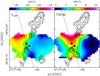 |
Fig. 14 Left: overlay of the H2 line (i.e. continuum subtracted) LUCI image (contours) on a map of the peak LSR velocity of the HCO+(1–0) line observed by Molinari et al. (2002). The artefacts due to continuum subtraction in the H2 image have been blanked as already done in Fig. 12. The dashed lines represent the axes of Jet 1 and Jet 2, while the two black points indicate the positions of stars A1+A2 and B. Right: same as left panel, for the HCO+(1–0) line full width at half maximum. |
Alternatively, the luminosity of the most massive star(s) can be derived from the radio continuum flux density, assuming that this originates from an optically thin Hii region around an early-type star. One can compute the stellar Lyman continuum emission, and hence the luminosity, as done by Molinari et al. (2002), who obtain a Lyman continuum photon rate of ~2 × 1045 s-1 (after scaling from their distance of 11.5 kpc to ours of 8.3 kpc), corresponding to a luminosity of ~6 × 10³L⊙ and a stellar mass of ~11 M⊙. These numbers appear to agree quite well with our previous estimates; however one should keep in mind that the radio continuum emission could be due to a thermal jet rather than a photoionised Hii region. Multi-wavelength radio maps with better angular resolution are needed to establish the nature of this emission.
Finally, we attempt an estimate of the luminosity using the H2 line emission. Following Caratti o Garatti et al. (2006), one may relate L to the luminosity in the H2 line, LH2, by means of the expression Log [ LH2(L⊙) ] = (0.58 ± 0.06) Log [ L(L⊙) ] − (1.4 ± 0.06) which holds for jets associated with stars from 0.1 to 105L⊙ (see Caratti o Garatti et al. 2013). We have computed LH2 following the recipe of Caratti o Garatti et al. (2006), namely integrating the emission over all H2 knots belonging to the jet and then multiplying by 10 to correct for the energy radiated in the other non-observed H2 transitions. A further correction for the interstellar extinction must be applied. The Robitaille model fit previously described corresponds to a range AV = 1.2–2.9, which translates into a correction factor at the wavelength of the H2 filter (2.12 μm) of 10A2.12 μm/ 2.5 = 1.13–1.35 (where we assume a ratio A2.12 μm/AV = 0.112; see Rieke & Lebofsky 1985). From the LUCI H2 image we obtain LH2 ≃ 7.4 L⊙ for Jet 1 and LH2 ≃ 1.5 L⊙ for Jet 2, which imply, respectively, L ≃ 8 × 10³L⊙ and L ≃ 5 × 10²L⊙. These values are in good agreement with the those previously obtained from the IR fluxes and free-free radio emission, and confirm that star B could be powering Jet 2, while Jet 1 could originate from A1+A2, the most massive star(s) in cluster C1.
4.5. Structure and kinematics of the molecular core
The interferometric observations of Molinari et al. (2002) have established the presence of a compact molecular core, where stars A1+A2 and B seem to be embedded. It is interesting to investigate the structure and kinematics of this core in relationship to the observed jets and stars. In Fig. 13 we plot a map of the HCO+(1–0) bulk emission (contours in the left panel) on the image of the H2 line emission. Note that the HCO+ map in this figure differs from that in the middle panel of Fig. 10 because the latter has been obtained by integrating the HCO+ emission over the whole line profile, whereas the former considers only a small range around the systemic velocity. The shape of the core appears elongated E–W, namely roughly perpendicular to Jet 1 and Jet 2.
In Fig. 14 we analyse the velocity field of the core, through maps of the peak velocity and line full width at half maximum (FWHM). These parameters have been obtained with a Gaussian fit to the HCO+ line profile, pixel by pixel, over the whole region where HCO+ emission was detected above 5σ. A clear velocity gradient is present in the E–W direction, with A1, A2 and B lying at positions where the velocity equals the systemic velocity of –25 km s-1. The line FWHM is minimum to the E and W of the core, and attains its maximum to the N and S, approximately where the jets emerge from the core. This suggests that the core is significantly perturbed by the material expanding along those directions. The question is how to interpret the shift observed in the peak velocity. It is possible that such a shift is due to Jet 1, whose red–blue symmetry looks consistent with the direction joining the maximum (located to the NE) and minimum (to the SW) HCO+ peak velocities. However, maximum/minimum velocities are seen also to the SE/NW and looking at the whole velocity field one gets the impression that the mean velocity gradient is directed E–W rather than NE–SW.
With this in mind, one is tempted to interpret the velocity gradient as rotation of the core about the jets’ axes. Under this hypothesis, the mass needed to guarantee rotational equilibrium of an oblate core with angular diameter ~8′′ and rotation velocity ~2 km s-1 is ~150 M⊙. This may be compared with the mass of the core computed from the 3.4 mm continuum flux of 21 mJy (see Table 3 of Molinari et al. 2002). In our calculation we adopt a dust absorption coefficient of 0.01 cm2 g-1 at 1.3 mm (for a gas-to-dust mass ratio of 100 and using the estimates of Ossenkopf & Henning 1994), scaling like ∝ λ− β with β = 1, and a dust temperature of 60 K (estimated from the ratio of the NH3(1,1) and (2,2) inversion transitions observed in the RMS survey5 (Lumsden et al. 2013). Under these assumptions we obtain ~120 M⊙, with a large error due to the uncertainty on the dust absorption coefficient and dust temperature. Nonetheless, the core mass is of the same order of magnitude as the dynamical mass, consistent with the hypothesis of a core in rotational equilibrium.
Based on the above, one may speculate that the stellar cluster is the result of the fragmentation of a rotating core, yielding a couple of massive stars with (remnants of) circumstellar disks, whose observable manifestations are Jet 1 and Jet 2. Further interferometric observations of the dense molecular gas are required to lend support to the proposed scenario.
5. Summary and conclusions
We performed observations at near-IR, mid-IR, and millimetre wavelengths of the star forming region IRAS 05137+3919 to investigate the complex jet structure and the associated stellar cluster(s). The dramatically improved sensitivity and resolution as well as the broad frequency coverage obtained by complementing our data with archival data, allow us to obtain a number of results:
-
We identify 3 stellar clusters (C1, C2 and C3) in the region, with the two richest ones being embedded in molecular clumps.
-
The luminosity of the richest cluster, C1, which contains the brightest stars, is ~2.4 × 10⁴L⊙, a value typical of early B-type stars. We indeed conclude that the most massive star in C1 has a mass of ~8–15 M⊙.
-
Employing adaptive optics, we resolve the densest part of cluster C1 thus significantly increasing the number of known cluster members with respect to previous estimates based on lower resolution images. In particular, we find that of the two brightest stars, A and B, previously identified, the first is actually made of two distinct sources that we name A1 and A2.
-
The stellar cluster C1 turns out to be richer and less concentrated than those observed by other authors around Herbig Be stars and we thus speculate that the difference could be due to an evolutionary effect.
-
We confirm the existence of (at least) 2 bipolar jets/outflows and demonstrate that they originate from C1. Using various approaches, we come to the conclusion that both jets must be powered by early B-type stars.
-
By comparing the geometry and velocity field of the jets/outflows to the properties and location of the stars, we propose that the smaller jet is powered by the more luminous and less embedded star B, whereas the largest jet originates from the pair A1+A2.
-
We speculate that A1+A2 could be a small bipolar nebula along the jet axis, outlining a disk of ~103 au seen in silhouette. This hypothesis is supported by the fact that the molecular gas appears to rotate (although on a much larger scale of ~0.2 pc) about the jet axis.
Our findings demonstrate the potential of sub-arcsecond resolution in the near IR to investigate high-mass star forming regions and call for further imaging at (sub)millimetre wavelengths with comparable resolution to shed light on the circumstellar environment and its connection with the large-scale jets. To date, only the ALMA interferometer can resolve structures as small as ~100 mas and thus allow one to study the gas kinematics and physical properties on scales ≲100 au in IRAS 05137+3919 and similar regions.
Online material
Appendix A: Appendix A:
Coordinates, magnitudes, and colour of the sources identified in the LUCI field. The symbol “–” indicates a non-detection.
Coordinates and fluxes of the H2 knots belonging to Jet 1.
Coordinates and fluxes of the H2 knots belonging to Jet 2.
Coordinates and fluxes of the H2 knots belonging to Jet 3.
Coordinates, magnitudes, and colour of the sources identified in the PISCES field. The symbol “–” indicates a non-detection.
Continuum flux densities, Sν, of clumps C1 and C2 and corresponding solid angles, Ω, over which the integration was performed.
IRAF is distributed by the National Optical Astronomy Observatory, which is operated by the Associated Universities for Research in Astronomy, Inc., under cooperative agreement with the National Science Foundation.
The GILDAS software has been developed at IRAM and Observatoire de Grenoble – see http://www.iram.fr/IRAMFR/GILDAS
Acknowledgments
It is a pleasure to thank Francesca Bacciotti and Daniele Galli for instructive discussions on jets from YSOs. M.T. acknowledges support from UNAM/PAPIIT grant No. IN-101813. This work is based in part on observations made with the Spitzer Space Telescope, which is operated by the Jet Propulsion Laboratory, California Institute of Technology under a contract with NASA. This publication also makes use of data products from the Two Micron All Sky Survey, which is a joint project of the University of Massachusetts and the Infrared Processing and Analysis Center/California Institute of Technology, funded by the National Aeronautics and Space Administration and the National Science Foundation.
References
- Allen, C. W. 1976, Astrophysical Quantities, 3rd edn. (London: Athlone press) [Google Scholar]
- Brand, J., Cesaroni, R., Palla, F., & Molinari, S. 2001, A&A, 370, 230 [NASA ADS] [CrossRef] [EDP Sciences] [Google Scholar]
- Caratti oGaratti, A., Giannini, T., Nisini, B., & Lorenzetti, D. 2006, A&A, 449, 1077 [NASA ADS] [CrossRef] [EDP Sciences] [Google Scholar]
- Caratti o Garatti, A., Stecklum, B., Linz, H., Garcia Lopez, R., & Sanna, A. 2013, Protostars and Planets VI, Heidelberg, July 15–20, Poster #1K043 http://www.mpia-hd.mpg.de/homes/ppvi/posters/1K043.pdf [Google Scholar]
- Cesaroni, R., Felli, M., Jenness, T., et al. 1999, A&A, 345, 949 [NASA ADS] [Google Scholar]
- Cesaroni, R., Neri, R., Olmi, L., et al. 2005, A&A, 434, 1039 [NASA ADS] [CrossRef] [EDP Sciences] [Google Scholar]
- Cesaroni, R., Galli, D., Lodato, G., Walmsley, C. M., & Zhang, Q. 2007, in Protostars and Planets V, eds. B. Reipurth, D. Jewitt, & K. Keil (Tucson: Univ. of Arizona Press), 197 [Google Scholar]
- Cesaroni, R., Massi, F., Arcidiacono, C., et al. 2013, A&A, 549, A146 [NASA ADS] [CrossRef] [EDP Sciences] [Google Scholar]
- D’Alessio, P., Merín, B., Calvet, N., Hartmann, L., & Montesinos, B. 2005, Rev. Mex. Astron. Astrofis., 41, 61 [NASA ADS] [Google Scholar]
- Diaz-Miller, R. I., Franco, J., & Shore, S. N. 1998, ApJ, 501, 192 [NASA ADS] [CrossRef] [Google Scholar]
- Di Francesco, J., Johnstone, D., Kirk, H., MacKenzie, T., & Ledwosinka, E. 2008, ApJS, 175, 277 [NASA ADS] [CrossRef] [Google Scholar]
- Esposito, S., Riccardi, A., Quirós-Pacheco, F., et al. 2010, Appl. Opt., 49, 174 [Google Scholar]
- Esposito, S., Riccardi, A., Pinna, E., et al. 2011, in Astronomical Adaptive Optics Systems and Applications IV, eds. R. K. Tyson, & M. Hart, Proc. SPIE, 8149, 814902 [Google Scholar]
- Esslinger, O, & Edmunds, M. G., 1998, A&AS, 129, 617 [NASA ADS] [CrossRef] [EDP Sciences] [Google Scholar]
- Faustini, F., Molinari, S., Testi, L., & Brand, J. 2009, A&A, 503, 801 [NASA ADS] [CrossRef] [EDP Sciences] [Google Scholar]
- Fazio, G. G., Hora, J. L., Allen, L. E., et al. 2004, ApJS, 154, 10 [NASA ADS] [CrossRef] [Google Scholar]
- Honma, M., Hirota, T., Kan-Ya, Y., et al. 2011, PASJ, 63, 17 [NASA ADS] [Google Scholar]
- Ishii, M., Nagata, T., Sato, S., Watanabe, M., & Yao, Y. 1998, ApJ, 116, 868 [Google Scholar]
- Ishii, M., Nagata, T., Sato, S., et al. 2001, ApJ, 121, 3191 [Google Scholar]
- Ishii, M., Hirao, T., Nagashima, C., Nagata, T., & Sato, S. 2002, ApJ, 124, 430 [Google Scholar]
- Koornneef, J. 1983, A&A, 128, 84 [NASA ADS] [Google Scholar]
- Kumar, M. S. N., Keto, E., & Clerkin, E. 2006, A&A, 449, 1033 [NASA ADS] [CrossRef] [EDP Sciences] [Google Scholar]
- López-Chico, T. A., & Salas, L., 2007, Rev. Mex. Astron. Astrofis., 43, 155 [NASA ADS] [Google Scholar]
- Lumsden, S. L., Hoare, M. G., Urquhart, J. S., et al. 2013, ApJS, 208, 11 [NASA ADS] [CrossRef] [Google Scholar]
- McCarthy, D. W., Jr., Ge, J., Hinz, J. L., Finn, R. A., & de Jong, R. S. 2001, PASP, 113, 353 [NASA ADS] [CrossRef] [Google Scholar]
- Molinari, S., Brand, J., Cesaroni, R., & Palla, F. 1996, A&A, 308, 573 [NASA ADS] [Google Scholar]
- Molinari, S., Brand, J., Cesaroni, R., Palla, F., & Palumbo, G. G. C. 1998, ApJ, 336, 339 [Google Scholar]
- Molinari, S., Testi, L., Rodríguez, L. F., & Zhang, Q. 2002, ApJ, 570, 758 [NASA ADS] [CrossRef] [Google Scholar]
- Molinari, S., Pezzuto, S., Cesaroni, R., et al. 2008, A&A, 481, 345 [NASA ADS] [CrossRef] [EDP Sciences] [Google Scholar]
- Molinari, S., Swinyard, B., Bally, J., et al. 2010, PASP, 122, 314 [NASA ADS] [CrossRef] [Google Scholar]
- Nikoghosyan, E. H., & Azatyan, N. 2014, Astrophysics, 57, 330 [NASA ADS] [CrossRef] [Google Scholar]
- Nikoghosyan, E. H., & Azatyan, N. 2015, Astrophysics, submitted [arXiv:1501.06717v1] [Google Scholar]
- Ossenkopf, V., & Henning, Th. 1994, A&A, 291, 943 [NASA ADS] [Google Scholar]
- Palla, F., & Stahler, S. W. 1999, ApJ, 525, 722 [Google Scholar]
- Panagia, N. 1973, AJ, 78, 929 [NASA ADS] [CrossRef] [Google Scholar]
- Price, S. D., Egan, M. P., & Shipman, R. F. 1999, Astrophysics with Infrared Surveys: A prelude to SIRTF, 177, 394 [NASA ADS] [Google Scholar]
- Reid, M. J., Menten, K. M., Brunthaler, X. W., et al. 2014, ApJ, 783, 130 [Google Scholar]
- Rieke, G. H., & Lebofsky, M. J. 1985, ApJ, 288, 618 [NASA ADS] [CrossRef] [Google Scholar]
- Robitaille, T. P., Whitney, B. A., Indebetouw, R., & Wood, K. 2007, ApJS, 169, 328 [NASA ADS] [CrossRef] [Google Scholar]
- Rowles, J., & Froebrich, D. 2009, MNRAS, 395, 1640 [NASA ADS] [CrossRef] [Google Scholar]
- Salas, S., Cruz-González, I., & Tapia, M. 2006, Rev. Mex. Astron. Astrofis., 42, 273 [NASA ADS] [Google Scholar]
- Scalo, J. 1998, The IMF Revisited: A Case for Variations. In The Stellar Initial Mass Function, Proc. of the 38th Herstmonceux Conf., eds. G. Gilmore, & D. Howell, ASP Conf. Ser., 142, 201 [Google Scholar]
- Schuster, K.-F., Boucher, C., Brunswig, W., et al. 2004, A&A, 423, 1171 [NASA ADS] [CrossRef] [EDP Sciences] [Google Scholar]
- Seifert, W., Appenzeller, I., Baumeister, H., et al. 2003, Proc. SPIE, 4841, 962 [NASA ADS] [CrossRef] [Google Scholar]
- Skrutskie, M. F., Cutri, R. M., Stiening, R., et al. 2006, AJ, 131, 1163 [NASA ADS] [CrossRef] [Google Scholar]
- Stone, J. M., Xu, J., & Hardee, P. E. 1997, ApJ, 483, 136 [Google Scholar]
- Testi, L., Palla, F., & Natta, A. 1998, A&AS, 133, 81 [NASA ADS] [CrossRef] [EDP Sciences] [Google Scholar]
- Testi, L., Palla, F., & Natta, A. 1999, A&A, 342, 515 [NASA ADS] [Google Scholar]
- Varricatt, W. P., Christopher, J. D., Ramsay, S., & Todd, S. P. 2010, MNRAS, 404, 661 [NASA ADS] [CrossRef] [Google Scholar]
- Werner, M., Roellig, T., Low, F., et al. 2004, ApJS, 154, 1 [Google Scholar]
- Whitney, B. A., Wood, K., Bjorkman, J. E., & Wolff, M. J. 2003, ApJ, 591, 1049 [Google Scholar]
- Wood, D. O. S., & Churchwell, E. 1989, ApJ, 340, 265 [NASA ADS] [CrossRef] [Google Scholar]
- Wright, E. L., Eisenhardt, P. R. M., Mainzer, A. K., et al. 2010, AJ, 140, 1868 [NASA ADS] [CrossRef] [Google Scholar]
- Wu, Y., Wei, Y., Zhao, M., et al. 2004, A&A, 426, 503 [NASA ADS] [CrossRef] [EDP Sciences] [Google Scholar]
- Zhang, Q., Hunter, T. R., Brand, J., et al. 2001, ApJ, 552, L167 [NASA ADS] [CrossRef] [Google Scholar]
- Zhang, Q., Hunter, T. R., Brand, J., et al. 2005, ApJ, 625, 864 [NASA ADS] [CrossRef] [Google Scholar]
- Zhang, Y., Tan, J. C., De Buizer, J. M., et al. 2013, ApJ, 767, 58 [NASA ADS] [CrossRef] [Google Scholar]
All Tables
Coordinates, magnitudes, and colour of the sources identified in the LUCI field. The symbol “–” indicates a non-detection.
Coordinates, magnitudes, and colour of the sources identified in the PISCES field. The symbol “–” indicates a non-detection.
Continuum flux densities, Sν, of clumps C1 and C2 and corresponding solid angles, Ω, over which the integration was performed.
All Figures
|
Fig. 1 Maps of the continuum emission towards IRAS 05137+3919 at different wavelengths (given in the top right of each panel). The labels in the top, right panel indicate the three clumps/clusters that we refer to in the text. The images have been taken from our LUCI data (2.2 μm), the IRAC database (at 3.4 and 4.6 μm), the WISE archive (12 and 22 μm), the Herschel/Hi-GAL survey (70–250 μm), and Molinari et al. (2008) (850 μm). The contours in the bottom right panel are the map of the 3.6 cm continuum emission observed by Molinari et al. (2002), while the ellipse in the bottom right denotes the corresponding angular resolution. The circle in the bottom left of each panel represents the HPBW of the corresponding image. |
| In the text | |
|
Fig. 2 Composite colour images obtained by combining the emission in the H2 (red), Ks (green), and H (blue) filters from the LUCI (left panel) and PISCES (right panel) data. The dashed box in the left panel indicates the region shown in the right panel. The LUCI and PISCES images cover regions, respectively, of about 0.́8 × 1.́1 and 0.́3 × 0.́4. |
| In the text | |
|
Fig. 3 Spectral energy distributions of clumps/clusters C1 (left panel) and C2 (right panel). The colour coding of the symbols is explained in the left panel. The triangles indicate upper limits. |
| In the text | |
|
Fig. 4 Images of the central region of clump/cluster C1, where a pair of bright stars (A and B) had been detected in previous studies. The left and right panels refer, respectively, to Ks and H band images, while the upper and lower panels show, respectively, images obtained with the LUCI and PISCES+AO cameras. The values of the contour levels are indicated by marks in the corresponding colour scales. Note how employing AO allows us to resolve star A into the two sources A1 and A2. |
| In the text | |
|
Fig. 5 Map of the LUCI Ks image (contours) overlaid on the mid-IR images acquired with the San Pedro Mártir 2.1 m telescope. stars (A and B) had been detected in previous studies. The wavelength of each image is indicated in the top right of the panels, while the FWHM of the PSF is drawn in the bottom left. Note that all mid-IR images have been smoothed to the resolution of the 18.7 μm image. |
| In the text | |
|
Fig. 6 Left: IRAM 30-m maps obtained by averaging the 12CO(2–1) over the HV line wings, overlaid on the H2 line (i.e. continuum subtracted) emission image obtained with LUCI. The integration has been performed over the LSR velocity intervals –35.65, –32.65 km s-1 (blue contours) and –17.65, –14.65 km s-1 (red contours). Contour levels range from 0.8 to 4.16 in steps of 0.48 K. The circle in the bottom left denotes the HPBW of the 30-m telescope. Right: same as left panel, for the 12CO(2–1) LV wing emission. The integration was performed over the intervals –29.65, –27.65 km s-1 (blue contours) and –22.65, –20.65 km s-1 (red contours). Contour levels range from 1.2 to 15.6 in steps of 1.44 K. Middle: map of the C18O(2–1) line emission averaged over the line, from –27.65 to –24.15 km s-1. Contour levels range from 0.54 to 1.62 in steps of 0.36 K. |
| In the text | |
|
Fig. 7 Ks vs. H–Ks diagram of the sources retrieved in the LUCI field (black squares) and in the PISCES field (red squares). The dashed lines shows the completeness limit of the LUCI photometry (black) and the PISCES photometry (red). The black solid line is the ZAMS at a distance of 8.3 kpc (derived using the colours of Koornneef 1983 and the absolute magnitudes of Allen 1976 and Panagia 1973). The position of a few spectral types is labelled. The arrow in the top shows the effects of an extinction of AV = 20 (according to Rieke & Lebofsky 1985). The arrow in the bottom corresponds to the median disk excess vector of López-Chico & Salas (2007) for the accretion disk models of D’Alessio et al. (2005). The three brightest members of the cluster C1 are labelled, as well. |
| In the text | |
|
Fig. 8 Histograms of the distribution of Ks source magnitudes inside the field of view of PISCES. The red solid line indicates PISCES sources, the black dashed one LUCI sources. The vertical black and red dotted lines show, respectively, the completeness limit of the LUCI and PISCES Ks photometries, estimated from the whole corresponding field (see text). |
| In the text | |
|
Fig. 9 Surface radial density of Ks sources derived in concentric annuli centred at the position of B, the brightest cluster member. The solid line indicates the density as computed from the LUCI photometry. The dashed line indicates the density computed by replacing the LUCI photometry with the PISCES photometry inside the area corresponding to the field of view of PISCES. The sources are counted up to the LUCI completeness limit (i.e. Ks ≃ 17.75). The errorbars show the Poissonian count fluctuations. |
| In the text | |
|
Fig. 10 Left: overlay of the 4.5 μm Spitzer/IRAC image (contours) on the LBT/LUCI image of the H2 line emission (continuum subtracted). Contours are drawn in 5 logarithmic steps from 1 to 60 MJy/sterad. The angular resolution of the contour maps is indicated by the circle in the bottom left. Middle: same as left panel, for the overlay of the HCO+(1–0) line OVRO map by Molinari et al. (2002), corrected for primary beam attenuation, on our LBT/LUCI Ks-filter image. The HCO+ map has been obtained by averaging the emission between –28.76 and –20.78 km s-1. Contour levels range from 57 to 342 in steps of 95 mJy/beam. The dashed circle denotes the primary beam of the OVRO interferometer. Right: same as left panel, for the overlay of the WISE 3.4 μm map on the LBT/LUCI H-filter image. Contours are drawn in 6 logarithmic steps from 1 to 76 MJy/sterad. Labels C1, C2, and C3 have the same meaning as in Fig 1. |
| In the text | |
|
Fig. 11 Position–velocity plot of the 12CO(2–1) line emission along the direction matching the axis of Jet 2, i.e. with PA = −17°. The values of the contour levels are shown in the colour scale at the top of the figure. The offset is measured from an arbitrary position. The vertical and horizontal dashed lines indicate, respectively, the position of stars A+B and the systemic velocity of the associated clump. The white solid pattern encloses the region inside which emission is expected for the conical jet model that best fits the data (see text). The dashed pattern corresponds to the same model with a slightly different inclination angle (10° instead of 2°; see text). |
| In the text | |
|
Fig. 12 Left: LUCI image of the H2 line emission (continuum subtracted) tracing the jets in IRAS 05137+3919. The artefact due to continuum subtraction at the position of stars A1, A2, and B has been blanked (white area). The contours are a map of the continuum emission measured in the Ks filter. The contour levels have been chosen to show only the brightest stars in the field. The red long-dash and blue short-dash lines indicate, respectively, the borders of Jet 1 and Jet 2. Middle: same as left panel, for a smaller region centred on the jets’ origin. Right: same as left panel, for a comparison between the H2 line and Ks continuum images taken with LUCI (top) and PISCES (bottom). The red points and corresponding arrows denote the H2O maser spots and associated relative proper motions measured by Honma et al. (2011). |
| In the text | |
|
Fig. 13 Left: overlay of the contour map of the HCO+(1–0) line (from Molinari et al. 2002) obtained by averaging the emission between –27.08 and –23.72 km s-1, on the H2 line (i.e. continuum subtracted) LUCI image. Contour levels range from 150 to 420 in steps of 90 mJy/beam. Like in Fig. 12, the area around stars A1, A2, and B has been blanked to mask an artefact caused by the continuum-subtraction process. Middle: overlay of the contour map of the 3.4 mm continuum emission (from Molinari et al. 2002) on the 2.2 μm continuum LUCI image. Contour levels range from 2.64 to 4.4 in steps of 0.88 mJy/beam. Right: overlay of the contour map of the 3.6 cm continuum emission (from Molinari et al. 2002) on the 2.2 μm continuum PISCES image. Contour levels range from 0.069 to 0.161 in steps of 0.023 mJy/beam. |
| In the text | |
|
Fig. 14 Left: overlay of the H2 line (i.e. continuum subtracted) LUCI image (contours) on a map of the peak LSR velocity of the HCO+(1–0) line observed by Molinari et al. (2002). The artefacts due to continuum subtraction in the H2 image have been blanked as already done in Fig. 12. The dashed lines represent the axes of Jet 1 and Jet 2, while the two black points indicate the positions of stars A1+A2 and B. Right: same as left panel, for the HCO+(1–0) line full width at half maximum. |
| In the text | |
Current usage metrics show cumulative count of Article Views (full-text article views including HTML views, PDF and ePub downloads, according to the available data) and Abstracts Views on Vision4Press platform.
Data correspond to usage on the plateform after 2015. The current usage metrics is available 48-96 hours after online publication and is updated daily on week days.
Initial download of the metrics may take a while.