| Issue |
A&A
Volume 576, April 2015
|
|
|---|---|---|
| Article Number | A106 | |
| Number of page(s) | 17 | |
| Section | Interstellar and circumstellar matter | |
| DOI | https://doi.org/10.1051/0004-6361/201424087 | |
| Published online | 13 April 2015 | |
Planck intermediate results. XXI. Comparison of polarized thermal emission from Galactic dust at 353 GHz with interstellar polarization in the visible⋆
1
APC, AstroParticule et Cosmologie, Université Paris Diderot, CNRS/IN2P3,
CEA/lrfu, Observatoire de Paris,
Sorbonne Paris Cité, 10 rue Alice Domon et Léonie
Duquet,
75205
Paris Cedex 13,
France
2
Aalto University, Metsähovi Radio Observatory and Dept of Radio
Science and Engineering, PO Box
13000, 00076
Aalto,
Finland
3
African Institute for Mathematical Sciences,
6-8
Melrose Road, Muizenberg, Cape
Town, South Africa
4
Agenzia Spaziale Italiana Science Data Center, via del Politecnico
snc, 00133
Roma,
Italy
5
Agenzia Spaziale Italiana, Viale Liegi 26,
Roma,
Italy
6
Astrophysics Group, Cavendish Laboratory, University of
Cambridge, J J Thomson
Avenue, Cambridge
CB3 0HE,
UK
7
Astrophysics & Cosmology Research Unit, School of
Mathematics, Statistics & Computer Science, University of
KwaZulu-Natal, Westville Campus,
Private Bag X54001, 4000
Durban, South
Africa
8
Atacama Large Millimeter/submillimeter Array, ALMA Santiago
Central Offices, Alonso de Cordova 3107, Vitacura, Casilla 763 0355
Santiago,
Chile
9
CITA, University of Toronto, 60 St. George St., Toronto, ON
M5S 3H8,
Canada
10
CNRS, IRAP, 9
Av. colonel Roche, BP
44346, 31028
Toulouse Cedex 4,
France
11
California Institute of Technology, Pasadena, California, USA
12
Centro de Estudios de Física del Cosmos de Aragón (CEFCA), Plaza
San Juan 1, planta 2, 44001
Teruel,
Spain
13
Computational Cosmology Center, Lawrence Berkeley National
Laboratory, Berkeley,
California,
USA
14
Consejo Superior de Investigaciones Científicas
(CSIC), Madrid,
Spain
15
DSM/Irfu/SPP, CEA-Saclay, 91191
Gif-sur-Yvette Cedex,
France
16
DTU Space, National Space Institute, Technical University of
Denmark, Elektrovej
327, 2800
Kgs. Lyngby,
Denmark
17
Département de Physique Théorique, Université de
Genève, 24 Quai E.
Ansermet, 1211
Genève 4,
Switzerland
18
Departamento de Física Fundamental, Facultad de Ciencias,
Universidad de Salamanca, 37008
Salamanca,
Spain
19
Departamento de Física, Universidad de Oviedo,
Avda. Calvo Sotelo s/n,
Oviedo,
Spain
20
Department of Astronomy and Astrophysics, University of
Toronto, 50 Saint George Street,
Toronto, Ontario,
Canada
21
Department of Astrophysics/IMAPP, Radboud University
Nijmegen, PO Box
9010, 6500 GL
Nijmegen, The
Netherlands
22
Department of Physics & Astronomy, University of British
Columbia, 6224Agricultural Road,
Vancouver, British
Columbia, Canada
23
Department of Physics and Astronomy, Dana and David Dornsife
College of Letter, Arts and Sciences, University of Southern California,
Los Angeles, CA
90089,
USA
24
Department of Physics and Astronomy, University College
London, London
WC1E 6BT,
UK
25
Department of Physics, Florida State University,
Keen Physics Building, 77 Chieftan
Way, Tallahassee,
Florida,
USA
26
Department of Physics, Gustaf Hällströmin katu 2a, University of
Helsinki, Helsinki,
Finland
27
Department of Physics, Princeton University,
Princeton, New Jersey, USA
28
Department of Physics, University of California,
Santa Barbara, California, USA
29
Department of Physics, University of Illinois at
Urbana-Champaign, 1110 West Green
Street, Urbana,
Illinois,
USA
30
Dipartimento di Fisica e Astronomia G. Galilei, Università degli
Studi di Padova, via Marzolo
8, 35131
Padova,
Italy
31
Dipartimento di Fisica e Scienze della Terra, Università di
Ferrara, via Saragat
1, 44122
Ferrara,
Italy
32
Dipartimento di Fisica, Università La Sapienza,
P.le A. Moro 2, Roma, Italy
33
Dipartimento di Fisica, Università degli Studi di
Milano, via Celoria,
16, Milano,
Italy
34
Dipartimento di Fisica, Università degli Studi di
Trieste, via A. Valerio
2, Trieste,
Italy
35
Dipartimento di Fisica, Università di Roma Tor
Vergata, via della Ricerca
Scientifica 1, Roma, Italy
36
Discovery Center, Niels Bohr Institute,
Blegdamsvej 17, Copenhagen, Denmark
37
Dpto. Astrofísica, Universidad de La Laguna (ULL),
38206, La Laguna, Tenerife, Spain
38
European Southern Observatory, ESO Vitacura, Alonso de Cordova 3107, Vitacura, 19001
Casilla, Santiago,
Chile
39
European Space Agency, ESAC, Planck Science Office, Camino bajo
del Castillo, s/n, Urbanización Villafranca del Castillo, Villanueva de la
Cañada, Madrid,
Spain
40
European Space Agency, ESTEC, Keplerlaan 1,
2201 AZ
Noordwijk, The
Netherlands
41
Helsinki Institute of Physics, Gustaf Hällströmin katu 2,
University of Helsinki, Helsinki, Finland
42
INAF–Osservatorio Astrofisico di Catania, via S. Sofia
78, Catania,
Italy
43
INAF–Osservatorio Astronomico di Padova, Vicolo dell’Osservatorio
5, Padova,
Italy
44
INAF–Osservatorio Astronomico di Roma, via di Frascati
33, Monte Porzio
Catone, Italy
45
INAF–Osservatorio Astronomico di Trieste, via G.B. Tiepolo
11, Trieste,
Italy
46
INAF/IASF Bologna, via Gobetti 101, Bologna, Italy
47
INAF/IASF Milano, via E. Bassini 15, Milano, Italy
48
INFN, Sezione di Bologna, via Irnerio 46,
40126
Bologna,
Italy
49
INFN, Sezione di Roma 1, Università di Roma
Sapienza, Piazzale Aldo Moro
2, 00185
Roma,
Italy
50
INFN/National Institute for Nuclear Physics,
via Valerio 2, 34127
Trieste,
Italy
51
IPAG: Institut de Planétologie et d’Astrophysique de Grenoble,
Université Grenoble Alpes, IPAG, and CNRS, IPAG, 38000
Grenoble,
France
52
Imperial College London, Astrophysics group, Blackett
Laboratory, Prince Consort
Road, London,
SW7 2AZ,
UK
53
Infrared Processing and Analysis Center, California Institute of
Technology, Pasadena,
CA
91125,
USA
54
Institut d’Astrophysique Spatiale, CNRS (UMR 8617) Université
Paris-Sud 11, Bâtiment
121, Orsay,
France
55
Institut d’Astrophysique de Paris, CNRS (UMR 7095),
98bis Bd Arago, 75014
Paris,
France
56
Institute for Space Sciences, Bucharest-Magurale,
Romania
57
Institute of Astronomy, University of Cambridge,
Madingley Road, Cambridge
CB3 0HA,
UK
58 Institute of Theoretical Astrophysics, University of Oslo,
Blindern, Oslo, Norway
59
Instituto de Astrofísica de Canarias, C/Vía Láctea s/n, La Laguna, Tenerife, Spain
60
Instituto de Astronomia, Geofísica e Ciências Atmosféricas,
Universidade de São Paulo, 05508-090
São Paulo,
Brazil
61
Instituto de Física de Cantabria (CSIC-Universidad de
Cantabria), Avda. de los Castros
s/n, Santander,
Spain
62
Jet Propulsion Laboratory, California Institute of
Technology, 4800 Oak Grove
Drive, Pasadena,
California,
USA
63
Jodrell Bank Centre for Astrophysics, Alan Turing Building, School
of Physics and Astronomy, The University of Manchester, Oxford Road, Manchester, M13
9PL, UK
64
Kavli Institute for Cosmology Cambridge,
Madingley Road, Cambridge, CB3 0HA, UK
65
LAL, Université Paris-Sud, CNRS/IN2P3,
Orsay,
France
66
LERMA, CNRS, Observatoire de Paris, 61 Avenue de
l’Observatoire, Paris, France
67
Laboratoire AIM, IRFU/Service d’Astrophysique – CEA/DSM – CNRS –
Université Paris Diderot, Bât. 709, CEA-Saclay, 91191
Gif-sur-Yvette Cedex,
France
68
Laboratoire Traitement et Communication de l’Information, CNRS
(UMR 5141) and Télécom ParisTech, 46 rue Barrault, 75634
Paris Cedex 13,
France
69
Laboratoire de Physique Subatomique et de Cosmologie, Université
Joseph Fourier Grenoble I, CNRS/IN2P3, Institut National Polytechnique de
Grenoble, 53 rue des
Martyrs, 38026
Grenoble Cedex,
France
70
Laboratoire de Physique Théorique, UniversitéParis-Sud 11
& CNRS, Bâtiment
210, 91405
Orsay,
France
71
Lawrence Berkeley National Laboratory,
Berkeley, California, USA
72
Max-Planck-Institut für Astrophysik, Karl-Schwarzschild-Str. 1, 85741
Garching,
Germany
73
National University of Ireland, Department of Experimental
Physics, Maynooth,
Co. Kildare,
Ireland
74
Niels Bohr Institute, Blegdamsvej 17, Copenhagen, Denmark
75
Observational Cosmology, Mail Stop 367-17, California Institute of
Technology, Pasadena,
CA, 91125, USA
76
Optical Science Laboratory, University College
London, Gower
Street, London,
UK
77
SISSA, Astrophysics Sector, via Bonomea 265,
34136
Trieste,
Italy
78
School of Physics and Astronomy, Cardiff University,
Queens Buildings, The Parade,
Cardiff
CF24 3AA,
UK
79
Space Sciences Laboratory, University of California,
Berkeley, California, USA
80
Special Astrophysical Observatory, Russian Academy of
Sciences, Nizhnij Arkhyz,
Zelenchukskiy region, 369167
Karachai-Cherkessian Republic,
Russia
81
Sub-Department of Astrophysics, University of
Oxford, Keble Road,
Oxford
OX1 3RH,
UK
82
UPMC Univ. Paris 06, UMR 7095, 98 bis boulevard Arago, 75014
Paris,
France
83
Université de Toulouse, UPS-OMP, IRAP, 31028
Toulouse Cedex 4,
France
84
Universities Space Research Association, Stratospheric Observatory
for Infrared Astronomy, MS
232-11, Moffett
Field, CA
94035,
USA
85
University of Granada, Departamento de Física Teórica y del
Cosmos, Facultad de Ciencias, Granada, Spain
86
University of Granada, Instituto Carlos I de Física Teórica y
Computacional, Granada, Spain
87
Warsaw University Observatory, Aleje Ujazdowskie 4, 00-478
Warszawa,
Poland
Received:
28
April
2014
Accepted:
3
December
2014
Abstract
The Planck survey provides unprecedented full-sky coverage of the submillimetre polarized emission from Galactic dust. In addition to the information on the direction of the Galactic magnetic field, this also brings new constraints on the properties of dust. The dust grains that emit the radiation seen by Planck in the submillimetre also extinguish and polarize starlight in the visible. Comparison of the polarization of the emission and of the interstellar polarization on selected lines of sight probed by stars provides unique new diagnostics of the emission and light scattering properties of dust, and therefore of the important dust model parameters, composition, size, and shape. Using ancillary catalogues of interstellar polarization and extinction of starlight, we obtain the degree of polarization, pV, and the optical depth in the V band to the star, τV. Toward these stars we measure the submillimetre polarized intensity, PS, and total intensity, IS, in the Planck 353 GHz channel. We compare the column density measure in the visible, E(B − V), with that inferred from the Planck product map of the submillimetre dust optical depth and compare the polarization direction (position angle) in the visible with that in the submillimetre. For those lines of sight through the diffuse interstellar medium with comparable values of the estimated column density and polarization directions close to orthogonal, we correlate properties in the submillimetre and visible to find two ratios, RS /V = (PS/IS) / (pV/τV) and RP/p = PS/pV, the latter focusing directly on the polarization properties of the aligned grain population alone.We find RS /V = 4.2, with statistical and systematic uncertainties 0.2 and 0.3, respectively, and RP/p = 5.4 MJy sr-1, with uncertainties 0.2 and 0.3 MJy sr-1, respectively. Our estimate of RS /V is compatible with predictions based on a range of polarizing dust models that have been developed for the diffuse interstellar medium. This estimate provides new empirical validation of many of the common underlying assumptions of the models, but is not yet very discriminating among them. However, our estimate of RP/p is not compatible with predictions, which are too low by a factor of about 2.5. This more discriminating diagnostic, RP/p, indicates that changes to the optical properties in the models of the aligned grain population are required. These new diagnostics, together with the spectral dependence in the submillimetre from Planck,will be important for constraining and understanding the full complexity of the grain models, and for interpreting the Planck thermal dust polarization and refinement of the separation of this contamination of the cosmic microwave background.
Key words: polarization / dust, extinction / ISM: clouds / ISM: magnetic fields / submillimeter: ISM
Appendices are available in electronic form at http://www.aanda.org
Corresponding author: V. Guillet, This email address is being protected from spambots. You need JavaScript enabled to view it.
© ESO, 2015
1. Introduction
Planck1 has the capability of measuring the linear polarization of the cosmic microwave background (CMB), a valuable probe for precision cosmology (Planck Collaboration I 2014; Planck Collaboration XVI 2014; Planck Collaboration Int. XXX 2015). One of the diffuse foregrounds contaminating the CMB signal is thermal emission by diffuse interstellar dust. Because interstellar polarization of starlight is commonly seen in the visible from differential extinction by aspherical dust particles that are aligned with respect to the Galactic magnetic field (Hall 1949; Hiltner 1949; Davis & Greenstein 1951), it was predicted that the thermal emission from these grains would be polarized (Stein 1966) and indeed this is the case (Hildebrand et al. 1999; Benoît et al. 2004; Kogut et al. 2007; Vaillancourt et al. 2008; Bierman et al. 2011; Planck Collaboration Int. XIX 2015and references therein). In this paper we use the new all-sky perspective of Planck to derive the ratio of the diffuse dust polarization in emission in the submillimetre to interstellar polarization measured in the visible, both to provide a quantitative validation of this prediction and to examine the implications for grain models.
The CMB fades toward higher frequencies, whereas the thermal dust emission increases, and so dust becomes the dominant signal in the submillimetre (Planck Collaboration XII 2014). The HFI instrument (Lamarre et al. 2010) on Planck has multifrequency polarization sensitivity in the “dust channels" covering the spectral range where this transition occurs and up to 353 GHz (Ade et al. 2010; Planck Collaboration I 2014). Understanding both the frequency dependence and spatial fluctuations of the polarized intensity from thermal dust will be important in refining the separation of this contamination of the CMB. With its sensitive all-sky coverage, Planck is providing the most comprehensive empirical data both for this analysis and for complementary Galactic science. Aspects of dust polarization related to the Galactic magnetic field are explored in two Planck papers (Planck Collaboration Int. XIX 2015; Planck Collaboration Int. XX 2015). Planck Collaboration Int. XXII (2015) describes the spectral dependence of dust polarized emission in the diffuse interstellar medium (ISM).
The observed polarization fraction of aligned aspherical grains (i.e., the ratio of polarized to total emission in the submillimetre or the ratio of differential to total extinction in the visible) is affected by many different factors that are hard to disentangle: the degree of asphericity and the shape, whether elongation or flattening; the degree of alignment, with respect to magnetic field lines, of dust grain populations of different composition and size; the 3D-orientation of the magnetic field along the line of sight; and the dust chemical composition and corresponding optical properties at the wavelengths of observation. Andersson (2015) provides a thorough review of observational insights into theories of dust alignment; as we discuss below, our study is not intended to address alignment mechanisms or alignment efficiency.
On high column density lines of sight in the Galactic plane and in dense molecular clouds, even when polarization data in the visible are available, the interpretation of the visible and submillimetre polarization is further complicated by beam dilution; distortions in the magnetic field topology; changes in the degree of alignment along the line of sight; grain evolution; and ranges of grain temperature and optical depth that affect which grains dominate the polarized emission in various parts of the submillimetre spectrum (e.g., Hildebrand et al. 1999; Vaillancourt 2007; Vaillancourt et al. 2008; Bierman et al. 2011; Vaillancourt & Matthews 2012). Such complex regions are deliberately not considered here. We limit our analysis to lines of sight through the diffuse ISM, for which more homogeneous properties might be expected, and for which the most comprehensive observational constraints on dust models are already available and exploited (e.g., Draine & Li 2007; Compiegne et al. 2011; Jones et al. 2013; Siebenmorgen et al. 2014).
In the diffuse ISM, the spectral dependence of the degree of polarization of starlight, the interstellar polarization curve p(λ), has a peak in the visible close to the V band, and falls off toward both the infrared and the UV (Serkowski et al. 1975; Whittet et al. 1992; Martin et al. 1992, 1999). By contrast, the interstellar extinction curve τ(λ) decreases with the wavelength from the UV to the infrared. From this combination it is inferred that small grains are either spherical or not aligned (Kim & Martin 1995) and that the polarization is dominated by “large” grains (around 0.1 μm in size, e.g., Draine & Li 2007) that are in thermal equilibrium with the interstellar radiation field and radiating in the submillimetre. Polarization of absorption bands shows that silicate grains are aspherical and aligned (Dyck & Beichman 1974), but that aliphatic carbon grains, responsible for the 3.4 μm band, are not (Adamson et al. 1999; Chiar et al. 2006). However, the question of whether the large aromatic carbon grains used in dust models (Draine & Li 2007; Compiegne et al. 2011) are aligned or not is not directly constrained by such observations because of the lack of characteristic bands.
Various models of diffuse dust have been developed to reproduce the polarization and extinction spectral dependences with a combination of aligned and unaligned grains (e.g., Lee & Draine 1985; Li & Greenberg 1997; Voshchinnikov 2012). The most recent are further constrained by fitting the (pre-Planck) spectral energy distribution of dust emission in the infrared and submillimetre (Draine & Fraisse 2009; Siebenmorgen et al. 2014). Efforts have also been made to predict the polarized thermal emission quantitatively (Martin 2007; Draine & Fraisse 2009; Draine & Hensley 2013).
This paper is organized as follows. In Sect. 2 we introduce the emission to extinction ratios in polarization that are analyzed in this paper and describe their diagnostic importance for dust modeling. The observational data and uncertainties that are available in the submillimetre from the Planck maps are presented in Sect. 3, supplemented by Appendix A. Section 4, supplemented by Appendix B.2, describes the data in the visible from catalogues for many lines of sight to stars. The criteria for selecting suitable lines of sight are given in Sect. 5. The methodology for evaluation of the polarization ratios and the results for the diffuse ISM follow in Sect. 6 and the robustness of the results is discussed in Appendix C.In Sect. 7 we discuss how these new results from polarization both validate and challenge extant dust models.We conclude with a short summary in Sect. 8.
2. Diagnostic polarization ratios involving dust emission and extinction
In this paper we evaluate the ratio of the polarization at 353 GHz in the submillimetre, where the signal-to-noise ratio (S/N) of Planck data is highest for dust polarized emission, to the interstellar polarization in the V band, near the peak of the polarization curve.
A first condition necessary for this comparison to be meaningful is met: the V band interstellar polarization is dominated by the same so-called large grains that produce polarized thermal emission at 353 GHz. The usual evidence for this was given in Sect. 1. This is now bolstered by new direct observations of the strength and spectral shape of the polarized emission in the submillimetre (Planck Collaboration Int. XXII 2015).
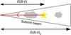 |
Fig. 1 Instrumental-beam and line-of-sight components affecting the comparison of polarized emission with interstellar polarization from differential extinction of a star. E(B − V) is the colour excess to the star, while E(B − V)S is the submillimetre optical depth converted to a colour excess (Sect. 3.3). |
A second condition is purely geometrical, as shown schematically in Fig. 1. In the visible, interstellar polarization and extinction arise from dust averaged over the angular diameter of the star, which is tiny compared to the Planck beam. Furthermore, these observations in the visible probe the ISM only up to the distance of the star, while submillimetre observations probe the whole line of sight through the Galaxy, thus including a contribution from any background ISM (see Fig. 1). As will be discussed below, the effects of these differences can be mitigated and assessed.
As discussed in Sect. 1, current models of interstellar dust commonly feature multiple grain components and not all components (even those that are in thermal equilibrium with the interstellar radiation field and are the major contributors to extinction in the visible and emission in the submillimetre) might be aspherical and aligned. Both the total submillimetre emission, IS, and the optical depth to the star in the V band, τV, entail the full complexity from the contributions of aligned and non-aligned grain populations. while the polarized emission, PS, and the degree of polarization toward the star, pV, isolate properties of the polarizing grains alone.
Because many of the factors driving interstellar polarization, like grain shape, alignment efficiency, and magnetic field orientation, affect pV and PS in similar ways (Martin 2007), we are motivated to examine two polarization ratios, 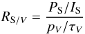 (1)and
 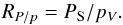 (2)RS /V is the ratio of the polarization fractions at 353 GHz and in the V band. It is a non-dimensional quantity where both numerator and denominator are themselves non-dimensional ratios that apply to the same geometry (common beam and common portion of the line of sight). Furthermore, by virtue of the normalization both PS/IS and pV/τV, the submillimetre and visible polarization fractions, do not depend on the column density and become less sensitive to various factors like the size distribution, grain heating, and opacity that affect the numerator and denominator in similar ways (Martin 2007). RS /V is therefore a robust tool for the data analysis. Being a mix of aligned and non-aligned grains properties2, RS /V is however complex to interpret.
RP/pcharacterizes the aligned grains alone, addressing how efficient they are at producing polarized submillimetre emission compared to their ability at polarizing starlight in the V band. It has the units of polarized intensity, here MJy sr-1. It is easier to interpret, and model, than RS /V. As a drawback, it is less robust than RS /V from the data analysis point of view. Although PS and pV both depend on column density, RP/p is more sensitive to the above geometrical effects and particular attention must be paid to avoid lines of sight with significant background emission. Through PS, RP/p is also directly dependent on the submillimetre emissivity of the polarizing grains and on the intensity of the interstellar radiation field. Nevertheless, RP/p can provide even stronger constraints on the aligned grains than RS /V can.
Despite the overall complexity of the production of dust polarization, studying polarization ratios like RS /V and RP/p provide new insight on some dust properties like optical constants alone. As a corollary, the correlation analysis involving data in the submillimetre and visible for the same line of sight does not provide any information on the dust alignment efficiency.
3. Observations of polarized thermal emission from dust
3.1. Planck data
The Planck HFI 353 GHz polarization maps that we used for the Stokes parameters QS and US (Planck Collaboration Int. XIX 2015) were those from the full mission with five full-sky surveys. These have been generated in exactly the same manner as the data publicly released in March 2013 and described in Planck Collaboration I (2014) and associated papers3.
Intercalibration uncertainties between HFI polarization-sensitive bolometers and differences in bolometer spectral transmissions introduce a leakage from intensity I into polarization Q and U, the main source of systematic errors (Planck Collaboration VI 2014). The Q and U maps were corrected for this leakage (Planck Collaboration Int. XIX 2015)4.
At 353 GHz the dispersion arising from CMB polarization anisotropies is much lower than the instrumental noise for QS and US (Planck Collaboration VI 2014) and so has a negligible impact on our analysis (see Appendix C.2). The cosmic infrared background (CIB) was assumed to be unpolarized (Planck Collaboration Int. XIX 2015).
For the intensity of thermal emission from Galactic dust, IS, we begin with the corresponding Planck HFI 353 GHz map I353 from the same five-survey internal release, corrected for the CMB dipole. From a Galactic standpoint, I353 contains small amounts of contamination from the CMB, the CIB, and zodiacal dust emission. Models for the CMB fluctuations (using SMICA; Planck Collaboration XII 2014) and zodiacal emission (Planck Collaboration XIV 2014) were removed. For this study of Galactic dust emission we subtract the derived zero offset from the map, which effectively removes the CIB monopole (Planck Collaboration XI 2014). The level of the CIB fluctuations (the anisotropies), estimated by Planck Collaboration XI (2014) to be 0.016 MJy sr-1, introduces this uncertainty in IS.
To increase the S/N of the Planck HFI measurements on lines of sight to the target stars (Sect. 4), especially in the diffuse ISM, the Stokes parameters IS, QS, and US, were smoothed with a Gaussian centred on the star, and the corresponding noise covariance matrix was calculated (see Appendix A of Planck Collaboration Int. XIX 2015 for details). The Planck HFI 353 GHz maps have a native resolution of 5′ and a HEALPix5 (Gorski et al. 2005) grid pixelization corresponding to Nside = 2048. Smoothing the Planck data accentuates the beam difference relative to the stellar probe (Fig. 1). Therefore, there is a compromise between achieving higher S/N and maintaining high resolution. The original S/N, and thus any compromise, depends on the region being studied. However, for simplicity we adopted a common Gaussian smoothing kernel, with a full width at half maximum (FWHM) of 5′ (the effective beam is then 7′), and explored the robustness of our results using different choices (Appendix C.2).
3.2. Position angle in polarized emission
The orientation of the plane of vibration of the electric vector of the polarized radiation is described by a position angle with respect to north, here in the Galactic coordinate system. North corresponds to positive Q. In HEALPix, the native coordinate system of Planck, the position angle increases to the west, whereas in the IAU convention the position angle increases to the east; this implies opposite sign conventions for U (Planck Collaboration Int. XIX 2015). In this paper, all position angles, whether ψS in the submillimetre or ψV in the visible, are given in the IAU coordinate system to follow the use in the ISM literature.
On the other hand, all Stokes parameters, whether PlanckQS, US in the submillimetre or qV, uV derived in the visible, are in the HEALPix convention. This accounts for the minus sign both in Eq. (3) and in its inverse form, Eq. (4) below.
Thus from the Planck data we find ![Mathematical equation: \begin{equation} \Gem = \frac{1}{2} \, \arctan(-\usub,\qsub) \,\in [-90\deg,90\deg]. \label{Eq-Gem} \end{equation}](/articles/aa/full_html/2015/04/aa24087-14/aa24087-14-eq40.png) (3)To recover the correct full range of position angles (either [ 0°,180° ], or [−90°,90° ] as used for ψS here) attention must be paid to the signs of both US and QS, not just of their ratio. This is emphasized explicitly by use of the two-parameter arctan function, rather than arctan(−US/QS).
(3)To recover the correct full range of position angles (either [ 0°,180° ], or [−90°,90° ] as used for ψS here) attention must be paid to the signs of both US and QS, not just of their ratio. This is emphasized explicitly by use of the two-parameter arctan function, rather than arctan(−US/QS).
3.3. Column density of the ISM from Planck
A standard measure of the column density of dust to a star from data in the visible is the colour excess E(B − V). An estimate of the column density observed by Planck in the submillimetre is needed to check for the presence of a significant background beyond the star (Fig. 1). This independent estimate was based on the Planck map of the dust optical depth τS (and its error) at 353 GHz, at a resolution of 5′, plus a calibration of τS into an equivalent reddening E(B − V)S, using quasars: E(B − V)S ≃ 1.49 × 10⁴τS (Planck Collaboration XI 2014).
Based on the dispersion of the calibration, and the cross-checks with ancillary data, our adopted estimate for E(B − V)S should be accurate to about 30% for an individual line of sight. We note that this uncertainty is not propagated directly into the final polarization ratios because E(B − V)S is not used in those calculations, but only for selection purposes (Sect. 5.3), whose robustness is explored in Appendix C.
4. Observations of polarization and extinction of starlight
Measurements of stellar polarization, here in the V band, are usually reported in terms of the degree of polarization, pV, and the position angle, ψV, from which we can recover a representation of the observables in the HEALPix convention: 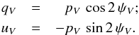 (4)We used the Heiles (2000) catalogue of polarization in the visible, a compilation of several others (e.g., Mathewson & Ford 1971; Mathewson et al. 1978). This catalogue provides pV and its uncertainty σpV, together with ψV ∈ [ 0°,180° ] in the IAU Galactic convention for 9286 stars. For data with S/N> 3, as will be imposed below, it is reasonable to use the Serkowski et al. (1975) approximation to the uncertainty σψV in ψV:
  (5)(e.g., Naghizadeh-Khouei & Clarke 1993). The catalogue also provides an estimate of the distance and colour excess to the star. However, the colour excess has too low a precision (0.1 mag) to be used here.
Accurate extinction data are needed both for the selection of stars (see Sect. 3.3) and for the calculation of RS /V (but not RP/p). We selected stars from various catalogues (Savage et al. 1985; Wegner 2002, 2003; Valencic et al. 2004; Fitzpatrick & Massa 2007) sequentially according to the accuracy of the technique used to derive the colour excess E(B − V). In the shorthand notation of Appendix B, in which there is a description of these catalogues together with our own derivation of E(B − V) for remaining stars using the catalogue of Kharchenko & Roeser (2009), the precedence is FM07, VA04, WE23, SA85, and KR09.
By definition, the optical depth is  (6)The extinction AV is found from E(B − V) through multiplication by the ratio of total to selective extinction, RV = AV/E(B − V), either estimated from the shape of the multifrequency extinction curve or adopted as 3.1 as for the diffuse ISM (e.g., Fitzpatrick 2004) when such a measure is missing. We note that τV is not needed for RP/p.
5. Selection of stars
For each sample, we determined the subsample of stars to be used to calculate the polarization ratios RS /V and RP/p by applying four (sets of) selection criteria. We evaluate the dependence of our results on these criteria in Appendix C.
5.1. S/N
The first criterion was to require a S/N higher than 3 for PS and pV, which propagates into an uncertainty in the position angle of less than 10° (Eq. (5)). We also imposed a S/N higher than three for AV (and consequently, τV), a quantity that might otherwise be poorly estimated6. In emission, this condition is always met automatically for IS when it is required for PS.
Lines of sight where the column density is very low are too noisy in total extinction and in polarized emission to be used with confidence. We therefore also imposed E(B − V) > 0.15 and E(B − V)S> 0.15. The latter criterion ensures that any uncertainties in the small corrections of I353 to IS (Sect. 3.1) are unimportant.
5.2. Diffuse ISM
Our intent is to characterize dust polarization properties in the diffuse, largely atomic, ISM. The column density measure E(B − V)S can be used statistically as a selection criterion: the higher E(B − V)S, the higher the probability of sampling dense environments. We found the selection  (7)(
(7)( ) to be a good compromise between the size of the selected sample and the exclusion of dense environments (which are also generally characterized by a lower dust temperature,
  K).
K).
As one consistency check, we note that the selected lines of sight have low WCO (less than about 2 K km s-1) as judged from the Planck “type 3” CO map (Planck Collaboration XIII 2014) smoothed to 30′ resolution. As another, adopting the average opacity σe(353) = τ353/NH found by Planck Collaboration XI (2014) over the range  (or equivalently
  in units of 1021 cm-2 using the diffuse ISM conversion between E(B − V) and NH from Bohlin et al. 1978) together with this diffuse ISM conversion, we find a consistent calibration between E(B − V)S and τS. Furthermore, Planck Collaboration XI (2014) show that over the above range E(B − V)S compares favourably to estimates of colour excess based on stellar colours in the 2MASS data base (Skrutskie et al. 2006).
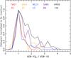 |
Fig. 2 Normalized histograms of the column density ratio RτS for those lines of sight passing the first two selection criteria for S / N and diffuse ISM, for the independent FM07 (red), VA04 (orange), WE23 (blue), SA85 (mauve), and KR09 (black) samples. The number of stars in each sample is indicated. |
5.3. Compatibility between the column densities in the submillimetre and the visible
The selection on E(B − V)S helps to remove some lines of sight with potential emission background beyond the star. This can be supplemented by comparing the PlanckE(B − V)S with E(B − V) for the star (see Fig. 1). Significant disagreement between the two column density estimates, whether an effect of different beams or an effect of the medium beyond the star, would mean that the polarization data cannot be compared usefully. The effect of slightly mismatched columns is mitigated somewhat by the normalization in RS /V, which is a ratio of ratios; it is of heightened concern for RP/p.
We define the column density ratio between the submillimetre and the visible:  (8)Figure 2 presents such a comparison in the form of a normalized histogram of RτS for each sample. For the FM07, VA04, and WE23 samples the histograms correspond to what we would expect for lines of sight with little emission background beyond the star, namely a peak near RτS ≃ 1, and we take this as a first indication of the good quality of the E(B − V)S and E(B − V) estimates. In Sect. 3.3 we estimated that for a given line of sight E(B − V)S might have a 30% uncertainty and from the S/N criterion on τV (Sect. 5.1) the uncertainty in E(B − V) is less than 33%. These uncertainties would readily account for the width of the distribution about this peak.
Nevertheless, the SA85 and KR09 samples are not so well peaked, containing many lines of sight with  . This might indicate a significant background beyond the star, which must in principle arise for some lines of sight. The stars in these independent samples, absent from the other more accurate samples, probe regions of the sky not represented by the other samples. Alternatively, for some lines of sight the dust opacity might be higher than for the diffuse ISM adopted here to derive E(B − V)S (see, e.g., Martin et al. 2012; Roy et al. 2013), leading to an overestimation.
Whatever the reason for this disagreement between E(B − V)S and E(B − V), we need to be wary about including lines of sight with high RτS in our analysis. Therefore, as a third criterion we removed all lines of sight with RτS higher than a certain threshold.
To determine this threshold, we made use of the histograms of the difference in position angles in emission and in extinction: ![Mathematical equation: \begin{equation} \label{deltapsi} \DiffG \equiv \frac{1}{2} \, \arctan{\left[\left(\usub\,\qv - \qsub\,\uv \right),-\left(\qsub\,\qv+\usub\,\uv\right)\right]} . \end{equation}](/articles/aa/full_html/2015/04/aa24087-14/aa24087-14-eq76.png) (9)In the ideal case where measurements of emission and extinction probe the same medium, the polarization directions measured in extinction and in emission should be orthogonal (e.g., Martin 2007). With Eq. (9), orthogonality corresponds to ψS /V = 0°7. Because the systematic presence of backgrounds beyond the stars would induce some deviations from orthogonality, we expect a decline of the quality of position angle agreement as RτS increases.
(9)In the ideal case where measurements of emission and extinction probe the same medium, the polarization directions measured in extinction and in emission should be orthogonal (e.g., Martin 2007). With Eq. (9), orthogonality corresponds to ψS /V = 0°7. Because the systematic presence of backgrounds beyond the stars would induce some deviations from orthogonality, we expect a decline of the quality of position angle agreement as RτS increases.
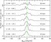 |
Fig. 3 Histograms of difference in position angles ψS /V for successive ranges in column density ratio, RτS, as indicated on the left, with the corresponding number of stars on the right. Only lines of sight of our five samples satisfying the first (S/N) and second (diffuse ISM) selection criteria have been used. For clarity, the histogram has been shifted upward by 10 units for each range. |
This hypothesis is tested in Fig. 3, for lines of sight selected by only the first two criteria (S / N and diffuse ISM). The form of the histogram is observed to depend on the range considered for the column density ratio, RτS. When the column densities agree (RτS ≃ 1), the histogram of ψS /V is well peaked around zero, as expected. This agreement persists as long as RτS is not too large, here below 1.6. Whether we correct for leakage (Sect. 3.1) or not has no effect on these conclusions. As a corollary, the agreement of column densities appears to be a good indicator of consistency between position angles, at least statistically.
Based on this discussion of Figs. 2 and 3, we defined our third selection criterion to be  (10)An alternative way to select lines of sight with little background would be to select according Galactic height or sufficient distance using the Hipparcos catalogue. Although we did not adopt this as an additional criterion, we tested its impact in Appendix C.1.
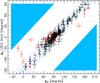 |
Fig. 4 Correlation plot of position angles in emission, ψS, and in extinction, ψV, for the merged sample, for lines of sight satisfying the first three selection criteria. Data for lines of sight failing the fourth angle criterion are marked in red; those finally selected are in black. The central diagonal solid line indicates perfect agreement (orthogonal polarization pseudo-vectors), and other lines are for offsets of 10° (dashed) and 20° (dotted). We note that when the arithmetic difference in angles falls outside the allowed ± 90° range for ψS (filled zones), the plotted ψV is adjusted by ± 180° (Eq. (9)). |
5.4. Consistency of polarization directions (orthogonality)
The fourth selection criterion is a check for the consistency within the uncertainties of the polarization directions in the visible and in the submillimetre8. We adopt  (11)Figure 4 presents a comparison of the position angles for the sample of 226 stars selected above. As anticipated by the histograms of ψS /V in Fig. 3, some lines of sight (plotted in red) are rejected by this fourth criterion. The outliers in Fig. 4 arise at least in part from systematic errors attributable to the small leakage of intensity into polarization that is imperfectly corrected in the March 2013 internal release of the Planck data (Sect. 3.1). Differing beams and paths probed by measurements in the submillimetre and visible (Fig. 1) can also contribute9.
We note that the final sample (plotted in black) covers a considerable range in position angle, i.e., the sample does not only probe environments where the orientation of the polarization in the visible is close to parallel to the Galactic plane (ψV = 90°, ψS = 0°). We will see in the following section that this dynamic range is essential for deriving the polarization ratios RS /V and RP/p using correlation analysis.
5.5. Selected sample of stars
Combining the four sets of criteria (regarding the S/N, the diffuse ISM, the agreement in column densities, and the consistency of position angles) for each sample we selected those lines of sight that would be suitable for a comparison of polarization in the diffuse ISM. Table 1 presents the numbers of stars remaining in our sample after the selection criteria were applied in sequence. Starting from 9286 stars, we retain only 206. We assess the impact of this systematic reduction in Appendix C by relaxing our selection criteria. Our full sample is spread between the different catalogues, thus avoiding any strong dependence on any one in particular.
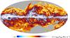 |
Fig. 5 Galactic lines of sight selected in our five independent samples: FM07 (squares), VA04 (asterisks), WE23 (diamonds), SA85 (crosses), and KR09 (triangles). The background image is of debiased polarized intensity, PS, at a resolution of 1° (Planck Collaboration Int. XIX 2015) in a Mollweide projection centred on the Galactic centre. Near Galactic coordinates ( |


Evolution of the number of stars remaining after successive selection criteria are applied.
Figure 5 presents the Galactic coordinates of our selected stars in the five independent samples. Stars are more concentrated in some local ISM regions of interest where the polarization fraction in the submillimetre is known to be high (Planck Collaboration Int. XIX 2015), in particular the Auriga-Fan region around l = 135° and b = − 5° (accounting for about one third of our sample, see Table C.2), the Aquila Rift around l = 20° and b = 20°, and the Ara region at l = 330° and b = − 5°. The fact that all extinction catalogues provide data in these regions allows us to study local variations of RS /V with a limited bias (see Appendix C.3).
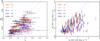 |
Fig. 6 Scatterplots of data for the selected lines of sight (Left: extinction; Right: submillimetre emission). Polarization degree pV and intensity PS were debiased with the Modified Asymptotic method (Plaszczynski et al. 2014). We note the variable that has the larger error in each plot: in the visible, τV (x axis); in the submillimetre, PS (y axis). In the left panel, the line (blue) represents the “classical” upper envelope, pV = 0.0315 τV (Serkowski et al. 1975). This upper envelope has been transferred to the right panel using the derived value for RS /V. |
Figure 6 shows scatterplots of the data for the selected lines of sight. The similar distributions are discussed in Appendix D in the context of RS /V and its relationship to the maximum observed polarization fractions indicated by the envelopes shown. Contributing factors leading to a polarization fraction below the upper envelope(s) include dust grains being less aspherical, a lower grain alignment efficiency, and a suboptimal orientation of the magnetic field with respect to the line of sight (either systemic from viewing geometry or through changes of field orientation along the line sight). None of these factors is addressed by the selection criteria, resulting in a rather diverse set of lines of sight as shown in these scatterplots.
6. Estimates of the polarization ratios
The polarization ratios, RS /V and RP/p, defined in Eqs. (1) and (2), respectively, can in principle be obtained by correlating PS with pV and PS/IS with pV/τV, respectively. However, both the submillimetre polarized intensity,  , and the polarization degree, pV, are derived non-linearly from the original data, the Stokes parameters. In the presence of errors, these are biased estimates of the true values (Serkowski 1958; Wardle & Kronberg 1974; Simmons & Stewart 1985; see also Quinn 2012; Plaszczynski et al. 2014; Planck Collaboration Int. XIX 2015 and references therein). The polarization ratio, RP/p, and the polarization fractions PS/IS and pV/τV – thus also the polarization ratio, RS /V – would be affected by the same problem. We revisit this in Appendix C.4, but use the original data here.
6.1. Correlation plots in Q and U for an unbiased estimate
In the ideal case where noise is negligible and the polarization pseudo-vectors in extinction and emission are orthogonal, from Eqs. (3) and (4) we have10QS/PS = − qV/pV and US/PS = − uV/pV, which yields 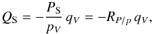 (12)and the same for U. Introducing IS and τV in the denominator on the left and right, respectively, and rearranging slightly, we obtain similarly
 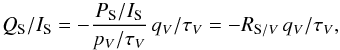 (13)and the same for U. Therefore, the polarization ratios can be measured not only by correlating PS with pV and PS/IS with pV/τV, but also by correlating their projections in Q and U.
We correlate in Q and U first separately, and then jointly. This approach has several advantages. First, while PS, pV, PS/IS and pV/τV are biased, their equivalents in Q and U are not biased11.
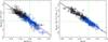 |
Fig. 7 Left: correlation of polarization fractions in emission with those in extinction for the joint fit in Q (black) and U (blue). Using Eq. (15) the best linear fit (red line) has slope and y-intercept − 4.13 ± 0.06 and 0.0006 ± 0.0007, respectively. The Pearson correlation coefficient is − 0.93 and |


Second, the data in Q and U each present a better dynamic range than in P, because they can be both positive and negative and because they can vary from line of sight to line of sight if the position angle ψ changes, even while P and p (or equivalently P/I or p/τ) remain fairly constant. This allows for a better definition of the correlation12 and hence a better constraint on the slope, i.e., the polarization ratio.
Third, we can obtain two independent estimates of the polarization ratios from the slope of separate correlations for Q and for U. Under our hypothesis that for the samples of stars being selected the measured polarization in emission and extinction arises from the same aligned grains, these two estimates of the polarization ratio ought to be the same and the intercepts ought to be close to zero. This is what we find. For the Q and U independent correlations analyzed using the scalar equivalent of Eq. (15) the slopes of the RS /V fit are, respectively, − 3.90 ± 0.09 and − 4.03 ± 0.14 and the y-intercepts are 0.0060 ± 0.0010 and − 0.0014 ± 0.0009. For the RP/p fit, the slopes are (− 5.17 ± 0.09) MJy sr-1 and (− 5.07 ± 0.13) MJy sr-1 and the y-intercepts are (0.0077 ± 0.0013) MJy sr-1 and (− 0.0016 ± 0.0013) MJy sr-1. In both cases the y-intercepts are small compared to the dynamic range in Q and U (see Fig. 7). The uncertainties quoted were derived in the standard way from the quality of the fit. As reinforced by our bootstrapping analysis below (Sect. 6.2), the results of these independent fits are compatible with our hypothesis that the two correlations are measuring the same phenomenon, and furthermore reflect the quality of the selected data. See also Appendix C.4 for a comparison with the fits in P.
Fourth, given this satisfactory consistency check, measuring the polarization ratios from the correlation of the joint data (Q,U) is both motivated and justified. We compute the linear (y = ax + b) best fit to the data by minimizing a χ2, which for the joint fit has the form13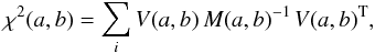 (14)with
 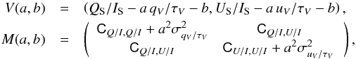 (15)for the RS /V fit, and
 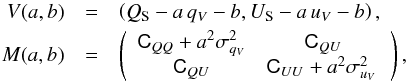 (16)for the RP/p fit. The calculation of the elements C of the noise covariance matrix, [ C ], for the Planck data is presented in Appendix A. The slopes of the joint correlation are − 4.13 ± 0.06 and (− 5.32 ± 0.06) MJy sr-1, respectively.
Figure 7 shows that the joint correlations are remarkably tight.The Pearson correlation coefficients are − 0.93 for RS /V and − 0.95 for RP/p. Values of the reduced χ2 of the fit ( for RS /V and 2.29 for RP/p) are higher than expected given the large number of degrees of freedom (410), in part because the noise covariance matrix does not capture the systematic errors in the data, primarily from the leakage correction (see Sect. 3.1). Nevertheless, the tight correlation in Fig. 7 is in sharp contrast to the scatter among the underlying observables in Fig. 6. The contributing factors that move points below the upper envelopes in Fig. 6 move points toward the origin along the relevant visible (horizontal) and submillimetre (vertical) axes in Fig. 7, left, and actually along the correlation line toward the origin if the changes in the submillimetre and visible polarization fractions are related by the same RS /V for all lines of sight, as they evidently are. Similar comments apply to Fig. 7, right. As a complement, we show in Appendix D that a statistical analysis of the maximum polarization fractions seen in the visible and at 353 GHz gives a result consistent with RS /V.
These good correlations confirm our initial idea that the polarization ratios can be obtained without limiting the analysis to the case of optimal alignment (magnetic field in the plane of the sky, perfect alignment), and that the dependences of polarization on the magnetic field orientation and on the dust alignment efficiency are similar in emission and in extinction. We conclude that RS /V and RP/p are each characterizing a property of the dust populations that is homogeneous across a diverse set of lines of sight in the diffuse ISM.
6.2. Mean values and uncertainties for RS/V and RP/p in the diffuse ISM
Because of the finite sample size and potential sensitivity to the exact membership in the samples, we used the technique of bootstrapping (Efron & Tibshirani 1993), in particular random sampling with replacement or case resampling, to carry out many instances of the fit, and then from these solutions we calculated the mean slope, the mean intercept, and their dispersions. The number of trials, 500, was large enough to ensure convergence of the results of resampling.
For all of the fits – RS /V and RP/p and Q, U, and joint – we find the same slopes using bootstrapping as we found in the direct fits. The uncertainties are somewhat more conservative, by up to a factor of 4 for Q. In the rest of this paper we report the results from bootstrapping in terms of RS /V and RP/p (the negative of the values of the slopes) and to be conservative the dispersions were rounded to the upper first decimal (e.g., 0.12 gives 0.2) to give the statistical uncertainties quoted below.
In Appendix C we investigatedthe robustness of the polarization ratios RS /V and RP/p with respect to the selection criteria defining the sample, the data used, the region analyzed, and the methodology. We derived each time the mean values and uncertainties of the polarization ratios. We showed that all systematic variations of RS /V and RP/p are small, less than twice the statistical uncertainty derived from the fit.
On the basis of these results we adopt  (17)This appears to be a homogeneous characterization of diverse lines of sight in the diffuse ISM. The statistical uncertainty is representative of the standard deviation of the histogram of RS /V found by bootstrap analysis in the many robustness tests (Appendix C). The systematic error gathers all potential contributions, but is dominated by our incomplete knowledge of the small correction of Planck data for leakage of intensity into polarization (Sect. 3.1).
For the other polarization ratio we adopt ![Mathematical equation: \begin{equation} \ratiop=\psub / \pv = \left[\resrp\pm\ressp\ (\stat)\pm\resspcombined\ (\sys)\right]\,{\rm MJy\,sr^{-1}}. \end{equation}](/articles/aa/full_html/2015/04/aa24087-14/aa24087-14-eq144.png) (18)The statistical uncertainty from the bootstrap analyses is again rather small. Uncertainties in RP/p are dominated by systematic errors, namely from uncertainties in the leakage correction and from the tendency to overestimate RP/p in the presence of backgrounds beyond the stars.
(18)The statistical uncertainty from the bootstrap analyses is again rather small. Uncertainties in RP/p are dominated by systematic errors, namely from uncertainties in the leakage correction and from the tendency to overestimate RP/p in the presence of backgrounds beyond the stars.
The corresponding total intensity per unit magnitude in the V band, IS/AV, is obtained by the direct calculation IS/AV = RP/p/RS /V/ 1.086 = 1.2 MJy sr-1, with an uncertainty ± 0.1 MJy sr-1.
To help in constraining dust models, we provide the mean SED for the lines of sight in our sample in the form of a modified blackbody fit to the data (Planck Collaboration XI 2014): Tdust = 18.9 K; βFIR = 1.62; and a dust opacity at 353 GHz, τS/AV = 2.5 × 10⁻⁵ mag-1.
7. Discussion
Our measurement of the polarization ratios RS /V and RP/p provide new constraints on the submillimetre properties of dust. In fact, in anticipation of results from Planck, RS /V for the diffuse ISM has already been predicted in two studies.
7.1. RS/V from dust models
Martin (2007) discussed how PS/IS at 350 GHz can be predicted by making use of what is already well known from dust models of visible (and infrared and ultraviolet) interstellar polarization and extinction. From that study, the polarization ratio of interest here, RS /V, can be recovered by dividing the estimated values of PS/IS in the last row of his Table 2, first by 100 (to convert from percentages) and then by 0.0267, the value of pV/τV on which the table was based. For example, for aligned silicates in the form of spheroids of axial ratio 1.4, the entry is 9.3, so that RS /V = 3.5. Similar values are obtained for other shapes and axial ratios, because changes in these factors affect polarization in both the visible and submillimetre. Sources of uncertainty in this prediction include: whether imperfect alignment reduces the polarization equally in the visible and submillimetre (as was assumed); how the extinction in the visible including contributions by unaligned grains, is modelled, whether by aligned or by randomly oriented grains (± 25%); and the amount by which the submillimetre polarization fraction is diluted by unpolarized emission from carbonaceous grains in the model (adopting a dilution closer to that in the Draine & Fraisse (2009) mixture discussed below could raise RS /V to about 4.5).
Draine & Fraisse (2009) also made predictions of PS/IS for mixtures of silicate and carbonaceous grains, where again the dust model parameters (size distributions, composition, alignment, etc.) were constrained by a detailed match to the infrared to ultraviolet extinction and polarization curves, with the normalization pV/τV = 0.0326. According to their Fig. 8, at 350 GHz PS/IS is about 13–14% for models in which only the silicate grains are aspherical and aligned (axial ratio 1.4–1.6)14, and about 9–10% for models in which both silicate and carbonaceous grains are aspherical and aligned. Dividing as above yields RS /V = 4.1 and 2.9, respectively.
These are challenging calculations that encounter similar issues to those discussed in Martin (2007). Given the uncertainties, we conclude that the predictions of RS /V are in reasonable agreement with what has now been observed, providing empirical validation of many of the common basic assumptions underlying polarizing grain models. Although validating the basic tenets of the models, the new empirical results on RS /V do not allow a choice between different models.
7.2. RP/p and IS/AV from dust models
The polarization ratio RP/p is a more direct and easier-to-model observational constraint. Unlike for RS /V, one does not need to model the extinction and emission of non-aligned or spherical grain populations. Model predictions for RP/p will depend not only on the size distribution, optical properties, and shape of the aligned grain population, but also on the radiation field intensity through the dependence of PS on the grain temperature.Because RP/p is not a dimensionless quantity like RS /V, it provides a new constraint on grain models, i.e., models that are able to reproduce RS /V will not automatically satisfy RP/p.
From the Draine & Fraisse (2009) prediction of PS/NH we measure νSPS/NH ≃ 1.0 × 10⁻¹¹ W sr-1 per H at 353 GHz. In the visible the same models produce pV/NH ≃ 1.4 × 10⁻²³ cm2 per H (their Fig. 6, taking into account their Erratum). These can be combined to give RP/p ≃ 2.2 MJy sr-1. Our empirical results are significantly higher, by a factor of 2.5, and so represent a considerable challenge to these first polarizing grain models. A basic conclusion is that the optical properties of the materials in the model need to be adjusted so that the grains are more emissive.
As this example illustrates, there is great diagnostic power in focusing directly on the polarization properties alone; RP/p describes the aligned grain population and so is important, along with RS /V, for constraining and understanding the full complexity of grain models.
Complementing the discussion in Sect. 7.1, from the Draine & Fraisse (2009) prediction of IS/NH we measure νSIS/NH ≃ 0.7–1.1 × 10⁻¹⁰ W sr-1 per H at 353 GHz. In the visible the same models produce τV/NH ≃ 4.5 × 10⁻²² cm2 per H (their Fig. 4). These can be combined to give IS/τV ≃ 0.5–0.8 MJy sr-1, after a colour correction by 10%, taking into account the width of the 353 GHz Planck band (Planck Collaboration IX 2014). Our empirical results are significantly higher than these models, by a factor of 1.5–2.4, depending on the model15. Again, this is in the sense that the grains need to be more emissive, though the magnitude of the discrepancy is somewhat lower than it is for polarized emission.
8. Conclusion
Comparison of submillimetre polarization, as seen by Planck at 353 GHz, with interstellar polarization, as measured in the visible, has allowed us to provide new constraints relevant to dust models for the diffuse ISM. After carefully selecting lines of sight in the diffuse ISM suitable for this comparison, a correlation analysis showed that the mean polarization ratio, defined as the ratio between the polarization fractions in the submillimetre and the visible, is  (19)where the statistical uncertainty is from the bootstrap analysis (Sect. 6.2) and the systematic error is dominated (Appendix C.2) by our incomplete knowledge of the small correction of Planck data for leakage of intensity into polarization (Sect. 3.1).
Similarly we found the ratio between the polarized intensity in the submillimetre and the degree of polarization in the visible: ![Mathematical equation: \begin{equation} \label{ratioPsummary} \ratiop= \psub / \pv=\left[\resrp\pm\ressp\ (\stat)\pm\resspcombined\ (\sys)\right]\,{\rm MJy\,sr^{-1}}. \end{equation}](/articles/aa/full_html/2015/04/aa24087-14/aa24087-14-eq171.png) (20)This analysis using the new Planck polarization data suggests that the measured RS /V is compatible with a range of polarizing dust models, validating the basic assumptions, but not yet very discriminating among them. By contrast, the measured RP/p is higher than model predictions by a factor of about 2.5. To rectify this in the dust models, changes will be needed in the optical properties of the materials making up the large polarizing grains that are emitting in thermal equilibrium.Thus, the simpler polarization ratio RP/p turns out to provide a more stringent constraint on dust models than RS /V.
(20)This analysis using the new Planck polarization data suggests that the measured RS /V is compatible with a range of polarizing dust models, validating the basic assumptions, but not yet very discriminating among them. By contrast, the measured RP/p is higher than model predictions by a factor of about 2.5. To rectify this in the dust models, changes will be needed in the optical properties of the materials making up the large polarizing grains that are emitting in thermal equilibrium.Thus, the simpler polarization ratio RP/p turns out to provide a more stringent constraint on dust models than RS /V.
Future dust models are needed that will satisfy the constraints provided by both RS /V and RP/p, as well as by the spectral dependencies of polarization in both the visible and submillimetre. How the optical properties of the aligned grain population (including the silicates) should be revised in the submillimetre and/or visible needs to be investigated through such detailed modeling.Understanding the polarized intensity from thermal dust will be important in refining the separation of this contamination of the CMB.
Online material
Appendix A: Uncertainties for polarization quantities
We start with the values of the Stokes parameters, I, Q, and U, and the noise covariance matrix, [ C ], at the position of each star. By definition, the uncertainties σQS of QS and σUS of US are calculated from the variances  and
and  , respectively.
The variance of the polarized intensity  (without bias correction) is
  (A.1)from which we derive the S / N of the polarization intensity, P/σP. For the uncertainty in the position angle ψS we use the approximate formula in Eq. (5), which is appropriate because we always require the S/N to be larger than 316.
The uncertainty of the projected polarization fraction QS/IS has the following dependence:  (A.2)and the same holds for US/IS. The covariance of QS/IS with US/IS follows:
  (A.3)The uncertainties σQS/IS and σUS/IS, used for plotting only, are derived simply from the variances CQ/I,Q/I and CU/I,U/I.
When the data are smoothed, with the method described in Appendix A of Planck Collaboration Int. XIX (2015)17, the formulae hold substituting the smoothed Stokes parameters and the elements of the corresponding covariance matrix, [].
Appendix B: Extinction catalogues
Appendix B.1: Extinction and colour excess catalogues
Using stellar atmosphere models, Fitzpatrick & Massa (2007) provide well-determined E(B − V) and AV measurements for 328 stars, 14 of which could be identified in the Heiles (2000) polarization catalogue via their catalogue identifiers (HD – Henry Draper, BD – Bonner Durchmusterung, CD – Cordoba Durchmusterung, or CPD – Cape Photographic Durchmusterung identifiers). This was the basis for what we refer to as the “FM07 sample”. Similarly, from the Valencic et al. (2004) and Wegner (2002, 2003) extinction catalogues (derived with the more standard technique based on “unreddened” reference stars), we generated the VA04 and WE23 samples; we note that we have removed stars in common with previously-defined samples, with the same order in priority of the samples. These three samples all contain measurements of both AV and E(B − V), providing an estimate of RV, a useful diagnostic of the diffuse ISM where RV is close to 3.1.
The Savage et al. (1985) catalogue provides measures of E(B − V) to 1415 stars, 1085 of which were identified in the Heiles (2000) catalogue. Lacking a measure of RV, we assumed the standard value for the diffuse ISM, RV = 3.1; its uncertainty δRV = 0.418 adds another uncertainty to our estimate of τV. Again removing stars in common with previous samples, we built the SA85 sample.
Appendix B.2: Deriving E(B–V) from the Kharchenko & Roeser star catalogue
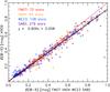 |
Fig. B.1 Correlation between our derived E(B − V) from the Kharchenko & Roeser (2009) catalogue with that for common stars in the FM07, VA04, and WE23 samples. Only data with S / N on E(B − V) larger than 3 are presented. The red line is a 1:1 correlation, while the black line is a fit. |
As described below, using the high-quality photometry in the all-sky catalogue of Kharchenko & Roeser (2009) we were able to derive E(B − V) and its uncertainty for more than 3000 stars present in the Heiles (2000) catalogue. Stars absent from other samples then form the KR09 sample. As for the SA85 catalogue, we assumed RV = 3.1 ± 0.4 for all stars.
The Kharchenko & Roeser (2009) catalogue (SIMBAD reference code I/280 B) used for the derivation of E(B − V) is a compilation of space and ground-based observational data for more than 2.5 million stars. The catalogued data include, among others, B and V magnitudes in the Johnson system, K magnitude, HD number, and the spectral type and luminosity class of the star. TOPCAT19 (Taylor 2005) was used to cross-match the polarization (Heiles 2000) and extinction (Kharchenko & Roeser 2009) catalogues with the HD number as the first-order criterion. Where two or more stars are identified with the same number, the one for which the visual magnitude is closest to that in the polarization catalogue was retained. For the rest of the catalogue, a coordinate-match criterion with a 2′′ radius was applied, using the visual magnitude to choose between candidates if necessary.
We have used the intrinsic colors (B − V)0 derived by Fitzgerald (1970) for different spectral classifications. The colour excess for each of star was calculated according to E(B − V) = (B − V)KR09 − (B − V)0, using the B and V magnitudes and the corresponding intrinsic colour deduced from the spectral classification in the Kharchenko & Roeser (2009) catalogue. Following Savage et al. (1985), Be stars and stars with spectral types B8 and B9 were removed.
A few hundred stars overlapping the FM07, VA04, WE23, or SA85 samples allowed us to check the quality of our derivation of E(B − V). Figure B.1 reveals a good correlation with the other samples, with our KR09 E(B − V) tending to underestimate the reddening to the star by about 9%. This small discrepancy has only a small impact on the derived RS /V (the KR09 sample represents one third of our sample, see Table 1) and does not affect RP/p.
Appendix C: Robustness tests
From the joint fits and bootstrap analysis of uncertainties in Sects. 6.1 and 6.2 we found RS /V = 4.1 ± 0.2 and RP/p = (5.3 ± 0.2) MJy sr-1. In this appendix we investigate the robustness of these polarization ratios with respect to the selection criteria defining the sample, the data used, the region analyzed, and the methodology. We derive each time their mean values and uncertainties.
As a potential drawback owing to its simplicity, RP/p involves systematic dependences on parameters such as the ambient radiation field, the submillimetre opacity of aligned grains, and the presence of a background beyond the star. Because PS and pV are proportional to the column density (of polarizing dust) probed with their respective observations in the submillimetre and visible, the correlation presented in Fig. 7 is potentially biased (an overestimate) if there is systematically a background beyond the stars selected (Fig. 1). Thanks to the normalization of PS by IS and pV by τV, such dependences are weakened20 in the analysis of RS /V.
Appendix C.1: Selection criteria
We explore the effects of varying the limits of the four selection criteria presented in Sect. 5. We do this one criterion at a time, with the others unchanged. We also examine other alternatives for defining the sample.
S/N.
The accuracy of the polarization degree in extinction data is not a limiting factor because the mean S / N is about 10 for the selected stars. Asking for a S / N threshold higher than 3 (Sect. 5.1) for PS and for AV could bias our estimates of RS /V, which is proportional to these quantities. It would also exclude many diffuse regions where such a high S/N cannot be achieved at 5′ resolution. Nevertheless, we find no significant variation of the polarization ratios when imposing S/N> 1 (268 stars, RS /V = 4.1 ± 0.1, RP/p = (5.3 ± 0.2) MJy sr-1) or S/N> 10 (68 stars, RS /V = 4.3 ± 0.2, RP/p = (5.4 ± 0.2) MJy sr-1).
Diffuse ISM.
The E(B − V)S criterion (Eq. (7) in Sect. 5.2) is responsible for the removal of lines of sight toward denser environments or toward the Galactic plane. Ignoring this criterion so that these stars are included gives RS /V = 4.0 ± 0.2 and RP/p = (5.7 ± 0.2) MJy sr-1, for 284 stars. On the other hand, we can be more strict in our selection by imposing lower E(B − V)S. A limit  rather than our reference criterion 0.8 has no effect. With even lower column densities (
 and 0.3), we get RS /V = 4.7 ± 0.2 and RS /V = 4.7 ± 0.4, for 82 and 42 stars, respectively. While an increase in RS /V with decreasing column density could arise through the inverse dependence of RS /V on IS (Eq. (1)), the evidence is not strong. Changes in RP/p are not significant: (5.7 ± 0.2) MJy sr-1 and (5.6 ± 0.4) MJy sr-1, respectively.
We can restrict our sample to lines of sight where the ratio of the total to selective extinction, RV, is close to 3.1, its characteristic value for the diffuse ISM (e.g., Fitzpatrick 2004). Specifically, we exclude those lines of sight where RV was not measured (SA85, KR09), and impose 2.6 <RV< 3.6. Our sample is then reduced to 69 stars and gives RS /V = 4.0 ± 0.2 and RP/p = (5.2 ± 0.2) MJy sr-1.
A similar selection can be made on the basis of the wavelength corresponding to the peak of the polarization curve in extinction, λmax, as taken from Serkowski et al. (1975). Imposing 0.5 μm <λmax< 0.6 μm, we find RS /V = 4.0 ± 0.3 and RP/p = (5.1 ± 0.3) MJy sr-1, for 34 stars.
Column density ratio.
The polarization ratio RS /V is, by construction, proportional to E(B − V) and could therefore anticorrelate with RτS. However, we do not find such dependance when varying the upper limit of RτS from 1.2 (RS /V = 4.2 ± 0.2, 121 stars) to 1.8 (RS /V = 4.1 ± 0.1, 231 stars). Going beyond the limits where angles agree, with upper limits of 2.0 and 3.0, yields the same value 4.1 ± 0.2 for the polarization ratio, for 251 and 284 stars, respectively. We also tested other proxies to estimate the total column density observed by Planck. Replacing the dust optical depth at 353 GHz, used to derive E(B − V)S, by the Hi 21 cm emission or the dust radiance (the total power emitted by dust, Planck Collaboration XI 2014) did not affect our polarization ratios significantly.
Orthogonality.
If we become more restrictive in our selection based on the difference between position angles (Eq. (11) in Sect. 5.4), by requiring a 1σ agreement our sample shrinks to 112 stars. The quality of the fit is preserved, as expected: RS /V = 4.2 ± 0.2 and RP/p = (5.5 ± 0.2) MJy sr-1.
Galactic height.
As mentioned in Sect. 5.3, the Galactic height of the star can play a role, similar to that of the column density ratio RτS, in selecting lines of sight with a low probability of background emission. Still requiring RτS< 1.6 and then selecting on H> 100 pc, H> 150 pc, and H> 200 pc, we find the same polarization ratios, RS /V = 4.1 ± 0.1 for 136, 91 and 53 stars, respectively. Selecting on H> 100 pc without selecting on the column density ratio, we obtain RS /V = 4.0 ± 0.2 (172 stars). Results for RP/p are also similar, with an average RP/p = (5.2 ± 0.1) MJy sr-1.
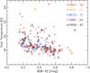 |
Fig. C.1 Planck line of sight dust temperature Tdust (Planck Collaboration XI 2014) and the column density to the star, E(B − V), for the independent samples. |
Thermal dust temperature.
The dust temperature Tdust from Planck Collaboration XI (2014) characterizes the spectral energy distribution of the combined emission IS from all dust components in the column of dust along the line of sight and has no direct connection to the sample selection. Figure C.1 shows the distribution in the Tdust – column density (as measured by E(B − V)) plane. The ranges of E(B − V) and Tdust are considerable for each sample. In this plane, there is a band showing a slight anti-correlation of Tdust and E(B − V); there are also several lines of sight with Tdust ≃ 21 K but with a range of E(B − V).
We looked for any dependencies of RS /V, RP/p, and IS/AV on Tdust, for data with and without the correction for leakage of intensity into polarization. In Fig. C.2 the data were binned in Tdust, each bin containing the same number of stars. The blue curve in the right panel of Fig. C.2 shows the relative change arising from the expected increase in IS (but not AV) when Tdust increases. It has been fit to the data in the vertical direction. A similar trend in RP/p arising from PS would be expected in the middle panel if the subset of grains that are polarizing had the same temperature as characterized the total emission. This appears to be consistent with the corrected data. Under the same hypothesis, the trend for RS /V would be flat in the left panel. This too appears to be consistent with the corrected data.
Appendix C.2: Data used
Here we test the sensitivity of our results to the choice of extinction catalogues and to the smoothing and original processing of the Planck data. The main sources of data uncertainty are, for the extinction data, the measure of AV and, for the polarized emission data, the instrumental systematics related to the correction for the leakage of intensity to polarization (Sect. 3.1).
Extinction catalogues.
One important source of uncertainty in RS /V (not RP/p) is the measure of the dust extinction in the visible, AV. In Table C.1 we summarize our results for each catalogue taken separately, independently of the others (i.e., we do not remove common stars). Although the catalogues neither share all of the same stars nor have the same extinction data for stars in common, the estimates obtained for RS /V and IS/AV are compatible. RP/p is independent of AV, therefore of any extinction samples. Its variations among catalogues helps to constrain its statistical uncertainty, here less than 0.2 MJy sr-1.
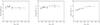 |
Fig. C.2 Left: mean RS /V as a function of the mean Tdust, each plotted with the standard deviation, in bins of equal number. Two versions of the Planck data have been used: with (black) and without (red) correction for leakage of intensity into polarization. Middle: the same, but for RP/p. Right: the same, but for IS/AV. The blue curves, motivated in the right panel, show the expected response of the ratios to an increase in Tdust, according to a simple model in which the subset of grains that are polarizing had the same temperature as characterized the total emission (see text). |
Smoothing.
In order to increase the S / N of the Planck polarization data and increase the quality of the correlations in Q and U, we chose to smooth our maps with a 5′ FWHM Gaussian, making the effective map resolution 7′. Because Q and U are algebraic quantities derived from a polarization pseudo-vector, the smoothing of polarization maps statistically tends to diminish the polarization intensity PS, which would propagate into the polarization ratios RS /V and RP/p. Using the raw (not smoothed) data, or data smoothed with a beam of 3′ and 8′ (keeping the same sample as was selected using data smoothed with a 5′ beam to allow for an unbiased comparison), we find RS /V = 4.0 ± 0.2, 4.1 ± 0.2, 4.2 ± 0.2, and RP/p = (5.2 ± 0.3) MJy sr-1, (5.3 ± 0.2) MJy sr-1, (5.4 ± 0.2) MJy sr-1), respectively.
We note that the mean values of RS /V and RP/p could still be underestimated owing to depolarization in the Planck beam, which does not have a counterpart in the visible measurement (see Fig. 1); however, this effect should be small and within the uncertainties.
Zodiacal emission.
Removing zodiacal emission, or not, in deriving IS (Sect. 3.1) does not affect our result, with RS /V = 4.1 ± 0.2 in both cases.
Contamination by CMB polarization at 353 GHz.
Following the approach in Planck Collaboration Int. XXII (2015), we can remove the CMB patterns in intensity and polarization from the 353 GHz maps by subtracting the 100 GHz (I,Q,U) maps in CMB thermodynamic temperature units. This method unfortunately adds noise to the 353 GHz maps, and is therefore used only as a check. It also has the drawback of subtracting a fraction of dust emission that is present in the 100 GHz channel. However, dust is then subtracted both in intensity and in polarization, though perhaps not proportionally to the polarization fraction at 353 GHz (however, this is a second-order effect). With this 100 GHz-subtracted version of Q and U, we obtain RS /V = 4.1 ± 0.2 and RP/p = (5.2 ± 0.2) MJy sr-1, for 203 stars.
Values of RS /V and RP/p in specific regions.
Leakage correction.
A small correction for leakage of intensity into polarization has been applied to the Planck polarization data used here (see Sect. 3.1). While this correction is imperfect, the alternative of ignoring this correction leaves systematic errors in the data. For the version of the data not corrected for leakage, we obtain figures similar to Fig. 7, for 196 selected stars, with Pearson correlation coefficients − 0.94 and − 0.95 and  and 2.56, for RS /V and RP/p, respectively. Running the bootstrap analysis we find RS /V = 4.3 ± 0.2 and RP/p = (5.5 ± 0.2) MJy sr-1, systematic changes of + 0.2 and + 0.2 MJy sr-1 compared to our values for data corrected for leakage. Therefore, the correction of the March 2013 Planck polarization data for this leakage is a significant source of systematic uncertainty in RS /V and RP/p, though perhaps the uncertainty is not as much as 0.2 or of the same sign.
Appendix C.3: Region analyzed
The polarization ratios that we derived are an average over the sky. Here we examine the ratios for spatial subsets of the data.
Galactic hemisphere or latitude.
We find no significant variation of the polarization ratios between the two hemispheres: RS /V = 4.0 ± 0.3 and RP/p = (5.1 ± 0.3) MJy sr-1 for the northern Galactic hemisphere, and RS /V = 4.2 ± 0.1) and RP/p = (5.4 ± 0.2) MJy sr-1 for the southern.
Polarization ratios might depend on the latitude of stars if that were indicative of different potential backgrounds. Selecting high latitude stars from both hemispheres (| b | > 6°, 95 stars) to limit the presence of backgrounds, we find RS /V = 4.2 ± 0.3, RP/p = (5.2 ± 0.3) MJy sr-1, and IS/AV = (1.24 ± 0.07) MJy sr-1. For low latitude stars ( , 111 stars), RS /V = 4.1 ± 0.1, RP/p = (5.3 ± 0.2) MJy sr-1, and IS/AV = (1.25 ± 0.04) MJy sr-1, with no indication of any contamination by backgrounds.
Selected regions on the sky.
Table C.2 presents the polarization ratios for three regions, among them the Fan which contains almost one third of our selected stars; these results are close to the overall average. If we select all stars except those from the Fan, we find RS /V = 4.2 ± 0.2 and RP/p = (5.4 ± 0.2) MJy sr-1. Table C.2 also presents the polarization ratios for two other regions in the local ISM where stars in our sample are more concentrated (see Fig. 5): the Aquila Rift, and the Ara region (Planck Collaboration Int. XIX 2015). Taking into account the uncertainties, we conclude that our total sample is not biased by any particular region and there is no evidence for spatial variations.
Appendix C.4: Correlation plots in P
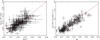 |
Fig. C.3 Left: correlation of debiased polarization fraction in emission with that in extinction (Pearson coefficient 0.74). Right: correlation of the debiased polarized emission (in MJy sr-1) with starlight polarization degree (Pearson coefficient 0.87). The range corresponds to one quadrant in Fig. 7. The fits are forced to go through the origin and have slopes RS /V = 4.18 ± 0.04 ( |


In Sect. 6.1 we derived RS /V and RP/p using joint correlation plots in Q and U rather than in the biased quantity P. However, our selection of PS and pV with S/N> 3 implies that the bias should not be too significant and it is possible to debias P at least statistically (the Modified Asymptotic debiasing method of Plaszczynski et al. 2014 was used; see also references in Sect. 6.1). This is confirmed by the correlation plot in Fig. C.3 for debiased polarization fractions (which are almost identical to those for the original data). The data in the submillimetre and visible show a fairly good correlation, though, compared with Fig. 7, have a smaller dynamic range and a smaller Pearson correlation coefficient. We fit the slopes, forcing the fit to go through the origin unlike for the fits in Fig. 7. Whether with debiased data or not, the polarization ratios (from bootstrapping) are essentially identical: RS /V = 4.2 ± 0.1 and RP/p = (5.4 ± 0.1) MJy sr-1, and also the same as found in the preferred analysis in Fig. 7.
Appendix D: RS/V and its relationship to the maximum observed polarization fractions
For a given dust model, including the grain shape, the maximum polarization fraction that can be observed corresponds to the ideal case of optimal dust alignment: the magnetic field lies in the plane of the sky, has the same orientation (position angle) along the line of sight, and the dust alignment efficiency with respect to the field is perfect. The maximum pV/τV ≃ 3% observed in extinction (corresponding to  , Serkowski et al. 1975), is supposed to be close to this ideal case (Draine & Fraisse 2009).For our selected sample of lines of sight, Fig. 6 (left panel) shows this classical envelope and the corresponding envelope (PS/IS = 3% × RS /V = 12.9%) transferred to emission (right panel).
We have also investigated the upper envelope that might be derived independently from the emission data. At a resolution of 1°Planck HFI has revealed regions with PS/IS greater than 20% (Planck Collaboration Int. XIX 2015), albeit for only a very small fraction (0.001, their Fig. 18) of lines of sight, toward local diffuse clouds. This value, which is already a high envelope, might have been even larger were it at the finer resolution of starlight measurements. Combined with the 3% limit from stars, this would apparently imply RS /V> 6, significantly higher than our mean value RS /V = 4.2.
However, for statistical reasons, these two estimates of RS /V cannot be compared straightforwardly: Planck statistics are based on (almost) full-sky data, while those of Serkowski et al. (1975) are based on less than 300 stars. A more consistent statistical comparison can be sought. Analyzing Fig. 9 of Serkowski et al. (1975) and limiting our analysis to stars
satisfying 0.15 <E(B − V) < 0.8 as in our selection criterion (Sect. 5.2), the upper envelope is approximately the 96% percentile of pV/E(B − V) (in this interval of E(B − V), 8 stars out of about 200 lie above this envelope). The corresponding 96% percentile of PS/IS in our selected sample is PS/IS = 14.5% (8 stars out of 206 above that line). As a complement, we can obtain an estimate of the 96% percentile of the full Planck map by smoothing the 353 GHz maps with a Gaussian of 5′ and selecting those pixels with 0.15 <E(B − V)S< 0.8. The 96% percentile of PS/IS (after debiasing) in this sample of over 107 pixels is found to be 13.2%. Combining these estimates based on consistent percentiles implies RS /V in the range 4.2−4.6, compatible with our direct, and more rigorous, result.
Planck (http://www.esa.int/Planck) is a project of the European Space Agency (ESA) with instruments provided by two scientific consortia funded by ESA member states (in particular the lead countries France and Italy), with contributions from NASA (USA) and telescope reflectors provided by a collaboration between ESA and a scientific consortium led and funded by Denmark.
There are possible contributions by large unaligned grains to the total thermal emission and extinction. These contributions cause a dilution of the polarization fractions.
However, the publicly released data include only temperature (intensity) maps, based on the first two surveys.
The systematic errors that we quote include uncertainties associated with residual systematics as estimated by repeating the analysis on different subsets of the data. We have also checked our data analysis on the latest version of the maps available to the consortium to verify that the results are consistent within the uncertainties quoted in this paper.
For the catalogues where RV was not measured (SA85 and KR09), the assumed uncertainty δRV = 0.4 introduced in Sect. B.1 is ignored in the selection process, but not in the data analysis and fitting.
The expression for ψS /V follows from the arctan addition rule as for Eq. (7) in Planck Collaboration Int. XIX (2015), with a minus sign before each argument allowing for the rotation by 90° of the polarization direction in emission as measured by ψS and an additional sign change in the first argument because ψS /V, like ψS and ψV, follows the IAU convention for angles, increasing from north through east (Eq. (3)).
Consistency of the orientation of polarization in the visible at  resolution with the direction of the interstellar magnetic field inferred from K band (23 GHz) polarization measured by WMAP has been noted by Page et al. (2007). This is of interest whether the K band polarization arises from synchrotron emission or dust. Likewise, in their BICEP millimetre-wave polarization Galactic plane survey in the longitude range 260°<l< 340°, Bierman et al. (2011) found general consistency with polarization angles in the visible.
Planck Collaboration Int. XIX (2015) have found that the dispersion of the position angles measured in neighbouring Planck beams is anti-correlated with PS/IS (their Fig. 23). Dispersions comparable to the angle ψS /V of the outliers in Fig. 4 occur statistically at low PS/IS, below a few percent. We find that ψS /V anti-correlates with PS/IS too, suggesting that the same processes are responsible for the dispersion of the position angles in both extinction and emission at low fractional polarization.
Equation (4) changes the signs of both qV and uV when the position angle ψV is changed by 90°.
Analysis using Q and U makes it possible to skip the S/N criteria for pV and PS, but not for AV and IS, as is explored in Appendix C.1.
The x and y coordinates can be inverted in the fitting routine without affecting the measure of the polarization ratio.
This prediction of 13–14% for PS/IS when graphite grains are spherical is overestimated. As can been seen from Fig. 7 in Draine & Fraisse (2009), the models with spherical graphite grains are about 30% lower in intensity than the models with aligned oblate graphite grains. This discrepancy alone explains the 30% difference between the models for PS/IS. Once corrected, all these models would predict PS/IS of about 10%.
By fitting Planck intensity maps with the Draine & Li (2007) dust model, Planck Collaboration Int. XXIX (2015) derived AV maps that were found to be overestimated compared to data by a factor of 1.9; alternatively, normalizing the models to the observed AV, the submillimetre emission is underpredicted by a factor of 1.9, like in Draine & Fraisse (2009).
The uncertainties in PS and ψS are used just for the selection process and for plotting, not for the fitting, which involves the full noise covariance matrix; see Sect. 6.1.
The coordinates of the central pixel, J, of the smoothing beam are replaced by those of the star.
δRV was set equal to the standard deviation of RV in our final selected samples FM07, VA04, and WE23.
For multiple grain populations the opacity and Tdust affecting IS could be different than for PS and so these effects might not cancel completely in the polarization fraction PS/IS used in RS /V.
Acknowledgments
The development of Planck has been supported by: ESA; CNES and CNRS/INSU-IN2P3-INP (France); ASI, CNR, and INAF (Italy); NASA and DoE (USA); STFC and UKSA (UK); CSIC, MICINN, JA and RES (Spain); Tekes, AoF and CSC (Finland); DLR and MPG (Germany); CSA (Canada); DTU Space (Denmark); SER/SSO (Switzerland); RCN (Norway); SFI (Ireland); FCT/MCTES (Portugal); and PRACE (EU). A description of the Planck Collaboration and a list of its members, including the technical or scientific activities in which they have been involved, can be found at http://www.sciops.esa.int/index.php?project=planck&page=Planck_Collaboration. The research leading to these results has received funding from the European Research Council under the European Union’s Seventh Framework Programme (FP7/2007−2013) / ERC grant agreement No. 267934. This research has made use of the SIMBAD database and the VizieR catalogue access tool, operated at CDS, Strasbourg, France, and NASA’s Astrophysics Data System Service.
References
- Adamson, A. J., Whittet, D. C. B., Chrysostomou, A., et al. 1999, ApJ, 512, 224 [Google Scholar]
- Ade, P. A. R., Savini, G., Sudiwala, R., et al. 2010, A&A, 520, A11 [NASA ADS] [CrossRef] [EDP Sciences] [Google Scholar]
- Andersson, B.-G. 2015, in Magnetic Fields in Diffuse Media, eds. A. Lazarian, E. M. de Gouveia Dal Pino, & C. Melioli (Springer), Astrophys. Space Sci. Lib., 407, 576 [Google Scholar]
- Benoît, A., Ade, P. A. R., Amblard, A., et al. 2004, A&A, 424, 571 [NASA ADS] [CrossRef] [EDP Sciences] [Google Scholar]
- Bierman, E. M., Matsumura, T., Dowell, C. D., et al. 2011, ApJ, 741, 81 [NASA ADS] [CrossRef] [Google Scholar]
- Bohlin, R. C., Savage, B. D., & Drake, J. F. 1978, ApJ, 224, 132 [NASA ADS] [CrossRef] [Google Scholar]
- Chiar, J. E., Adamson, A. J., Whittet, D. C. B., et al. 2006, ApJ, 651, 268 [CrossRef] [Google Scholar]
- Compiegne, M., Verstraete, L., Jones, A., et al. 2011, A&A, 525, A103 [NASA ADS] [CrossRef] [EDP Sciences] [Google Scholar]
- Davis, L., & Greenstein, J. L. 1951, ApJ, 114, 206 [Google Scholar]
- Draine, B. T., & Fraisse, A. A. 2009, ApJ, 696, 1 [NASA ADS] [CrossRef] [Google Scholar]
- Draine, B. T., & Hensley, B. 2013, ApJ, 765, 159 [NASA ADS] [CrossRef] [Google Scholar]
- Draine, B. T., & Li, A. 2007, ApJ, 657, 810 [NASA ADS] [CrossRef] [Google Scholar]
- Dyck, H. M., & Beichman, C. A. 1974, ApJ, 194, 57 [NASA ADS] [CrossRef] [Google Scholar]
- Efron, B., & Tibshirani, R. J. 1993, An Introduction to the Bootstrap (New York: Chapman & Hall) [Google Scholar]
- Fitzgerald, M. P. 1970, A&A, 4, 234 [NASA ADS] [Google Scholar]
- Fitzpatrick, E. L. 2004, Astrophys. Dust, 309, 33 [Google Scholar]
- Fitzpatrick, E. L., & Massa, D. 2007, ApJ, 663, 320 [NASA ADS] [CrossRef] [EDP Sciences] [Google Scholar]
- Gorski, K. M., Hivon, E., Banday, A. J., et al. 2005, ApJ, 622, 759 [NASA ADS] [CrossRef] [Google Scholar]
- Hall, J. S. 1949, Science, 109, 166 [NASA ADS] [CrossRef] [Google Scholar]
- Heiles, C. 2000, AJ, 119, 923 [NASA ADS] [CrossRef] [Google Scholar]
- Hildebrand, R. H., Dotson, J. L., Dowell, C. D., Schleuning, D. A., & Vaillancourt, J. E. 1999, ApJ, 516, 834 [NASA ADS] [CrossRef] [Google Scholar]
- Hiltner, W. A. 1949, Nature, 163, 283 [NASA ADS] [CrossRef] [Google Scholar]
- Jones, A. P., Fanciullo, L., Köhler, M., et al. 2013, A&A, 558, A62 [NASA ADS] [CrossRef] [EDP Sciences] [Google Scholar]
- Kharchenko, N. V., & Roeser, S. 2009, VizieR On-line Data Catalog, I/280 [Google Scholar]
- Kim, S.-H., & Martin, P. G. 1995, ApJ, 444, 293 [NASA ADS] [CrossRef] [Google Scholar]
- Kogut, A., Dunkley, J., Bennett, C. L., et al. 2007, ApJ, 665, 355 [NASA ADS] [CrossRef] [Google Scholar]
- Lamarre, J., Puget, J., Ade, P. A. R., et al. 2010, A&A, 520, A9 [NASA ADS] [CrossRef] [EDP Sciences] [Google Scholar]
- Lee, H. M., & Draine, B. T. 1985, ApJ, 290, 211 [NASA ADS] [CrossRef] [Google Scholar]
- Li, A., & Greenberg, J. M. 1997, A&A, 323, 566 [NASA ADS] [Google Scholar]
- Martin, P. G. 2007, EAS Pub. Ser., 23, 165 [CrossRef] [EDP Sciences] [Google Scholar]
- Martin, P. G., Adamson, A. J., Whittet, D. C. B., et al. 1992, ApJ, 392, 691 [NASA ADS] [CrossRef] [Google Scholar]
- Martin, P. G., Clayton, G. C., & Wolff, M. J. 1999, ApJ, 510, 905 [NASA ADS] [CrossRef] [Google Scholar]
- Martin, P. G., Roy, A., Bontemps, S., et al. 2012, ApJ, 751, 28 [NASA ADS] [CrossRef] [Google Scholar]
- Mathewson, D. S., & Ford, V. L. 1971, MNRAS, 153, 525 [NASA ADS] [CrossRef] [Google Scholar]
- Mathewson, D. S., Ford, V. I., Krautter, J., & Outred, M. 1978, Bull. Inf. Cent. Données Stellaires, 14, 115 [Google Scholar]
- Naghizadeh-Khouei, J., & Clarke, D. 1993, A&A, 274, 968 [NASA ADS] [Google Scholar]
- Page, L., Hinshaw, G., Komatsu, E., et al. 2007, ApJS, 170, 335 [NASA ADS] [CrossRef] [Google Scholar]
- Planck Collaboration I. 2014, A&A, 571, A1 [NASA ADS] [CrossRef] [EDP Sciences] [Google Scholar]
- Planck Collaboration VI. 2014, A&A, 571, A6 [NASA ADS] [CrossRef] [EDP Sciences] [Google Scholar]
- Planck Collaboration IX. 2014, A&A, 571, A9 [NASA ADS] [CrossRef] [EDP Sciences] [Google Scholar]
- Planck Collaboration XI. 2014, A&A, 571, A11 [NASA ADS] [CrossRef] [EDP Sciences] [Google Scholar]
- Planck Collaboration XII. 2014, A&A, 571, A12 [NASA ADS] [CrossRef] [EDP Sciences] [Google Scholar]
- Planck Collaboration XIII. 2014, A&A, 571, A13 [NASA ADS] [CrossRef] [EDP Sciences] [Google Scholar]
- Planck Collaboration XIV. 2014, A&A, 571, A14 [NASA ADS] [CrossRef] [EDP Sciences] [Google Scholar]
- Planck Collaboration XVI. 2014, A&A, 571, A16 [NASA ADS] [CrossRef] [EDP Sciences] [Google Scholar]
- Planck Collaboration Int. XIX. 2015, A&A, 576, A104 [NASA ADS] [CrossRef] [EDP Sciences] [Google Scholar]
- Planck Collaboration Int. XX. 2015, A&A, 576, A105 [NASA ADS] [CrossRef] [EDP Sciences] [Google Scholar]
- Planck Collaboration Int. XXII. 2015, A&A, 576, A107 [NASA ADS] [CrossRef] [EDP Sciences] [Google Scholar]
- Planck Collaboration Int. XXIX. 2015, A&A, submitted [arXiv:1409.2495] [Google Scholar]
- Planck Collaboration Int. XXX. 2015, A&A, in press, DOI: 10.1051/0004-6361/201425034 [Google Scholar]
- Plaszczynski, S., Montier, L., Levrier, F., & Tristram, M. 2014, MNRAS, 439, 4048 [NASA ADS] [CrossRef] [Google Scholar]
- Quinn, J. L. 2012, A&A, 538, A65 [NASA ADS] [CrossRef] [EDP Sciences] [Google Scholar]
- Roy, A., Martin, P. G., Polychroni, D., et al. 2013, ApJ, 763, 55 [NASA ADS] [CrossRef] [Google Scholar]
- Savage, B. D., Massa, D., Meade, M., & Wesselius, P. R. 1985, ApJS, 59, 397 [NASA ADS] [CrossRef] [Google Scholar]
- Serkowski, K. 1958, Acta Astron., 8, 135 [NASA ADS] [Google Scholar]
- Serkowski, K., Mathewson, D. S., & Ford, V. L. 1975, ApJ, 196, 261 [NASA ADS] [CrossRef] [Google Scholar]
- Siebenmorgen, R., Voshchinnikov, N. V., & Bagnulo, S. 2014, A&A, 561, A82 [NASA ADS] [CrossRef] [EDP Sciences] [Google Scholar]
- Simmons, J. F. L., & Stewart, B. G. 1985, A&A, 142, 100 [NASA ADS] [Google Scholar]
- Skrutskie, M. F., Cutri, R. M., Stiening, R., et al. 2006, AJ, 131, 1163 [NASA ADS] [CrossRef] [Google Scholar]
- Stein, W. 1966, ApJ, 144, 318 [NASA ADS] [CrossRef] [Google Scholar]
- Taylor, M. B. 2005, in Astronomical Data Analysis Software and Systems XIV, eds. P. Shopbell, M. Britton, & R. Ebert, ASP Conf. Ser., 347, 29 [Google Scholar]
- Vaillancourt, J. E. 2007, in EAS Pub. Ser. 23, eds. M.-A. Miville-Deschênes, & F. Boulanger, 147 [Google Scholar]
- Vaillancourt, J. E., & Matthews, B. C. 2012, ApJS, 201, 13 [NASA ADS] [CrossRef] [Google Scholar]
- Vaillancourt, J. E., Dowell, C. D., Hildebrand, R. H., et al. 2008, ApJ, 679, L25 [NASA ADS] [CrossRef] [Google Scholar]
- Valencic, L. A., Clayton, G. C., & Gordon, K. D. 2004, ApJ, 616, 912 [NASA ADS] [CrossRef] [Google Scholar]
- Voshchinnikov, N. V. 2012, J. Quant. Spec. Rad. Transf., 113, 2334 [Google Scholar]
- Wardle, J. F. C., & Kronberg, P. P. 1974, ApJ, 194, 249 [NASA ADS] [CrossRef] [Google Scholar]
- Wegner, W. 2002, Balt. Astron., 11, 1 [NASA ADS] [Google Scholar]
- Wegner, W. 2003, VizieR On-line Data Catalog: J/AN/324/219 [Google Scholar]
- Whittet, D. C. B., Martin, P. G., Hough, J. H., et al. 1992, ApJ, 386, 562 [NASA ADS] [CrossRef] [Google Scholar]
All Tables
Evolution of the number of stars remaining after successive selection criteria are applied.
All Figures
|
Fig. 1 Instrumental-beam and line-of-sight components affecting the comparison of polarized emission with interstellar polarization from differential extinction of a star. E(B − V) is the colour excess to the star, while E(B − V)S is the submillimetre optical depth converted to a colour excess (Sect. 3.3). |
| In the text | |
|
Fig. 2 Normalized histograms of the column density ratio RτS for those lines of sight passing the first two selection criteria for S / N and diffuse ISM, for the independent FM07 (red), VA04 (orange), WE23 (blue), SA85 (mauve), and KR09 (black) samples. The number of stars in each sample is indicated. |
| In the text | |
|
Fig. 3 Histograms of difference in position angles ψS /V for successive ranges in column density ratio, RτS, as indicated on the left, with the corresponding number of stars on the right. Only lines of sight of our five samples satisfying the first (S/N) and second (diffuse ISM) selection criteria have been used. For clarity, the histogram has been shifted upward by 10 units for each range. |
| In the text | |
|
Fig. 4 Correlation plot of position angles in emission, ψS, and in extinction, ψV, for the merged sample, for lines of sight satisfying the first three selection criteria. Data for lines of sight failing the fourth angle criterion are marked in red; those finally selected are in black. The central diagonal solid line indicates perfect agreement (orthogonal polarization pseudo-vectors), and other lines are for offsets of 10° (dashed) and 20° (dotted). We note that when the arithmetic difference in angles falls outside the allowed ± 90° range for ψS (filled zones), the plotted ψV is adjusted by ± 180° (Eq. (9)). |
| In the text | |
|
Fig. 5 Galactic lines of sight selected in our five independent samples: FM07 (squares), VA04 (asterisks), WE23 (diamonds), SA85 (crosses), and KR09 (triangles). The background image is of debiased polarized intensity, PS, at a resolution of 1° (Planck Collaboration Int. XIX 2015) in a Mollweide projection centred on the Galactic centre. Near Galactic coordinates ( |
| In the text | |
|
Fig. 6 Scatterplots of data for the selected lines of sight (Left: extinction; Right: submillimetre emission). Polarization degree pV and intensity PS were debiased with the Modified Asymptotic method (Plaszczynski et al. 2014). We note the variable that has the larger error in each plot: in the visible, τV (x axis); in the submillimetre, PS (y axis). In the left panel, the line (blue) represents the “classical” upper envelope, pV = 0.0315 τV (Serkowski et al. 1975). This upper envelope has been transferred to the right panel using the derived value for RS /V. |
| In the text | |
|
Fig. 7 Left: correlation of polarization fractions in emission with those in extinction for the joint fit in Q (black) and U (blue). Using Eq. (15) the best linear fit (red line) has slope and y-intercept − 4.13 ± 0.06 and 0.0006 ± 0.0007, respectively. The Pearson correlation coefficient is − 0.93 and |
| In the text | |
|
Fig. B.1 Correlation between our derived E(B − V) from the Kharchenko & Roeser (2009) catalogue with that for common stars in the FM07, VA04, and WE23 samples. Only data with S / N on E(B − V) larger than 3 are presented. The red line is a 1:1 correlation, while the black line is a fit. |
| In the text | |
|
Fig. C.1 Planck line of sight dust temperature Tdust (Planck Collaboration XI 2014) and the column density to the star, E(B − V), for the independent samples. |
| In the text | |
|
Fig. C.2 Left: mean RS /V as a function of the mean Tdust, each plotted with the standard deviation, in bins of equal number. Two versions of the Planck data have been used: with (black) and without (red) correction for leakage of intensity into polarization. Middle: the same, but for RP/p. Right: the same, but for IS/AV. The blue curves, motivated in the right panel, show the expected response of the ratios to an increase in Tdust, according to a simple model in which the subset of grains that are polarizing had the same temperature as characterized the total emission (see text). |
| In the text | |
|
Fig. C.3 Left: correlation of debiased polarization fraction in emission with that in extinction (Pearson coefficient 0.74). Right: correlation of the debiased polarized emission (in MJy sr-1) with starlight polarization degree (Pearson coefficient 0.87). The range corresponds to one quadrant in Fig. 7. The fits are forced to go through the origin and have slopes RS /V = 4.18 ± 0.04 ( |
| In the text | |
Current usage metrics show cumulative count of Article Views (full-text article views including HTML views, PDF and ePub downloads, according to the available data) and Abstracts Views on Vision4Press platform.
Data correspond to usage on the plateform after 2015. The current usage metrics is available 48-96 hours after online publication and is updated daily on week days.
Initial download of the metrics may take a while.