| Issue |
A&A
Volume 576, April 2015
|
|
|---|---|---|
| Article Number | A130 | |
| Number of page(s) | 19 | |
| Section | Cosmology (including clusters of galaxies) | |
| DOI | https://doi.org/10.1051/0004-6361/201323053 | |
| Published online | 17 April 2015 | |
Ultra-deep catalog of X-ray groups in the Extended Chandra Deep Field South⋆
1 Department of Physics, University of Helsinki, Gustaf Hällströmin katu 2a, 00014 Helsinki, Finland
e-mail: This email address is being protected from spambots. You need JavaScript enabled to view it.
2 University of Maryland Baltimore County, 1000 Hilltop circle, Baltimore, MD 21250, USA
3 National Astronomical Observatory of Japan 2-21-1 Osawa, Mitaka, 181-8588 Tokyo, Japan
4 Center for Galaxy Evolution, Department of Physics and Astronomy, University of California, Irvine, 4129 Frederick Reines Hall Irvine, CA 92697, USA
5 INAF–Osservatorio Astronomico di Bologna, via Ranzani 1, 40127 Bologna, Italy
6 Scottish Universities Physics Alliance, Institute for Astronomy, University of Edinburgh, Royal Observatory, Blackford Hill, Edinburgh EH9 3HJ, UK
7 Instituto de Astrofísica, Facultad de Física, Pontificia Universidad Católica de Chile, 306, Santiago 22, Chile
8 Millennium Institute of Astrophysics
9 Space Science Institute, 4750 Walnut Street, Suite 205, Boulder, Colorado 80301, USA
10 School of Physics and Astronomy, University of Birmingham, Edgbaston, Birmingham B15 2TT, UK
11 IAASARS, National Observatory of Athens, 15236 Penteli, Greece
12 Institute for the Physics and Mathematics of the Universe, University of Tokyo, 2778582 Kashiwa, Japan
13 Department of Astronomy & Astrophysics, 525 Davey Lab, The Pennsylvania State University, University Park, PA 16802, USA
14 Key Laboratory for Research in Galaxies and Cosmology, Center for Astrophysics, Department of Astronomy, University of Science and Technology of China, Chinese Academy of Sciences, Hefei, 230026 Anhui, PR China
15 Observatories of the Carnegie Institution, 813 Santa Barbara Street, Pasadena, CA 91101, USA
16 Max-Planck-Institut fuer extraterrestrische Physik, Giessenbachstrasse 1, 85748 Garching, Germany
17 Dr. Karl Remeis-Observatory & ECAP, University Erlangen-Nuremberg, Sternwartstr. 7, 96049 Bamberg, Germany
18 Institute for Astronomy, 2680 Woodlawn Drive, Honolulu, HI 96822-1839, USA
19 European Southern Observatory, Karl-Schwarzschild-Strasse 2, 85748 Garching, Germany
20 Harvard-Smithsonian Center for Astrophysics, 60 Garden Street, Cambridge, MA 02138, USA
21 INAF–Osservatorio Astrofisico di Firenze, Largo E. Fermi 5, 50125 Firenze, Italy
22 Dipartimento di Fisica e Scienze della Terra, Universita degli Studi di Ferrara, via Saragat 1, 44122 Ferrara, Italy
23 California Institute of Technology, MS 249-17 Pasadena, CA 91125, USA
24 Research School of Astronomy & Astrophysics, Australian National University, Cotter Road, Weston Creek, ACT 2611, Australia
25 Universität-Sternwarte München, Scheinerstrasse 1, 81679 München, Germany
Received: 14 November 2013
Accepted: 31 January 2015
Abstract
Aims. We present the detection, identification and calibration of extended sources in the deepest X-ray dataset to date, the Extended Chandra Deep Field South (ECDF-S).
Methods. Ultra-deep observations of ECDF-S with Chandra and XMM-Newton enable a search for extended X-ray emission down to an unprecedented flux of 2 × 10-16 ergs s-1 cm-2. By using simulations and comparing them with the Chandra and XMM data, we show that it is feasible to probe extended sources of this flux level, which is 10 000 times fainter than the first X-ray group catalogs of the ROSAT all sky survey. Extensive spectroscopic surveys at the VLT and Magellan have been completed, providing spectroscopic identification of galaxy groups to high redshifts. Furthermore, available HST imaging enables a weak-lensing calibration of the group masses.
Results. We present the search for the extended emission on spatial scales of 32′′ in both Chandra and XMM data, covering 0.3 square degrees and model the extended emission on scales of arcminutes. We present a catalog of 46 spectroscopically identified groups, reaching a redshift of 1.6. We show that the statistical properties of ECDF-S, such as log N − log S and X-ray luminosity function are broadly consistent with LCDM, with the exception that dn/dz/dΩ test reveals that a redshift range of 0.2 < z < 0.5 in ECDF-S is sparsely populated. The lack of nearby structure, however, makes studies of high-redshift groups particularly easier both in X-rays and lensing, due to a lower level of clustered foreground. We present one and two point statistics of the galaxy groups as well as weak-lensing analysis to show that the detected low-luminosity systems are indeed low-mass systems. We verify the applicability of the scaling relations between the X-ray luminosity and the total mass of the group, derived for the COSMOS survey to lower masses and higher redshifts probed by ECDF-S by means of stacked weak lensing and clustering analysis, constraining any possible departures to be within 30% in mass.
Conclusions. Ultra-deep X-ray surveys uniquely probe the low-mass galaxy groups across a broad range of redshifts. These groups constitute the most common environment for galaxy evolution. Together with the exquisite data set available in the best studied part of the Universe, the ECDF-S group catalog presented here has an exceptional legacy value.
Key words: gravitational lensing: weak / X-rays: galaxies: clusters / large-scale structure of Universe
Table 4 is available in electronic form at http://www.aanda.org
© ESO, 2015
1. Introduction
Detection of extended X-ray emission is an important source of information on the hot intergalactic medium of groups and clusters of galaxies. A sample of X-ray groups recovered by deep surveys is a unique resource to improve our understanding of low-mass groups as well as distant clusters. It also provides information on the common environment of massive galaxies.
The advent of Chandra and XMM-Newton has elevated galaxy group research to a new level, with large catalogs of X-ray selected groups now available for many surveys (Finoguenov et al. 2007, 2010, 2009; George et al. 2011; Adami et al. 2011; Connelly et al. 2012; Erfanianfar et al. 2013). The first studies using those catalogs have already revealed substantial differences in the galaxy population of galaxy groups: compared to galaxy clusters, groups have more baryons locked in galaxies (Giodini et al. 2009), and have more star-forming galaxies (Giodini et al. 2012; Popesso et al. 2012). The redshift evolution of the star-formation rate in groups has been found to differ from clusters, approaching the field level at intermediate redshifts (Popesso et al. 2012). Diversity of the optical properties of high-z groups has been reported by Tanaka et al. (2013b).
The ability of X-rays to characterise galaxy groups in terms of their mass and virial radius enables a robust separation of mass and radial trends in galaxy formation. Ziparo et al. (2014) showed that a fundamental difference exists between X-ray detected groups and group-like density regions, where environmental processes related to a massive dark matter halo are more efficient in quenching galaxy star formation with respect to purely density related processes. In particular, the rapid evolution of galaxies in groups with respect to group-like density regions and the field highlights the leading role of X-ray detected groups in the cosmic quenching of star formation. Use of groups provides a direct estimate of the halo occupation distribution, which are not affected by the sample variance, as well as to separate the contribution from central and satellite galaxies (Smolčić et al. 2011; George et al. 2011, 2012; Leauthaud et al. 2012; Allevato et al. 2012; Oh et al. 2014).
X-ray galaxy groups, however, have proven to be more difficult objects to study at X-rays, compared to clusters. Therefore, the role of surveys in finding galaxy groups is particularly unique. The large depths required to study the galaxy groups are rewarded by their high volume abundance. One has literally just to stare at any direction for sufficiently long time to find them.
Among all X-ray surveys, the Extended Chandra Deep Field South (ECDF-S) is by far the deepest X-ray survey on the sky. The galaxy group catalog recovered in this work is therefore of unique importance. Following the pioneering work of Giacconi et al. (2002), this paper presents a systematic accounting of the extended X-ray emission in the ECDF-S area, based on a factor of 10 deeper data, with an equivalent Chandra ACIS-I exposure of 16 Ms in the central (CDF-S) area (see Sect. 2 for details).
This paper is structured as follows: in Sect. 2 we describe the X-ray analysis; in Sect. 3 we describe the identification of X-ray galaxy groups; in Sect. 4 we present the modelling of the X-ray detection of galaxy groups; in Sect. 5 we discuss the properties of the groups and present the one-point statistics; in Sect. 6 we present the clustering analysis and our modelling of the bias; in Sect. 4.1 we present the modelling of the observed emission in the entire ECDF-S field, based on the identification of groups and their properties; in Sect. 7 we present the stacked weak lensing profile; in Sect. 8 we discuss the ECDF-S superstructure at a redshift of 1.6. Results are discussed in Sect. 91.
2. Data and analysis technique
2.1. XMM-Newton and Chandra data reduction
The ECDF-S area has been a frequent target of X-ray observations with both Chandra and XMM. After the first 1 Ms Chandra observation (Giacconi et al. 2002), the area was named the Chandra Deep Field South. The extension of the CDF-S survey to 2 Ms (Luo et al. 2008) and later to 4 Ms of exposure time (Xue et al. 2011), via a large Director’s Discretionary Time project, has now provided our most sensitive 0.5−8 keV view of the distant AGNs and galaxies. This paper does not include the 3 Ms Chandra observations of the field taken in 2014.
For the detection of extended sources, a dominant contribution to the sensitivity is provided by ultra-deep XMM observations (Ranalli et al. 2013), obtained under several programs, most importantly a 3 Ms Very Large Program (PI: Andrea Comastri). For the XMM data analysis we have followed the prescription outlined in Finoguenov et al. (2007) on data screening and background evaluation, with updates described in Bielby et al. (2010). After cleaning those observations from flares, the resulting net total observing time with XMM-Newton are 1.946 Ms for the pn (for a description see Strüder et al. 2001), 2.552 Ms for MOS1, and 2.530 Ms for MOS2 (for a description see Turner et al. 2001). For detecting the extended emission on arcminute scales, the sensitivity of each MOS is similar to Chandra ACIS-I, while pn detector is 3.6 times more sensitive. We adopt the Chandra ACIS-I units of exposure, adding XMM EPIC pn exposures with a weight factor of 3.6. We refer to it as an effective Chandra exposure, as it corresponds to the time required by Chandra to achieve the same sensitivity on >32′′ scales. In Fig. 1 we show the resulting exposure map of the survey. The peak exposure of the survey is 16 Ms.
In the Chandra analysis we apply a conservative event screening and modelling of the quiescent background. We filter the event light-curve using the lc_clean tool in order to remove normally undetected particle flares. The background model maps have been evaluated with the prescription of Hickox & Markevitch (2006). We estimated the particle background by using the ACIS stowed position observations2 and rescaling them by the ratio  . The cosmic background flux has been evaluated, by subtracting the particle background maps from the real data and masking the area occupied by the detected sources. The rapid changes in the Chandra point spread function (PSF) as a function of off-axis angle produces a large gradient in the resolved fraction of the cosmic background, which is the primary source of systematics in our background subtraction.
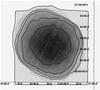 |
Fig. 1 Combined Chandra and XMM exposure map of ECDF-S area. The contours represent levels of 0.1, 1, 2, 4, 8 and 12 Ms effective Chandra ACIS-I on-axis exposure. |
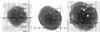 |
Fig. 2 Sensitivity of Chandra and XMM towards the detection of X-ray emission on 32′′ scales. Contours show the levels of 1.2,2,3, and 5 × 10-16 ergs s-1 cm-2 and provide the intensity scale in the image. Left: all Chandra observations. The sensitivity does not reach the deepest contour. Middle: All XMM observations. Right: Chandra plus XMM. |
For cataloguing the groups, we also include the ECDF-S data (Lehmer et al. 2005), which consist of four Chandra ACIS-I pointings, 250 ks each, defining the square shape of the exposure and sensitivity maps in Figs.1 and 2. However, a simple addition of the Chandra ECDF-S and Chandra CDF-S data results in a reduction in the quality of background subtraction in the CDF-S area, coming from the outer part of ECDF-S ACIS-I data. So for the final analysis we include the dataset with removed ECDF-S ACIS-I data in overlap with the CDF-S ACIS-I data and use the simulations of the field (Sect. 4), which reproduce the low sensitivity of the corners of ACIS-I ECDF-S mosaic.
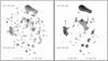 |
Fig. 3 Wavelet reconstruction of the XMM image on 32′′ − 128′′ scales without (left panel) and with (right panel) the flux removal coming from the wings of point sources. The number of apparent sources changes by a factor of 2. |
2.2. Point source subtraction
To detect and study faint extended sources, we must begin with the removal of flux produced by the point sources, following Finoguenov et al. (2009). We model the position-dependent PSF of each instrument and subtract the model from the XMM, the Chandra CDF-S and the Chandra ECDF-S mosaics separately, using the flux map of point sources derived from each mosaic. In subtracting the point sources, we operate with a flux distribution on small scales, as reconstructed using wavelets, without an attempt to catalog the sources or to use existing point source catalogs. The point source emission is resolved in Chandra, but can be confused for XMM. For XMM we remove the flux from point sources down to flux levels of 10-16 ergs s-1 cm-2 in the 0.5–2 keV band, below the a corresponding confusion limit for XMM (10-15 ergs s-1 cm-2).
For Chandra, the point source contribution to the spatial scales in excess of 16 arcsec in the central (within 3′ radius from the average aim point) detector area is negligible, while the ratio of flux on scales of 8−16 arcsec to over 16 arcsec can be approximated as a constant at large (>3′) off-axis angles Finoguenov et al. (2009). The point source subtraction procedure separates out the flux below 8 arcsec and uses the remaining flux detected within the 8−16 arcsec scale to predict the residual contamination on scales above 16 arcsec. The systematic effects associated with variation in the flux attributed to a given scale by wavelets (noisy sources have less flux detected on smaller scales) were mitigated by using the calibrated wavelet program of Vikhlinin et al. (1998) and applying three levels of flux reconstruction, with 4, 30 and 100 sigma detection thresholds and using different flux scaling for each significance level. We have verified that our flux maps for Chandra contain a contribution from all ~750 catalogued AGNs and galaxies in Xue et al. (2011). The residuals due to asymmetric PSF shapes were quantified and added as a systematical error to preclude their detection. For XMM, the selection of spatial scales used for point source flux has been explained in Finoguenov et al. (2010) and consists in absence of off-axis behaviour in the encompassed flux ratios below and above 16′′. The effect of subtracting off the contribution from point sources is extremely important for XMM, as illustrated in Fig. 3. The number of extended features is reduced by a factor of 2, and the appearance of an XMM image on 32 arcsec scales becomes similar to that of Chandra.
In Fig. 2 we show the sensitivity towards the detection of extended emission after the contamination from both background and point sources have been removed. In the 0.5−2 keV band, the Chandra data alone reach fluxes of 2 × 10-16 ergs s-1 cm-2, while XMM data alone reach 1.2 × 10⁻¹⁶ ergs s-1 cm-2. The combined dataset reaches similar depths to that of the XMM alone, but over larger area. The quoted flux corresponds to the detection cell of 0.7 arcmin2. Detailed simulations of the detection are discussed in Sect. 4.
We performed an analysis on simulated XMM maps of point sources, presented in Brunner et al. (2008) for similarly large XMM exposures in the Lockman Hole, detecting no extended emission in the simulated maps containing the detected by XMM point sources. The higher sensitivity of Chandra towards the detection of point sources allows us to make a statistical assessment of the effect of sub-threshold (for XMM) AGNs toward the detection of extended emission. Performance of XMM observations was accompanied by deepening the Chandra data within one year from each other, which makes Chandra maps suitable for XMM point source contamination analysis, limiting the effect of AGN long-term variability (Salvato et al. 2011; Paolillo et al. 2004). We have computed the variation of unresolved point source flux on the detection scales for XMM, using the Chandra image, masking out the sources detected in the XMM analysis. The constructed Chandra flux map has been further smoothed with a Gaussian of 16′′ width, approximating the effects of the XMM PSF. In the map, the uniform distribution of the faintest point sources results in nearly constant emission, which we subtract following the procedure for local cosmic background estimates for XMM, while bright sources and clustered sources make an enhancement. We find the contamination by point sources unresolved by XMM to the flux of identified extended sources is below the 5% level of the extended source’s flux. The highest peaks in the contamination map are associated with stand-alone sources near the (XMM) detection threshold, which by chance happened not to coincide with any of the detected groups and would contribute 30% to the faintest group flux. The importance of these sources is even higher in shallow surveys (Mirkazemi et al. 2015), to a degree requiring matched detection thresholds between point-like and extended sources, effectively removing faint extended sources from consideration. The importance of point source removal in XMM data is mentioned also in other cluster publications (Hilton et al. 2010; Pierre et al. 2012).
Our procedure for point source removal has been extensively tested on the real observations and is tuned for the actual XMM PSF. We have previously tested our pipeline on the simulations of the Lockman Hole (Henry et al. 2010; Brunner et al. 2008), finding no residuals. For the ECDF-S, we can extend those tests to an image a factor of 5 deeper and include the effects of sub-threshold AGNs down to fluxes of 10-17 ergs s-1 cm-2, based on the deep Chandra catalogs. In Fig. 4 we show the simulated image and the residuals detected on 32′′−128′′ scales. We have simulated point sources flux and the background for each of the XMM pointings, and followed the procedure for background and point source subtraction.
A total of 16 extended sources have been detected in the simulated 0.3 square degree mosaic image, while only point sources were used as an input. These fake extended sources correspond to large-scale distribution of unresolved sources by XMM and each source is made of a combination of typically 7 AGNs inside the source and lack of AGNs on either part of the source. We also performed a detection of simulated point sources, adding an error associated with the extra flux due to the extended sources. The number of detected fake sources has not decreased substantially (15), 8 of those are in the CDF-S area.
Finally, since the positions of the simulated sources are real, they should correspond to an actual extended source in XMM. The number of such detections in XMM mosaic is 3. This is due to the fact that most of the fake sources being close to the flux limit of 2 × 10-16 ergs s-1 cm-2, where detection is affected by the confusion on extended emission. The 3 detected fake sources have a flux of 2, 3, 5 × 10-16 ergs s-1 cm-2, with a corresponding flux error of 1.2 × 10⁻¹⁶ ergs s-1 cm-2, which agrees with the detected flux by XMM at those positions. None of these fake sources were identified as galaxy groups and entered the final catalog. However, they have contributed to a reduction in the identification rate by 6%. In Fig. 5 we overlay the contours of detected extended emission over the simulated point source contamination image.
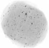 |
Fig. 4 Simulated XMM mosaic image of point source and background emission in the ECDF-S. |
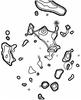 |
Fig. 5 Simulated residuals after the point source removal and background subtraction. Contours show the detected X-ray emission. We identify three detected false sources (highlighted by dashed circles). None of these sources were identified as a galaxy group. |
In Fig. 6 we show the signal-to-noise ratio (S/N) obtained for the final joint dataset (excluding ECDF-S Chandra data) after subtracting the background and detected point sources. The white part of the image corresponds to zero or negative signal. The grey and black parts of the image correspond to an area with significant flux, which occupies a substantial (20%) part of the image. There are three large sources: one in the east, associated with a nearby group; one in the north, associated with a nearby cluster having a peak outside the area of ECDF-S, but seen clearly in the ACIS-S chip that was on during the observation; the third source, which is near the center, is due to confusion of several groups with overlapping virial radii. We will return to the modelling of the image in Sect. 4.1.
2.3. Source extraction
The sensitivity of the source detection depends critically on the background per resolution element. The level of the background per unit area is comparable between Chandra and XMM. On small scales, the XMM PSF leads to large corrections for the encompassed flux of the source, which reduces the effective XMM sensitivity towards point sources. On scales selected for the analysis in this paper, the PSF does not affect the source flux, but there is an induced background due to a distribution of AGN counts by larger PSF of XMM. These differences support a consideration of separate Chandra and XMM searches for the extended sources, in addition to a joint search.
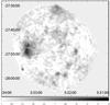 |
Fig. 6 Signal-to-noise of the XMM data after point source removal and smoothing with a 16′′ Gaussian kernel. The color bar shows the correspondence between the color and the significance of the emission, starting with white for −1σ. |
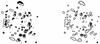 |
Fig. 7 Left: XMM detection of extended emission on a 32 arcsec scale. Right: Chandra detection of extended emission on a 32 arcsec scale. Contours, which are the same in both panels, show the extended emission detected in the combined Chandra and XMM images on the 32 and 64 arcsec scales. Full ECDF-S field of 0.3 sq.degrees is shown. |
Sources found in deep X-ray surveys are primarily AGNs and distant galaxies (Brandt & Hasinger 2005). Groups and clusters of galaxies only account for 10% of the cosmic flux (e.g. Finoguenov et al. 2007). Their emission on arcminute scales requires different detection methods versus compact sources. Most techniques to date refer to detection of galaxy groups and clusters as extended sources.
The term extended emission is however loosely defined. To some extent any astrophysical emission results from objects that are not singular and so it is only a question of how extended the emission is. Emission on scales of a few arcseconds in the survey data appears to stem from the cores of the groups, X-ray jets, galaxy mergers and even individual galaxies.
An important characteristic of group X-ray emission is a correlation between its intensity and angular extent: the emission typically covers a sizable fraction of the R500 radius that can be derived based on the observed flux and a known source redshift. Groups of galaxies that are sufficiently bright to be detected in X-rays, exhibit emission on arcminute scales even at the highest redshifts accessible to the deepest surveys like the ECDF-S. As the detection is background limited, and given the shape of the surface brightness profile of galaxy groups, the emission on smaller scales is more easily detectable. The adoption of spatial scales of 32′′ is therefore a trade-off between S/N on one hand and both telescope characteristics and source identification, on the other. The depths of the ECDF-S preclude using large spatial scales, as due to the high number of extended sources the emission is confused on the arcminute scales.
In Fig. 7 we compare the final detection map with the individual maps obtained by Chandra and XMM. The most significant sources appear in both maps. For the final detection, we combined the residual maps of the Chandra ECDF-S, CDF-S and XMM ECDF-S. The practical issue of the combining maps with different pixel sizes is handled using the TERAPIX SWARP software. We co-add the residual counts without any weight, co-add the exposure maps re-normalised to differences in the effective areas of the instruments and add the error maps in quadrature. The sensitivities of Chandra and XMM towards the X-ray emission in the 0.5–2 keV band also depend on the spectrum of the group emission, while in adding the data we can only assume a typical ratio of the sensitivities. Large differences in the ratio of sensitivities occur only if the emission is primarily at energies below 0.7 keV, where also the differences between pn and MOS are large. In Fig. 8 we compare the XMM and Chandra fluxes for the sample. We use the effective exposure units, in which the count-rate of XMM and Chandra are similar. We view Fig. 8 as a characterisation of the scatter introduced by our attempt to merge XMM and Chandra raw counts, which is of the order of 0.2 dex. A few bright objects are located at the outskirts of the observations and also occupy a large area, leading to instrument-specific differences in the background prediction.
3. Identification of galaxy groups
All sources in our catalog are X-ray selected, using the emission from outskirts of the groups, typically exceeding 100 kpc scales (with any exception from this criteria duly noted), uniquely identifying galaxy groups even at low luminosities. X-ray data alone are not sufficient for source identification and thus our effective survey sensitivity is a combination of both X-ray and optical/NIR sensitivities. For example, Bielby et al. (2010) demonstrated that deep NIR data are essential to identify distant groups and clusters of galaxies. In this work, we combine the ultra-deep X-ray observations of the ECDF-S with the exquisite optical-nearIR photometric and spectroscopic data available in the field.
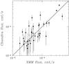 |
Fig. 8 Flux comparison between Chandra and XMM within the area covered by the 4 Ms Chandra CDF-S. The solid line shows the 1:1 correspondence. 38 extended sources with significant flux measurement in both Chandra and XMM data are shown. The errors on XMM fluxes are similar to the plotted Chandra errors and are omitted from the plot for clarity. |
We run our red sequence finder (Finoguenov et al. 2010; Bielby et al. 2010) around the central portions of all the X-ray group candidates. We base our red sequence search on the Penn State photometric redshift catalog described in Rafferty et al. (2011). We first extract galaxies around a redshift of interest by applying | zphot − z | < 0.1. We then count galaxies around the model red sequence constructed with the Bruzual & Charlot (2003) model (see Lidman et al. 2008 for details). When counting, we use a Gaussian weight in the form of ![Mathematical equation: \begin{eqnarray*} &&\sum_i \exp\left [ -\left (\frac{{\rm color}_{ i, {\rm obs}}-{\rm color}_{\rm model}(z)}{\sigma_{i,{\rm obs}}}\right )^2\right ]\nonumber\\ && \times\exp \left [-\left ( \frac{{\rm mag}_{i,{\rm obs}}-{\rm mag}^*_{\rm model}(z)}{\sigma_{\rm mag}}\right) ^2\right ]\times \exp \left( -\left(\frac{r_i}{\sigma_{\rm r}}\right)^2\right) , \end{eqnarray*}](/articles/aa/full_html/2015/04/aa23053-13/aa23053-13-eq31.png) where colori,obs and magi,obs are the color and the magnitude of the ith observed galaxy, σi,obs is the observed color error in colori,obs, colormodel(z) is the model red sequence color at the magnitude of the observed galaxy,
where colori,obs and magi,obs are the color and the magnitude of the ith observed galaxy, σi,obs is the observed color error in colori,obs, colormodel(z) is the model red sequence color at the magnitude of the observed galaxy,  is the characteristic magnitude based on the model, which is tuned to reproduce the observed characteristic magnitudes, σmag is the smoothing parameter and is set to 2.0 mag, ri is the distance from the X-ray center and σr is another smoothing parameter with 0.5 Mpc. In our earlier work (Finoguenov et al. 2010), we adopted σr = 1 Mpc, but here we apply a smaller window of 0.5 Mpc because we search for both smaller and more abundant (we therefore need to reduce the chance association) systems. The significance of the red sequence around an X-ray source is computed with respect to the mean and variance of the number of red galaxies measured at random positions in the same field.
Bands employed in the red-sequence technique.
Since different colors are sensitive to red galaxies at different redshifts, we adopt the combination of colors and magnitudes summarised in Table 1. We use the publicly available MUSYC photometry in the ECDF-S area (Gawiser et al. 2006), which is slightly smaller than the full X-ray coverage. In the GOODS area, we use the deeper public catalog from the MUSIC survey (Grazian et al. 2006; Santini et al. 2009). Our experience shows that we need to go down to ~ M∗ + 1 to securely identify a red sequence. High redshift systems lack faint red galaxies, but the red sequence is often seen down to that magnitude (e.g., Tanaka et al. 2007). The MUSYC data for ECDFS is not deep enough to identify z ≳ 1.5, and thus high-z identifications are not yet complete at present. The MUSIC data is deep enough to see systems at z = 2 and beyond. In fact, we have identified two z ~ 1.6 groups as discussed below.
One may worry that a red sequence finder introduces a bias; it may miss groups dominated by blue galaxies. But, we note that a red sequence finder misses only groups in which the red fraction is significantly smaller than the field. Suppose the red fraction in a group is the same as the field, a group is an over-density of galaxies by definition and thus there is a larger number of red galaxies within a small volume, which will then be detected by a red sequence finder. It is an interesting question if groups with a lower red fraction than the field exist at high redshifts. They may, but recent observations of z ~ 2 systems, especially those in the process of forming, show red sequence (e.g., Tanaka et al. 2013b). This might indicate that red sequence is a ubiquitous feature of groups and clusters since an early epoch.
In the identification process, we have made an extensive use of spectroscopic redshifts available in the field. The X-ray data used in this work covers a 0.3 square degree area, which is larger than the 0.1 square degree area of GOODS-S, where extensive public ESO spectroscopic surveys have been carried out (e.g. Balestra et al. 2010). Two spectroscopic campaigns have been used to remedy this situation: ECDF-S follow-up through devoted ESO and Keck efforts (Silverman et al. 2010), and since 2009, the follow-up of groups has been carried out by the ACES project (Cooper et al. 2012), which is a large program on the Magellan telescope. We have complied a spectroscopic catalog with a high sampling rate (60% down to i = 22 AB mag) from these efforts. We replace red sequence redshifts with spectroscopic redshifts where available. Large amount of spectroscopy available in the field, enables a search for the spectroscopic galaxy groups, with most massive ones having a good correspondence to the location of X-ray emission (Dehghan & Johnston-Hollitt 2014).
4. Modelling of the X-ray source detection procedure
In this section we provide the validation of the X-ray detection method. Readers not interested in the technical details of the X-ray detections may skip to Sect. 5.
Our method of detection of extended sources differs from other X-ray surveys. Most X-ray cluster surveys aim to fit a symmetrical beta model with a fixed beta to a list of extended source candidates, resulting in the determination of the cluster core radius. This modelling of the surface brightness profile is later used to infer the total flux of the cluster within some radii (Pacaud et al. 2007; Lloyd-Davies et al. 2011). If we revisit the origin of the method, the reasoning for using it comes primarily from low-redshifts, where the core is well resolved, while outskirts of the cluster are not observed. The high reliance of X-ray surveys on the core properties of clusters has been argued by a number of studies as a weakness, as it introduces a large scatter in cluster selection, favouring the detection of clusters with strong cool cores. On the other hand, it has been argued (Vikhlinin et al. 2009) that cluster outskirts exhibit a much smaller scatter with total mass, as witnessed in the low-scatter of core-excised LX (Maughan 2007). The reported low-scatter measurements were obtained using a simple aperture flux. It therefore seems logical to pursue a method of cluster detection, which would only be sensitive to flux coming from outskirts. In addition, resolving the core of a high-z group is only possible with the on-axis PSF of Chandra, while for XMM resolving cores below 10′′ is both incomplete (Lloyd-Davies et al. 2011) and is subject to contamination from point sources (Pacaud et al. 2007). For redshifts above 0.5, detecting the outskirts beyond half of the R500 value is typical.
The low scatter of core-excised LX suggests that the cluster surface brightness profile can be modelled as a sum of two profiles, one describing the core and the other describing the outskirts with the ratio of core to R500 radii and values of beta similar to that of merging clusters. While this is yet to be verified, it implies a low-scatter scaling between the detected flux in the fixed aperture and the core-excised LX in the region enclosing the flux calculation. Deviations from this assumption would violate the published low scatter of gas mass presented for a wide range of overdensities, from 2500 to 500 (Allen et al. 2008; Vikhlinin et al. 2009; Okabe et al. 2010), which brackets the overdensities important for this work. Given these considerations, we assume that we can restore the core-excised flux of the group based on the detection of group outskirts.
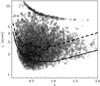 |
Fig. 9 Distribution of core radii of the detected simulated extended sources. The shades show the detected sources in the “Confusion” run, with shades of grey illustrating the overlap of sources. The dashed and solid lines show the location of 90% and 50% detection completeness level. The core radii are uniquely determined by the mass and redshift of the halo, using the tabulations of Finoguenov et al. (2007). |
In order to model the X-ray detection of groups in ECDF-S, we explore different aspects of the group detection. Using the sensitivity map, presented in Fig. 2, we calculate the limiting group mass that can be detected for each area of equal sensitivity, using a grid of redshifts and adopted scaling relations with total mass. For each limiting mass, redshift, and volume, corresponding to equal sensitivity areas and steps of the redshift grid, we generate simulated groups with masses according to the mass function, defined by LCDM with the Planck cosmological parameters (Planck Collaboration XXVI 2014). In adopting the set of parameters we select the Planck CMB only constraints (no BAO), which are also close to WMAP9. The values of the cosmological parameters assumed are Ωm = 1 − ΩΛ = 0.30, σ8 = 0.81, h = 0.7.
With about 100 groups expected from the cosmology, we would not be able to sample well all the parameter space important for detection and so the expected numbers were boosted by a factor of 100, constrained by the time required to perform the simulations. The positions of the groups were randomised within the sensitivity area and the redshifts were randomised within the resolution of the redshift grid. In simulating the halos with masses in excess of 1014M⊙, we do not follow the shape of the mass function in detail, but calculate the integral of the mass function above 1014M⊙ and upon boosting and randomising the total number of simulated systems, and we assign the 1014M⊙ mass to all such sources. This creates an upper boundary in the point distribution visible in Figs. 9–13.
As a second step, we run direct simulations of the group detection. For each group, we used the total mass to establish R500 and the tabulations of Finoguenov et al. (2007) to predict the parameters of the beta model. The limiting flux of the detection is translated to the limiting value of beta and core radii. Figures 9 and 10 illustrate the values of core radii and beta as a function of redshift for detected sources. We show the curves of incompleteness, calculated for the CDFS area, showing where we start loosing sources, which is determined by the flux on the detection scales. Most high-redshift groups have an expected extent of their X-ray emission (R500) comparable to the detection scale used, while the values of their core radii can only be resolved by Chandra. As a result of the point source removal applied, the cores of the simulated groups are removed as well and the detection is only sensitive to the flux at the group outskirts, while the extent of the simulated detection approaches R500. At z< 0.3 the core of the group becomes detectable, and variations in the inner group surface brightness become important. The simulations generate the group profile, and projects it on the exposure map. This provides a model to further pixel-wise randomisation of a number of photons detected and the model for errors which we add to the survey noise map.
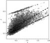 |
Fig. 10 Distribution of the beta parameter of the detected simulated extended sources. The shades show the detected sources in the “Confusion” run, with shades of grey illustrating the overlap of sources. The dashed and solid lines show the location of 90% and 50% detection completeness level. The value of beta is uniquely determined by the mass and redshift of the halo, using the tabulations of Finoguenov et al. (2007). |
Summary of simulations of X-ray group detection in ECDF-S.
Table 2 summarises the results of source detection simulations for two choices of scaling relations, the COSMOS one and adopting a 30% higher mass for given total Lx, to mimic the effect of our calibration uncertainties. The later are termed as “Scaling” runs. The basic run is termed “Sensitivity only”. We consider the additional effects of confusion and confusion+PSF. We cull our input group list for simulation near detection boundary, based on the experience with sampling the parameter space.
To simulate the effect of confusion, we reran the simulations, adding simulated groups to the actual ECDF-S image. We require the peak of the emission to be within 16′′ of the original center. We remove the area within 16′′ from the peaks on the X-ray image, as those would always be detected. These peaks occupy 5% of the total area. As seen in Table 2 (“confusion” run), accounting for confusion leads to further reduction in the total number of sources, however due to the statistical nature of the detections and enhanced detection of the emission at places near the existing sources produces a small number (2%) of detections in this run, which were not obtained in the previous one.
To simulate the differences in the source detection between Chandra and XMM, we performed another round of simulations with confusion, in which we convolved the source profile with the XMM PSF and in the detection procedure we introduce a step of flux removal from large scales, based on the detection on small scales. We find (Table 2, “Confusion+PSF” run) that the main result is a 2% increase in the detection rate. Thus, we conclude that XMM PSF only marginally inhibits the detection of groups in our algorithm, compared to running it on the Chandra data. The origin of the effect is due to tuning of the flux removal for the point sources, leaving in a fraction of the flux from the group cores scattered by XMM PSF to outskirts of the groups. In the “Scaling” runs, we only considered the effects of change in the scaling and confusion (Table 2).
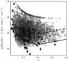 |
Fig. 11 Flux-redshift plane of the ECDF-S sample (filled circles with error bars). The grey shades show the distribution of the parameters of the detected groups in simulations, with Planck cosmological parameters (Planck Collaboration XXVI 2014) and the scaling relations of Leauthaud et al. (2010) used. Due to the limited spatial scales used, at low redshifts the effective sensitivity towards the total flux is lower. The upper boundary on the flux distribution shows the combination of the ECDF-S survey volume and cosmology. The dashed and solid lines show the location of 90% and 50% detection completeness level. |
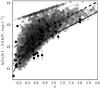 |
Fig. 12 Luminosity-redshift sampling in the ECDF-S. Grey shadowing indicate the density of detected groups in simulations, with Planck cosmological parameters (Planck Collaboration XXVI 2014) and the scaling relations of Leauthaud et al. (2010) used. Solid circles show the parameters of ECDF-S groups. The dashed and solid lines show the location of 90% and 50% detection completeness level. |
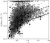 |
Fig. 13 Mass-redshift sampling in the ECDF-S. Definition of mass is done with respect to the mean density and is scaled by the Hubble constant. Grey shadowing indicate the density of detected groups in simulations, with Planck cosmological parameters (Planck Collaboration XXVI 2014) and the scaling relations of Leauthaud et al. (2010) used. Solid circles show the parameters of ECDF-S groups. The dashed and solid lines show the location of 90% and 50% detection completeness level. |
We can compare the results of the simulations also to the combined XMM+Chandra catalog. We use the results of the “Confusion” run. We illustrate the detections in Fig. 11. The simulations allow us to show the expected completeness of X-ray group detection as a function of luminosity or a group mass, which we illustrate in Figs. 12 and 13. We show the completeness curves calculated for the CDFS area in Figs. 9−13. In Table 3 we summarise for the three representative flux levels the properties of the survey in terms of contamination and present the estimates of the completeness at z = 0.6, with account for the effect of confusion. In Fig. 11 we also see a gradual loss of sensitivity towards the group detection with increasing redshift at z > 0.6 caused by the reduction in the angular size of R500.
Contamination and completeness of X-ray group detection in ECDF-S.
Outside the radius of three core radii, for a given slope of the surface brightness profile, the scaling of the emission from one spatial bin to another does not depend on the actual value of the core radius, as can be shown analytically. Since we consider the variation of the central luminosity of the X-ray group as a source of scatter, ignoring this variation shall be understood as the low-scatter part of LX, just-like the core-excised LX. The absolute value of the LX can deviate even from the average LX for groups of a given flux and redshift. For the purpose of inferring the group mass, this requires calibration, for which we use external methods, such as clustering and weak lensing. Thus, even if the actual group parameters would systematically deviate from the assumed ones and exhibit the scatter, we can still rely on our method of assigning the total mass. The actual scaling relation will however be method (and thus instrument) dependent. In our modelling, we go from the cosmology to the mass function, and then to the expected LX given the calibrations suitable for our parametrisation of the surface brightness profile and later evaluate the detection. Should we change the surface brightness profile parametrisation, the scaling relations would have to be changed to compensate for the change in the flux in the detection cell. The actual variation of the flux on large scales for a given mass is expected to be as small as the reported behaviour of core-excised LX, which is 7% for clusters, according to Maughan (2007), which is negligible, compared to the statistical scatter for the simulated (and used) 4σ detection limit.
Our modelling is performed under an assumption of no evolution of the fraction of surface brightness associated with 0.1R500. Existing statements in the literature, indicate that if any, the cool core contribution to the total flux is reduced. Thus we believe that our assumptions are conservative. For comparison with literature, we note that the importance of the emission inside the core radius is much higher for steep beta values, like 0.6, which is typically assumed for and is a characteristic of massive clusters.
4.1. Understanding the effect of group outskirts in explaining the X-ray image
The high spatial density of sources, identified in the ECDF-S exposures, should result in largely overlapping emission on large scales. To test this effect, we use the identified systems to model the X-ray image on large spatial scales. We assumed a beta model for each of the groups with core radii equal to 10% of the virial radius and a slope β = 0.6. High β = 0.6 values assumed, can be viewed as conservative for estimating the source confusion on large scales, as the surface bright profile for each source drops fast. The normalisation is chosen to match the aperture flux of the source. The simulated exposure approximately matches the achieved sensitivity. A flat exposure map and 5′′ PSF are adopted, using the SIXTE (Schmid et al. 2010) Athena WFI set-up. These differences are not important for making our point. To compare the simulated image with the observed one, we applied the same wavelet reconstruction procedure and in Fig. 14 compare the detected emission on 0.5−2 arcmin scales. The revealed similarity in the image is quite striking. The details of the arcminute-scale variation in the X-ray emission are well reproduced. This emission caused problems for estimating the sky background, in the northern and eastern part of the survey, leading us to use the central vs. western part of the survey for in-field estimates of instrumental vs. sky background components. The complex bright structures on 2′ scales in the ECDF-S are reproduced as an effect of confusion on large scales. And even the complex appearance of the sources on arcminute scales seems to be sufficiently modelled as the confusion of several sources (e.g. the “Fudge” source is a combination of four galaxy groups).
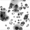 |
Fig. 14 Wavelet reconstruction of the simulated image of extended emission in the ECDF-S area on scales of 0.5−2 arcmin. The contours of the observed X-ray emission on matched spatial scales are overlaid in black. Contours not aligned with simulated X-ray emission correspond to unidentified sources. The contours do not show the largest scales of the emission, but similarity between the model image and the S/N image in Fig. 6 is clear. |
5. Galaxy groups in the ECDF-S field
5.1. The Group catalog
In this section we describe our catalog of 46 X-ray galaxy groups detected in the ECDF-S field as well as estimates for the 5 components of the Kurk structure (Kurk et al. 2009). In the catalog (Table 4) we provide the source identification number (Col. 1), IAU name (Col. 2), RA and Dec of the X-ray source in Equinox J2000.0 (3−4), and redshift (5). The cluster flux in the 0.5−2 keV band is listed in Col. (6) with the corresponding 1 sigma errors. The flux has units of 10-16 ergs cm-2 s-1 and is extrapolated to an iteratively determined R500 (see Finoguenov et al. 2007, for details). The aperture determining the flux has been defined by the shape of the emission on 32′′ scales, unless it has been manually redefined to avoid contamination from other extended sources (cases where this is not possible have flag = 4). The total net XMM+Chandra counts in the flux extraction region are given in (7). The rest-frame luminosity in the 0.1−2.4 keV band in units of 1042 ergs s-1 is given in (8), where the K-correction assumes the temperature from the scaling relations adopted in Finoguenov et al. (2007). The choice of the energy band is driven by the available calibrations of the Lx − M relation (Leauthaud et al. 2010), yielding (Col. 9) an estimated total mass, M200, defined with respect to the critical density, with only the statistical errors quoted. Systematic errors due to scatter in the scaling relations are ~20% (Allevato et al. 2012) and the uncertainty on the calibration is 30%, as discussed in Sects. 6 and 7. The corresponding R200 in arcminutes is given in Col. (10). Column (11) lists the source flag and the number of spectroscopic member galaxies inside R200, used to evaluate the mean spectroscopic redshift, is given in Col. (12). In Col. (13) we provide the predicted galaxy velocity dispersion based on the Carlberg et al. (1997) virial relation using our total mass estimates. A comparison between these and actual measured values of Vdisp is presented in Erfanianfar et al. (2014). The errors provided on the derived properties are only statistical and do not include the intrinsic scatter in the LX − M relation and the systematics associated with the extrapolation of the scaling relations to lower luminosities at similar redshifts. In Sect. 6 we successfully verify these masses by means of a clustering analysis to a precision below the 0.2 dex uncertainty of individual mass estimates due to the scatter in M − LX relation. In Sect. 7 we also successfully verify the mass calibration by means of stacked weak lensing analysis.
While a number of groups we report on were previously discovered by Chandra, their emission has only been probed out to much smaller radii, and so it was much more uncertain as a characterisation of the group properties. This poses a trade-off for optimising future telescope performance, as detection benefits from high angular resolution, while the characterisation benefits from low background and collecting area.
There is an issue related to the definition of the extended source flux, corresponding to quotation of the source flux. In Giacconi et al. (2002) and Bauer et al. (2004) the detected flux is quoted, while in Finoguenov et al. (2007, 2010) the full flux of the source is quoted. These can be different by a factor of a few. Using the large spatial scales, one reduces the amount of extrapolation on the flux and therefore removes a large separation between the observed and referred flux, which is subject to model assumptions (Connelly et al. 2012).
In Finoguenov et al. (2007, 2010), Bielby et al. (2010) we introduced a system of flagging the source identification. The objects with flag = 1 are of best quality, with centroids derived from the X-ray emission and spectroscopic confirmation of the redshift; flag = 2 objects have large uncertainties in the X-ray center (low statistics or source confusion) with their centroids and flux extraction apertures positioned on the associated galaxy concentration with spectroscopic confirmation; objects with flag = 3 still require spectroscopic confirmation; objects with flag = 4 have more than one counterpart along the line of sight; objects with flag = 5 have doubtful identifications and are only used to access systematic errors in the statistical analysis associated with source identification.
Using a catalog of Miller et al. (2013) we find a number of complex radio sources inside the X-ray galaxy groups, the correspondent group ids are: 3, 12, 19 (contains a Wide Angular Tail source), 26, 43, 52, 57. All these sources do not have a two-dimensional match of the shape of their X-ray emission with the radio. In all cases, but group 43, we can also rule out a substantial (>10%) contribution of the IC emission associated with radio source to the X-ray flux. For group 43 this contribution can be up to 50%, estimated using the part of the source flux in the area overlapping with the radio emission. We note that the associated with group 43 radio galaxy is the strongest FRII source in CDFS. Other studies typically find one IC X-ray source per square degree (Jelić et al. 2012), so the statistics of CDFS is consistent with that.
5.2. Statistical properties of the groups
In Fig. 11 we plot the sample in the flux-redshift plane. The confusion of sources and our approach to reduce it using 32′′ spatial scales for the flux extraction, results in large flux corrections at low-z. The correction approaches unity (thus no correction at all) for z > 0.5 sources with a high significance of the detection. This also introduces a redshift dependence to the flux limit, with a limiting flux of 10-15 ergs s-1 cm-2 at z = 0.05 levelling off at 1.5 × 10⁻¹⁶ ergs s-1 cm-2 at the redshifts exceeding 0.5. However, to account for this effect is straight-forward. Our experience shows that different science goals require different subsamples, a mass-limited sample, for example, would be selected differently. Also, some definition of galaxy groups would make a cut on X-ray luminosity, removing the need for an equal flux. For most of our own work, the high-z galaxy groups are the ones that we are most interested in (Ziparo et al. 2013, 2014).
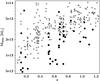 |
Fig. 15 Comparison of the mass-redshift sampling of the ECDF-S (filled black circles) and COSMOS (filled grey circles) X-ray group samples. Definition of mass with with respect to the critical density. The ECDF-S groups extend to much lower masses, while occupying a similar redshift range. An improvement in the mass sensitivity of the survey scales as exposure to the power of 3.3, so 30 times deeper data in ECDF-S results in a 3 times better mass limit. |
The X-ray detected groups span a large range of X-ray luminosities (1041 − 1043 ergs s-1). The total masses of the X-ray groups are derived by applying the empirical LX–M200 relation determined for the COSMOS groups in Leauthaud et al. (2010) via the weak lensing analysis. Figure 15 shows the derived mass range and compares it to the calibrated range in the COSMOS survey (George et al. 2011). The ECDF-S groups occupy a unique mass-redshift space, which influence our understanding of galaxy evolution in the group environment. This is explored in the dedicated follow-up papers (Popesso et al. 2012; Ziparo et al. 2013, 2014; Erfanianfar et al. 2014). The resulting ECDF-S sample of X-ray detected groups ranges between 5 × 10¹² and 5 × 10¹³M⊙. For the first time, the derived masses cross the 1013M⊙ mass range, much below the typical X-ray group mass of 5 × 10¹³.
5.3. Consistency with cosmology
In Fig. 13 we compare the masses and redshifts of the detected groups with the density of groups, expected from the Planck cosmology (Planck Collaboration XXVI 2014) and the scaling relations of Leauthaud et al. (2010). One can see that the two bright low-z groups are unusual for the size of the field, while there is a lack of structure at 0.2 < z < 0.5.
Most previous studies, which reported the counts from extended sources in deep surveys (Giacconi et al. 2002; Bauer et al. 2004; Finoguenov et al. 2007, 2010) primarily report the emission identified with galaxy groups. Also the modelling of log N − log S of extended sources assumes that it stems from groups and clusters of galaxies.
In Fig. 17 we show the log (N>S) − log (S) of X-ray groups in ECDF-S. The data are consistent with the prediction of no evolution in the XLF from Rosati et al. (2002) down to 10-16 ergs s-1 cm-2 fluxes, where the predicted number of groups is 500 groups per square degrees and the measured values are bounded by the 300−700 range. A power law approximation to the log N − log S gives an index of −0.85 (or 1.85, conventionally used for AGN differential log N − log S). We have not corrected for the faint low-z groups that cannot be detected in our survey, but this correction is small due to the low volume at low-z.
We find that the observed counts are consistent with number counts predicted for a flat ΛCDM Planck cosmology (Planck Collaboration XXVI 2014) with Ωm = 0.3 and h = 0.7 and σ8 = 0.81, when the results of the simulations of the source detection in ECDF-S and the scaling relations of Leauthaud et al (2010) are combined. We note that the differences in the cosmological parameters affect only mildly the derivation of the scaling relations. As explored in Taylor et al. (2012), the sensitivity of lensing geometry for COSMOS group experiment to ΩΛ is 0.15 at 68% confidence level, while the differences to Planck cosmology are much smaller, 0.04.
The predicted number of sources in the Planck cosmology (Planck Collaboration XXVI 2014) and the scaling relations of Leauthaud et al. (2010), combined with the presented detailed simulations of the source detection in ECDF-S is marginally inconsistent with the data. Introducing the 30% deviations in the scaling relations, allowed by our calibrations, is required to reproduce the best fit log N − log S.
Figure 16 compares the X-ray luminosity function in ECDF-S with that of COSMOS (Finoguenov et al. 2007) and the local measurements based on RASS (Böhringer et al. 2001). In computing the X-ray luminosity function (XLF), we limit the sample to z < 1.2, where our spectroscopic follow-up is complete, and we can account for our redshift cut through the volume calculation. We illustrate the sample variance within the ECDF-S by using the full and partial areas of the survey, which also probes the importance of the completeness correction. We find the statistical and systematic errors on the XLF to be similar. We correct for the detection completeness using the simulations. This introduces a different limiting redshift, as a function of luminosity at which the detection is complete. While in the calculation of XLF this is simply the effective volume, there is a difference in the effective maximum redshift probed by the data as a function of the luminosity, which limits the statement about the XLF redshift dependence. At luminosities near 1043 ergs s-1, no evolution of XLF between z < 0.6 and 0.6 < z < 1.2 has been previously shown by Finoguenov et al. (2007) using COSMOS data. ECDF-S both extends the measurement of XLF down to unprecedented luminosities of 1041 ergs s-1 sampled at z < 0.2 and samples groups with LX of 3 × 1042 ergs s-1 to a redshift of 1.2. So in agreement with the COSMOS data, which sampled those systems to a redshift of 0.6, our current work extends the claim of no evolution in XLF down to luminosities of 3 × 1042 ergs s-1. We note that this is not a trivial addition to the previous COSMOS result for 1043 ergs s-1, given that feedback processes are expected to play an important role at low-luminosity groups, which might cause differences in the evolution of XLF as a function of luminosity. While all dataset probe groups at 1042 ergs s-1 luminosity, the maximum redshift for a detecting such systems changes from 0.02 for the RASS (and the differences between North and South can be interpretted as sample variance), to 0.3 for COSMOS to 0.6 for the ECDF-S. No evolution at low LX does not contradict to the results on XLF evolution at Lx > 5 × 1044 ergs s-1 (Koens et al. 2013) driven by the massive cluster growth.
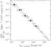 |
Fig. 16 X-ray luminosity function of ECDF-S groups. Black dots show the measurement using the full field, while black crosses show the measurements excluding the central region where there is a low spatial density of groups. Gray crosses show the results from the COSMOS field. Dashed and dotted curves show the local XLF in the Northern and Southern Hemisphere, revealing an effect of sample variance, caused by small volumes probed by RASS at low group luminosities. |
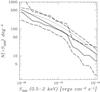 |
Fig. 17 log (N>S) − log (S) of X-ray groups. The grey curves show ECDF-S data and the 1σ envelope shown as dashed curves. The solid black curve shows the prediction of a non-evolving X-ray luminosity function from Rosati et al. (2002). The long-dashed line shows the simulated detected counts using Planck cosmology (Planck Collaboration XXVI 2014) and the Leauthaud et al. (2010) scaling relation. The dotted line, illustrates the effect on changing the normalisation of scaling relations by increasing the associated mass by 30%, allowed by our calibration at faint fluxes (below 10-15 ergs s-1 cm-2). |
The conclusion on the absence of strong XLF evolution at the luminosities below 1043 ergs s-1 is in agreement with the log N − log S modelling, which is best fit by the non-evolving XLF. In the probed range of X-ray luminosities, no detectable evolution in the XLF is expected from a combination of cosmology (reducing the number of groups of a given mass) and evolution of scaling relations (increasing the X-ray luminosity of each group for a given mass) adopted in our work (Finoguenov et al. 2010).
Figure 18 shows the dn/dz/dΩ distribution of the ECDF-S groups. The grey curve shows the cosmological prediction with parameters fixed to the Planck13 cosmology and the scaling relations of Leauthaud et al. (2010) (solid curve) and a 30% change in the normalisation of the scaling relations allowed by our calibration (dashed curve). We conclude that sample variance, discussed above is caused by the lack of structure at 0.2 < z < 0.5 and marginally at 1.2 < z < 1.5, while at other redshifts the ECDF-S can be considered as a representative field. We further note that the modelling of dn/dz/dΩ is sensitive to the detection of systems at the detection limit. More work on understanding the variety of shapes of the intragroup X-ray emission is needed in order to derive conclusions on the cosmological parameters implied by the survey. As an example, many of the groups reported here have been previously detected but assigned a much smaller flux. On the other hand, some of the new detections have fluxes above the formal limits of previous work, illustrating how the variety of shape results in the source detectability. While we attempt to account for this effect, our model parameters are fixed to the local measurements (Finoguenov et al. 2007), which might not be representative for the high-z groups. The problem with the flux correction is most important for systems at the detection limit, as only part of the source is detected. The low statistics prevent us from evaluating dn/dz/dΩ for the high-flux subsample.
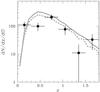 |
Fig. 18 dn/ dz/ dΩ [deg-2] distribution of the ECDF-S groups (black crosses). The prediction from the detailed detection simulation and Planck cosmology (Planck Collaboration XXVI 2014) is shown as solid grey curve and the effect of 30% change in the scaling relations is shown by the dashed grey curve. |
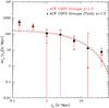 |
Fig. 19 Projected autocorrelation function of X-ray galaxy groups in the ECDF-S. The red points show the results for all the groups and the black points again for groups but excluding the central area from both real and random catalogs. As we discuss in the text, we do not see any significant change in the results, after introducing the method for correcting the first order effects from cosmic variance. The dotted lines show the two-halo terms |
6. Auto-correlation function of groups
We can use the two-point correlation function to measure the spatial clustering of galaxy groups and to estimate their total mass. With 40 spectroscopically identified groups we just have enough systems to constrain these statistics. We use the same random catalog that has been used throughout the paper and apply the Landy-Szalay estimator (Landy & Szalay 1993). To separate the effects of redshift distortions we measure the spatial correlation function in projected separations between groups in the direction perpendicular (rp) and parallel (π) to the line-of-sight. We then integrate over the velocity (π) component of the correlation function. Figure 19 shows the projected correlation function, wp(rp) (Davis & Peebles 1983), which removes the effect of infall on the clustering signal. In the halo model approach the amplitude of the group clustering signal at large scale (two-halo term) is related to the typical mass of the galaxy groups through the bias factor. In detail,  (1)In performing this analysis, we merge the groups within r200 of each other (Allevato et al. 2012), which removes the one halo term in the correlation function. As shown in Fig. 19, at projected separations exceeding 1 Mpc h-1, the shape of the galaxy groups correlation function is well-fit by the two-halo term. The measurement of an excess clustering signal at 0.2 Mpc h-1 indicates that non-linear gravitational collapse is nevertheless affecting the signal, so extension of the comparison between the prediction for the linear growth of the two halo term to rp < 1 Mpc h-1 is not supported by the data.
In modelling we compare the measured amplitude of the two halo term with the prediction of linear biasing using the mass of each group that contributed to pair statistics and weighted with the large-scale structure (LSS) growth function. In detail, for each galaxy group ith at redshift zi, we estimate the bias factor corresponding to a DM halo mass M200 (h-1 Mpc):  (2)where b(M200,zi) is evaluated following the bias-mass relation described in Sheth et al. (2001). The linear regime of the structure formation is verified only at large scales, which is further confirmed by our data in Fig. 19, so we estimated the average bias of the sample, including only the pairs which contribute to the clustering signal at rp = 1 − 40 Mpc h-1. As described in Allevato et al. (2011), we define a weighted bias factor of the sample as:
  (3)where bibj (each defined by Eq. (2)) is the bias factor of the pair i − j and Npair is the total number of pairs in the range rp = 1 − 40 Mpc h-1. The D factor is defined by D1(z) /D1(z = 0), where D1(z) is the growth function (see Eq. (10) in Eisenstein & Hu 1999, and references therein) and takes into account that the amplitude of the DM two-halo term decreases with increasing redshift. We verified that the bias factor estimated using the correlation function of galaxy groups (Eq. (1)) is consistent with the weighted bias factor (bpredicted).
For all (40) groups with flag ≤ 3 and z < 1.3, we find a best fit bias bobs = 2.28 ± 0.25, estimated using a  minimisation technique with 1 free parameter, where
  , Δ is a vector composed of
  and Mcov is the covariance matrix. The subscript c denotes that the correlations between errors have been taken into account through the inverse of the covariance matrix.
Although the measurement is affected by sample variance, we can reproduce its level with the help of Eq. (3), as the bias prediction is done using the properties of the sample, which is at variance with the expectation for an average mass function and a uniform spatial distribution of groups. We associate a mass to each group using the measured X-ray luminosity of groups and the scaling relation of Leauthaud et al. (2010). The error in the prediction is estimated using the scatter in the mass-luminosity scaling relation, constrained from COSMOS to be 20% (Allevato et al. 2012). We predict bpredicted = 2.08 ± 0.07.
Although our method can help in the case of small fields, any clustering method needs to cover the angular scales corresponding out to projected radii >10 Mpc beyond which the correlation signal drops and the noise estimate is possible. Without this the integral constraint affects the measurement. The size of ECDF-S is just big enough for such a measurement to succeed.
In order to verify that our comparison is indeed unaffected by LSS, we repeat the analysis excluding groups (3 in total) and random objects from the central region, obtaining bobs = 2.13 ± 0.24 and bpredicted = 2.12 ± 0.08. Although the agreement seems to be better, we point out that within the statistical errors, the two measurements are the same. We have also tested our method using the Millennium catalogs, comparing the bias of subsamples of halos with the predicted bias for the halo masses and the bias-mass relation suitable for the cosmological parameters of the Millennium simulation, revealing an agreement to better than 10%.
Based on this agreement, we can exclude large (>30% in mass) departures from the scaling relations we use, which implies that the ECDF-S sample indeed consists of low-mass (1013M⊙) groups and not of some imaginary low-luminosity massive clusters.
7. Weak Lensing calibration
In this section, we describe a stacked weak lensing analysis of the ECDF-S groups using high-resolution data from the HST GEMS survey.
7.1. GEMS source catalogs
The Galaxy Evolution from Morphology and Spectral energy distributions survey (GEMS; Giavalisco et al. 2004; Rix et al. 2004) consists of deep optical data (5σ point source detection limit of m606 = 28.3) taken by the Advanced Camera for Surveys (ACS) on the Hubble Space Telescope (HST) spanning 795 arcmin2 centered on ECDF-S. We refer the reader to Sects. 3 and 4 of Heymans et al. (2005) for details of the GEMS data processing, including the cataloguing, characterisation of both the PSF and redshift distribution as a function of magnitude and briefly summarise here.
Object catalogs are created with SExtractor (Bertin & Arnouts 1996) and hand masked to remove false detections along chip boundaries, star diffraction spikes, satellite trails, and reflection ghosts as in MacDonald et al. (2004). Geometric distortions due to the off-axis location of ACS are calibrated via a model from (Meurer et al. 2003) and multidrizzle (Koekemoer et al. 2003). Heymans et al. (2005) found no evidence of problems arising from charge transfer efficienty (CTE), which causes a correlation of object shapes with the read-out direction and distance from the read-out amplifier, so no correction for CTE is made. However, there is a strong anisotropic PSF distortion which must be carefully modelled and removed to allow confidence in measured shapes.
The PSF is characterised through non-saturated point-like objects selected via the stellar locus on the size-magnitude plane. Heymans et al. (2005) fit a two-dimensional second-order polynomial to the anisotropic PSF, modelling each chip and data with different depths. The fit is done with a two-step iterative procedure with 3σ outlier rejection. After the correction has been applied, the residual mean stellar ellipticity is reduced from ~ 4% to ~ 0.03%, consistent with zero within the error bars. Galaxy ellipticities are measured using the methods described in Kaiser et al. (1995), Luppino & Kaiser (1997), Hoekstra et al. (1998) (KSB+) and converted to shear estimates using the pre-seeing shear polarizability tensor. The level of shear calibration bias from this method has been shown to be ~ 3% on simulations (Heymans et al. 2006), which is much smaller than the statistical uncertainties of this analysis. Source galaxies are selected as having size > 2.4 pixels, galaxy shear < 1, 24 <m606< 27, and S/N > 15, yielding 41 585 galaxies or a number density of ~ 52 galaxies per square arcminute.
Knowledge of the redshift distribution is also important for interpretation of the lensing signal. We assume that a magnitude-dependent redshift distribution can be parametrised as ![Mathematical equation: \begin{equation} n(z, {\rm mag}) \propto z^{2} \exp \left [ - \left ( \frac{z}{z_{0}({\rm mag})} \right ) ^{1.5} \right ] \end{equation}](/articles/aa/full_html/2015/04/aa23053-13/aa23053-13-eq163.png) (4)where z0 = zm/ 1.412 with zm being the median redshift (Baugh & Efstathiou 1994). zm(m606) is measured for galaxies from COMBO-17 with multi-band photometric redshifts and galaxies from VVDS with spectroscopic redshifts, and the best linear fit is:
(4)where z0 = zm/ 1.412 with zm being the median redshift (Baugh & Efstathiou 1994). zm(m606) is measured for galaxies from COMBO-17 with multi-band photometric redshifts and galaxies from VVDS with spectroscopic redshifts, and the best linear fit is:  for (21.8 <m606< 24.4). We extrapolate the above relationship for galaxies fainter than m606 = 24.4, which agrees with the zm − m606 relationship determined for the Hubble Deep Field North (HDFN; Lanzetta et al. 1996; Fernández-Soto et al. 1999). Further details are given in Sect. 6 of Heymans et al. (2005).
7.2. Lensing signal
7.2.1. Formalism
We measure the tangential component of lensing-induced shear γT, which is the component of shear perpendicular to the line transversely connecting the lens and source positions. γT is related to the so-called differential surface mass density ΔΣ as follows:  (5)where rp is the physical transverse separation between the lens and source positions,
  is the surface mass density averaged within rp, and
  is the mean surface mass density at rp. The critical surface mass density Σcrit is given by
  (6)where c is the speed of light, G is the gravitational constant, and DL, DS, and DLS are the angular diameter distances to the lens, source, and between lens and source, respectively.
The weighted lensing signal around each ECDF-S group position is averaged over bins of rp and can be formally described as:  (7)The weights wj,i depend on the intrinsic shape noise σSN and the measurement error σe. The physical scale used to convert from angular distances to rp is determined by the spectroscopic redshift for the given group lens, given in Table 4.
The averaged lensing signal from the ECDF-S groups can be compared with the expected signal from a dark matter halo with a Navarro et al. (1996) density profile. The equations describing the radial dependence of the shear can be found in Wright & Brainerd (2000). We fix the concentration using the relation in Duffy et al. (2008), effectively turning the NFW model into a single parameter profile dependent only on the halo mass. In this case, we use M200, which is the mass enclosed within a sphere with radius R200, the radius at which the mean enclosed mass density is 200 × ρc, and ρc is the critical mass density.
7.2.2. Results
We measure the mean lensing signal using Eq. (7) for the ECDF-S groups that have z< 0.8 and flag = 1. The redshift limit is chosen because the higher redshift groups have very few background source galaxies and thus mostly contribute noise. The choice of the flag is to include only those groups with secure X-ray centers, as miscentering issues can additionally bias the lensing measurement low (George et al. 2012). We do not further address miscentering due to the large statistical errors, while we exclude the shear signal below 0.1 Mpc h-1.
We measure the mean lensing signal using Eq. (7) for the ECDF-S groups that have zL< 0.7, as the higher redshift groups have very few background source galaxies and thus mostly contribute noise. Figure 20 shows γT as a function of distance to the group center. The errors are given by bootstrapping with 1000 resamples. A common systematics test: the 45-degree rotated shear is also plotted, and is consistent with zero. We fit an NFW profile for a mean zL = 0.7 and zS = 1.08 using least squares optimisation to the tangential shear signal and obtained a best fit mass of M200 = 1.52 × 10¹³M⊙. The corresponding shear profile is overplotted in Fig. 20. The fractional error on the total mass is 50%. The average mass of the X-ray groups entering the stack (IDs: 3, 8, 9, 10, 12, 16, 17, 18, 21, 25, 27, 28, 29, 33, 34, 35, 39, 44, 48, 49, 50, 61, 68) based on the extrapolation of Lx − M200 relation is 1.88 × 10¹³M⊙. Thus, the mass calibration is confirmed through the weak lensing analysis, yet with large statistical uncertainty.
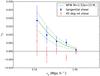 |
Fig. 20 Tangential shear signal as a function of radial separation. Errors are measured using 1000 bootstrap resamples. |
8. Kurk superstructure
CDF-S hosts over-densities of galaxies at z = 1.6 identified in the GMOS spectroscopic campaign (Kurk et al. 2009). Based on the deep X-ray data, we find that there are no obvious X-ray counterparts of them at a significant S/N. In Fig. 21, we present a detailed map around the over-dense region. All 5 putative peaks in the photo-z map of Kurk et al. (2009) are located within the area of positive X-ray flux with low S/N. But, as can be seen in the map, the X-ray emission from the over-densities, if any, would have been confused with nearby X-ray groups. While the detection of the sources is confused with foreground structure, it is still possible to perform the aperture fluxes, placing 30′′ aperture on each component. These sources have fluxes at or below 2 × 10-16 ergs s-1 cm-2. We include the properties of these sources in the main group catalog. As can be seen there, the putative groups typically have M200 ~ 2 × 10¹³M⊙. We note that the most massive X-ray selected system in the z = 1.6 structure is the Tanaka et al. (2013a) group with a mass of M200 ~ 3 × 10¹³M⊙. Given the spatial clustering of galaxies, the Kurk over-densities are likely a galaxy cluster in formation.
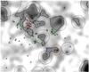 |
Fig. 21 Signal-to-noise map of X-ray residuals in the 0.5–2 keV band, after removing the point sources. The black circles show the location of the primary identifications. The solid red circle is the center of the Kurk superstructure and the solid green sources are other peaks on the photo-z at z = 1.6 with sufficient spectra and the blue circle is a photo-z peak with just one spectrum, all found in the map of Kurk et al. Small solid circles indicate the spectroscopic members of the 1.6 wall and the dashed red circle is the highest significance X-ray source at z = 1.6 presented in Tanaka et al. (2013). The radii of the circles correspond to R200, also giving a sense of the angular/physical scale (e.g. Tanaka’s group has a radii of 0.7′), with the coordinates of the circle centers listed in Table 4. |
9. Discussion and conclusion
We have presented the detection, identification and analysis of the extended sources in the deepest X-ray survey to date – the ECDF-S. After the careful subtraction of point-like sources in the XMM and Chandra data, we extract extended sources in the combined X-ray data. The optical counterparts of these sources are searched for using the red sequence technique with the deep, multi-wavelength data available in the field. A large combined effort of spectroscopic follow-up observations allowed us to derive spectroscopic redshifts of a large fraction of the systems.
The group catalog contains low-luminosity groups that can only be found in deep X-ray surveys. By means of stacked weak lensing as well as clustering, we have confirmed that these low-luminosity systems are indeed low-mass systems.
According to the hierarchical model of structure formation, massive galaxies spend most of their lifetime in group-sized halos (e.g. De Lucia et al. 2012) where environmental processes can strongly affect their evolution. Moreover, in the local Universe, groups represent the most common environment of galaxies (Geller & Huchra 1983; Eke et al. 2005). Therefore, studying galaxy groups at different cosmic times is vital to understand how the environment affects galaxy properties (e.g. star formation activity and morphology). ECDF-S catalog has already been exploited for the galaxy evolution as well as AGN studies Silverman et al. (2010), Popesso et al. (2012), Ziparo et al. (2013, 2014).
The CDFS group catalog presented in this work has already been crucial to underline the importance of groups with respect to other environments. For example, Ziparo et al. (2013) show that, opposite to what it is expected for clusters, groups lack of any radial trend in galaxy star formation. Nevertheless, the star formation activity in galaxy groups is globally suppressed with respect to group-like density regions and the field (Ziparo et al. 2014), suggesting that processes related to a group-sized dark matter halos are more efficient in quenching star formation than purely density related processes. Ziparo et al. (2014) also show that X-ray detected groups exhibit the fastest evolution in star formation activity, confirming the key role of pre-processing (Zabludoff & Mulchaey 1998) in the cosmic decline of star formation.
The properties of the identified groups such as mass-redshift distribution are broadly consistent with the Plank13 cosmology. There is a lack of structure in the ECDF-S at 0.2 < z < 0.5, while at other redshifts ECDF-S can be considered as a representative field. The field can be well described by the non-evolving XLF, which predicts 500 groups per square degree at 10-16 ergs s-1 cm2 flux limit.
Our successful extended source detections in the ECDF-S paves the way for future large area X-ray missions, such as Athena and WFXT, providing a realistic input for the modelling of source detection. Our experience shows that the point source removal is not the major bottleneck and moderate spatial resolution (of e.g. 5′′) will be sufficient for that. The most important issue, however, is precise modelling of the unresolved background since the flux of extended sources is typically 10% of the background. Furthermore, faint sources are often confused by the outskirts of nearby extended sources. The removal of these extended fluxes is also important from the point of view of the unresolved Cosmic X-ray Background (Cappelluti et al. 2012), as it can otherwise be mistaken for the clustering signal of the WHIM. The precise modelling of the background will be a major challenge in the next generation X-ray surveys.
Online material
Catalog of the ECDF-S X-ray selected galaxy groups.
All observed values quoted through this paper, are calculated adopting a Λ CDM cosmological model, with Ho = 70 km s-1 Mpc-1, ΩM = 0.24, ΩΛ = 0.76 (but see the modelling for testing Planck cosmological parameters. We quote all X-ray fluxes in the [0.5−2] keV band and rest-frame luminosities in the [0.1−2.4] keV band and provide the confidence intervals on the 68% level. FK5 coordinates used throughout.
Acknowledgments
This work has been partially supported through a SAO grant SP1-12006B to UMBC. W.N.B. thanks Chandra grant SP1-12007A and NASA ADP grant NNX10AC99G. A.F. and V.A. wish to acknowledge Finnish Academy award, decision 266918. M.T. acknowledges support by KAKENHI No. 23740144. P.R. acknowledges a grant from the Greek General Secretariat of Research and Technology in the framework of the programme Support of Postdoctoral Researchers. A.C. and C.H. acknowledge support from the European Research Council under the EC FP7 grant number 240185. J.S.M. acknowledges partial support from Chandra grant SP1-12006A. C.S. acknowledges support by DLR grants 50QR1103 and 50QR0803. Y.Q.X. acknowledges support of the Thousand Young Talents program (KJ2030220004), the 973 Program (2015CB857004), the USTC startup funding (ZC9850290195), the National Natural Science Foundation of China (NSFC-11473026, 11421303), and the Strategic Priority Research Program “The Emergence of Cosmological Structures” of the Chinese Academy of Sciences (XDB09000000). F.E.B. acknowledges support from Basal-CATA PFB-06/2007, CONICYT-Chile (FONDECYT 1141218, ALMA-CONICYT 31100004, Gemini-CONICYT 32120003, “EMBIGGEN” Anillo ACT1101), and Project IC120009 “Millennium Institute of Astrophysics (MAS)” of Iniciativa Científica Milenio del Ministerio de Economía, Fomento y Turismo.
References
- Adami, C., Mazure, A., Pierre, M., et al. 2011, A&A, 526, A18 [NASA ADS] [CrossRef] [EDP Sciences] [Google Scholar]
- Allen, S. W., Rapetti, D. A., Schmidt, R. W., et al. 2008, MNRAS, 383, 879 [NASA ADS] [CrossRef] [Google Scholar]
- Allevato, V., Finoguenov, A., Cappelluti, N., et al. 2011, ApJ, 736, 99 [NASA ADS] [CrossRef] [Google Scholar]
- Allevato, V., Finoguenov, A., Hasinger, G., et al. 2012, ApJ, 758, 47 [NASA ADS] [CrossRef] [Google Scholar]
- Balestra, I., Mainieri, V., Popesso, P., et al. 2010, A&A, 512, A12 [NASA ADS] [CrossRef] [EDP Sciences] [Google Scholar]
- Bauer, F. E., Alexander, D. M., Brandt, W. N., et al. 2004, AJ, 128, 2048 [NASA ADS] [CrossRef] [Google Scholar]
- Baugh, C. M., & Efstathiou, G. 1994, MNRAS, 267, 323 [NASA ADS] [Google Scholar]
- Bertin, E., & Arnouts, S. 1996, A&AS, 117, 393 [NASA ADS] [CrossRef] [EDP Sciences] [Google Scholar]
- Bielby, R. M., Finoguenov, A., Tanaka, M., et al. 2010, A&A, 523, A66 [NASA ADS] [CrossRef] [EDP Sciences] [Google Scholar]
- Böhringer, H., Schuecker, P., Guzzo, L., et al. 2001, A&A, 369, 826 [NASA ADS] [CrossRef] [EDP Sciences] [Google Scholar]
- Brandt, W. N., & Hasinger, G. 2005, ARA&A, 43, 827 [Google Scholar]
- Brunner, H., Cappelluti, N., Hasinger, G., et al. 2008, A&A, 479, 283 [NASA ADS] [CrossRef] [EDP Sciences] [Google Scholar]
- Bruzual, G., & Charlot, S. 2003, MNRAS, 344, 1000 [NASA ADS] [CrossRef] [Google Scholar]
- Cappelluti, N., Ranalli, P., Roncarelli, M., et al. 2012, MNRAS, 427, 651 [NASA ADS] [CrossRef] [Google Scholar]
- Carlberg, R. G., Yee, H. K. C., Ellingson, E., et al. 1997, ApJ, 476, L7 [NASA ADS] [CrossRef] [Google Scholar]
- Connelly, J. L., Wilman, D. J., Finoguenov, A., et al. 2012, ApJ, 756, 139 [NASA ADS] [CrossRef] [Google Scholar]
- Cooper, M. C., Yan, R., Dickinson, M., et al. 2012, MNRAS, 425, 2116 [NASA ADS] [CrossRef] [Google Scholar]
- Davis, M., & Peebles, P. J. E. 1983, ApJ, 267, 465 [NASA ADS] [CrossRef] [Google Scholar]
- Dehghan, S., & Johnston-Hollitt, M. 2014, AJ, 147, 52 [NASA ADS] [CrossRef] [Google Scholar]
- Duffy, A. R., Schaye, J., Kay, S. T., & Dalla Vecchia, C. 2008, MNRAS, 390, L64 [NASA ADS] [CrossRef] [Google Scholar]
- Erfanianfar, G., Finoguenov, A., Tanaka, M., et al. 2013, ApJ, 765, 117 [NASA ADS] [CrossRef] [Google Scholar]
- Erfanianfar, G., Popesso, P., Finoguenov, A., et al. 2014, MNRAS, 445, 2725 [NASA ADS] [CrossRef] [Google Scholar]
- Fernández-Soto, A., Lanzetta, K. M., & Yahil, A. 1999, ApJ, 513, 34 [NASA ADS] [CrossRef] [Google Scholar]
- Finoguenov, A., Guzzo, L., Hasinger, G., et al. 2007, ApJS, 172, 182 [Google Scholar]
- Finoguenov, A., Connelly, J. L., Parker, L. C., et al. 2009, ApJ, 704, 564 [NASA ADS] [CrossRef] [Google Scholar]
- Finoguenov, A., Watson, M. G., Tanaka, M., et al. 2010, MNRAS, 403, 2063 [NASA ADS] [CrossRef] [Google Scholar]
- Gawiser, E., van Dokkum, P. G., Herrera, D., et al. 2006, ApJS, 162, 1 [NASA ADS] [CrossRef] [Google Scholar]
- George, M. R., Leauthaud, A., Bundy, K., et al. 2011, ApJ, 742, 125 [NASA ADS] [CrossRef] [Google Scholar]
- George, M. R., Leauthaud, A., Bundy, K., et al. 2012, ApJ, 757, 2 [NASA ADS] [CrossRef] [Google Scholar]
- Giacconi, R., Zirm, A., Wang, J., et al. 2002, ApJS, 139, 369 [NASA ADS] [CrossRef] [Google Scholar]
- Giavalisco, M., Ferguson, H. C., Koekemoer, A. M., et al. 2004, ApJ, 600, L93 [NASA ADS] [CrossRef] [Google Scholar]
- Giodini, S., Pierini, D., Finoguenov, A., et al. 2009, ApJ, 703, 982 [NASA ADS] [CrossRef] [Google Scholar]
- Giodini, S., Finoguenov, A., Pierini, D., et al. 2012, A&A, 538, A104 [NASA ADS] [CrossRef] [EDP Sciences] [Google Scholar]
- Grazian, A., Fontana, A., de Santis, C., et al. 2006, A&A, 449, 951 [NASA ADS] [CrossRef] [EDP Sciences] [Google Scholar]
- Henry, J. P., Salvato, M., Finoguenov, A., et al. 2010, ApJ, 725, 615 [NASA ADS] [CrossRef] [Google Scholar]
- Heymans, C., Brown, M. L., Barden, M., et al. 2005, MNRAS, 361, 160 [NASA ADS] [CrossRef] [Google Scholar]
- Heymans, C., Van Waerbeke, L., Bacon, D., et al. 2006, MNRAS, 368, 1323 [NASA ADS] [CrossRef] [Google Scholar]
- Hickox, R. C., & Markevitch, M. 2006, ApJ, 645, 95 [NASA ADS] [CrossRef] [Google Scholar]
- Hilton, M., Lloyd-Davies, E., Stanford, S. A., et al. 2010, ApJ, 718, 133 [NASA ADS] [CrossRef] [Google Scholar]
- Hoekstra, H., Franx, M., Kuijken, K., & Squires, G. 1998, ApJ, 504, 636 [NASA ADS] [CrossRef] [Google Scholar]
- Jelić, V., Smolčić, V., Finoguenov, A., et al. 2012, MNRAS, 423, 2753 [NASA ADS] [CrossRef] [Google Scholar]
- Kaiser, N., Squires, G., & Broadhurst, T. 1995, ApJ, 449, 460 [NASA ADS] [CrossRef] [Google Scholar]
- Koekemoer, A. M., Fruchter, A. S., Hook, R. N., & Hack, W. 2003, in HST Calibration Workshop: Hubble after the Installation of the ACS and the NICMOS Cooling System, eds. S. Arribas, A. Koekemoer, & B. Whitmore, 337 [Google Scholar]
- Koens, L. A., Maughan, B. J., Jones, L. R., et al. 2013, MNRAS, 435, 3231 [NASA ADS] [CrossRef] [Google Scholar]
- Kurk, J., Cimatti, A., Zamorani, G., et al. 2009, A&A, 504, 331 [NASA ADS] [CrossRef] [EDP Sciences] [Google Scholar]
- Landy, S. D., & Szalay, A. S. 1993, ApJ, 412, 64 [NASA ADS] [CrossRef] [Google Scholar]
- Lanzetta, K. M., Yahil, A., & Fernández-Soto, A. 1996, Nature, 381, 759 [NASA ADS] [CrossRef] [Google Scholar]
- Leauthaud, A., Finoguenov, A., Kneib, J.-P., et al. 2010, ApJ, 709, 97 [NASA ADS] [CrossRef] [Google Scholar]
- Leauthaud, A., George, M. R., Behroozi, P. S., et al. 2012, ApJ, 746, 95 [NASA ADS] [CrossRef] [Google Scholar]
- Lehmer, B. D., Brandt, W. N., Alexander, D. M., et al. 2005, ApJS, 161, 21 [NASA ADS] [CrossRef] [Google Scholar]
- Lidman, C., Rosati, P., Tanaka, M., et al. 2008, A&A, 489, 981 [NASA ADS] [CrossRef] [EDP Sciences] [Google Scholar]
- Lloyd-Davies, E. J., Romer, A. K., Mehrtens, N., et al. 2011, MNRAS, 418, 14 [NASA ADS] [CrossRef] [Google Scholar]
- Luo, B., Bauer, F. E., Brandt, W. N., et al. 2008, ApJS, 179, 19 [NASA ADS] [CrossRef] [Google Scholar]
- Luppino, G. A., & Kaiser, N. 1997, ApJ, 475, 20 [NASA ADS] [CrossRef] [Google Scholar]
- MacDonald, E. C., Allen, P., Dalton, G., et al. 2004, MNRAS, 352, 1255 [NASA ADS] [CrossRef] [Google Scholar]
- Maughan, B. J. 2007, ApJ, 668, 772 [NASA ADS] [CrossRef] [Google Scholar]
- Meurer, G. R., Lindler, D. J., Blakeslee, J., et al. 2003, in SPIE Conf. Ser. 4854, eds. J. C. Blades, & O. H. W. Siegmund, 507 [Google Scholar]
- Miller, N. A., Bonzini, M., Fomalont, E. B., et al. 2013, ApJS, 205, 13 [NASA ADS] [CrossRef] [Google Scholar]
- Mirkazemi, M., Finoguenov, A., Pereira, M. J., et al. 2015, ApJ, 799, 60 [NASA ADS] [CrossRef] [Google Scholar]
- Navarro, J. F., Frenk, C. S., & White, S. D. M. 1996, ApJ, 462, 563 [NASA ADS] [CrossRef] [Google Scholar]
- Oh, S., Mulchaey, J. S., Woo, J.-H., et al. 2014, ApJ, 790, 43 [NASA ADS] [CrossRef] [Google Scholar]
- Okabe, N., Zhang, Y.-Y., Finoguenov, A., et al. 2010, ApJ, 721, 875 [NASA ADS] [CrossRef] [Google Scholar]
- Pacaud, F., Pierre, M., Adami, C., et al. 2007, MNRAS, 382, 1289 [NASA ADS] [CrossRef] [Google Scholar]
- Paolillo, M., Schreier, E. J., Giacconi, R., Koekemoer, A. M., & Grogin, N. A. 2004, ApJ, 611, 93 [NASA ADS] [CrossRef] [Google Scholar]
- Pierre, M., Clerc, N., Maughan, B., et al. 2012, A&A, 540, A4 [NASA ADS] [CrossRef] [EDP Sciences] [Google Scholar]
- Planck Collaboration XXVI. 2014, A&A, 571, A26 [NASA ADS] [CrossRef] [EDP Sciences] [Google Scholar]
- Popesso, P., Biviano, A., Rodighiero, G., et al. 2012, A&A, 537, A58 [NASA ADS] [CrossRef] [EDP Sciences] [Google Scholar]
- Rafferty, D. A., Brandt, W. N., Alexander, D. M., et al. 2011, ApJ, 742, 3 [NASA ADS] [CrossRef] [Google Scholar]
- Ranalli, P., Comastri, A., Vignali, C., et al. 2013, A&A, 555, A42 [NASA ADS] [CrossRef] [EDP Sciences] [Google Scholar]
- Rix, H.-W., Barden, M., Beckwith, S. V. W., et al. 2004, ApJS, 152, 163 [NASA ADS] [CrossRef] [Google Scholar]
- Rosati, P., Borgani, S., & Norman, C. 2002, ARA&A, 40, 539 [NASA ADS] [CrossRef] [Google Scholar]
- Salvato, M., Ilbert, O., Hasinger, G., et al. 2011, ApJ, 742, 61 [NASA ADS] [CrossRef] [Google Scholar]
- Santini, P., Fontana, A., Grazian, A., et al. 2009, A&A, 504, 751 [NASA ADS] [CrossRef] [EDP Sciences] [Google Scholar]
- Schmid, C., Martin, M., Wilms, J., et al. 2010, in Multi-Wavelength Approach and Future Perspectives, AIP Conf. Proc., 1248, 591 [NASA ADS] [CrossRef] [Google Scholar]
- Sheth, R. K., Hui, L., Diaferio, A., & Scoccimarro, R. 2001, MNRAS, 325, 1288 [NASA ADS] [CrossRef] [Google Scholar]
- Silverman, J. D., Mainieri, V., Salvato, M., et al. 2010, ApJS, 191, 124 [NASA ADS] [CrossRef] [Google Scholar]
- Smolčić, V., Finoguenov, A., Zamorani, G., et al. 2011, MNRAS, 416, L31 [NASA ADS] [CrossRef] [Google Scholar]
- Strüder, L., Aschenbach, B., Bräuninger, H., et al. 2001, A&A, 375, L5 [NASA ADS] [CrossRef] [EDP Sciences] [Google Scholar]
- Tanaka, M., Kodama, T., Kajisawa, M., et al. 2007, MNRAS, 377, 1206 [NASA ADS] [CrossRef] [Google Scholar]
- Tanaka, M., Finoguenov, A., Mirkazemi, M., et al. 2013a, PASJ, 65, 17 [NASA ADS] [Google Scholar]
- Tanaka, M., Toft, S., Marchesini, D., et al. 2013b, ApJ, 772, 113 [NASA ADS] [CrossRef] [Google Scholar]
- Taylor, J. E., Massey, R. J., Leauthaud, A., et al. 2012, ApJ, 749, 127 [NASA ADS] [CrossRef] [Google Scholar]
- Turner, M. J. L., Abbey, A., Arnaud, M., et al. 2001, A&A, 365, L27 [NASA ADS] [CrossRef] [EDP Sciences] [Google Scholar]
- Vikhlinin, A., McNamara, B. R., Forman, W., et al. 1998, ApJ, 502, 558 [NASA ADS] [CrossRef] [Google Scholar]
- Vikhlinin, A., Burenin, R. A., Ebeling, H., et al. 2009, ApJ, 692, 1033 [NASA ADS] [CrossRef] [Google Scholar]
- Wright, C. O., & Brainerd, T. G. 2000, ApJ, 534, 34 [NASA ADS] [CrossRef] [Google Scholar]
- Xue, Y. Q., Luo, B., Brandt, W. N., et al. 2011, ApJS, 195, 10 [NASA ADS] [CrossRef] [Google Scholar]
- Ziparo, F., Popesso, P., Biviano, A., et al. 2013, MNRAS, 434, 3089 [NASA ADS] [CrossRef] [Google Scholar]
- Ziparo, F., Popesso, P., Finoguenov, A., et al. 2014, MNRAS, 437, 458 [NASA ADS] [CrossRef] [Google Scholar]
All Tables
All Figures
|
Fig. 1 Combined Chandra and XMM exposure map of ECDF-S area. The contours represent levels of 0.1, 1, 2, 4, 8 and 12 Ms effective Chandra ACIS-I on-axis exposure. |
| In the text | |
|
Fig. 2 Sensitivity of Chandra and XMM towards the detection of X-ray emission on 32′′ scales. Contours show the levels of 1.2,2,3, and 5 × 10-16 ergs s-1 cm-2 and provide the intensity scale in the image. Left: all Chandra observations. The sensitivity does not reach the deepest contour. Middle: All XMM observations. Right: Chandra plus XMM. |
| In the text | |
|
Fig. 3 Wavelet reconstruction of the XMM image on 32′′ − 128′′ scales without (left panel) and with (right panel) the flux removal coming from the wings of point sources. The number of apparent sources changes by a factor of 2. |
| In the text | |
|
Fig. 4 Simulated XMM mosaic image of point source and background emission in the ECDF-S. |
| In the text | |
|
Fig. 5 Simulated residuals after the point source removal and background subtraction. Contours show the detected X-ray emission. We identify three detected false sources (highlighted by dashed circles). None of these sources were identified as a galaxy group. |
| In the text | |
|
Fig. 6 Signal-to-noise of the XMM data after point source removal and smoothing with a 16′′ Gaussian kernel. The color bar shows the correspondence between the color and the significance of the emission, starting with white for −1σ. |
| In the text | |
|
Fig. 7 Left: XMM detection of extended emission on a 32 arcsec scale. Right: Chandra detection of extended emission on a 32 arcsec scale. Contours, which are the same in both panels, show the extended emission detected in the combined Chandra and XMM images on the 32 and 64 arcsec scales. Full ECDF-S field of 0.3 sq.degrees is shown. |
| In the text | |
|
Fig. 8 Flux comparison between Chandra and XMM within the area covered by the 4 Ms Chandra CDF-S. The solid line shows the 1:1 correspondence. 38 extended sources with significant flux measurement in both Chandra and XMM data are shown. The errors on XMM fluxes are similar to the plotted Chandra errors and are omitted from the plot for clarity. |
| In the text | |
|
Fig. 9 Distribution of core radii of the detected simulated extended sources. The shades show the detected sources in the “Confusion” run, with shades of grey illustrating the overlap of sources. The dashed and solid lines show the location of 90% and 50% detection completeness level. The core radii are uniquely determined by the mass and redshift of the halo, using the tabulations of Finoguenov et al. (2007). |
| In the text | |
|
Fig. 10 Distribution of the beta parameter of the detected simulated extended sources. The shades show the detected sources in the “Confusion” run, with shades of grey illustrating the overlap of sources. The dashed and solid lines show the location of 90% and 50% detection completeness level. The value of beta is uniquely determined by the mass and redshift of the halo, using the tabulations of Finoguenov et al. (2007). |
| In the text | |
|
Fig. 11 Flux-redshift plane of the ECDF-S sample (filled circles with error bars). The grey shades show the distribution of the parameters of the detected groups in simulations, with Planck cosmological parameters (Planck Collaboration XXVI 2014) and the scaling relations of Leauthaud et al. (2010) used. Due to the limited spatial scales used, at low redshifts the effective sensitivity towards the total flux is lower. The upper boundary on the flux distribution shows the combination of the ECDF-S survey volume and cosmology. The dashed and solid lines show the location of 90% and 50% detection completeness level. |
| In the text | |
|
Fig. 12 Luminosity-redshift sampling in the ECDF-S. Grey shadowing indicate the density of detected groups in simulations, with Planck cosmological parameters (Planck Collaboration XXVI 2014) and the scaling relations of Leauthaud et al. (2010) used. Solid circles show the parameters of ECDF-S groups. The dashed and solid lines show the location of 90% and 50% detection completeness level. |
| In the text | |
|
Fig. 13 Mass-redshift sampling in the ECDF-S. Definition of mass is done with respect to the mean density and is scaled by the Hubble constant. Grey shadowing indicate the density of detected groups in simulations, with Planck cosmological parameters (Planck Collaboration XXVI 2014) and the scaling relations of Leauthaud et al. (2010) used. Solid circles show the parameters of ECDF-S groups. The dashed and solid lines show the location of 90% and 50% detection completeness level. |
| In the text | |
|
Fig. 14 Wavelet reconstruction of the simulated image of extended emission in the ECDF-S area on scales of 0.5−2 arcmin. The contours of the observed X-ray emission on matched spatial scales are overlaid in black. Contours not aligned with simulated X-ray emission correspond to unidentified sources. The contours do not show the largest scales of the emission, but similarity between the model image and the S/N image in Fig. 6 is clear. |
| In the text | |
|
Fig. 15 Comparison of the mass-redshift sampling of the ECDF-S (filled black circles) and COSMOS (filled grey circles) X-ray group samples. Definition of mass with with respect to the critical density. The ECDF-S groups extend to much lower masses, while occupying a similar redshift range. An improvement in the mass sensitivity of the survey scales as exposure to the power of 3.3, so 30 times deeper data in ECDF-S results in a 3 times better mass limit. |
| In the text | |
|
Fig. 16 X-ray luminosity function of ECDF-S groups. Black dots show the measurement using the full field, while black crosses show the measurements excluding the central region where there is a low spatial density of groups. Gray crosses show the results from the COSMOS field. Dashed and dotted curves show the local XLF in the Northern and Southern Hemisphere, revealing an effect of sample variance, caused by small volumes probed by RASS at low group luminosities. |
| In the text | |
|
Fig. 17 log (N>S) − log (S) of X-ray groups. The grey curves show ECDF-S data and the 1σ envelope shown as dashed curves. The solid black curve shows the prediction of a non-evolving X-ray luminosity function from Rosati et al. (2002). The long-dashed line shows the simulated detected counts using Planck cosmology (Planck Collaboration XXVI 2014) and the Leauthaud et al. (2010) scaling relation. The dotted line, illustrates the effect on changing the normalisation of scaling relations by increasing the associated mass by 30%, allowed by our calibration at faint fluxes (below 10-15 ergs s-1 cm-2). |
| In the text | |
|
Fig. 18 dn/ dz/ dΩ [deg-2] distribution of the ECDF-S groups (black crosses). The prediction from the detailed detection simulation and Planck cosmology (Planck Collaboration XXVI 2014) is shown as solid grey curve and the effect of 30% change in the scaling relations is shown by the dashed grey curve. |
| In the text | |
|
Fig. 19 Projected autocorrelation function of X-ray galaxy groups in the ECDF-S. The red points show the results for all the groups and the black points again for groups but excluding the central area from both real and random catalogs. As we discuss in the text, we do not see any significant change in the results, after introducing the method for correcting the first order effects from cosmic variance. The dotted lines show the two-halo terms |
| In the text | |
|
Fig. 20 Tangential shear signal as a function of radial separation. Errors are measured using 1000 bootstrap resamples. |
| In the text | |
|
Fig. 21 Signal-to-noise map of X-ray residuals in the 0.5–2 keV band, after removing the point sources. The black circles show the location of the primary identifications. The solid red circle is the center of the Kurk superstructure and the solid green sources are other peaks on the photo-z at z = 1.6 with sufficient spectra and the blue circle is a photo-z peak with just one spectrum, all found in the map of Kurk et al. Small solid circles indicate the spectroscopic members of the 1.6 wall and the dashed red circle is the highest significance X-ray source at z = 1.6 presented in Tanaka et al. (2013). The radii of the circles correspond to R200, also giving a sense of the angular/physical scale (e.g. Tanaka’s group has a radii of 0.7′), with the coordinates of the circle centers listed in Table 4. |
| In the text | |
Current usage metrics show cumulative count of Article Views (full-text article views including HTML views, PDF and ePub downloads, according to the available data) and Abstracts Views on Vision4Press platform.
Data correspond to usage on the plateform after 2015. The current usage metrics is available 48-96 hours after online publication and is updated daily on week days.
Initial download of the metrics may take a while.