| Issue |
A&A
Volume 572, December 2014
|
|
|---|---|---|
| Article Number | A44 | |
| Number of page(s) | 39 | |
| Section | Atomic, molecular, and nuclear data | |
| DOI | https://doi.org/10.1051/0004-6361/201423622 | |
| Published online | 27 November 2014 | |
Laboratory characterization and astrophysical detection of vibrationally excited states of vinyl cyanide in Orion-KL⋆,⋆⋆
1 Centro de Astrobiología (CSIC-INTA), Departamento de Astrofísica Molecular, Ctra. de Ajalvir Km 4, 28850 Torrejón de Ardoz, Madrid, Spain
e-mail: This email address is being protected from spambots. You need JavaScript enabled to view it.
2 Institute of Physics, Polish Academy of Sciences, Al. Lotników 32/46, 02-668 Warszawa, Poland
3 Jet Propulsion Laboratory, California Institute of Technology, 4800 Oak Grove Dr., Pasadena, CA 91109, USA
4 Grupo de Espectroscopia Molecular (GEM), Unidad Asociada CSIC, Edificio Quifima, Laboratorios de Espectroscopia y Bioespectroscopia, Parque Cientfico UVa, Universidad de Valladolid, 47011, Valladolid, Spain
5 Department of Physics and Astronomy, University College London, Gower Street, London WC1E 6B, UK
6 NRAO, 520 Edgemont Road, Charlottesville, VA 22902, USA
7 Wright State University, 3640 Colonel Glenn Hwy, Dayton, OH 45435, USA
8 Ohio State University, 191 W. Wooddruff Ave., Columbus, OH 43210, USA
Received: 11 February 2014
Accepted: 12 July 2014
Abstract
Context. We perform a laboratory characterization in the 18–1893 GHz range and astronomical detection between 80–280 GHz in Orion-KL with IRAM-30 m of CH2CHCN (vinyl cyanide) in its ground and vibrationally excited states.
Aims. Our aim is to improve the understanding of rotational spectra of vibrationally excited vinyl cyanide with new laboratory data and analysis. The laboratory results allow searching for these excited state transitions in the Orion-KL line survey. Furthermore, rotational lines of CH2CHCN contribute to the understanding of the physical and chemical properties of the cloud.
Methods. Laboratory measurements of CH2CHCN made on several different frequency-modulated spectrometers were combined into a single broadband 50–1900 GHz spectrum and its assignment was confirmed by Stark modulation spectra recorded in the 18–40 GHz region and by ab-initio anharmonic force field calculations. For analyzing the emission lines of vinyl cyanide detected in Orion-KL we used the excitation and radiative transfer code (MADEX) at LTE conditions.
Results. Detailed characterization of laboratory spectra of CH2CHCN in nine different excited vibrational states: ν11 = 1, ν15 = 1, ν11 = 2, ν10 = 1 ⇔ (ν11 = 1,ν15 = 1), ν11 = 3/ν15 = 2/ν14 = 1, (ν11 = 1,ν10 = 1) ⇔ (ν11 = 2,ν15 = 1), ν9 = 1, (ν11 = 1,ν15 = 2) ⇔ (ν10 = 1,ν15 = 1) ⇔ (ν11 = 1,ν14 = 1), and ν11 = 4 are determined, as well as the detection of transitions in the ν11 = 2 and ν11 = 3 states for the first time in Orion-KL and of those in the ν10 = 1 ⇔ (ν11 = 1,ν15 = 1) dyad of states for the first time in space. The rotational transitions of the ground state of this molecule emerge from four cloud components of hot core nature, which trace the physical and chemical conditions of high mass star forming regions in the Orion-KL Nebula. The lowest energy vibrationally excited states of vinyl cyanide, such as ν11 = 1 (at 328.5 K), ν15 = 1 (at 478.6 K), ν11 = 2 (at 657.8 K), the ν10 = 1 ⇔ (ν11 = 1,ν15 = 1) dyad (at 806.4/809.9 K), and ν11 = 3 (at 987.9 K), are populated under warm and dense conditions, so they probe the hottest parts of the Orion-KL source. The vibrational temperatures derived for the ν11 = 1, ν11 = 2, and ν15 = 1 states are 252 ± 76 K, 242 ± 121 K, and 227 ± 68 K, respectively; all of them are close to the mean kinetic temperature of the hot core component (210 K). The total column density of CH2CHCN in the ground state is (3.0 ± 0.9) × 1015 cm-2. We report the detection of methyl isocyanide (CH3NC) for the first time in Orion-KL and a tentative detection of vinyl isocyanide (CH2CHNC). We also give column density ratios between the cyanide and isocyanide isomers, obtaining a N(CH3NC)/N(CH3CN) ratio of 0.002.
Conclusions. Laboratory characterization of many previously unassigned vibrationally excited states of vinyl cyanide ranging from microwave to THz frequencies allowed us to detect these molecular species in Orion-KL. Column density, rotational and vibrational temperatures for CH2CHCN in their ground and excited states, and the isotopologues have been constrained by means of a sample of more than 1000 lines in this survey.
Key words: ISM: abundances / ISM: molecules / stars: formation / line: identification / methods: laboratory: molecular / radio lines: ISM
The full Tables A.6–A.14 are only available at the CDS via anonymous ftp to cdsarc.u-strasbg.fr (130.79.128.5) or via http://cdsarc.u-strasbg.fr/viz-bin/qcat?J/A+A/572/A44
This work was based on observations carried out with the IRAM-30 m telescope. IRAM is supported by INSU/CNRS (France), MPG (Germany), and IGN (Spain).
© ESO, 2014
1. Introduction
The rotational spectrum of vinyl cyanide (CH2CHCN) was first studied in 1954 by Wilcox and collaborators and then later by Costain & Stoicheff (1959), who also investigated the singly-substituted 13C species, as well as the 15N, and the CH2CDCN species. This molecule was detected for the first time in the interstellar medium (ISM) in 1973 toward the Sagittarius B2 (Sgr B2) molecular cloud (Gardner & Winnewisser1975). Since then, CH2CHCN has been detected toward different sources, such as Orion (Schilke et al.1997), the dark cloud TMC-1 (Matthews & Sears1983), the circumstellar envelope of the late-type star IRC+10216 (Agúndez et al.2008), and the Titan atmosphere (Capone et al.1981). CH2CHCN is one of the molecules, whose high abundance and significant dipole moment allow radioastronomical detection even of its rare isotopologue species. Thus, vinyl cyanide makes an important contribution to the millimeter and submillimeter spectral emissions covered by high sensitivity facilities, such as ALMA and the Herschel Space Telescope. However, there has not yet been a comprehensive study of its low-lying vibrational excited states.
Vinyl cyanide is a planar molecule (six internuclear distances and five independent bond angles) and is a slightly asymmetric prolate rotor with two non-zero electric dipole moment components, which lead to a rich rotational spectrum. The first detailed discussion of the vinyl cyanide microwave spectrum was in 1973 by Gerry & Winnewisser. Subsequent studies of the rotational spectrum of vinyl cyanide resulted in the determination of its electrical dipole moment components by Stolze & Sutter (1985); these values were later improved by Krasnicki & Kisiel (2011) who reported the values μa = 3.821(3) D, μb = 0.687(8) D, and μTOT = 3.882(3) D. Additional studies upgraded the molecular structure as Demaison et al. (1994), Colmont et al. (1997), and Krasnicki et al. (2011) successively derived more refined structural parameters from the rotational constants. The 14N nuclear quadrupole hyperfine structure has been studied by Colmont et al. (1997), Stolze & Sutter (1985), and Baskakov et al. (1996).
Kisiel et al. (2009a) updated the rotational constants by simultaneously fitting the rotational lines of CH2CHCN in its ground and lowest excited state ν11 = 1. They fit the ground states of the 13C and the 15N isotopologues. More detailed analysis of the isotopologue spectra was later reported by Krasnicki et al. (2011). The ground state rotational a-type and b-type transitions of the parent vinyl cyanide have been assigned up to J = 129 with measurements in the laboratory reaching 1.67 THz (Kisiel et al.2009a). They showed the influence of temperature on the partition function and consequently on the spectrum of vinyl cyanide. Figure 1 of Kisiel et al. (2009a) identifies this effect and the dominance of the millimeter and submillimeter region by the aR-type transitions. However, the b-type R-branch rotational transitions are one order of magnitude more intense than those of a-type due to smaller values of the rotational quantum numbers J at high frequencies (THz region).
The rotational transitions of CH2CHCN in several of the lowest vibrational excited states, ν11 = 1,2,3 and ν15 = 1, were assigned by Cazzoli & Kisiel (1988), and the measurements were extended by Demaison et al. (1994) (ν11 = 1 and the ground state). The data for ν11 = 3 was more limited by hindering the determination of all sextic or even quartic constants. Recently, the analysis of broadband rotational spectra of vinyl cyanide revealed that there are perturbations between all pairs of adjacent vibrational states extending upwards from the ground state (g.s.), see Fig. 2 of Kisiel et al. (2009a). Kisiel et al. (2012) covered a broader frequency region (90–1900 GHz) identifying and fitting the perturbations in frequencies of rotational transitions due to a-, b- or c-axis Coriolis-type or Fermi type interactions between the four lowest states of vinyl cyanide (g.s., ν11 = 1, ν15 = 1, and ν11 = 2). The need for perturbation treatment of the ν10/ν11ν15 dyad at about 560 cm-1 and the 3ν11/2ν15/ν14 triad of states at about 680 cm-1 was also identified, and initial results for the dyad were reported in Kisiel et al. (2011). Thus a meticulous analysis aiming toward an eventual global fit of transitions in all states of vinyl cyanide is necessary. The low resolution, gas-phase infrared spectrum of vinyl cyanide and its vibrational normal modes were studied by Halverson et al. (1948) and by Khlifi et al. (1999). Partial rotational resolution of the vibration-rotation spectrum of the two lowest wavenumber modes was also reported in the far-infrared study by Cole & Green (1973).
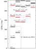 |
Fig. 1 All vibrational levels of vinyl cyanide up to 1000 cm-1. The levels in red are those for which rotational transitions have been analyzed in this work. The boxes identify sets of levels treated by means of coupled fits accounting for interstate perturbations. |
The first detection in the ISM of vinyl cyanide was in 1973 by means of the 211–212 line in emission in Sgr B2 and was confirmed in 1975 by Gardner & Winnewisser (1975), suggesting the presence of the simplest olefin in the ISM, CH2=CH2 (ethylene) based on the evidence of the reactive vinyl radical. Betz (1981) observed the non-polar organic molecule CH2=CH2 toward the red giant C-rich star IRC+10216, for the first time; specifically, this is the ν7 band in the rotation-vibration spectral region (28 THz). Owing to the symmetry of ethylene the dipole rotational transitions are forbidden, and Occhiogroso et al. (2013) estimated a column density of 1.26 × 1014 cm-2 in standard hot cores for this molecule based on the abundance of its derivative molecule, hydrocarbon methylacetylene (CH3CCH).
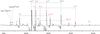 |
Fig. 2 Room-temperature laboratory spectrum of vinyl cyanide in the region of the 413 − 312 rotational transition recorded with a Stark modulation spectrometer. All marked lines are for the 413 − 312 transition in a given vibrational or isotopic species and display a characteristic pattern of negative lobes due to the non-zero field cycle of Stark modulation. Dotted lines connect vibrational states analyzed as perturbing polyads, red denotes vibrational states analyzed in the present work, and asterisks identify states detected presently in Orion-KL. It can be seen that laboratory analysis is now available for excited vibrational state transitions that are comparable in room-temperature intensity to those for 13C isotopologues in terrestrial natural abundance. |
The dense and hot molecular clouds, such as Orion and Sgr B2, give rise to emission lines of vibrationally excited states of vinyl cyanide. Rotational transitions in the two lowest frequency modes ν11 and ν15 were detected in Orion by Schilke et al. (1997) (as tentative detection of three and two lines, respectively) and in Sgr B2 by Nummelin & Bergman (1999) (64 and 45 identified lines, respectively). The latter authors also made the tentative detection transitions in the 2ν11 mode (five lines). Recently, Belloche et al. (2013) detected six vibrational states in a line survey of Sgr B2(N) (ν11 = 1, 2, 3,ν15 = 1, 2, ν11 = ν15 = 1) among which they detected the higher-lying vibrational states for the first time in space.
On the other hand, the ground states of rare isotopologues have been well characterized in the laboratory (Colmont et al.1997; Müller et al.2008; Kisiel et al.2009a; Krasnicki et al.2011). All monosubstituted species containing 13C, 15N, and D, and those of all 13C-monosubstituted species of H2C=CDCN of both cis- and trans- conformers of HDC=CHCN, HDC=CDCN, and D2C=CDCN have been characterized. The double 13C and 13C15N species have also been assigned by Krasnicki et al. (2011). The detection of 13C species of vinyl cyanide in the ISM was carried out toward Sgr B2 by Müller et al. (2008) with 26 detected features.
Spectroscopic data sets for excited vibrational states of CH2CHCN acquired in this work.
The millimeter line survey of Orion-KL carried out with the IRAM-30 m telescope by Tercero and collaborators (Tercero et al.2010, 2011; Tercero2012) presented 8000 unidentified lines initially. Many of these features (near 4000) have been subsequently identified as lines arising from isotopologues, and vibrationally excited states of abundant species, such as ethyl cyanide and methyl formate, thanks to a close collaboration with different spectroscopic laboratories (Demyk et al.2007; Margulès et al.2009; Carvajal et al.2009; Margulès et al.2010; Tercero et al.2012; Motiyenko et al.2007; Daly et al.2013; Coudert et al.2013; Haykal et al.2014). In this work, we followed the procedure of our previous papers, searching for all isotopologues and vibrationally excited states of vinyl cyanide in this line survey. These identifications are essential to probe new molecular species which reduce the number of U-lines and help to reduce the line confusion in the spectra. At this point we were ready to begin the search for new molecular species in this cloud by providing clues to the formation of complex organic molecules on the grain surfaces and/or in the gas phase (see the discovery of methyl acetate and gauche ethyl formate in Tercero et al.2013, the detection of the ammonium ion in Cernicharo et al.2013, and the first detection of ethyl mercaptan in Kolesniková et al.2014).
We report extensive characterization of 9 different excited vibrational states of vinyl cyanide (see Fig. 1) positioned in energy immediately above ν11 = 2, which, up to this point, has been the highest vibrational state subjected to a detailed study (Kisiel et al.2012). The assignment is confirmed by using the Stark modulation spectrometer of the spectroscopic laboratory (GEM) of the University of Valladolid and ab initio calculations. The new laboratory assignments of ν11 = 2, ν11 = 3, and ν10 = 1 ⇔ (ν11 = 1,ν15 = 1) vibrational modes of vinyl cyanide were used successfully to identify these three states in Orion-KL; the latter for the first time in the ISM. We also detected the ν11 = 1 and ν15 = 1 excited states in Orion-KL, as well as the ground state, and the 13C isotopologues (see Sect. 4.2.1).
Because isomerism is a key issue for a more accurate understanding of the formation of interstellar molecules, we report observations of some related isocyanide isomers. Bolton et al. (1970) carried out the first laboratory study of the pure rotation (10–40 GHz) spectrum of vinyl isocyanide and also studied its 200–4400 cm-1 vibrational spectrum. Laboratory measurements were subsequently extended up to 175 GHz by Yamada & Winnewisser (1975) and the hyperfine structure of cm-wave lines was measured by Bestmann & Dreizler (1982). In Sect. 4.5, we searched for all isocyanides corresponding to the detected cyanides in Orion-KL: methyl cyanide (Bell et al.2014), ethyl cyanide (Daly et al.2013), cyanoacetylene (Esplugues et al.2013b), cyanamide, and vinyl cyanide. In this study, we have tentatively detected vinyl isocyanide (CH2CHNC) in Orion-KL (see Sect. 4.5). In addition, we observed methyl isocyanide (CH3NC) for the first time in Orion-KL, which was observed firstly by Cernicharo et al. (1988) in the Sgr B2(OH) source, and we provide a tentative detection of ethyl isocyanide and isomers HCCNC and HNCCC of isocyanoacetylene. After the detection of cyanamide (NH2CN) by Turner et al. (1975) in Sgr B2, we report the tentative detection of this molecule in Orion, as well as a tentative detection for isocyanamide.
Finally, we discuss and summarize all results in Sects. 5 and 6.
2. Experimental
The present spectroscopic analysis is based largely on the broadband rotational spectrum of vinyl cyanide compiled from segments recorded in several different laboratories. That spectrum provided a total of 1170 GHz of coverage and its makeup was detailed in Table 1 of Kisiel et al. (2012). In the present work, the previous spectrum has been complemented by two additional segments: 50–90 GHz and 140–170 GHz recorded at GEM by using cascaded multiplication of microwave synthesizer output. The addition of these segments provides practically uninterrupted laboratory coverage of the room-temperature rotational spectrum of vinyl cyanide over the 50–640 GHz region, which is key to the analysis of vibrational state transitions.
Another laboratory technique brought in by GEM is Stark spectroscopy at cm-wave frequencies. The Stark-modulation technique has the useful property of preferentially recording a given low-J rotational transition by a suitable choice of the modulation voltage. This is particularly the case for the lowest-J, Ka = 1 transitions. Due to asymmetry splitting, these transitions are significantly shifted in frequency relative to other transitions for the same J value. An example spectrum of this type is shown in Fig. 2 where all, but some of the weakest lines, correspond to the 413 − 312 transition in either a vibrational state of the parent vinyl cyanide or the ground state of an isotopic species. Such spectra are particularly useful for an initial assignment since vibrationally induced frequency differences from the ground state are near additive. Relative intensities of transitions also give an immediate measure of relative population of assigned vibrational states and isotopic species.
The analysis of the spectra was carried out with the AABS graphical package for Assignment and Analysis of Broadband Spectra (Kisiel et al.2005, 2012), which is freely available on the PROSPE database (Kisiel, 2001)1. The AABS package was complemented by the SPFIT/SPCAT program package (Pickett1991)2 used for setting up the Hamiltonian, fitting, and prediction.
Supporting ab initio calculations were carried out with GAUSSIAN 093 and CFOUR4 packages. The key parameters for vibrational assignment are vibrational changes in rotational constants, which require relatively lengthy anharmonic force field calculations. Two strategies were used for this purpose: a relatively long basis set combined with a basic electron correlation correction (MP2/6-311++G(d,p)) and a more thorough correlation correction with a relatively simple basis set (CCSD(T)/ 6-31G(d,p)). The final results minimally favored the second approach but, in practice, both were found to be equally suitable.
3. Laboratory spectroscopy
3.1. Analysis of the excited vibrational states
An overview of the results of the spectroscopic analysis is provided in Table 1 and the determined spectroscopic constants necessary for generating linelists are given in Tables 2 and A.1–A.4.
Spectroscopic constants in the diagonal blocks of the Hamiltonian for the ν10 ⇔ ν11ν15 and the ν11ν10 ⇔ 2ν11ν15 dyads of vibrational states in vinyl cyanide compared with those for the ground state.
The initial assignment was based on a combination of several techniques: (1) inspection of Stark spectra such as that in Fig. 2; (2) the use of the concept of harmonic behavior of rotational constant changes on vibrational excitation (linear additivity of changes); and (3) ab initio calculations of vibration-rotation constants. The final assignment of vibrational states is confirmed by the comparison of values of experimental vibration-rotation changes in rotational constants relative to the ground state with computed ab initio values, as listed in Table A.5.
Preliminary studies revealed a multitude of perturbations in rotational frequencies that necessitate the use of fits that account for interactions between vibrational states. The grouping of energy levels visible in Fig. 1 suggests that it was possible to break the treatment down into three isolated polyads above the last state studied in detail, namely 2ν11. The symmetry classification of vibrational states (A′ and A′′, Cs point group) is marked in Fig. 1 and states of different symmetry need to be connected by a- and b-type Coriolis interactions, while states of the same symmetry are coupled via c-type Coriolis and Fermi interactions. The Hamiltonian and the techniques of analysis used to deal with this type of problem have been described in detail in Kisiel et al. (2009a, 2012). This type of analysis is far from trivial, but its eventual success for the polyads near 560, 680, and 790 cm-1 is confirmed in Table 1 by the magnitudes of the deviations of fit in relation to the numbers of fitted lines and their broad frequency coverage. In the most extensive of the present analyses, for the ν10 = 1 ⇔ (ν11 = 1,ν15 = 1) dyad, the fit encompasses almost 4000 lines in addition to aR-type transitions that include bQ- and bR-types. We use the 10σ cutoff criterion of SPFIT to prevent lines perturbed by factors outside the model from unduly affecting the fit, and a moderate number of such lines (191) are rejected for this dyad. These are confidently assigned lines, generally in high-J tails of some transition sequences for higher values of Ka, but their incompatibility suggests that there is hope for a final global fit with coupling between the polyads. At the present stage, the success of the perturbation fits is further reflected by additive vibrational changes in values of quartic centrifugal distortion constants and by the relative changes in perturbation constants between the two dyads listed in Table A.2, which are similar to those found for the well studied case of ClONO2 (Kisiel et al.2009b).
Unlike the situation in the ground state of vinyl cyanide (Kisiel et al.2009a), the perturbations visible in the presently studied polyads are not a spectroscopic curiosity but affect the strongest, low-Ka, aR-type transitions. Such transitions occur in the mm- and submm-wave regions which are normally the choice for astrophysical studies. This effect is illustrated by the scaled plots in Fig. 3, which would have the form of near horizontal, very smoothly changing lines in the absence of perturbations. Perturbations lead to the marked spike shaped features in these plots. Since evaluation of the Hamiltonian is made in separate blocks for each value of J, the perturbations affecting the two coupling states should have a mirror image form, as seen in Fig. 3. The scaled nature of these plots hides the reason that perturbations to the frequencies of many lines are considerable. For example, the peak of the rightmost spike in Fig. 3 corresponds to a perturbation shift of close to 50 × 64 MHz, namely 3.2 GHz. The frequencies of aR-transitions corresponding to the maximum perturbation peaks visible in Fig. 3 are 154.1, 183.4, 301.4, 456.5, and 620.8 GHz for ν10, and 131.9, 174.9, 290.3, 443.3, 604.9 GHz for ν11ν15. A significant number of transitions around such peaks are also clearly perturbed. The perturbations are not limited to frequency but also extend to intensities, which are often significantly decreased for pure rotation transitions near the perturbation maxima. The considerable energy level mixing in these cases leads instead to the appearance of transitions between the perturbing vibrational states. These transitions could only be predicted accurately in the final stages of the perturbation analysis but were easily found in the compiled broadband laboratory spectrum and are explicitly identified in the data files. Fortunately, the line lists generated from perturbation fits with the use of the SPCAT program reflect both frequency and intensity perturbations. Accounting for such effects at laboratory experimental accuracy is therefore the key to successful astrophysical studies.
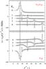 |
Fig. 3 Effect of vibration-rotation perturbations on frequencies of the strongest rotational transitions in the ν10 ⇔ ν11ν15 dyad of vibrational states. The plotted quantities are scaled frequency differences relative to the same transitions in the ground state. Continuous lines are predictions from the final fit; circles mark assigned lines and traces in each panel have added vertical shifts to improve clarity. |
Above the ν10ν11 ⇔ 2ν11ν15 dyad, the density of vibrational states rapidly increases. The complexity of a thorough analysis appears to be too forbidding at this stage, but it is possible to check how successfully some of these states can be encompassed by single state, effective fits. The ν9 vibrational state seems to be the most isolated, and its analysis could be taken up to Ka = 7 and transition frequencies of 570 GHz. In contrast, the easy to locate 4ν11 state exhibited very incomplete sequences of transitions even at low values of Ka, so that its analysis could only be taken up to Ka = 5. The very fragmentary nature of line sequences for this state illustrates the limitations of single state approaches, but it nevertheless provides a useful starting point for any future work. The complete results of fit and the primary data files for the SPFIT program for all coupled and single-state effective fits are available online5, while the predicted linelists will be incorporated in the JPL database.
3.2. Vibrational energies
In Table 1 we report a consistent set of vibrational energies for the studied excited states of vinyl cyanide, which are evaluated by taking advantage of results from the various perturbation analyses. The values for 3ν11 and 4ν11 are from ν11 and the anharmonicity coefficient x11,11 from Kisiel et al. (2012). The value for ν11ν15 comes from ν11 and ν15 augmented by x11,15, which is calculated at the CCSD(T)/cc-PVDZ level that was benchmarked in Kisiel et al. (2012) as the optimum level for evaluating this type of constant for vinyl cyanide. The remaining vibrational energies in the lower dyad, and the triad are evaluated using the precise ΔE values from the perturbation analyses. Finally, ν10ν11 comes from ν10 and ν11 augmented by ab initio x10,11. A double check of this procedure is provided by an alternative evaluation for 2ν15 based on ab initio x15,15, which gives a result within 0.5 cm-1 of the more reliable tabulated value. Only the vibrational energy for ν9 comes from the low resolution gas phase infrared spectrum (Halverson et al.1948).
4. Astronomical detection of vinyl cyanide species
Thanks to these new laboratory data, we identified and detected the ν10 = 1 ⇔ (ν11 = 1,ν15 = 1) vibrational modes of CH2CHCN for the first time in space. A consistent analysis of all detected species of vinyl cyanide have been made to outline the knowledge of our astrophysical environment. We also report the detection of methyl isocyanide for the first time in Orion KL and a tentative detection of vinyl isocyanide and calculate abundance ratios between the cyanide species and their corresponding isocyanide isomers.
4.1. Observations and overall results
4.1.1. 1D Orion-KL line survey
The line survey was performed over three millimeter windows (3, 2, and 1.3 mm) with the IRAM-30 m telescope (Granada, Spain). The observations were carried out between September 2004 and January 2007 pointing toward the IRc2 source at α2000.0 = 5h35m14.5s and δ2000.0 = −5°22′30.0′′. All the observations were performed using the wobbler switching mode with a beam throw in azimuth of ±120′′. System temperatures were in the range of 100–800 K from the lowest to the highest frequencies. The intensity scale was calibrated using the atmospheric transmission model (ATM, Cernicharo1985; Pardo et al.2001a). Focus and pointing were checked every 1–2 h. Backends provided a spectrum of 1–1.25 MHz of spectral resolution. All spectra were single-side band reduced. For further information about observations and data reduction, see Tercero et al. (2010)6.
All figures are shown in main beam temperature (TMB) that is related to the antenna temperature ( ) by the equation:
  /ηMB, where ηMB is the main beam efficiency which depends on the frequency.
According to previous works, we characterize at least four different cloud components overlapping in the beam in the analysis of low angular resolution line surveys of Orion-KL (see, e.g., Blake et al.1987, 1996; Tercero et al.2010, 2011): (i) a narrow (~4 km s-1 line-width) component at vLSR ≃ 9 km s-1 delineating a north-to-south extended ridge or ambient cloud or an extended region with Tk ≃ 60 K, n(H2) ≃ 105 cm-3; (ii) a compact (dsou ≃ 15′′) and quiescent region, or the compact ridge, (vLSR ≃ 7–8 km s-1, Δv ≃ 3 km s-1, Tk ≃ 150 K, n(H2) ≃ 106 cm-3); (iii) the plateau, or a mixture of outflows, shocks, and interactions with the ambient cloud (vLSR ≃ 6–10 km s-1, Δv ≳ 25 km s-1, Tk ≃ 150 K, n(H2) ≃ 106 cm-3, and dsou ≃ 30′′); (iv) a hot core component (vLSR ≃ 5 km s-1, Δv ≃ 5–15 km s-1, Tk ≃ 250 K, n(H2) ≃ 5 × 107 cm-3, and dsou ≃ 10′′). Nevertheless, we found a more complex structure of that cloud (density and temperature gradients of these components and spectral features at a vLSR of 15.5 and 21.5 km s-1 related with the outflows) in our analysis of different families of molecules (see, e.g., Tercero et al.2011; Daly et al.2013; Esplugues et al.2013a).
4.1.2. 2D survey observations
We also carried out a two-dimensional line survey with the same telescope in the ranges 85−95.3, 105−117.4, and 200.4−298 GHz (N. Marcelino et al. priv. comm.) during 2008 and 2010. This 2D survey consists of maps of 140 × 140 arcsec2 area with a sampling of 4 arcsec using a On-The-Fly mapping mode with a reference position 10 arcmin west of Orion-KL. The EMIR heterodyne receivers were used for all the observations except for 220 GHz frequency setting, for which the HERA receiver array was used. As backend, we used the WILMA backend spectrometer for all spectra (bandwidth of 4 GHz and 2 MHz of spectral resolution) and the FFTS (Fast Fourier Transform Spectrometer, 200 kHz of spectral resolution) for frequencies between 245−259, 264.4−278.6, and 289–298 GHz. Pointing and focus were checked every 2 h giving errors less than 3 arcsec. The data were reduced using the GILDAS package7 by removing bad pixels, checking for image sideband contamination and emission from the reference position, and fitting and removing first order baselines. Six transitions of CH2CHCN have been selected to study the spatial extent of their emission with this 2D line survey.
4.2. Results
4.2.1. Detection of CH2CHCN: its vibrationally excited states and its isotopologues in Orion-KL
Vinyl cyanide shows emission from a large number of rotational lines through the frequency band 80–280 GHz. The dense and hot conditions of Orion-KL populate the low-lying energy excited states. Here, we present the first interstellar detection of the ν10 = 1⇔(ν11 = 1,ν15 = 1) vibrational excited state.
Figures 4−8 and A.1 show selected detected lines of the g.s. of vinyl cyanide and five vibrationally excited states of the main isotopologue CH2CHCN: in plane C-C≡N bending mode (ν11 = 1, 228.1 cm-1 or 328.5 K), out of plane C-C≡N bending mode (ν15 = 1, 332.7 cm-1 or 478.6 K), in plane C-C≡N bending mode (ν11 = 2, 457.2 cm-1 or 657.8 K), in a combination state (ν10 = 1⇔(ν11 = 1,ν15 = 1), 560.5/562.9 cm-1 or 806.4/809.9 K), and in plane C-C≡N bending mode (ν11 = 3, 686.6 cm-1 or 987.9 K). The latter is in the detection limit, so we do not address the perturbations of this vibrational mode.
 |
Fig. 4 Observed lines from Orion-KL (histogram spectra) and model (thin red curves) of vinyl cyanide in the ground state. The cyan line corresponds to the model of the molecules we have already studied in this survey (see text Sect. 4.4.2), including the CH2CHCN species. A vLSR of 5 km s-1 is assumed. |
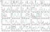 |
Fig. 5 Observed lines from Orion-KL (histogram spectra) and model (thin red curves) of CH2CHCN of ν11 = 1. The cyan line corresponds to the model of the molecules we have already studied in this survey (see text Sect. 4.4.2), including the CH2CHCN species. A vLSR of 5 km s-1 is assumed. |
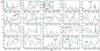 |
Fig. 6 Observed lines from Orion-KL (histogram spectra) and model (thin red curves) for the ν15 = 1 vibrational state of CH2CHCN. The cyan line corresponds to the model of the molecules we have already studied in this survey (see text Sect. 4.4.2), including the CH2CHCN species. A vLSR of 5 km s-1 is assumed. |
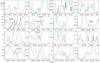 |
Fig. 7 Observed lines from Orion-KL (histogram spectra) and model (thin red curves) for the ν11 = 2 vibrational state of CH2CHCN. The cyan line corresponds to the model of the molecules we have already studied in this survey (see text Sect. 4.4.2), including the CH2CHCN species. A vLSR of 5 km s-1 is assumed. |
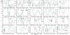 |
Fig. 8 Observed lines from Orion-KL (histogram spectra) and model (thin red curves) for combined vibrationally excited states of CH2CHCN in the ν10 = 1 ⇔ (ν11 = 1, ν15 = 1) dyad. The cyan line corresponds to the model of the molecules we have already studied in this survey (see text Sect. 4.4.2), including the CH2CHCN species. A vLSR of 5 km s-1 is assumed. |
 |
Fig. 9 Observed lines from Orion-KL (histogram spectra) and model (thin red curves) of 13C isotopes for CH2CHCN in the ground state. The subindex in 13Ci (i = 1, 2, 3) corresponds to the position of the isotope in the molecule (i1CH |

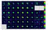 |
Fig. 10 Integrated intensity maps for 6 ground state transitions of vinyl cyanide. From line 1 (top row) to 6 (bottom row): 121,12–111,11 (110 839.98 MHz, 36.8 K), 240,24–230,23 (221 766.03 MHz, 134.5 K), 242,23–232,22 (226 256.88 MHz, 144.8 K), 261,26–251,25 (238 726.808 MHz, 157.4 K), 262,25–252,24 (244 857.47 MHz, 167.9 K), and 2410,15–2310,14 and 2410,14–2310,13 (228017.34 MHz, 352.0 K) at different velocity ranges (indicated in the top of each column). Three boxes have been blanked because the emission at these velocities was blended with that from other well known species. For each box axis are in units of arcseconds (Δα, Δδ). Color logarithm scale is the integrated intensity ( |

In addition, we detected the following isotopologues of vinyl cyanide in its ground state: 13CH2CHCN, CH213CHCN, and CH2CH13CN (see Fig. 9). For CH2CHC15N and the deuterated species of vinyl cyanide, DCHCHCN, HCDCHCN, and CH2CDCN (see Fig. A.2), we only provided a tentative detection in Orion-KL because of the small number of lines with an uncertainty in frequency less than 2 MHz (up to Ka = 7, 5, 15 for DCHCHCN, HCDCHCN, and CH2CDCN, respectively), the weakness of the features, and/or their overlap with other molecular species.
Tables A.6−A.13 show observed and laboratory line parameters for the ground state, the vibrationally excited states, and the 13C-vinyl cyanide isotopologues. Spectroscopic constants were derived from a fit with the MADEX code (Cernicharo2012) to the lines reported by Kisiel et al. (2009a, 2012), Cazzoli & Kisiel (1988), and Colmont et al. (1997). For the ν10 = 1 ⇔ (ν11 = 1, ν15 = 1) state, spectroscopic constants are those derived in this work; dipole moments were from Krasnicki & Kisiel (2011). All these parameters have been implemented in MADEX to obtain the predicted frequencies and the spectroscopic line parameters. We have displayed rotational lines that are not strongly overlapped with lines from other species. Observational parameters have been derived by Gaussian fits (using the GILDAS software) to the observed line profiles that are not blended with other features. For moderately blended and weak lines, we show observed radial velocities and intensities given directly from the peak channel of the line in the spectra, so contribution from other species or errors in baselines could appear for these values. Therefore, the main beam temperature for the weaker lines (TMB< 0.1 K) must be considered as an upper limit.
From the derived Gaussian fits, we observe that vinyl cyanide lines reflect the spectral line parameters corresponding to hot core/plateau components (vLSR between 2–3 km s-1 for the component of 20 km s-1 of line width, and 5–6 km s-1 for the component of 6 km s-1 of line width). As shown by Daly et al. (2013) there is a broad component associated to the hot core that limits the accuracy of the derived velocities for the hot core and this broad component. Our velocity components for CH2CHCN agree with those of CH3CH2CN obtained by Daly et al. (2013). Besides, for the vibrationally excited states, we found contribution of a narrow component with a vLSR of 3–6 km s-1 and a line width of ≃7 km s-1.
We rely on catalogs8 to identify possible contributions from other species overlapping the detected lines (Tercero2012), but it should be necessary to perform radiative transfer modeling with all the known molecules in order to precisely assess how much the contamination from other species influences the vinyl cyanide lines.
Number of identified lines of CH2CHCN species.
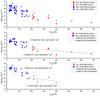 |
Fig. 11 Rotational diagram of CH2CHCN in its ground state. The upper panel displays the two components derived from the line profiles. The middle panel shows two linear fits to the narrow component points; these linear regressions yield temperatures and column densities of Trot = 125 ± 16 K and N = (1.3 ± 0.1) × 1015 cm-2 (Qrot = 7.06 × 10³), and Trot = 322 ± 57 K and N = (1.0 ± 0.2) × 1015 cm-2 (Qrot = 2.92 × 10⁴). Likewise, the bottom panel shows another two linear fits to the points corresponding to the wide component. The results of these fits are rotational temperatures of Trot = 90 ± 14 K and Trot = 227 ± 130 K, and column densities of (2.9 ± 0.5) × 1015 cm-2 (Qrot = 4.31 × 10³) and (1.2 ± 0.9)×1015 cm-2 (Qrot = 1.73 × 10⁴), respectively. |
Table 3 shows the number of lines of vinyl cyanide identified in this work. Our identifications are based on a whole inspection of the data and the modeled synthetic spectrum of the molecule we are studying (where we obtain the total number of detectable lines) and all species already identified in our previous papers. We consider blended lines when these are close enough to other stronger features. Unblended features are those, which present the expected radial velocity (matching our model with the peak channel of the line) (see, e.g., lines at 115.00 and 174.36 GHz in Fig. 5 or the line at 247.55 GHz in Fig. 8), and there are not another species at the same observed frequency (±3 MHz) with significant intensity. Partially blended lines are those which present either a mismatch in the peak channel of the line or significant contribution from another species at the peak channel of the feature (see, e.g., the line at 108.16 GHz in Fig. 8). Generally, these lines also present a mismatch in intensity; see, e.g., line at 152.0 GHz in Fig. 6. If we do not found the line for the unblended frequencies we are looking for, then we do not claim detection, so we do not accept missing lines in the detected species. For species with quite strong lines (g.s., ν11 = 1, and ν15 = 1), most of the totally and partially blended lines are weaker due to the high energy of their transitions (see Tables A.6, A.8, and A.11). We observed a total number of ≃640 unblended lines of vinyl cyanide species. Considering also the moderately blended lines, this number rises to ≃1100. We detected lines of vinyl cyanide in the g.s. with a maximum upper level energy value of about 1400–1450 K by corresponding to a Jmax = 30 and a (Ka)max = 24. For the vibrational states we observed transitions with maximum quantum rotational numbers of (Ka)max = 20,15,17,16,15 from the lowest energy vibrational state to the highest (i.e., from ν11 = 1 to ν11 = 3) and the same Jmax = 30 value up to the maximum Eupp between 1300–1690 K.
4.2.2. CH2CHCN maps
Figure 10 shows maps of the integrated emission of six transitions in the g.s. of CH2CHCN at different velocity ranges. From line 1 to 6: 121,12–111,11 (110 839.98 MHz, Eupp = 36.8 K), 240,24–230,23 (221 766.03 MHz, Eupp = 134.5 K), 242,23–232,22 (226 256.88 MHz, Eupp = 144.8 K), 261,26–251,25 (238 726.81 MHz, Eupp = 157.4 K), 262,25–252,24 (244 857.47 MHz, Eupp = 167.9 K), and 2410,15–2310,14 and 2410,14–2310,13 (228 017.34 MHz, Eupp = 352.0 K). These maps reveal the emission from two cloud components: a component at the position of the hot core at velocities from 2 to 8 km s-1 and a component with a slight displacement of the intensity peak at the extreme velocities. The intensity peak of the central velocities coincides with that of the -CN bearing molecules found by Guélin et al.2008 (maps of one transition of ethyl and vinyl cyanide) and Daly et al. (2013) (maps of four transitions of ethyl cyanide). We note a more compact structure in the maps of the transitions at 352.0 K. Our maps do not show a more extended component found in the ethyl cyanide maps by Daly et al. (2013). We have obtained an angular source size between 7′′–10′′ (in agreement with the hot core diameter provided by different authors; see, e.g., Crockett et al.2014; Neil et al.2013; Beuther & Nissen2008) for central and extreme velocities by assuming emission within the half flux level and corrected for the size of the telescope beam at the observed frequency. These integrated intensity maps allow us to provide the offset position with respect to IRc2 and the source diameter parameters needed for modeling the vinyl cyanide species (see Sect. 4.4.1).
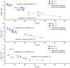 |
Fig. 12 Rotational diagrams for the vibrationally excited states of vinyl cyanide ν11 = 1, ν15 = 1, and ν11 = 2 as a function of rotational energy (upper level energy corrected from the vibrational energy of each state), which sorted by increasing vibrational energy from top to bottom. |
4.3. Rotational diagrams of CH2CHCN (g.s., ν11 = 1, 2, and ν15 = 1)
To obtain an estimate of the rotational temperature (Trot) for different velocity components, we made rotational diagrams, which related the molecular parameters with the observational ones (Eq. (1); see e.g., Goldsmith & Langer1999) for CH2CHCN in its ground state (Fig. 11) and for the lowest vibrationally excited states ν11 = 1, 2, and ν15 = 1 (Fig. 12). Assumptions, such as LTE approximation and optically thin lines (see Sect. 4.4.4), are required in this analysis. We have taken the effect of dilution of the telescope into account, which was corrected by calculation of the beam dilution factor (Demyk et al.2008, Eq. (2)):
![Mathematical equation: \begin{eqnarray} &&\ln\left(\frac{N_{\rm u}}{g_{\rm u}}\right)=\ln\left(\frac{8\pi k\nu^2W_{\rm obs}}{hc^3A_{\rm ul}g_{\rm u}}\right)=\ln\left(\frac{N}{Q_{\rm rot}}\right) - \frac{E_{\rm upp}}{kT_{\rm rot}} + \ln b, \label{eq_RD} \\[2mm] &&b=\frac{\Omega_{\rm S}}{\Omega_{\rm A}}=\frac{\theta_{\rm S}^2}{\theta_{\rm S}^2 + \theta_{\rm B}^2}, \label{eq_BDF} \end{eqnarray}](/articles/aa/full_html/2014/12/aa23622-14/aa23622-14-eq206.png) where Nu is the column density of the considered vinyl cyanide species in the upper state (cm-2), gu is the statistical weight in the upper level, Wobs (K cm s-1) is the integrated line intensity (
where Nu is the column density of the considered vinyl cyanide species in the upper state (cm-2), gu is the statistical weight in the upper level, Wobs (K cm s-1) is the integrated line intensity ( (v)dv), Aul is the Einstein A-coefficient for spontaneous emission, N (cm-2) is the total column density of the considered vinyl cyanide species, Qrot is the rotational partition function, which depends on the rotational temperature derived from the diagrams, Eupp (K) is the upper level energy, and Trot (K) is the rotational temperature. In Eq. (2), b is the beam dilution factor, ΩS and ΩA are the solid angle subtended by the source and under the main beam of the telescope, respectively, and θS and θB are the angular diameter of the source and the beam of the telescope, respectively. We note that the factor b increases the fraction Nu/gu in Eq. (1) and yields a higher column density than if it were not considered.
For the g.s., we used 117 transitions free of blending with upper level energies from 20.4 to 683.1 K with two different velocity components: one with vLSR = 4–6 km s-1 and Δv = 4–7 km s-1 and the second one with vLSR = 2–4 km s-1 and Δv = 14–20 km s-1. For the vibrationally excited states, we considered 43 (40–550 K), 24 (30–380 K), and 33 (25–370 K) transitions with line profiles that can be fitted to a single velocity component (vLSR = 4–6 km s-1 and Δv = 5–7 km s-1) for ν11 = 1, 2, and ν15 = 1, respectively.
The scatter in the rotational diagrams of CH2CHCN g.s. is mainly due to the uncertainty of fitting two Gaussian profiles to the lines with the CLASS software. Rotational diagrams of the vibrationally excited states (ν11 = 1 and ν15 = 1) are less scattered because there is only one fitted Gaussian to the line profile. For the rotational diagram of the ν11 = 2 state, the scatter is mostly due to the weakness of the observed lines for this species. We have done an effort to perform the diagrams with unblended lines; however, some degree of uncertainty could come from non-obvious blends. The individual errors of the data points are those derived by error propagation in the calculated uncertainty of ln(Nu/gu), taking only the uncertainty of the integrated intensity of each line (W) provided by CLASS and an error of 20% for the source diameter into account. The uncertainty of the final values of Trot and N has been calculated with the statistical errors given by the linear least squares fit for the slope and the intercept.
We assumed the same source diameter of 10′′ for the emitting region of the two components for the g.s. and the single component of the vibrationally excited states. In Fig. 11, the upper panel shows points in the diagram related with the wide and narrow components for the CH2CHCN g.s. We observed two tendencies in the position of the data points up to/starting from an upper state energy of ≃200 K. From the narrow component, we derived two different rotational temperatures and column densities, Trot = 125 ± 16 K and N = (1.3 ± 0.1) × 1015 cm-2, and Trot = 322 ± 57 K and N = (1.0 ± 0.2) × 1015 cm-2. Likewise, from the wide component, we have determined cold and hot temperatures of about Trot = 90 ± 14 K and Trot = 227 ± 130 K, and column densities of N = (2.9 ± 0.5) × 1015 cm-2 and N = (1.2 ± 0.9) × 1015 cm-2, respectively.
To quantify the uncertainty derived from the assumed source size, we also have performed the rotational diagram of CH2CHCN g.s. by adopting a source diameter of both 5′′ and 15′′. The main effect of changing the source size on the rotational diagram is a change in the slope and in the scatter. Table 4 shows the derived values of N and Trot by assuming different source sizes. Therefore, as expected, derived rotational temperatures depend clearly on the assumed size with a tendency to increase Trot when increasing the source diameter. The effect on the column density is less significant also due to the correction on the partition function introduced by the change in the rotational temperatures; in general, these values increased or decreased when we decreased or increased the source size, respectively (see Table 4).
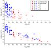 |
Fig. 13 Rotational diagram of CH2CHCN in its ground and excited states as shown as a function of rotational energy corrected from the vibrational energy in the upper panel, while the bottom panel displays the ground state followed by CH2CHCN ν11 = 1, ν15 = 1, and ν11 = 2 excited states as a function of the upper level energy. |
N and Trot from rotational diagrams of CH2CHCN g.s. which assumes different source sizes.
In Fig. 12, the panels display the rotational diagrams of the three vinyl cyanide excited states ν11 = 1, ν15 = 1, and ν11 = 2, which are sorted by the vibrational energy from top to bottom. In the x-axis we show the rotational energy which has been corrected from the vibrational energy to estimate the appropriate column density. We also observed the same tendency of the data points quoted above. The rotational temperature and the column density conditions for the ν11 = 1 were Trot = 125 ± 14 K and (2.9 ± 0.3) × 1014 cm-2, and Trot = 322 ± 104 K and N = (3 ± 1) × 1014 cm-2. For the ν15 = 1 state we determine Trot = 100 ± 20 K and N = (1.2 ± 0.2) × 1014 cm-2, and Trot = 250 ± 10 K and N = (2.4 ± 0.1) × 1014 cm-2. For the ν11 = 2 state we find that Trot = 123 ± 68 K and N = (1.0 ± 0.5) × 1014 cm-2, and Trot = 333 ± 87 K and N = (1.3 ± 0.3) × 1014 cm-2. Owing to the weakness of the emission lines of the ν11 = 3 and ν10 = 1 ⇔ (ν11 = 1,ν15 = 1) vibrational modes, we have not performed rotational diagrams for these species.
Figure 13 displays the combined rotational diagram for the ground state of CH2CHCN and ν11 = 1, ν15 = 1, and ν11 = 2 excited states. The upper panel is referred to the rotational level energies of the vinyl cyanide states, whereas the bottom panel shows the positions of the different rotational diagrams in the upper level energies when taking the vibrational energy for the excited states into account.
Owing to the large range of energies and the amount of transitions in these rotational diagrams we consider the obtained results (Trot) as a starting point in our models (see Sect. 4.4.1).
4.4. Astronomical modeling of CH2CHCN in Orion-KL
4.4.1. Analysis: the Model
From the observational line parameters derived in Sect. 4.2.1 (radial velocities and line widths), the displayed maps, and the rotational diagram results (two components, cold and hot, for each derived Gaussian fit to the line profiles), we consider that the emission of CH2CHCN species comes mainly from the four regions shown in Table 5, which are related with the hot core (those with Δv = 6–7 km s-1) and plateau/hot core (those with Δv = 20 km s-1) components. Daly et al. (2013) found that three components related with the hot core were enough to properly fit their ethyl cyanide lines. The named “Hot Core 1” and “Hot Core 3” in Daly et al. (2013) are similar to our “Hot narrow comp.” and “Cold wide comp.” of Table 5, respectively. Interferometric maps performed by Guélin et al. (2008) of ethyl and vinyl cyanide and those of Widicus Weaver & Friedel (2012) of CH3CH2CN (the latter authors affirm that in their observations CH3CH2CN, CH2CHCN, and CH3CN are cospatial) show that the emission from these species comes from different cores at the position of the hot core and IRc7. The radial velocities found in the line profiles of vinyl cyanide (between 3–5 km s-1) in this work with the cited interferometric maps could indicate that the four components of Table 5 are dominated by the emission of the hot core. For the vibrationally excited states and for the isotopologues, we found that two components (both narrow components) are sufficient to reproduce the line profiles (see Table 5). We note that we need a higher value in the line width for ν11 = 1 and ν15 = 1. This difference is probably due to a small contribution of the wide component in these lines.
Spectroscopic (Sect. 2) and observational parameters, such as radial velocity (vLSR), line width (Δv), temperature from rotational diagrams (Trot), source diameter (dsou) and offsets from the maps, were introduced in an excitation and radiative transfer code (MADEX) in order to obtain the synthetic spectrum. We have considered the telescope dilution and the position of the components with respect to the pointing position (IRc2). The LTE conditions have been assumed by owing to the lack of collisional rates for vinyl cyanide, which prevents a more detailed analysis of the emission of this molecule. Nevertheless, we expect a good approximation to the physical and chemical conditions due to the hot and dense nature of the considered components. Rotational temperatures (which coincide with the excited and kinetic temperatures in LTE conditions) have been slightly adapted from those of the rotational diagrams to obtain the best fit to the line profiles. These models allow us to obtain column density results for each species and components independently. The sources of uncertainty that were described in Tercero et al. (2010) have been considered. For the CH2CHCN g.s., ν11 = 1, and ν15 = 1 states we have adopted an uncertainty of 30%, while we have adopted a 50% uncertainty for the 13C isotopologues and the ν11 = 2, ν11 = 3, and ν10 = 1 ⇔ (ν11 = 1,ν15 = 1) states. Due to the weakness and/or high overlap with other molecular species, we only provided upper limits to the column densities of monodeuterated vinyl cyanide and the 15N isotopologue.
Physico-chemical conditions of Orion-KL from ground and excited states of CH2CHCN.
4.4.2. Column densities
The column densities that best reproduce the observations are shown in Table 5 and used for the model in Figs. 4−9 and A.2. Although the differences between the intensity of the model and that of the observations are mostly caused by blending with other molecular species, isolated vinyl cyanide lines confirm a good agreement between model and observations. We found small differences between the column density values from the model and those from the rotational diagram, likely because of the source diameters that are considered in the determination of the beam dilution for the two components.
In Figs. 4−9, 15, 16, and A.1–A.5, a model with species all already studied that have been in this survey is included (cyan line). The considered molecules and published works containing the detailed analysis for each species are as follows: OCS, CS, H2CS, HCS+, CCS, CCCS species in Tercero et al. (2010); SiO and SiS species in Tercero et al. (2011); SO and SO2 species in Esplugues et al. (2013a); HC3N and HC5N species in Esplugues et al. (2013b); CH3CN in Bell et al. (2014); CH3COOCH3 and t/g-CH3CH2OCOH in Tercero et al. (2013); CH3CH2SH, CH3SH, CH3OH, CH3CH2OH in Kolesniková et al. (2014); 13C-CH3CH2CN in Demyk et al. (2007); CH3CH215N, CH3CHDCN, and CH2DCH2CN in Margulès et al. (2009); CH3CH2CN species in Daly et al. (2013); 13C-HCOOCH3 in Carvajal et al. (2009); DCOOCH3 and HCOOCH3 in Margulès et al. (2010); 18O-HCOOCH3 in Tercero et al. (2012); HCOOCH2D in Coudert et al. (2013); 13C-HCOOCH3νt = 1, and HCOOCH3νt = 1 in Haykal et al. (2014); NH2CHO ν12 = 1 and NH2CHO in Motiyenko et al. (2007); CH2CHCN species in this work; HCOOCH3νt = 2 and CH3COOH from López et al. (in prep.).
We obtained a total column density of vinyl cyanide in the ground state of (6 ± 2) × 1015 cm-2. This value is a factor 7 higher than the value in the Orion-KL hot core of Schilke et al. (1997), who detected the vinyl cyanide g.s. in the frequency range from 325 to 360 GHz with a column density (averaged over a beam of 10′′–12′′) of 8.2 × 1014 cm-2 and a Trot of 96 K. The difference between both results is mostly due to our more detailed model of vinyl cyanide which includes four components, two of them with a source size of 5′′ (half than the beam size in Schilke et al. 1997). Sutton et al. (1995) also derived a column density of 1 × 1015 cm-2 (beam size of 13.7′′) toward the hot core position. These authors found vinyl cyanide emission toward the compact ridge position but at typical hot core velocities. Previous authors derived beam averaged column densities between 4 × 10¹³ and 2 × 1014 cm-2 (Johansson et al.1984; Blake et al.1987; Turner1991; Ziurys & McGonagle1993).
The column density of CH2CHCN ν11 = 1, (1.0 ± 0.3) × 1015 cm-2 is four times smaller than that derived for the ground state in the same components. Moreover, we derived a column density of (3 ± 2) × 1014, ≤(3 ± 2) × 1014, (5 ± 2) × 1014, and (5 ± 2) × 1014 cm-2 for the ν11 = 2, ν11 = 3, ν15 = 1, and ν10 = 1 ⇔ (ν11 = 1,ν15 = 1) states, respectively. Schilke et al. (1997) did not give column density results for the tentative detection of ν11 = 1 and ν15 = 1 bending modes. We also obtained a column density of (4 ± 2) × 1014 cm-2 for each 13C-isotopologue of vinyl cyanide.
Line opacities.
4.4.3. Isotopic abundances
It is now possible to estimate the isotopic abundance ratio of the main isotopologue (12C, 14N, 1H) with respect to 13C, 15N, and D isotopologues from the obtained column densities shown in Table 5. For estimating these ratios, we assume the same partition function for both the main and the rare isotopologues.
12C/13C: the column density ratio between the normal species and each 13C isotopologue in Orion-KL, when the associated uncertainties are considered, vary between 4–20 for the hot narrow component and between 10–43 for the cold narrow component. The solar isotopic abundance (12C/13C = 90, Anders & Grevesse1989) corresponds roughly to a factor 2–22 higher than the value obtained in Orion. The 12C/13C ratio indicates the degree of galactic chemical evolution, so the solar system value could point out earlier epoch conditions of this region (Wyckoff et al.2000; Savage et al.2002). The following previous estimates of the 12C/13C ratio in Orion-KL from observations of different molecules have been reported: 43±7 from CN (Savage et al.2002), 30–40 from HCN, HNC, OCS, H2CO, CH3OH (Blake et al.1987), 57 ± 14 from CH3OH (Persson et al.2007), 35 from methyl formate (Carvajal et al.2009, Haykal et al.2014), 45 ± 20 from CS-bearing molecules (Tercero et al.2010), 73 ± 22 from ethyl cyanide (Daly et al.2013), and ≃3–17 from cyanoacetylene in the hot core (Esplugues et al.2013b). Considering the weakness of the 13C lines, the derived ratios are compatible with a 12C/13C ratio between 30–45, which are found by other authors. Nevertheless, our results point out a possible chemical fractionation enhancement of the 13C isotopologues of vinyl cyanide. The intensity ratios derived in Sect. 4.4.4 also indicate this possibility. This ratio might be underestimated if the lines from the g.s. were optically thick. However, our model for the assumed sizes of the source yields values of τ (optical depth) that are much lower than unity (see Sect. 4.4.4). In Sgr B2(N), Müller et al. (2008) derived from their observations of CH2CHCN a 12C/13C ratio of 21 ± 6.
14N/15N: we obtained an average lower limit value for N(CH2CHC14N)/N(CH2CHC15N) of ≥33 for the two involved components. In Daly et al. (2013) (see Appendix B), we provided a 14N/15N ratio of 256 ± 128 by means of ethyl cyanide, which agree with the terrestrial value (Anders & Grevesse1989) and with the value obtained by Adande & Ziurys (2012) in the local interstellar medium. The latter authors performed an evaluation of the 14N/15N ratio across the Galaxy (toward 11 molecular clouds) through CN and HNC. They concluded that this ratio exhibits a positive gradient with increasing distance from the Galactic center (which agree with chemical evolution models where 15N has a secondary origin in novae).
D/H: for a tentative detection of mono-deuterated forms of vinyl cyanide we derived a lower limit D/H ratio of ≤0.12 (for HCDCHCN and DCHCHCN) and ≤0.09 (for CH2CDCN) for the hot narrow component, whereas we obtain ≤0.04 (for HCDCHCN and DCHCHCN) and ≤0.03 (for CH2CDCN) for the cold component. Studies of the chemistry of deuterated species in hot cores carried out by Rodgers & Millar (1996) conclude that the column density ratio D-H remains practically unaltered during a large period of time when D and H-bearing molecules are released to the gas phase from the ice mantles of dust grains. These authors indicate that the observations of deuterated molecules give insight into the processes occurring on the grain mantles by inferring the fractionation of their parent molecules. Furthermore, the fractionation also helps us to trace the physical and chemical conditions of the region (Roueff et al.2005). Values of this ratio were given by Margulès et al. (2010) from observations of deuterated methyl formate at obtained N(DCOOH3/HCOOCH3) = 0.04 for the hot core; Tercero et al. (2010) estimated an abundance ratio of N(HDCS)/N(H2CS) being 0.05 ± 0.02, which is also for the hot core component. Neil et al. (2013) provided a N(HDCO)/N(H2CO) ratio in the hot core of ≤0.005. Pardo et al. (2001b) derived a value between 0.004–0.01 in the plateau by means of N(HDO)/N(H2O). Persson et al. (2007) also for N(HDO)/N(H2O) derived 0.005, 0.001, and 0.03 for the large velocity plateau, the hot core, and the compact ridge, respectively, and Schilke et al. (1992) provided the DCN/HCN column density ratio of 0.001 for the hot core region.
4.4.4. Line opacity
The MADEX code gives us the line opacity for each transition for the physical components assumed in Table 5. Table 6 shows the opacities for the four cloud components shown in Table 5, which are obtained by varying the source diameter and the column density (the last in order to obtain a good fit between the synthetic spectra and the observations). When we decreased the source diameter, we have to increase the column densities to properly fit the observations and, therefore, the opacities of the lines increment. The extreme case, where the hot and cold cloud components have diameters of 2′′ and 5′′, respectively, allow us to obtain the maximum total opacity of ≃0.26 (sum of the opacity of all cloud components) for the 300,30–290,29 transition at 275 588 MHz. This value corresponds with a maximum correction of about 3–5% for our column density results. Column densities have to rise a factor 4 to obtain a total opacity of ≃0.95, which implies a large mismatch (a factor ≃3–4 in the line intensity) between model and observations.
Figure 14 shows the 12C/13C ratios of the observed line intensities for a given transition against its upper level energy and its frequency. As for the rotational diagrams, unblended lines have been used for deriving these ratios. We observe that most of these ratios are between 15 and 25, and we do not observe a clear decline of this ratio with either the increasing of upper state energy or the increasing of the frequency. In case of optically thick lines, we should expect these large opacities for lines at the end of the 1.3 mm window (240–280 GHz) where the upper state energies are above 150 K even for transitions of Ka = 0,1. Figure 14 suggests that the CH2CHCN g.s. lines have τ< 1. Nevertheless, if the bulk of the emission comes from a very small region (<1′′), opacities will be larger than 1.
From Fig. 14 we can estimate the average intensity ratios for each 13C isotopologue being 20 ± 6, 18 ± 5, and 19 ± 6 for 12C/13C1, 12C/13C2, and 12C/13C3, respectively. These results with the 12C/13C column density ratio derived in Sect. 4.4.3 suggests possible chemical fractionation enhancement of the 13C isotopologues of vinyl cyanide.
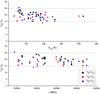 |
Fig. 14 12C/13C ratios of the observed line intensities for a given transition as a function of the upper level energy (top panel) and the frequency (bottom panel). |
4.4.5. Vibrational temperatures
We can estimate the vibrational temperature between the different vibrational modes of the vinyl cyanide according to 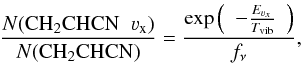 (3)where νx identifies the vibrational mode, Eνx is the energy of the corresponding vibrational state (328.5, 478.6, 657.8, 806.4/ 809.9, and 987.9 K for ν11 = 1, ν15 = 1, ν11 = 2, ν10 = 1 ⇔ (ν11 = 1,ν15 = 1), and ν11 = 3, respectively), Tvib is the vibrational temperature, fν is the vibrational partition function, N(CH2CHCN νx) is the column density of the vibrational state, and N(CH2CHCN) is the total column density of vinyl cyanide. Considering the relation N(CH2CHCN) = Ng.s. × fν and assuming the same partition function for these species in the ground and in the vibrationally excited states, we only need the energy of each vibrational state and the calculated column density to derive the vibrational temperatures. The vibrational temperature (Tvib) is given as a lower limit, since the vibrationally excited gas emitting region may not coincide with that of the ground state.
From the column density results, the Tvib in the hot narrow component for each vibrationally excited level were ≃268 ± 80 K, ≃246 ± 74 K, ≃265 ± 132 K, ≃402 ± 201 K, and ≃385 ± 192 K for ν11 = 1, ν15 = 1, ν11 = 2, ν10 = 1 ⇔ (ν11 = 1,ν15 = 1), and ν11 = 3, respectively. In the same way, the Tvib in the cold narrow component for each vibrationally excited level were ≃237 ± 71 K, ≃208 ± 62 K, ≃220 ± 110 K, ≃324 ± 162 K, and ≃330 ± 165 K for ν11 = 1, ν15 = 1, ν11 = 2, ν10 = 1 ⇔ (ν11 = 1,ν15 = 1), and ν11 = 3, respectively. The average vibrational temperature for ν11 = 1, 2, and ν15 = 1 from both narrow components was 252 ± 76 K, 242 ± 121 K, and 227 ± 68 K, respectively. In the case of ν10 = 1 ⇔ (ν11 = 1,ν15 = 1) and ν11 = 3, the derived Tvib is larger than the Trot in the hot narrow component (320 K), which could suggest an inner and hotter region for the emission of these vibrationally excited states of vinyl cyanide. Moreover, a tendency to increase the vibrational temperature with the vibrational energy of the considered state is observed. Vibrational transitions imply ro-vibrational states that may be excited by dust IR photons or collisions with the most abundant molecules in the cloud. Nevertheless, collisional rates are needed to evaluate the excitation mechanisms. The observed differences between Trot and Tvib indicate either a far-IR pumping of the highly excited vibrational levels or the presence of a strong temperature gradient toward the inner regions. Some internal heating might be reflected in temperature and density gradients due to processes such as, for example, star formation.
4.5. Detection of isocyanide species
We searched for the isocyanide counterparts of vinyl, ethyl, and methyl cyanide, cyanoacetylene, and cyanamide in our line survey. In this section, we report the first detection toward Orion-KL of methyl isocyanide, and a tentative detection of vinyl isocyanide. The first to sixth columns of Table 7 show the cyanide and isocyanide molecules studied in Orion-KL, their column density values in the components where we assumed emission from the isocyanides, the column density ratio between the cyanide and its isocyanide counterpart, the same ratio obtained by previous authors in Sgr B2 and TMC-1 sources, and the difference of the bond energies between the -CN and -NC isomers.
Column densities of the isocyanide species and N(-CN)/N(-NC) ratios.
 |
Fig. 15 Observed lines from Orion-KL (histogram spectra) and model (thin red curves) of vinyl isocyanide in its ground state. The cyan line corresponds to the model of the molecules we have already studied in this survey (see text Sect. 4.4.2) including the CH2CHCN species. We consider the detection as tentative. A vLSR of 5 km s-1 is assumed. |
Vinyl isocyanide (CH2CHNC) is an isomer of the unsaturated hydrocarbon vinyl cyanide. The structure differences between the vinyl cyanide and isocyanide are due to the CNC and CCN linear bonds and their energies, where CCN displays shorter bond distances. The bonding energy difference between vinyl cyanide and isocyanide is 8658 cm-1 (24.8 kcal mol-1) (Remijan et al.2005) with the cyanide isomer being more stable than the isocyanide. We have tentatively detected vinyl isocyanide in our line survey (Fig. 15) with 28 unblended lines and 26 partially blended lines from a total of 96 detectable lines. This detection is just above the confusion limit. In Table A.14 we show spectroscopic and observational parameters of detected lines of vinyl isocyanide. Rotational constants were derived fitting all experimental data from Bolton et al. (1970), Yamada & Winnewisser (1975), and Bestmann & Dreizler (1982); the dipole moments were from Bolton et al. (1970). For modeling this molecule, we assume the same physical conditions as those found for the vinyl cyanide species (where we consider both narrow components). We derived a column density of ≤(3 ± 2) × 1014 cm-2 (hot narrow component) and ≤(5 ± 3) × 1013 cm-2 (cold narrow component). We estimate a N(CH2CHNC)/N(CH2CHCN) ratio of ≤0.10 ± 0.05, while Remijan et al. (2005) derived a ratio of about ≤0.005 toward Sgr B2 with an upper limit for the vinyl isocyanide column density of ≤1.1 × 1013 cm-2.
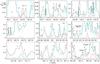 |
Fig. 16 Observed lines from Orion-KL (histogram spectra) and model (thin red curves) of methyl isocyanide in its ground state. The cyan line corresponds to the model of the molecules we have already studied in this survey (see text Sect. 4.4.2) including the CH2CHCN species. A vLSR of 5 km s-1 is assumed. |
Methyl cyanide (CH3CN) is a symmetric rotor molecule whose internal rotor leads to two components of symmetry A and E. The column densities of the ground state obtained for both A and E sub-states using an LVG model were derived by Bell et al. (2014) in Orion-KL. They separately fitted different series of K-ladders transitions (J = 6–5, J = 12–11, J = 13–12, J = 14–13). We averaged the model results for these four series at the IRc2 position deriving a column density of 3.1 × 1016 cm-2 and a kinetic temperature of ≃265 K. The CH3CN molecule has a metastable isomer named methyl isocyanide (CH3NC) that has been found in dense interstellar clouds (Sgr B2) by Cernicharo et al. (1988) and Remijan et al. (2005). The bonding energy difference between methyl cyanide and isocyanide is 9486 cm-1 (27.1 kcal mol-1) (Remijan et al.2005). We observed methyl isocyanide in Orion-KL for the first time (Fig. 16). For modeling the weak lines of methyl isocyanide we assume a hot core component (T = 265 K, dsou = 10′′, offset = 3′′, vLSR = 5 km s-1, Δv = 5 km s-1) that is consistent with those derived by Bell et al. (2014). Rotational constants were derived from a fit to the data reported by Bauer & Bogey (1970), Pracna et al. (2011). The constants HJ, LJ, and LJKKK have been fixed to the values derived by Pracna et al. (2011). The constants A and DK were from Pliva et al. (1995). Dipole moment was that of Gripp et al. (2000). We derived a column density of (3.0 ± 0.9)×1013 cm-2 for each A and E symmetry substates. We determined a N(CH3NC)/N(CH3CN) ratio of 0.002 which is a factor 15–25 lower than the value obtained by Cernicharo et al. (1988) toward Sgr B2. DeFrees et al. (1985) by means of chemical models predicted this ratio in dark clouds in the range of 0.1–0.4.
Ethyl cyanide (CH3CH2CN) is a heavy asymmetric rotor with a rich spectrum. In our previous paper (Daly et al.2013), three cloud components were modeled in LTE conditions to determine the column density9 of this molecule. We obtained a total column density of (7 ± 2) × 1016 cm-2 for this species.
The bonding energy difference between ethyl cyanide and isocyanide is 8697 cm-1 (24.9 kcal mol-1) (Remijan et al.2005). The spectroscopic parameters used for ethyl isocyanide (CH3CH2NC) were obtained from recent measurements in Lille up to 1 THz by Margulès et al. (in prep.). For CH3CH2NC we provide an upper limit to its column density of (2 ± 1) × 1014 cm-2. Then, we derived a N(CH3CH2NC)/N(CH3CH2CN) ratio of 0.003. This value is 100 times lower than the upper limit value obtained by Remijan et al. (2005) toward Sgr B2 of ≤0.3.
We observe that the upper limit for the CH2CHNC column density is 5 times higher than the value of methyl isocyanide and holds a similar order of magnitude relationship with the upper limit column density of the tentatively detected ethyl isocyanide.
Cyanoacetylene (HCCCN) is a linear molecule with a simple spectrum. Its lines emerge from diverse parts of the cloud (Esplugues et al.2013b), although mainly from the hot core. The model of the HCCCN lines was set up using LVG conditions. The authors determined a total column density of (3.5 ± 0.8) × 1015 cm-2.
Isocyanoacetylene (HCCNC) is a stable isomer of cyanoacetylene and has an energy barrier of 6614 cm-1 (18.9 kcal mol-1). Owing to high overlap problems in our data, we only found one line of HCCNC free of blending at 99 354.2 MHz. To obtain an upper limit for its column density we assumed the same physical components as those of Esplugues et al. (2013b). Spectroscopic parameters were derived by fitting the lines reported by Guarnieri et al. (1992); the dipole moment was taken from Gripp et al. (2000). We obtained an upper limit to the HCCNC column density of ≤(3 ± 1) × 1013 cm-2. We estimated an upper limit for the N(HCCNC)/N(HCCCN) ratio of ≤0.008. The molecule HCCNC was observed for the first time toward TMC-1 (three rotational lines in the frequency range 40–90 GHz) by Kawaguchi et al. (1992a). They obtained a N(HCCNC)/N(HCCCN) ratio in the range 0.02–0.05 in that dark cloud, which is around 2–6 times higher than our upper limit. Ohishi & Kaifu (1998) provided an upper limit value of ≤0.001 also in TMC-1. This molecule has also been detected in the envelope of the carbon star IRC+10216 by Gensheimer (1997).
The other carbene-type isomer of HCCCN is 3-imino-1, 2-propadienylidene (HNCCC) that was predicted to have a relative energy of about 17744.6 cm-1 with respect to HCCCN (Kawaguchi et al.1992b). We provided a tentative detection of this isomer in our survey (Fig. A.3). Its column density, (3 ± 1) × 1013 cm-2, has been obtained by assuming the same cloud components as those of Esplugues et al. (2013b). Spectroscopic parameters were derived from a fit to lines reported by Kawaguchi et al. (1992b) and Hirahara et al. (1993), and three lines observed in IRC+10216 with an accuracy of 0.3 MHz. The dipole moment was determined from Botschwina et al. (1992). We derived a N(HNCCC)/N(HCCCN) upper limit ratio of 0.008. Kawaguchi et al. (1992a) obtained a N(HNCCC)/N(HCCCN) ratio in the range 0.002–0.006 in TMC-1.
After the detection of cyanamide (NH2CN) by Turner et al. (1975), Cummins et al. (1986), and Belloche et al. (2013) in Sgr B2, we report a tentative detection of cyanamide (NH2CN) in Orion-KL (see Fig. A.4). Frequencies, energies, and line intensities for O+-NH2CN and O−-NH2CN were those published in the JPL catalog (based on the works of Read et al.1986 and Birk1988). We estimated a column density ≤(3 ± 1) × 1013 cm-2 (O++O−) by assuming that its lines are coming only from one component (hot core) at 200 K (vLSR = 5 km s-1, Δv = 5 km s-1, dsou = 10′′, offset = 2′′). NH2CN has an isomer differing only in the CN group, so that, the isomerization energy between the cyanamide and isocyanamide (NH2NC) is 18 537 cm-1 (Vincent & Dykstra1980). In this work, we also provided only an upper limit column density of isocyanamide (O++O−) being ≤(5 ± 1) × 1013 cm-2. Spectroscopic parameters were derived fitting the rotational lines reported by Schäfer et al. (1981). the dipole moment was determined by Ichikawa et al. (1982) from ab-initio calculations.
In Table 7, we give values of interconversion energies between cyanide and isocyanide molecules. These interconversion barriers are high, and under astronomical environments, such as the hot cores, it is unlikely that the isocyanide isomers are produced by rearrangement of the corresponding cyanide species. Remijan et al. (2005), proposed that non-thermal processes (such as shocks or enhanced UV flux in the surrounding medium) may be the primary route to the formation of interstellar isocyanides by the conversion of the cyanide to its isocyanide counterpart. Nevertheless, other formation routes have to be explored to explain their presence in environments dominated by thermal processes. Dissociative recombination reactions on the gas phase probably lead to the formation of the cyanide or isocyanide molecules. Depending on the structure of the protonated hydrocarbon and the branching ratios of the dissociative recombination pathway, the molecule H2C3N+ might produce cyanoacetylene and isocyanoacetylene, and similarly, the molecule C2H4N+ could yield methyl cyanide and methyl isocyanide (Green & Herbst1979). DeFrees et al. (1985) found that the calculated ratio of the formation of the protonated precursor ions (CH3CNH+ and CH3NCH+) agrees with the detection of CH3NC in dark clouds (Irvine & Schloerb1984). In the same way, the recombination reaction of the molecule C2H6N+ could give ethyl isocyanide (Bouchoux et al.1992). Once the isocyanides are formed, they remain as metastable species due to the high barrier quoted above supporting the possible existence of isolated isocyanides (Vincent & Dykstra1980). On the other hand, a recent experimental study of the interaction of the diatomic radical CN and the π-system C2H4 confirms that the possible pathway to CH2CHNC becomes negligible even at temperatures as high as 1500 K (Balucani et al.2000; Leonori et al.2012). Since the cyanide molecules are strongly related to the dust chemistry (Blake et al.1987; Charnley et al.1992; Caselli et al.1993; Rodgers & Charnley2001; Garrod et al.2008; Belloche et al.2013), we also can infer a probable origin for the isocyanides from reactions on grain mantles.
5. Discussion
5.1. Abundances and column density ratios between the cyanide species
Table 8 shows the ground state abundances in the hot core (or hot core + plateau) component of the studied species in this work and the column density ratios between vinyl cyanide and other cyanide molecules. Results provided by different authors in Orion-KL, the well-studied star forming region Sgr B2, the star forming complex G34.3+0.2 (hot core), and the dark molecular cloud TMC-1 are also given in this table.
For Orion-KL, our study covers a wide frequency range allowing detailed modeling of the molecular emission. Moreover, the molecular abundances obtained from other authors, which are shown in Table 8, are often obtained with different telescopes and different assumptions on the size and physical conditions of Orion-KL. For this reason, these abundances are given in Table 8 for comparison purposes, but we focus on the results obtained in this work that have been derived from a common set of assumptions, sizes, and physical conditions for Orion-KL.
To estimate molecular abundances for the cyanide and isocyanide species, we assume that the column density of H2 (NH2) is 4.2 × 1023 cm-2 for the hot core, 2.1 × 1023 cm-2 for the plateau, and 7.5 × 1022 cm-2 for the compact ridge and for the extended ridge, as derived by Tercero et al. (2010).
The total abundance for the CH2CHCN ground state, as derived from all the components (hot core + mix hot core-plateau) (see Table 5), was X(NCH2CHCN/NH2) = (2.0 ± 0.6) × 10-8. By means of the derived vibrational temperatures, we can estimate the vibrational partition function that follows the Eq. (4) for a Boltzmann distribution in both narrow components (1.7 and 1.5 for hot and cold narrow components, respectively) and correct the ground state column density to the total one (see Sect. 4.4.5). Considering these results for the vibrational partition function, we obtained XCH2CHCN ≃ (3.1 ± 0.9) × 10-8. 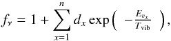 (4)where dx is the degeneracy of the vibrational mode x and the low Tvib leads to fν ≃ 1.
Column density ratios and molecular abundances.
Assuming the column density values of CH3CN of Bell et al. (2014), the abundance for CH3CN ground state in the hot core component was ≃(1.0 ± 0.3) × 10-7. To estimate the correction of the column density of CH3CN from excited vibrational states, we have derived the column density of this molecule in its ν8 = 1 lower energy state (525.2 K) and found a N(CH3CN,ν8 = 1) ≃ 1.4 × 1015 cm-2 and Tvib ≃ 159 K (considering only the hot core and plateau components). Hence, the vibrational partition function is ~1.04 and XTotal ≃ Xground for methyl cyanide.
For ethyl cyanide we use the column density results of Daly et al. (2013) (see Appendix B). We determine the X(NCH3CH2CN/NH2) ratio being (1.8 ± 0.5) × 10-7 for the ground state. Assuming the vibrational temperatures obtained in Daly et al. (2013) ≃160 ± 50 K, ≃185 ± 55 K, and ≃195 ± 95 K for ν13/ν21 (Eu = 306.3/315.4 K), ν20 (Eu = 531.2 K), and ν12 (Eu = 763.4 K), respectively, the estimated vibrational partition function is 1.4, so we derived an abundance ratio X ≃ (2.5 ± 0.8) × 10-7 for ethyl cyanide.
Esplugues et al. (2013b) derived an abundance of 7.3 × 10⁻⁹ for HC3N (hot core + plateau) in the ground state.
Assuming a mean vibrational temperature of 360 K in the hot core that is calculated by these authors, the vibrational partition function from ν5 (Eu = 954.48), ν6 (Eu = 718.13), ν7 = 1 (Eu = 320.45), and ν7 = 2 (Eu = 642.67) is ~2.6 for the hot core components. Applying this correction in the hot core, we obtained a total abundance of XHC3N ≃ 1.3 × 10⁻⁸ (hot core + plateau).
For NH2CN, we determine a molecular abundance X(NNH2CN/NH2) of ≤(7 ± 2) × 10-11.
The column density ratio between the unsaturated hydrocarbon CH2CHCN and other -CN bearing molecules, such as CH3CH2CN, CH3CN, HC3N, and NH2CN, N(CH2CHCN)/ N(X-CN), could be used to track a possible different evolutionary state described by different chemical models and to provide inputs for the chemical modeling of the cloud.
We obtain an abundance ratio N(CH2CHCN)/N(X-CN)<1 for the saturated cyanide molecules (CH3CH2CN and CH3CN); these ratios related with methyl and ethyl cyanide obtained by different authors are lower (in general) in Orion-KL than in the galactic center (Sgr B2). We also note that the relative abundance of CH3CH2CN with respect to vinyl cyanide in Orion is twice as much as in the hot core G34.3+0.2. In contrast, in the dark cloud TMC-1 vinyl cyanide is more abundant than the saturated -CN hydrocarbons.
The relative abundance between CH2CHCN and HC3N follows an opposite tendency than that of methyl and ethyl cyanide: HC3N is less abundant than CH2CHCN in Orion-KL and Sgr B2, whereas HC3N is at least two orders of magnitude more abundant than CH2CHCN in TMC-1. Nevertheless, we want to remark that we only address the hot core (or hot core + plateau) abundances in our work in Table 8. For vinyl and ethyl cyanide and cyanamide, these abundances correspond with the total abundance in the ground state in Orion-KL. However, cyanoacetylene appears in all the Orion-KL components, so its total abundance is higher than that of vinyl cyanide when we consider the whole Orion-KL region covered by our observations.
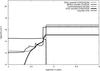 |
Fig. 17 Time evolution of the column densities of CH2CHCN, CH3CN, CH3CH2CN, HC3N, and CN for a hot core chemical model. |
Finally, we find an lower limit of 286 for X(CH2CHCN)/ X(NH2CN).
The formation routes of the cyanide molecules in several environments have been extensively discussed by different authors. As ethyl cyanide was mainly detected in hot core regions (Johansson et al.1984; Sutton et al.1985; Blake et al.1987), the grain surface production (by hydrogenation of HC3N) seemed to be the main formation mechanisms for this molecule (Blake et al.1987; Charnley et al.1992; Caselli et al.1993). On the other hand, vinyl cyanide has been detected in the dark could TMC-1 (Matthews & Sears1983) and in hot cores (where appeared correlated with ethyl cyanide emission), indicating that gas phase production was also important for forming these species. Chemical models of Charnley et al. (1992) and Caselli et al. (1993) in hot cores predicted that CH2CHCN forms in gas phase reactions involving CH3CH2CN. Caselli et al. (1993) derived a relation between the abundance ratio X(CH2CHCN)/X(CH3CH2CN) and the evolutionary stage of the core. This ratio has been used by several authors as a chemical clock to estimate the cloud age (Fontani et al.2008; Müller et al.2008). Belloche et al. (2009) performed a detailed analysis of the cyanide species detected in Sgr B2, including chemical models based on that of Garrod et al. (2008). Considering the observed relative abundances between these species, they conclude that the main formation mechanism for alkyl cyanides is probably the sequential addition of CH2 or CH3 radicals to CN, CH2CN, and C2H4CN on the grain surfaces. Formation of methyl cyanide is dominated by reactions on the grains by addition of CH3 and CN radicals, but it may also be formed by gas-phase processes after the evaporation of HCN. Vinyl cyanide is predominantly formed in the gas-phase through the reaction of CN with C2H4. Then CH2CHCN accretes onto the grains by being a potential precursor, with HC3N of ethyl cyanide and n-propyl cyanide. After the evaporation of the ice mantles, vinyl cyanide is efficiently formed again in the gas phase.
5.2. Chemical model
We have investigated the observed column densities of CH2CHCN, CH3CN, CH3CH2CN, HCCCN, and CN using a time and depth dependent gas-grain chemical model, UCL_CHEM. UCL_CHEM is a two-phase model, which follows the collapse of a prestellar core (Phase I), followed by the warming and evaporation of grain mantles (Phase II). In Phase II, we increase the dust and gas temperature up to 300 K to simulate the presence of a nearby infrared source in the core. For the hot core component, we model both a 10 M⊙ and 15 M⊙ star with a final density of 107 cm -3. During the collapse, atoms and molecules collide with and freeze onto grain surfaces. The depletion efficiency is determined by the fraction of the gas-phase material that is frozen on to the grains, which is dependent on the density, the sticking coefficient and other properties of the species and grains (see Rawlings et al.1992). In our modeling, we have explored the uncertainty in grain properties and sticking coefficients by varying the depletion percentage. Initial atomic abundances are taken from Sofia & Meyer (2001), as in Viti et al. (2004). Gas-phase reaction rate coefficients are taken from the UMIST database of Woodall et al. (2007), however, some have been updated with those from the KIDA database (Wakelam2009). We also include some simple grain-surface reactions (mainly hydrogenation) as in Viti et al. (2004). While COMs (complex organic molecules) may also form via surface reactions involving heavier (than hydrogen) species (e.g. Garrod et al.2008), the mobility of most heavy species on grains has not been experimentally investigated; hence, for this qualitative analysis, we chose to adopt a simpler model where only the most efficient surface reactions occur. In this way we can give a lower limit to the formation of COMs which may be augmented by more complex reactions should they occur. In Phase I, non-thermal desorption is considered as in Roberts et al. (2007).
Within our grid of models, we find that models where we simulate a 10 M⊙ star and 100% of CO frozen onto grain surfaces which most accurately reproduce the observed column densities of CH2CHCN, CH3CN, and CH3CH2CN. Figure 17 shows the column density as a function of time during phase II for this model. The column density produced by the model for HCCCN is an order of magnitude higher than the observed value. While our models simulate both gas phase and grain surface reactions for all of these species, the grain surface reactions are essential to reproduce the observed column densities. We therefore conclude that we are missing some grain surface destruction routes for HCCCN, and, consequently, overproduced this species in our models. Moreover, the deep decreased of the CN abundance when CH3CH2CN appears is observationally confirmed by the lack of the hot core component in the CN lines even at the HIFI frequencies (Crockett et al.2014). For details of the same surface chemistry approach, see Viti et al. (2004) and Bell et al. (2014).
5.3. Further issues for CH2CHCN
Further observations of telescopes with higher sensitivity and spatial resolution, such as Atacama Large Millimeter/submillimeter Array (ALMA), could provide additional detections of other vibrationally excited states above 600 cm-1, such as the outstanding states in the 3ν11/2ν15/ν14 triad of states near 680 cm-1 for which the spectroscopy is presently reported. In this study, we found that the ν11 = 3 (987.9 K or 686.6 cm-1) vibrational mode was near the detection limit, so we could not reliably address other vibrational components of the 3ν11/2ν15/ν14 triad. We also note that Belloche et al. (2013) have recently detected the combination state ν15 = ν11 = 1 (809.9 K) but has not yet reported detection of the ν10 = 1 (806.4 K) state toward Sgr B2(N). On the other hand, the ν15 = 2 (960.2 K) excited state detected by these authors might be detected only at the limit in our study.
In the present work, we extended the laboratory coverage of the rotational spectrum of vinyl cyanide and the analysis of its vibrationally excited states to provide ample basis for detection of transitions from further excited vibrational states at even higher vibrational energies. The laboratory basis for detecting states up to as high as ν9 = 1 (1250 K) is now available. On the other hand, as implied by Fig. 1 and results for 4ν11 = 4, considerable spectroscopic analysis is required for satisfactory understanding of states above ν9 = 1.
6. Summary
Vinyl cyanide is one of the most abundant molecules in Orion-KL and a possible precursor of alanine. This study of the vinyl cyanide species improves the knowledge of the physical and chemical conditions of this high-mass star forming region. We have performed an identification of the ground state of CH2CHCN and of its vibrationally excited states (up to 988 K) in the Orion-KL Nebula thanks to a new spectroscopic laboratory analysis by using Stark modulation and frequency-modulated spectrometers. Our results are based on rotational diagrams, integrated-frequency maps, and Gaussian fits to optimize the physical and chemical parameters that simulate the best synthetic spectrum of CH2CHCN (using MADEX), which fit the observation conditions of the Orion-KL region in an accurate way. We have found N(CH2CHCN) ≃(6 ± 2) × 1015 cm-2 from four cloud components of hot core/plateau nature (320-90 K). A total abundance of (3.1 ± 0.9) × 10-8 for vinyl cyanide is provided in this work. We have detected the CH2CHCN ν11 = 2, 3 vibrational modes for the first time in Orion-KL and the CH2CHCN ν10 = 1 ⇔ (ν11 = 1,ν15 = 1) excited state for the first time in the space. We have seen that these species with those of the three monosubstituted 13C and the 15N isotopologues and the tentative detection of the three monodeuterated species of vinyl cyanide contribute with more than 1100 observed lines in the 80–280 GHz domain covered by the Orion line survey. We highlight the importance for spectroscopic catalogs to introduce vibrationally excited species in the astronomical detections.
The column density ratios between the vinyl cyanide g.s. and the vibrationally excited states have been used to obtain temperatures at which the vibrational modes are excited and to correct the ground column density from the vibrational partition function. The high vibrational temperature (Tvib>Trot) for the states ν10 = 1 ⇔ (ν11 = 1,ν15 = 1) and ν11 = 3 suggests a temperature gradient toward the inner regions of the hot core. To infer the population mechanism of the vibrationally excited states (collisions and/or infrared radiation), collisional rates are needed.
Owing to the importance of isomerism for understanding a more precise way in forming interstellar molecules, we have included the study of ethyl isocyanide, methyl isocyanide, isocyanoacetylene, 3-imino-1, 2-propadienylidene, and isocyanamide in our work. We have provided the detection of methyl isocyanide for the first time in Orion-KL and tentative detections for the rest.
Finally, we have investigated the studied column densities of CH2CHCN, CH3CN, CH3CH2CN, and HCCCN using a time dependent gas-grain chemical model (UCL_CHEM) which reproduce the observed column densities for these molecules reasonably well, although it overestimates that for HCCCN. This is probably due to the efficiency for its formation on the grains being too high: a detailed investigation of the formation and destruction route for this species in chemical models is beyond the scope of this work. More quantitative models ought to be able to reproduce this molecule by investigating the efficiency of the formation of HCCCN on the grains.
Frisch, M. J.; Trucks, G. W.; Schlegel, et al., Gaussian 09, Revision B.01; Gaussian: Wallingford, CT, 2010.
Stanton, J. F., Gauss, J.; Harding, M. E. et al., CFOUR, a quantum chemical quantum package with integrated packages MOLECULE (Almlof, J.; Taylor, P. R.) and ECP routines (Mitin, A. V.; van Wüllen, C.), http://www.cfour.de
The data of the IRAM-30 m line survey of Orion-KL are available is ASCII format on request to B. Tercero and J. Cernicharo and will be available on the IRAM web page.
Cernicharo private catalogs, CDMS (Müller et al.2001, 2005), and JPL (Pickett et al.1998).
We found a typographical error that is twice the difference in the column density of the hot core component 1 for the ground and excited states in our previous paper (Daly et al.2013) hence the isotopic abundance has to be modified. We have attached the tables of column densities and that of isotopic abundance for CH3CH2CN in Appendix B.
Acknowledgments
We thank the anonymous referee who provided comments that improved this manuscript. We thank INTA-CSIC, and the Spanish MINECO and Junta de Castilla y León for funding support from grants the CONSOLIDER program “ASTROMOL” CSD2009-00038, AYA2009-07304, AYA2012-32032, CTQ2010-19008 and VA175U13. C.B. thanks also the Spanish MINECO for the FPI grant (BES-2011-047695). The IFPAN authors acknowledge a grant from the Polish National Science Centre, decision number DEC/2011/02/A/ST2/00298. Portions of this research were carried out at the Jet Propulsion Laboratory, California Institute of technology, under contract with the National Aeronautics and Space Administration.
References
- Adande, G. R., & Ziurys, L. M. 2012, ApJ, 744, 194 [NASA ADS] [CrossRef] [Google Scholar]
- Anderson, R. J., & Gwinn, W. D. 1968, J. Chem. Phys., 49, 39, 88 [CrossRef] [Google Scholar]
- Agúndez, M., Cernicharo, J., Pardo, J. R., et al. 2008, Astron. Space Sci., 313, 229 [NASA ADS] [CrossRef] [Google Scholar]
- Anders, E., & Grevesse, N. 1989, Geochim. Cosmochim. Acta, 53, 197 [Google Scholar]
- Balucani, N., Asvany, O., Huang, L. C. L., et al. 2000, ApJ, 545, 892 [NASA ADS] [CrossRef] [Google Scholar]
- Baskakov, O. I., Dyubko, S. F., Ilyushin, V. V., et al. 1996, J. Mol. Spectr., 179, 94 [NASA ADS] [CrossRef] [Google Scholar]
- Bauer, A., & Bogey, M. 1970, C. R. Acad. Sci. Paris, 271B, 892 [Google Scholar]
- Bell, T., Cernicharo, J., Viti, S., et al. 2014, A&A, 564, A114 [NASA ADS] [CrossRef] [EDP Sciences] [Google Scholar]
- Belloche, A., Garrod, T. D., Müller, H. S. P., et al. 2009, A&A, 499, 215 [NASA ADS] [CrossRef] [EDP Sciences] [Google Scholar]
- Belloche, A., Müller, H. S. P., Menten, K. M., Schilke, P., & Comito, C. 2013, A&A, 559, A47 [NASA ADS] [CrossRef] [EDP Sciences] [Google Scholar]
- Bera, P. P., Lee, T. J., & Schaefer, H. F. 2009, J. Chem. Phys., 131, 074303 [NASA ADS] [CrossRef] [Google Scholar]
- Bestmann, G., & Dreizler, H. 1982, Z. Naturforsch, 37a, 58 [Google Scholar]
- Betz, A. L. 1981, ApJ, 244, L103 [NASA ADS] [CrossRef] [Google Scholar]
- Beuther, H., & Nissen, H. D. 2008, ApJ, 679, L121 [NASA ADS] [CrossRef] [Google Scholar]
- Birk, H. 1988, Ph.D. Thesis, Justus Liebig-Universit Giessen, Germany [Google Scholar]
- Blake, G. A., Sutton, E. C., Masson, C. R., & Philips, T. G. 1987, ApJ, 315, 621 [NASA ADS] [CrossRef] [Google Scholar]
- Blake, G. A., Mundy, L. G., Carlstrom, J., et al. 1996, ApJ, 472, L49 [NASA ADS] [CrossRef] [Google Scholar]
- Bolton, K., Owen, N. L., & Sheridan, J. 1970, Spectrochim. Acta, 26, 909 [CrossRef] [Google Scholar]
- Botschwina, P., Horn, M., Seeger, S., & Flgge, J. 1993, Chem. Phys. Lett., 195, 4, 427 [Google Scholar]
- Bouchoux, G., Nguyen, M. T., & Longevialle, P. 1992, J. Am. Chem. Soc., 114, 10000 [CrossRef] [Google Scholar]
- Capone, L. A., Prasad, S. S., Huntress, W. T., et al. 1981, Nature, 293, 45 [NASA ADS] [CrossRef] [Google Scholar]
- Carvajal, M., Margulés, L., Tercero, B., et al. 2009, A&A, 500, 1109 [NASA ADS] [CrossRef] [EDP Sciences] [Google Scholar]
- Caselli, P. 2005, Ap&SS Library, 324, 47 [Google Scholar]
- Caselli, P., Hasegawa, T. I., & Herbst, E. 1993, ApJ, 408, 548 [NASA ADS] [CrossRef] [Google Scholar]
- Cazzoli, G., & Kisiel, Z. 1988, J. Mol. Spectr., 130, 303 [Google Scholar]
- Cernicharo, J. 1985, Internal IRAM report (Granada: IRAM) [Google Scholar]
- Cernicharo, J. 2012, in ECLA-2011: Proc. of the European Conference on Laboratory Astrophysics, EAS Pub. Ser. 2012, eds. C. Stehl, C. Joblin, & L. d’Hendecourt (Cambridge: Cambridge Univ. Press), 58, 251 [Google Scholar]
- Cernicharo, J., Kahane, C., Guelin, M., & Gomez-Gonzalez, J. 1988, A&A, 189, L1 [NASA ADS] [Google Scholar]
- Cernicharo, J., Tercero, B. A., Fuente, A., et al. 2013, ApJ, 771, L10 [NASA ADS] [CrossRef] [Google Scholar]
- Charnley, S. B., Tielens, A. G. G. M., & Millar, T. J. 1992, ApJ, 399, L71 [NASA ADS] [CrossRef] [Google Scholar]
- Cole, A. R. H., & Green, A. A. 1973, J. Mol. Spectr., 48, 246 [NASA ADS] [CrossRef] [Google Scholar]
- Colmont, J. M., Wlodarczak, G., Priem, D., et al. 1997, J. Mol. Spectr., 181, 330 [Google Scholar]
- Costain, C. C., & Stoicheff, B. P. 1959, J. Chem. Phys., 1959, 30, 777 [Google Scholar]
- Coudert, L. H., Drouin, B. J., Tercero, B., et al. 2013, ApJ, 779, 119 [NASA ADS] [CrossRef] [Google Scholar]
- Crockett, N. R., Bergin, E. A., Neill, J. L., et al. 2014, ApJ, 787, 2 [NASA ADS] [CrossRef] [Google Scholar]
- Cummins, S. E., Linke, R. A., & Thaddeus, P. 1986, ApJSS, 60, 819 [NASA ADS] [CrossRef] [Google Scholar]
- Daly, A. M., Bermúdez, C., López, A., et al. 768, 81, ApJ, 2013 [Google Scholar]
- Demaison, J., Cosléou, J., Bocquet, R., & Lesarri, A. G. 1994, J. Mol. Spectr., 167, 400 [NASA ADS] [CrossRef] [Google Scholar]
- Demyk, K., Mäder, H., Tercero, B., et al. 2007, A&A, 466, 255 [NASA ADS] [CrossRef] [EDP Sciences] [Google Scholar]
- Demyk, K., Wlodarczak, G., & Carvajal, M. 2008, A&A, 489, 589 [NASA ADS] [CrossRef] [EDP Sciences] [Google Scholar]
- DeFrees, D. J., McLean, A. D., & Herbst, E. 1985, ApJ, 293, 236 [NASA ADS] [CrossRef] [Google Scholar]
- Ervasti, H. K., Jobst, K. J., Gerbaux, P., et al. 2009, Chem. Phys. Lett., 482, 211 [NASA ADS] [CrossRef] [Google Scholar]
- Esplugues, G. B., Tercero, B., Cernicharo, J., et al. 2013a, A&A, 556, A143 [NASA ADS] [CrossRef] [EDP Sciences] [Google Scholar]
- Esplugues, G. B., Cernicharo, J., Viti, S., et al. 2013b, A&A, 559, A51 [NASA ADS] [CrossRef] [EDP Sciences] [Google Scholar]
- Fliege, E., & Dreizler, H. 1985, Z. Naturforsch., 40a, 43 [Google Scholar]
- Fontani, F., Caselli, P., Bourke, T. L., Cesaroni, R., & Brand, J. 2008, A&A, 477, L45 [NASA ADS] [CrossRef] [EDP Sciences] [Google Scholar]
- Gardner, F. F., & Winnewisser, G. 1975, ApJ, 195, L127 [Google Scholar]
- Garrod, R. T., Weaver, S. L. W., & Herbst, E. 2008, ApJ, 682, 283 [NASA ADS] [CrossRef] [Google Scholar]
- Gensheimer, P. D. 1997, Ap&SS, 251, 199 [NASA ADS] [CrossRef] [Google Scholar]
- Gerry, M. C. L., & Winnewiser, G. 1973, J. Mol. Spectr., 48, 1 [NASA ADS] [CrossRef] [Google Scholar]
- Golsmith, P. F., & Langer, W. D. 1999, ApJ, 517, 209 [NASA ADS] [CrossRef] [Google Scholar]
- Green, S., & Herbst, E. 1979, ApJ, 229, 121 [Google Scholar]
- Gripp, J., Guarnieri, A., Stahl, W., & Lentz, D. 2000, J. Mol. Struc. 526, 81 [Google Scholar]
- Guarnieri, A., Hinze, R., Krüger, M., et al. 1992, J. Mol. Spectr., 156, 1, 39 [CrossRef] [Google Scholar]
- Guélin, M., Brouillet, N., Cernicharo, J., Combes, F., & Wooten, A. 2008, Ap&SS, 313, 45 [NASA ADS] [CrossRef] [Google Scholar]
- Halverson, F., Stamm, R. F., & Whalen, J. J. 1948, J. Chem. Phys., 16, 808 [NASA ADS] [CrossRef] [Google Scholar]
- Haykal, I., Carvajal, M., Tercero, B., et al. 2014, A&A, 568, A58 [NASA ADS] [CrossRef] [EDP Sciences] [Google Scholar]
- Heise, H. M., Lutz, H., & Dreizler, H. 1974, Z. Naturforsch., 29, 1345 [Google Scholar]
- Hirahara, Y., Ohshima, Y., & Endo, Y. 1993, ApJ, 403, L83 [NASA ADS] [CrossRef] [Google Scholar]
- Hirota, T., Bushimata, T., Choi, Y. K., et al. 2007, PASJ, 59, 897 [NASA ADS] [CrossRef] [Google Scholar]
- Ichikawa, K., Hamada, Y., Sugawara, Y., et al. 1982, Chem. Phys., 72, 301 [NASA ADS] [CrossRef] [Google Scholar]
- Irvine, W. M., & Schloerb, F. P. 1984, ApJ, 282, 516 [Google Scholar]
- Irvine, W. M., Friberg, P., Hjalmarson, A., et al. 1988, ApJ, 334, L107 [NASA ADS] [CrossRef] [Google Scholar]
- Johansson, L. B. E., Andersson, C., Elldèr, J., et al. 1984, A&A, 130, 227 [NASA ADS] [PubMed] [Google Scholar]
- Johnson, D. R., Lovas, F. J., Guélin, M., & Thaddeus, P. 1977, ApJ, 218, 370 [NASA ADS] [CrossRef] [Google Scholar]
- Kawaguchi, K., Ohishi, M., & Ishikawa, S.-I. 1992a, ApJ, 386, L51 [NASA ADS] [CrossRef] [Google Scholar]
- Kawaguchi, K., Takano, S., Ohishi, M., et al. 1992b, ApJ, 396, L49 [NASA ADS] [CrossRef] [Google Scholar]
- Khlifi, M., Nollet, M., Paillous, P., et al. 1999, J. Mol. Spectr., 194, 206 [NASA ADS] [CrossRef] [Google Scholar]
- Kim, M. K., Hirota, T., Honma, M., et al. 2008, PASJ, 60, 991 [NASA ADS] [CrossRef] [Google Scholar]
- Kisiel, Z. 2001, in Spectroscopy from Space, eds. J., Demaison, et al. (Dordrecht: Kluwer Academic Publishers), 91 [Google Scholar]
- Kisiel, Z., Pszczolkowski, L., Medvedev, I. R., et al. 2005, J. Mol. Spectr., 233, 231 [NASA ADS] [CrossRef] [Google Scholar]
- Kisiel, Z., Pszczolkowski, L., Drouin, B. J., et al. 2009a, J. Mol. Spectr., 258, 26 [Google Scholar]
- Kisiel, Z., Bialkowska-Jaworska, E., Butler, R. A. H, et al. 2009b, J. Mol. Spectr., 254, 78 [NASA ADS] [CrossRef] [Google Scholar]
- Kisiel, Z., Pszczolkowski, L., Drouin, B. J., et al. 2011, talk MH09, 66th International Symp. on Molecular Spectroscopy, Columbus, Ohio, USA [Google Scholar]
- Kisiel, Z., Pszczolkowski, L., Drouin, B. J., et al. 2012, J. Mol. Spectr., 280, 134 [Google Scholar]
- Kolesniková, L., Tercero, B., Cernicharo, J., et al. 2014, ApJ, 784, L7 [NASA ADS] [CrossRef] [Google Scholar]
- Krasnicki, A., & Kisiel, Z. 2011, J. Mol. Spectr., 270, 83 [NASA ADS] [CrossRef] [Google Scholar]
- Krasnicki, A., Kisiel, Z., Drouin, B. J., & Pearson, J. C. 2011, J. Mol. Struct., 1006, 20 [NASA ADS] [CrossRef] [Google Scholar]
- Krüger, M., & Dreizler, H. 1992, Z. Naturforsch., 47a, 1067 [Google Scholar]
- Leonori, F., Petrucci, R., Wang, X., Casavecchia, P., & Balucani, N. 2012, Chem. Phys. Lett., 553, 1 [NASA ADS] [CrossRef] [Google Scholar]
- Margulès, L., Motiyenko, R. A., Demyk, K., et al. 2009, A&A, 493, 565 [NASA ADS] [CrossRef] [EDP Sciences] [Google Scholar]
- Margulès, L., Huet, T. R., Demaison, J., et al. 2010, ApJ, 714, 1120 [NASA ADS] [CrossRef] [Google Scholar]
- Mathews, H. E., & Sears, T. J. 1983, ApJ, 267, L53 [Google Scholar]
- Martinez, Jr., O., Lattanzi, V., Thorwirth, S., & McCarthy, M. C. 2013, J. Chem. Phys., 138, 094316 [NASA ADS] [CrossRef] [Google Scholar]
- Menten, K. M., Reid, M. J., Forbrich, J., & Brunthaler, A. 2007, A&A, 474, 515 [NASA ADS] [CrossRef] [EDP Sciences] [Google Scholar]
- Mehringer, D. M., & Snyder, L. 1996, ApJ, 471, 897 [NASA ADS] [CrossRef] [Google Scholar]
- Minh, Y. C., & Irvine, W. M. 1991, Ap&SS, 175, 165 [Google Scholar]
- Morris, M., Turner, B. E., Palmer, P., & Zuckerman, B. 1976, ApJ, 205, 82 [NASA ADS] [CrossRef] [Google Scholar]
- Motiyenko, R. A., Tercero, B., Cernicharo, J., & Margulés, L. 2012, A&A, 548, A71 [NASA ADS] [CrossRef] [EDP Sciences] [Google Scholar]
- Müller, H. S. P., Thorwirth, S., Roth, D. A., & Winnewisser, G. 2001, A&A, 370, L49 [NASA ADS] [CrossRef] [EDP Sciences] [Google Scholar]
- Müller, H. S. P., Schlöder, F., Stutzki, J., & Winnewisser, G. 2005, J. Mol. Struct., 742, 215 [NASA ADS] [CrossRef] [Google Scholar]
- Müller, H. S. P., Belloche, A., Menten, Comito, C., & Shilke, P. 2008, J. Mol. Spectr., 251, 319 [NASA ADS] [CrossRef] [Google Scholar]
- Neil, J. L., Crockett, N. R., Bergin, E. A., Pearson, J. C., & Li-Hong, Xu 2013, ApJ, 777, 85 [NASA ADS] [CrossRef] [Google Scholar]
- Nummelin, A., & Bergman, P. 1999, A&A, 341, L59 [NASA ADS] [Google Scholar]
- Nummelin, A., Bergman, P., Hjalmarson, Å, et al. 2000, ApJSS, 128, 213 [NASA ADS] [CrossRef] [Google Scholar]
- Occhiogrosso, A., Viti, S., & Balucani, N. 2013, MNRAS, 432, 3423 [NASA ADS] [CrossRef] [Google Scholar]
- Ohisi, M., & Kaifu, N. 1998, J. Chem. Soc. Faraday Discuss., 109, 205 [Google Scholar]
- Pardo, J. R., Cernicharo, J., & Serabyn, E. 2001a, IEEE Tras. Antennas and Propagation, 49, 1683 [NASA ADS] [CrossRef] [Google Scholar]
- Pardo, J. R., Cernicharo, J., Herpin, F., Kawamura, J., et al. 2001b, ApJ, 562, 799 [NASA ADS] [CrossRef] [Google Scholar]
- Persson, C. M., Olofsson, A. O. H., Koning, N., et al. 2007, A&A, 476, 2, 807 [NASA ADS] [CrossRef] [EDP Sciences] [Google Scholar]
- Petrie, S. A. H. 1991, Ph.D. Thesis, University of Canterbury, New Zealand (ir.canterbury.ac.nz) [Google Scholar]
- Pickett, H. M. 1991, J. Mol. Spectr., 148, 371 [NASA ADS] [CrossRef] [Google Scholar]
- Pickett, H. M., Poynter, R. L., Cohen, E. A., et al. 1998, J. Quant. Spectr. Rad. Transf., 60, 883 [NASA ADS] [CrossRef] [Google Scholar]
- Pliva, J., Le, L. D., Johns, J. W. C., Lu, Z., & Bernheim, R. A. 1995, J. Mol. Spectr., 173, 2, 423 [Google Scholar]
- Pracna, P., Urban, J., Votava, O., et al. 2011, J. Phys. Chem. A., 115, 1063 [CrossRef] [Google Scholar]
- Rawlings, J. M. C., Hartquist, T. W., Menten, K. M., & Williams, D. A. 1992, MNRAS, 255, 471 [NASA ADS] [CrossRef] [Google Scholar]
- Read, W. G., Cohen, E. A., & Pickett, H. M. 1986, J. Mol. Spectr., 115, 316 [Google Scholar]
- Remijan, A. J., Hollis, J. M., Lovas, F. J., Plusquellic, D. F., & Jewell, P. R. 2005, ApJ, 632, 333 [NASA ADS] [CrossRef] [Google Scholar]
- Roberts, J. F., Rawlings, J. M. C., Viti, S., & Williams, D. A. 2007, MNRAS, 382, 733 [NASA ADS] [CrossRef] [Google Scholar]
- Rodgers, S. D., & Charnley, S. B. 2001, ApJ, 546, 324 [Google Scholar]
- Rodgers, S. D., & Millar, T. J. 1996, MNRAS, 280, 1046 [NASA ADS] [CrossRef] [Google Scholar]
- Roueff, E., Lis, D. C., vander Tak, F. F. S., Gerin, M., & Goldsmith, P. F. 2005, A&A, 438, 585 [NASA ADS] [CrossRef] [EDP Sciences] [Google Scholar]
- Sandstrom, K. M., Peek, J. E. G., Bower, G. C., et al. 2007, ApJ, 667, 1161 [NASA ADS] [CrossRef] [Google Scholar]
- Savage, C., Apponi, A. J., Ziurys, L. M., & Wyckoff, S. 2002, ApJ, 578, 211 [NASA ADS] [CrossRef] [Google Scholar]
- Schäfer, E., & Winnewisser, M. 1982, Ber. Bunsenges. Phys. Chem., 86, 780 [CrossRef] [Google Scholar]
- Schäfer, E., Winnewisser, M., & Christiansen, J. J. 1981, Chem. Phys. Lett., 81, 380 [NASA ADS] [CrossRef] [Google Scholar]
- Schilke, P., Walmsley, C. M., Pineau Des Forets, G., et al. 1992, A&A, 256, 595 [NASA ADS] [Google Scholar]
- Schilke, P., Groesbeck, T. D., Blake, G. A., & Philips, T. G. 1997, ApJSS, 108, 301 [NASA ADS] [CrossRef] [Google Scholar]
- Sofia, U. J., & Meyer, D. M. 2001, ApJ, 554, L221 [NASA ADS] [CrossRef] [Google Scholar]
- Stolze, M., & Sutter, D. H. 1985, Z. Naturforsch. Teil A, 40a, 998 [Google Scholar]
- Sutton, E. C., Blake, G. A., Masson, C. R., & Phillips, T. G. 1985, A&A, 58, 341 [Google Scholar]
- Sutton, E. C., Peng, R., Danchi, W. C., et al. 1995, ApJSS, 97, 455 [NASA ADS] [CrossRef] [Google Scholar]
- Tercero, B. 2012, Thesis UCM, Spain [Google Scholar]
- Tercero, B., Cernicharo, J., Pardo, J. R., & Goicoechea, J. R. 2010, A&A, 517, A96 [NASA ADS] [CrossRef] [EDP Sciences] [Google Scholar]
- Tercero, B., Vincent, L., Cernicharo, J., Viti, S., & Marcelino, N. 2011, A&A, 528, A26 [NASA ADS] [CrossRef] [EDP Sciences] [Google Scholar]
- Tercero, B., Margulès, L., Carvajal, M., et al. 2012, A&A, 538, 119 [Google Scholar]
- Tercero, B., Kleiner, I., Cernicharo, J., et al. 2013, ApJ, 770, L13 [Google Scholar]
- Tielens, A. G. G. M. 2005, The Physics and Chemistry of the Interstellar Medium (Cambridge University Press) [Google Scholar]
- Turner, B. E. 1991, ApJSS, 76, 617 [CrossRef] [Google Scholar]
- Turner, B. E., Kyslyakov, A. G., Liszt, H. S., & Kaifu, N. 1975, ApJ, 201, L149 [Google Scholar]
- Vigren, E., Hamberg, M., Zhaunerchyk, V., et al. 2009, ApJ, 695, 317 [NASA ADS] [CrossRef] [Google Scholar]
- Vincet, M. A., & Dykstra, C. E. 1980, J. Chem. Phys., 73, 3838 [NASA ADS] [CrossRef] [Google Scholar]
- Viti, S., Collings, M. P., Dever, J. W., McCoustra, M. R. S., & Williams, D. A., 2004, MNRAS, 354, 1141 [NASA ADS] [CrossRef] [Google Scholar]
- Wakelam, V. 2009, BAAS, 41, 665 [Google Scholar]
- Widicus Weaver, S. L., & Friedel, D. N. 2012, ApJS, 201, 16 [NASA ADS] [CrossRef] [Google Scholar]
- Wilcox, W. S., Goldstein, J. H., & Simmons, J. W. 1954, J. Chem. Phys., 22, 516 [NASA ADS] [CrossRef] [Google Scholar]
- Woodall, J., Agúndez, M., MarkwickKemper, A. J., & Millar, T. J. 2007, A&A, 466, 1197 [NASA ADS] [CrossRef] [EDP Sciences] [Google Scholar]
- Wyckoff, S., Kleine, M., Peterson, B. A., Wehinger, P. A., & Ziurys, L. M. 2000, ApJ, 535, 991 [NASA ADS] [CrossRef] [Google Scholar]
- Yamada, K., & Winnewisser, M. 1975, Z. Naturforsch, A, 30, 672 [Google Scholar]
- Ziurys, L. M., & McGonagle, D. 1993, ApJSS, 89, 155 [NASA ADS] [CrossRef] [Google Scholar]
Appendix A
Spectroscopic constants in the diagonal blocks of the Hamiltonian for the 2ν15 ⇔ ν14 ⇔ 3ν11 triad of vibrational states in vinyl cyanide compared with those for the ground state.
Spectroscopic constants in the off-diagonal blocks of the Hamiltonian for the ν10 ⇔ ν11ν15 and ν11ν10 ⇔ 2ν11ν15 dyads of vibrational states in vinyl cyanide.
Spectroscopic constants in the off-diagonal blocks of the Hamiltonian for the 2ν15 ⇔ ν14 ⇔ 3ν11 triad of vibrational states in vinyl cyanide.
Spectroscopic constants in the effective rotational Hamiltonian for the ν9 and 4ν11 excited vibrational states of vinyl cyanide.
Vibrational changes in rotational constantsa for the studied excited vibrational states in vinyl cyanide.
 |
Fig. A.1 Observed lines from Orion-KL (histogram spectra) and model (thin red curves) of CH2CHCN of ν11 = 3. The cyan line corresponds to the model of the molecules we have already studied in this survey (see text Sect. 4.4.2), including the CH2CHCN species. A vLSR of 5 km s-1 is assumed. |
 |
Fig. A.2 Observed lines from Orion-KL (histogram spectra) and model (thin red curves) of deuterated isotopes for CH2CHCN in the ground state. The subindex of Di (i = 1, 2, 3) correspond to the position of the isotope in the molecule (D1CD2CD3CN). The cyan line corresponds to the model of the molecules we have already studied in this survey (see text Sect. 4.4.2), including the CH2CHCN species. A vLSR of 5 km s-1 is assumed. |
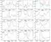 |
Fig. A.3 Observed lines from Orion-KL (histogram spectra) and model (thin red curves) of 3-imino-1,2-propadienyllidene in its ground state. The cyan line corresponds to the model of the molecules we have already studied in this survey (see text Sect. 4.4.2), including the CH2CHCN species. A vLSR of 5 km s-1 is assumed. |
 |
Fig. A.4 Observed lines from Orion-KL (histogram spectra) and model (thin red curves) of cyanamide in its ground state. The cyan line corresponds to the model of the molecules we have already studied in this survey (see text Sect. 4.4.2), including the CH2CHCN species. A vLSR of 5 km s-1 is assumed. |
 |
Fig. A.5 Observed lines from Orion-KL (histogram spectra) and model (thin red and blue curves) of isocyanamide in its ground state. The cyan line corresponds to the model of the molecules we have already studied in this survey (see text Sect. 4.4.2), including the CH2CHCN species. A vLSR of 5 km s-1 is assumed. |
Detected lines of CH2CHCN g.s.
Detected b-type lines of CH2CHCN g.s.
Detected lines of CH2CHCN ν11 = 1.
Detected lines of CH2CHCN ν11 = 2.
Detected lines of CH2CHCN ν11 = 3.
Detected lines of CH2CHCN ν15 = 1.
Detected lines of CH2CHCN ν10 = 1 ⇔ (ν11 = 1,ν15 = 1).
Detected lines of 13C1, 13C2, and 13C3 isotopologues of CH2CHCN.
Detected lines of vinyl isocyanide (CH2CHNC).
Appendix B: Typographical error in Daly et al. (2013)
Physico-chemical conditions of Orion-KL from CH3CH2CN.
Isotopic abundances for CH3CH2CN in the Orion-KL region.
All Tables
Spectroscopic data sets for excited vibrational states of CH2CHCN acquired in this work.
Spectroscopic constants in the diagonal blocks of the Hamiltonian for the ν10 ⇔ ν11ν15 and the ν11ν10 ⇔ 2ν11ν15 dyads of vibrational states in vinyl cyanide compared with those for the ground state.
N and Trot from rotational diagrams of CH2CHCN g.s. which assumes different source sizes.
Physico-chemical conditions of Orion-KL from ground and excited states of CH2CHCN.
Spectroscopic constants in the diagonal blocks of the Hamiltonian for the 2ν15 ⇔ ν14 ⇔ 3ν11 triad of vibrational states in vinyl cyanide compared with those for the ground state.
Spectroscopic constants in the off-diagonal blocks of the Hamiltonian for the ν10 ⇔ ν11ν15 and ν11ν10 ⇔ 2ν11ν15 dyads of vibrational states in vinyl cyanide.
Spectroscopic constants in the off-diagonal blocks of the Hamiltonian for the 2ν15 ⇔ ν14 ⇔ 3ν11 triad of vibrational states in vinyl cyanide.
Spectroscopic constants in the effective rotational Hamiltonian for the ν9 and 4ν11 excited vibrational states of vinyl cyanide.
Vibrational changes in rotational constantsa for the studied excited vibrational states in vinyl cyanide.
All Figures
|
Fig. 1 All vibrational levels of vinyl cyanide up to 1000 cm-1. The levels in red are those for which rotational transitions have been analyzed in this work. The boxes identify sets of levels treated by means of coupled fits accounting for interstate perturbations. |
| In the text | |
|
Fig. 2 Room-temperature laboratory spectrum of vinyl cyanide in the region of the 413 − 312 rotational transition recorded with a Stark modulation spectrometer. All marked lines are for the 413 − 312 transition in a given vibrational or isotopic species and display a characteristic pattern of negative lobes due to the non-zero field cycle of Stark modulation. Dotted lines connect vibrational states analyzed as perturbing polyads, red denotes vibrational states analyzed in the present work, and asterisks identify states detected presently in Orion-KL. It can be seen that laboratory analysis is now available for excited vibrational state transitions that are comparable in room-temperature intensity to those for 13C isotopologues in terrestrial natural abundance. |
| In the text | |
|
Fig. 3 Effect of vibration-rotation perturbations on frequencies of the strongest rotational transitions in the ν10 ⇔ ν11ν15 dyad of vibrational states. The plotted quantities are scaled frequency differences relative to the same transitions in the ground state. Continuous lines are predictions from the final fit; circles mark assigned lines and traces in each panel have added vertical shifts to improve clarity. |
| In the text | |
|
Fig. 4 Observed lines from Orion-KL (histogram spectra) and model (thin red curves) of vinyl cyanide in the ground state. The cyan line corresponds to the model of the molecules we have already studied in this survey (see text Sect. 4.4.2), including the CH2CHCN species. A vLSR of 5 km s-1 is assumed. |
| In the text | |
|
Fig. 5 Observed lines from Orion-KL (histogram spectra) and model (thin red curves) of CH2CHCN of ν11 = 1. The cyan line corresponds to the model of the molecules we have already studied in this survey (see text Sect. 4.4.2), including the CH2CHCN species. A vLSR of 5 km s-1 is assumed. |
| In the text | |
|
Fig. 6 Observed lines from Orion-KL (histogram spectra) and model (thin red curves) for the ν15 = 1 vibrational state of CH2CHCN. The cyan line corresponds to the model of the molecules we have already studied in this survey (see text Sect. 4.4.2), including the CH2CHCN species. A vLSR of 5 km s-1 is assumed. |
| In the text | |
|
Fig. 7 Observed lines from Orion-KL (histogram spectra) and model (thin red curves) for the ν11 = 2 vibrational state of CH2CHCN. The cyan line corresponds to the model of the molecules we have already studied in this survey (see text Sect. 4.4.2), including the CH2CHCN species. A vLSR of 5 km s-1 is assumed. |
| In the text | |
|
Fig. 8 Observed lines from Orion-KL (histogram spectra) and model (thin red curves) for combined vibrationally excited states of CH2CHCN in the ν10 = 1 ⇔ (ν11 = 1, ν15 = 1) dyad. The cyan line corresponds to the model of the molecules we have already studied in this survey (see text Sect. 4.4.2), including the CH2CHCN species. A vLSR of 5 km s-1 is assumed. |
| In the text | |
|
Fig. 9 Observed lines from Orion-KL (histogram spectra) and model (thin red curves) of 13C isotopes for CH2CHCN in the ground state. The subindex in 13Ci (i = 1, 2, 3) corresponds to the position of the isotope in the molecule (i1CH |
| In the text | |
|
Fig. 10 Integrated intensity maps for 6 ground state transitions of vinyl cyanide. From line 1 (top row) to 6 (bottom row): 121,12–111,11 (110 839.98 MHz, 36.8 K), 240,24–230,23 (221 766.03 MHz, 134.5 K), 242,23–232,22 (226 256.88 MHz, 144.8 K), 261,26–251,25 (238 726.808 MHz, 157.4 K), 262,25–252,24 (244 857.47 MHz, 167.9 K), and 2410,15–2310,14 and 2410,14–2310,13 (228017.34 MHz, 352.0 K) at different velocity ranges (indicated in the top of each column). Three boxes have been blanked because the emission at these velocities was blended with that from other well known species. For each box axis are in units of arcseconds (Δα, Δδ). Color logarithm scale is the integrated intensity ( |
| In the text | |
|
Fig. 11 Rotational diagram of CH2CHCN in its ground state. The upper panel displays the two components derived from the line profiles. The middle panel shows two linear fits to the narrow component points; these linear regressions yield temperatures and column densities of Trot = 125 ± 16 K and N = (1.3 ± 0.1) × 1015 cm-2 (Qrot = 7.06 × 10³), and Trot = 322 ± 57 K and N = (1.0 ± 0.2) × 1015 cm-2 (Qrot = 2.92 × 10⁴). Likewise, the bottom panel shows another two linear fits to the points corresponding to the wide component. The results of these fits are rotational temperatures of Trot = 90 ± 14 K and Trot = 227 ± 130 K, and column densities of (2.9 ± 0.5) × 1015 cm-2 (Qrot = 4.31 × 10³) and (1.2 ± 0.9)×1015 cm-2 (Qrot = 1.73 × 10⁴), respectively. |
| In the text | |
|
Fig. 12 Rotational diagrams for the vibrationally excited states of vinyl cyanide ν11 = 1, ν15 = 1, and ν11 = 2 as a function of rotational energy (upper level energy corrected from the vibrational energy of each state), which sorted by increasing vibrational energy from top to bottom. |
| In the text | |
|
Fig. 13 Rotational diagram of CH2CHCN in its ground and excited states as shown as a function of rotational energy corrected from the vibrational energy in the upper panel, while the bottom panel displays the ground state followed by CH2CHCN ν11 = 1, ν15 = 1, and ν11 = 2 excited states as a function of the upper level energy. |
| In the text | |
|
Fig. 14 12C/13C ratios of the observed line intensities for a given transition as a function of the upper level energy (top panel) and the frequency (bottom panel). |
| In the text | |
|
Fig. 15 Observed lines from Orion-KL (histogram spectra) and model (thin red curves) of vinyl isocyanide in its ground state. The cyan line corresponds to the model of the molecules we have already studied in this survey (see text Sect. 4.4.2) including the CH2CHCN species. We consider the detection as tentative. A vLSR of 5 km s-1 is assumed. |
| In the text | |
|
Fig. 16 Observed lines from Orion-KL (histogram spectra) and model (thin red curves) of methyl isocyanide in its ground state. The cyan line corresponds to the model of the molecules we have already studied in this survey (see text Sect. 4.4.2) including the CH2CHCN species. A vLSR of 5 km s-1 is assumed. |
| In the text | |
|
Fig. 17 Time evolution of the column densities of CH2CHCN, CH3CN, CH3CH2CN, HC3N, and CN for a hot core chemical model. |
| In the text | |
|
Fig. A.1 Observed lines from Orion-KL (histogram spectra) and model (thin red curves) of CH2CHCN of ν11 = 3. The cyan line corresponds to the model of the molecules we have already studied in this survey (see text Sect. 4.4.2), including the CH2CHCN species. A vLSR of 5 km s-1 is assumed. |
| In the text | |
|
Fig. A.2 Observed lines from Orion-KL (histogram spectra) and model (thin red curves) of deuterated isotopes for CH2CHCN in the ground state. The subindex of Di (i = 1, 2, 3) correspond to the position of the isotope in the molecule (D1CD2CD3CN). The cyan line corresponds to the model of the molecules we have already studied in this survey (see text Sect. 4.4.2), including the CH2CHCN species. A vLSR of 5 km s-1 is assumed. |
| In the text | |
|
Fig. A.3 Observed lines from Orion-KL (histogram spectra) and model (thin red curves) of 3-imino-1,2-propadienyllidene in its ground state. The cyan line corresponds to the model of the molecules we have already studied in this survey (see text Sect. 4.4.2), including the CH2CHCN species. A vLSR of 5 km s-1 is assumed. |
| In the text | |
|
Fig. A.4 Observed lines from Orion-KL (histogram spectra) and model (thin red curves) of cyanamide in its ground state. The cyan line corresponds to the model of the molecules we have already studied in this survey (see text Sect. 4.4.2), including the CH2CHCN species. A vLSR of 5 km s-1 is assumed. |
| In the text | |
|
Fig. A.5 Observed lines from Orion-KL (histogram spectra) and model (thin red and blue curves) of isocyanamide in its ground state. The cyan line corresponds to the model of the molecules we have already studied in this survey (see text Sect. 4.4.2), including the CH2CHCN species. A vLSR of 5 km s-1 is assumed. |
| In the text | |
Current usage metrics show cumulative count of Article Views (full-text article views including HTML views, PDF and ePub downloads, according to the available data) and Abstracts Views on Vision4Press platform.
Data correspond to usage on the plateform after 2015. The current usage metrics is available 48-96 hours after online publication and is updated daily on week days.
Initial download of the metrics may take a while.