| Issue |
A&A
Volume 563, March 2014
|
|
|---|---|---|
| Article Number | A87 | |
| Number of page(s) | 20 | |
| Section | Interstellar and circumstellar matter | |
| DOI | https://doi.org/10.1051/0004-6361/201323092 | |
| Published online | 14 March 2014 | |
Relating jet structure to photometric variability: the Herbig Ae star HD 163296⋆,⋆⋆
1 Astronomical Institute “Anton Pannekoek”, University of Amsterdam, Science Park 904, 1098 XH Amsterdam, The Netherlands
e-mail: lucas.ellerbroek@gmail.com
2 Institut de Planétologie et d’Astrophysique de Grenoble, 414 rue de la Piscine, 38400 St.-Martin d’ Hères, France
3 INAF − Osservatorio Astrofisico di Arcetri, Largo Enrico Fermi 5, 50125 Florence, Italy
4 CNRS/Universidad de Chile, Laboratoire Franco-Chilien d’Astronomie (LFCA), UMI 3386 Santiago, Chile
5 LERMA, Observatoire de Paris, UMR 8112 du CNRS, 61 Av. de l’Observatoire, 75014 Paris, France
6 Department of Physics, University of Cincinnati, Cincinnati OH 45221, USA
7 Space Science Institute, 4750 Walnut Street, Boulder, CO 80303, USA
8 Space Telescope Science Institute, 3700 San Martin Drive, Baltimore, MD 21218, USA
9 Instituut voor Sterrenkunde, KU Leuven, Celestijnenlaan 200B, 3001 Leuven, Belgium
10 Leiden Observatory, Leiden University, PO Box 9513, 2300 RA Leiden, The Netherlands
11 Lunar and Planetary Laboratory, The University of Arizona, Tucson, AZ 85721, USA
12 Department of Physics and Astronomy, Clemson University, Clemson, SC 29634-0978, USA
13 Eureka Scientific, Inc., Oakland, CA 94602, USA
14 Exoplanets and Stellar Astrophysics Laboratory, Code 667, Goddard Space Flight Center, Greenbelt, MD 20771, USA
15 Crimean Astrophysical Observatory, Scientific Research institute, 98409 Crimea, Nauchny, Ukraine
16 The Aerospace Corporation, Los Angeles, CA 90009, USA
17 Thule Scientific, Topanga, CA 90290, USA
18 Associated Universities for Research in Astronomy, Inc., 1212 New York Ave. NW, Washington, DC 20005, USA
19 Department of Astronomy, University of Washington, Seattle, WA 98105, USA
20 Department of Physics, Miami University, Oxford, OH 45056, USA
21 Department of Management Science and Engineering, Stanford University, Stanford, CA 94305, USA
22 American Association of Variable Star Observers, 49 Bay State Road, Cambridge, MA 02138, USA
23 Harvard-Smithsonian Center for Astrophysics, 60 Garden Street, Cambridge, MA 02138, USA
Received: 20 November 2013
Accepted: 15 January 2014
Herbig Ae/Be stars are intermediate-mass pre-main sequence stars surrounded by circumstellar dust disks. Some are observed to produce jets, whose appearance as a sequence of shock fronts (knots) suggests a past episodic outflow variability. This “jet fossil record” can be used to reconstruct the outflow history. We present the first optical to near-infrared (NIR) spectra of the jet from the Herbig Ae star HD 163296, obtained with VLT/X-shooter. We determine the physical conditions in the knots and also their kinematic “launch epochs”. Knots are formed simultaneously on either side of the disk, with a regular interval of ~16 yr. The velocity dispersion versus jet velocity and the energy input are comparable between both lobes. However, the mass-loss rate, velocity,and shock conditions are asymmetric. We find Ṁjet/Ṁacc ~ 0.01−0.1, which is consistent with magneto-centrifugal jet launching models. No evidence of any dust is found in the high-velocity jet, suggesting a launch region within the sublimation radius (<0.5 au). The jet inclination measured from proper motions and radial velocities confirms that it is perpendicular to the disk. A tentative relation is found between the structure of the jet and the photometric variability of the central source. Episodes of NIR brightening were previously detected and attributed to a dusty disk wind. We report for the first time significant optical fadings lasting from a few days up to a year, coinciding with the NIR brightenings. These are very likely caused by dust lifted high above the disk plane, and this supports the disk wind scenario. The disk wind is launched at a larger radius than the high-velocity atomic jet, although their outflow variability may have a common origin. No significant relation between outflow and accretion variability could be established. Our findings confirm that this source undergoes periodic ejection events, which may be coupled with dust ejections above the disk plane.
Key words: stars: formation / circumstellar matter / stars: variables: T Tauri, Herbig Ae/Be / ISM: jets and outflows / Herbig-Haro objects / stars: individual: HD 163296
Based on observations performed with X-shooter (program 089.C-0874) mounted on the ESO Very Large Telescope on Cerro Paranal, Chile.
Appendix A is available in electronic form at http://www.aanda.org
© ESO, 2014
1. Introduction
Herbig Ae/Be stars (HAeBe) are intermediate-mass (2−10 M⊙) pre-main sequence stars. Like their low-mass equivalent, the classical T Tauri stars (CTTS), HAeBe stars are associated with accretion disks and, in a few cases, jets (e.g., Corcoran & Ray 1998; Grady et al. 2000, 2004). Key questions are how exactly these jets are launched and how this process relates to disk accretion (Ferreira et al. 2006; Bai & Stone 2013). In Herbig systems, the jet-disk coupling may be different than in CTTS. The relatively high stellar luminosity causes grain particles to rapidly evaporate at distances within ~1 au, creating a dust-free zone (Kama et al. 2009). Accretion is observed in HAeBe stars (e.g., Muzerolle et al. 2004; Mendigutía et al. 2011), so an inner gas disk most likely exists. Since jets are expected to originate (at least in part) in this region (Blandford & Payne 1982), they may help to improve our understanding of the coupling of accretion and outflow in the inner disk.
We may constrain the launching process by observing jet structure and motion. Jets from young stars are usually observed as a sequence of shock fronts or “knots”. These are probably the result of a variable outflow velocity (Rees 1978; Raga et al. 1990). A significant asymmetry in velocity and shock conditions is often observed between the two lobes of the jets (Hirth et al. 1994; Ray et al. 2007). By tracing the trajectories of the knots through space, we are able to reconstruct the epochs when they were formed and their (quasi-)periodic occurrence, if any (e.g., Ellerbroek et al. 2013). On-source photometric and spectroscopic observations that were made during these “launch epochs” (when available) may shed light on what happens in the disk whenever a knot is created. These observations may also clarify the origin of the asymmetry between lobes, which is observed in many jet systems. In this paper we combine time-resolved jet and disk observations and diagnostics to constrain the properties of the launch mechanism, the structure of the launch region, the origin of jet asymmetry, and the relation with disk accretion.
The Herbig Ae star HD 163296 is a promising test case for this observing strategy. Its disk has been well-studied and is associated with a jet, and a copious amount of time-resolved imaging and spectroscopic data are available. Located at a distance of 119 ± 11 pc (van Leeuwen 2007), the system does not appear to be associated with a star-forming cluster or dark cloud (Finkenzeller & Mundt 1984). Meeus et al. (2012) do find extended [C ii] emission that may originate in a background or a surrounding molecular cloud.
The bipolar jet HH 409 was discovered on coronagraphic images (and later confirmed with long-slit spectra) of the Space Telescope Imaging Spectrograph (STIS) on the Hubble Space Telescope (HST; Grady et al. 2000; Devine et al. 2000). One of the knots (A) has also been associated with X-ray emission (Swartz et al. 2005). The high-velocity gas in the jet has radial velocities of 200 − 300 km s-1. A blue-shifted molecular outflow (up to 13′′ from the source) was found in CO 2−1 and 3−2 emission with the Atacama Large Millimiter Array (ALMA) by Klaassen et al. (2013) and also recovered on Sub-Millimeter Array CO 2−1 images (C. Qi, priv. comm.). The material in the molecular outflow propagates an order of magnitude slower than the fast-moving jet, peaking at −18 km s-1 in the systemic rest frame.
The radius of the dust disk around HD 163296 is estimated at around 500 au, based on the non-detection of the red-shifted jet up to this distance (Grady et al. 2000) and the extent of the scattered light emission (Wisniewski et al. 2008). The 850 μm continuum emission is observed up to ~240 au; the outer gas disk is detected in CO lines with a Keplerian rotation profile (Rosenfeld et al. 2013; de Gregorio-Monsalvo et al. 2013).
The near-infrared (NIR) excess has a component that peaks at 3 μm and is well fitted by a blackbody of 1500 K. This suggests emission by dust at the evaporation temperature. Interferometric observations (Tannirkulam et al. 2008a; Benisty et al. 2010a) show that a major fraction of this emission originates within the theoretical dust sublimation radius (Rsub ~ 0.5 au for HD 163296, Eq. (1) in Dullemond & Monnier 2010). Also, the emission profile is smooth, i.e., does not originate in a sharply contrasted inner disk rim. HD 163296 also shows significant variations in its NIR brightness on timescales of years (Sitko et al. 2008).
A number of scenarios have been put forward to explain these observations. Hydrostatic disk models are not preferred, as the NIR emission is much stronger than predicted by hydrostatic equilibrium; also, these scenarios do not explain the photometric variability. Alternative scenarios include a dust halo (Vinković et al. 2006) and a dusty disk wind (Bans & Königl 2012). In both cases, dust would not exist within Rsub, but at larger distances and above the disk plane, making its observation within Rsub a projection effect. Vinković & Jurkić (2007) suggest that dust ejections, possibly related to jet launching, are responsible for NIR excess and variability.
The “fossil record” contained in the jet as described above may help constrain the physical properties and variability of the inner regions of the disk. In this paper we present optical to NIR spectra of the jet and central source. These were obtained with X-shooter on the ESO Very Large Telescope (VLT). We combine the spectra and archival images to reveal the outflow history of the system. We then compare this with the photometric variability of the central object. In Sect. 2 we describe the newly obtained and archival observational data. In Sect. 3 we present our analysis of the jet kinematics and physical conditions. In Sect. 4, we present a multi-band lightcurve of the central object compiled from archival and previously unpublished data. We analyze the variability and colors of the source, and estimate its historic accretion rate. In Sect. 5 we discuss the constraints put on the jet launching by our observations. We also propose a possible explanation for the source variability and comment on its relation with jet structure. We present our conclusions in Sect. 6.
Journal of the X-shooter observations.
2. Observations, data reduction and archival data
In this section we give an overview of the spectroscopic and photometric data presented in this paper. An image of the jet in [S ii] and the definition of the knots can be found in Wassell et al. (2006, W06; their Fig. 1).
2.1. VLT/X-shooter spectroscopy
Spectra of HD 163296 and its jet were obtained with VLT/X-shooter (Vernet et al. 2011), which covers the optical to NIR spectral region in three separate arms: UVB (290−590 nm), VIS (550−1010 nm), and NIR (1000−2480 nm). Table 1 lists the settings and characteristics of the observations. To observe the jet, multiple overlapping pointings of the 11′′ slit were performed. On 6 July 2012, one short on-source exposure was followed by several offsets, covering both lobes of the HH 409 jet up to 25′′. A narrow-slit deeper exposure covering the red lobe up to 40′′ was taken on 7 July 2012. Sky frames were obtained before or after every exposure to correct for telluric emission lines. Since the source is very bright, we have acquired the jet spectra by offsetting the slit with respect to the source. As a result, the inner jet region (<5′′) is not covered in the 2012 observations. On 2 and 14 July 2013, follow-up observations were carried out in two offsets up to 2′′ from the source, in order to constrain the positions of the inner knots.
The frames were reduced using the X-shooter pipeline (version 1.5.0, Modigliani et al. 2010), employing the standard steps of data reduction, i.e., bias subtraction, order extraction, flat fielding, wavelength calibration, and sky subtraction, to produce two-dimensional spectra. The wavelength calibration was verified by fitting selected OH lines in the sky spectrum, resulting in a calibration accuracy of a few km s-1. Flux-calibration was performed using spectra of the spectrophotometric standard star GD153 (a DA white dwarf). The width of the knots perpendicular to the jet axis was assumed to be narrower than the seeing, so that the slit losses were estimated from measuring the seeing FWHM from the spatial profile of a point source on the 2D frame (on the first night, HD 163296, on the second night, a telluric standard star). These estimates were refined by comparing the obtained SED to the averaged photometry (see Sect. 4.1). They were subsequently corrected for the slit widths used in the jet observations. This procedure results in an uncertainty of about 10% on the absolute flux calibration; the relative flux calibration is accurate to within 3%.
The wavelengths and velocities used throughout this paper are expressed in the systemic rest frame, for which we adopt νsys = 5.8 ± 0.2 km s-1 with respect to the Local Standard of Rest, determined by Qi et al. (2011) based on sub-mm emission lines from the outer disk. This value agrees with the observed radial velocity of photospheric absorption lines in the X-shooter spectrum of HD 163296, which give 7.2 ± 2.0 km s-1.
After reduction, the frames were merged, averaging the overlapping regions between observations. In the observations closest to the source, a reflection (“ghost spectrum”) of the central source was present at the edges of the slit. We subtracted this contribution in the following way. In a region around every emission line of interest, at every spatial row in the 2D frames, we divided the spectral profile by the on-source spectrum. We then fitted a zero-order polynomial to the residual. Finally, the original spectral profile was divided by the source spectrum multiplied by this fitted value. This results in a position−velocity diagram free of source contamination (Fig. 1). Faint, residual continuum emission is seen at + 6 − 7′′, which most likely results from a background continuum source (also visible at this location in the images of Grady et al. 2000).
2.2. Archival data
Measurements of the positions of knots A, B, and C were made on archived HST/STIS imaging and spectroscopy, HST/Advanced Camera for Surveys (ACS) imaging, and Goddard Fabry-Pérot (GFP) imaging (Devine et al. 2000; Grady et al. 2000; W06; Günther et al. 2013, G13). The position of the knots was measured on the [S ii] 673 nm line in the STIS G750L spectra, and on the Lyα line in the STIS G140M spectra.
Multi-wavelength photometric data of HD 163296 were taken from various papers and data catalogs, as well as previously unpublished data. For an overview of these resources, see Table A.1. Over the period 1979–2012 the source has been observed with a regularity that varies per band and epoch. The source is best covered in the optical bands. We retrieved data from monitoring campaigns conducted at Maidanak Observatory (see also Grankin et al. 2007) and at La Silla with the Swiss Telescope in the period 1983–2000. Observations from Las Campanas observatory cover the V-band from 2001−2009 (Pojmanski & Maciejewski 2004).
Most of the NIR observations were taken at the Infrared Telescope Facilty (IRTF) and at Mount Lemmon Observing Facility (MLOF) in the period 1996−2009. Part of these data are also presented in Sitko et al. (2008). Some of the L and M band data were extracted from spectra obtained with The Aerospace Corporation’s Broad-band Array Spectrograph System (BASS), which covers the 3–13 μm wavelength region. BASS is described more fully in Sitko et al. (2008). Additional JHKLM photometric data were obtained using the SpeX spectrograph (Rayner et al. 2003). 0.8−5 μm spectra were obtained using a slit width of 0.8′′ and the echelle diffraction gratings. Zero-point corrections were applied by also observing the star with the prism (0.7−2.4 μm) and a slit width of 3.0′′. This method has been shown to provide results comparable to photometric imaging (within 5%) when the seeing is 1.0 arcsec or better and the airmass does not exceed 2.0 (see Sitko et al. 2012).
Physical parameters and mass-loss rate of HH 409.
The magnitudes are defined in the Johnson (UBVRI), 2MASS (JHKs), and ESO (LM) filter systems. The measurements have a typical uncertainty of 0.01 mag in the optical and 0.05 mag in the NIR.
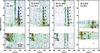 |
Fig. 1 Position-velocity diagram of Hα, [S ii] λ673 nm, and [Fe ii] λ1643 nm in July 2012, and [S ii] λ673 nm in July 2013. The y-axis denotes the position along the slit; y > 0 corresponds to the NE lobe, while y < 0 corresponds to the SW lobe. Due to the brightness of the source, the central region was not observed. Black contours correspond to log Fλ/ [erg s-1 cm-2Å-1] = (−17.5, −17, −16.5, −16, −15.5). The blue contours indicate the 3σ detection level of the knots. The black crosses denote the derived positions and velocities of the knots, and their 1σ uncertainties. Note the bow shock features in knot A and C in Hα. |
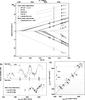 |
Fig. 2 a) Positions of the knots of HH 409 over time; vertical bars correspond to the FWHM of the spatial profile. The shaded bands and dashed lines are linear fits to their trajectories. The arrows represent the velocities on the sky calculated from the radial velocities and disk inclination. References: (1) Devine et al. (2000); (2) Grady et al. (2000); (3) Wassell et al. (2006); (4) Günther et al. (2013); (5) Klaassen et al. (2013). b) Launch epochs from radial velocities in the X-shooter spectra. Every symbol represents the flux (on a logarithmic scale) and tlaunch of one row of the two-dimensional spectrum, obtained through the procedure described in the text. Only peaks above the 3σ background level are displayed. The data show a periodicity of 16 yr, which was also obtained from the global fit to the jet proper motions (dotted lines). The launch epochs also agree well between the blue and red lobes. c) Launch epochs of knots in the blue (open squares) and red (closed squares) lobes, derived from proper motions and from radial velocities. The dotted horizontal lines are plotted on a 16-year interval; note the logarithmic scale. |
3. Results: the jet
W06 present an overview of HST data of the jet. It has a position angle of 42.5 ± 3.5° (north through east) and extends up to 30′′ in both the southwest (blue-shifted, or “blue lobe”) and northeast (“red lobe”) direction. This section contains an analysis of the X-shooter spectra of the jet. It is divided into two parts: the kinematics and the physical conditions.
3.1. Kinematics: proper motions vs. radial velocities
The bipolar HH 409 jet consists of a sequence of local emission line maxima, or “knots” (Fig. 1). These knots are detected in 40 emission lines of various allowed and forbidden transitions: H i, [C i], [N ii], [O i], [O ii], [S ii], Ca ii, [Ca ii], [Fe ii], and [Ni ii]. No H2 emission is observed along the jet. Fig. 1 displays the X-shooter spectrum of the Hα, [S ii] λ673 nm, and [Fe ii] λ1643 nm emission lines. Knots A, A2, B, C, D, E, F, G, and the onset of H, defined by W06, are indicated in this 2D spectrum. The knot positions are identified by co-adding the position-velocity diagrams of a selection of the strongest emission lines. Two more recently ejected knots: A3 (identified in this work) and B2 (also reported by G13) are only partly covered by the X-shooter slit in July 2012. The movements of these knots are determined from the July 2013 observations and the observations of the Lyα counterpart of knot B2 (G13) and the molecular counterpart of A3 (Klaassen et al. 2013). The jet lobes are asymmetric, the blue lobe being faster (220 − 300 km s-1) than the red lobe (130−200 km s-1). Bow-shock features in knot A and C, which are spatially resolved in the HST images (W06), show up as sharp velocity drops in the X-shooter Hα position-velocity diagram.
Figure 2a shows the measured positions (xt) and lengths (estimated as the FWHM of the spatial profiles along the jet axis) of the knots observed over the 1998−2013 epoch. The trajectories of knots A, A2, B, and C are well fitted by uniform motion. The trajectories of knots A3, B2, and D−G, though poorly constrained, are similar to the other knots. Assuming constant motion for all knots allows us to make an estimate of their launch epochs (tlaunch). These epochs should then be viewed as the intervals during which the bright knots have formed in the jet, close to the driving source.
Since the knots are regularly spaced, a better constraint on their trajectories is obtained by making a global fit to the data presented in Fig. 2a. We assumed that each knot was created simultaneously with its counterpart, that knot creation is periodic, and that knots propagate uniformly on either side of the system. We omitted knot A2 from the fitting procedure, as it has no counterpart. The best-fit model ( ) has a period 16.0 ± 0.7 yr and proper motions vt,red = 0.28 ± 0.01′′ yr-1 and vt,blue = 0.49 ± 0.01′′ yr-1. The global fit is displayed in Fig. A.1.
An independent estimate of the launch epoch estimates is achieved by using X-shooter radial velocities (νr) and assuming that the jet is perpendicular to the disk equatorial plane. Existing estimates of the disk inclination are based on interferometry of the outer disk (idisk = 46 ± 4°, Isella et al. 2007; idisk = 44°, Rosenfeld et al. 2013) and the inner disk (idisk = 48 ± 2°, Tannirkulam et al. 2008a). In this paper we adopt the latter value. From the co-added position-velocity diagrams (Fig. 1) of the brightest lines, a spectral profile is extracted at every pixel of width  along the slit. A Gaussian function is fitted to this profile; its centroid velocity is converted to a launch epochs as tlaunch = xt/(νrtanidisk). The fluxes and launch epochs of these individual components are displayed in Fig. 2b. The 16-year periodicity in the jet structure, as well as the concurrence of knots in both lobes are evident from this figure.
Figure 2a (arrows) and 2c illustrate the agreement in the launch epoch estimates between the proper motion and radial velocity methods. The latter figure also demonstrates the periodicity and simultaneity (in both lobes) of the launch events. The jet inclination angle calculated from the average jet velocities is ijet = tan-1 ⟨ vt ⟩ / ⟨ vr ⟩ = 47 ± 2°. The red-shifted knots B2, B, and C are launched simultaneously with the blue-shifted knots A3, A, and H, respectively. For knot H, tlaunch is estimated from its position in 2004 and the average νr in the blue lobe. Due to their high velocities, the counterparts of the red-shifted knots D, E, F, and G are probably located tens of arcseconds beyond knot H in the blue lobe and are not covered by our observations. The most recent launch epoch traced by our observations peaked in 2001−2004, marking the formation of knots A3 and B2. In the remainder of this paper, we adopt the tlaunch estimates from radial velocities, as these have the smallest measurement error.
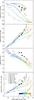 |
Fig. 3 Emission line ratios for six knots in the blue (open symbols) and red (filled symbols) lobes. Contours indicate the predicted ratios by the models of Hartigan et al. (1994) for a grid of pre-shock densities, magnetic field strengths, and shock velocities. The colored symbols correspond to models with νshock = (15,20,25,30,35,40,50,60,70,80,90,100) km s-1. |
3.2. Physical conditions
The line emission along the jet is a result of collisional excitation in shock fronts. Conditions may vary significantly between the regions up- and downstream of the shock front (“pre”- and “post”-shock, respectively; Hartigan et al. 1994). The physical conditions of the shocked gas in the knots (post-shock electron density and total density, ne,post, nH,post; temperature, Te; and ionization, Xe) can be estimated by comparing observed line ratios with those predicted by collisional excitation models (Bacciotti & Eislöffel 1999; for an application to X-shooter spectra see e.g., Ellerbroek et al. 2013). Similarly, the pre-shock parameters (shock velocity, νshock; pre-shock density nH,pre; and magnetic field, B) can be obtained by comparing line ratios to shock models (e.g., Hartigan et al. 1994).
The results presented in this section are summarized in Table 2. We consider the emission >3σ above the background noise. This is the case for knots A, A2, and A3 in the blue lobe and B, C, and D in the red lobe. The line flux per knot is obtained by integrating over the blue contours seen in Fig. 1. We consider only the high-velocity emission. We did not correct for the spatial extent of the knots beyond the slit aperture, which we assume to be low-velocity emission. The line fluxes predicted by models and used in diagnostics in this section are corrected to match the solar abundances of Asplund et al. (2005), which results in a scaling of typically 0.1 dex.
3.2.1. Extinction
Extinction by dust affects the observed line ratios and hence the estimated physical and shock parameters. The value of AV can be estimated by considering forbidden lines from the same upper level which are far apart in the spectrum. [Fe ii] infrared lines are well suited for this purpose, although large uncertainties in the Einstein coefficients affect the outcome (see Nisini et al. 2005, for a discussion). Alternatively H i lines can be used, but their ratios also depend on other model parameters, like the shock velocity (Hartigan et al. 1994).
We find that within the errors the [Fe ii] 1643/1321 nm and 1643/1256 nm line ratios are consistent with theoretical ones computed for AV = 0. Similarly, the Hα/Hβ line ratios follow the predictions from the Hartigan et al. (1994) shock models for the observed range in νshock (see Sect. 3.2.3). Thus, we adopt AV = 0 in the knots along the jet. This is consistent (assuming a normal dust-to-gas ratio in the ISM) with the absence of interstellar (gas) features in the spectrum of the central source and the jet (Finkenzeller & Mundt 1984; Devine et al. 2000), as well as the low on-source extinction measured from photometry (see Sect. 4.1).
3.2.2. Electron density, ionization fraction, electron temperature
The electron density, hydrogen ionization fraction, and electron temperature of the shocked gas in the knots are calculated with the BE method (Bacciotti & Eislöffel 1999). We find an electron density of ~500 cm-3 that decreases along the jet. The ionization fraction is higher in the blue lobe (0.7−0.8) than in the red lobe (0.2−0.4). The electron temperature decreases away from the source and is higher in the blue lobe (Te ~ 1−1.5 × 10⁴ K) than in the red lobe (Te ~ 104 K). Excitation conditions are thus higher in the blue lobe than in the red lobe.
These trends are similar to those found by W06 and G13, although the values for ne,post found by these authors are an order of magnitude higher than our calculations. This can be due to the fact that the slit used in these studies (with a width of  ) only samples the central region of the jet, which probably has a higher density (see, e.g., Bacciotti et al. 2000; Hartigan & Morse 2007). The differences in these and other parameters are consistent within the large uncertainties in the line fluxes measured by these authors. The total density in the post-shock region is estimated as nH,post = ne,post/Xe, under the assumption that hydrogen atoms are the main donor of free electrons.
3.2.3. Shock velocity, magnetic field strength, compression
Figure 3 displays the values of a selection of line ratios against those predicted by Hartigan et al. (1994) for a grid of shock models with nH,pre = (102,103,104) cm-3, B = (10,102,103) μG, and νshock = 10−100 km s-1. The observed ratios are best represented by the models with pre-shock electron densities nH,pre = 100 cm-3, while the magnetic field strength B can adopt values of 10 − 100 μG. Finally, the observed line ratios indicate that in the blue lobe the shock velocity is higher (νshock ~ 80−100 km s-1) than in the red lobe (νshock ~ 35−60 km s-1). This is consistent with the higher excitation conditions in the blue lobe (see also W06 and G13).
The pre-shock density is of order 100 cm-3, as indicated by the comparison with shock models. For the estimated shock velocities and a typical magnetic field strength of 30μG, the compression factor, C = nH,post/nH,pre varies between 6 and 20 (Fig. 17 of Hartigan et al. 1994). We adopt C = 13 ± 7 in all the knots. The average density is estimated as the geometric mean of pre- and post-shock densities. This can be expressed in terms of the post-shock conditions and the compression factor as 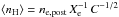 (Hartigan et al. 1994). The resulting total number density in the jet is of order 100 cm-3. The [S ii]/Hα ratio in the red lobe is underpredicted by all models except those with n = 1000 cm-3 and B = 1000μG. This may indicate that a strong magnetic field inhibits compression and enhances the emission from lower ionization species.
3.2.4. Mass loss rate
The mass-loss rate Ṁjet is an important parameter in jet physics. It determines the amount of energy and momentum injected in the ISM, and its ratio with the accretion rate reflects the (in-) efficiency of the accretion process. Various methods have been developed to calculate Ṁjet from the physical parameters (for a review, see Dougados et al. 2010). We apply two of these to our dataset: (1) we calculate the mass-loss rate from the jet cross section ( ), total density ⟨ nH ⟩, and velocity (νJ = | νr | /cosi); and (2) from the [S ii] and [O i] line luminosities.
Cross section:
with this method (“BE” method, Bacciotti & Eislöffel 1999), the mass-loss rate is calculated from the average density, velocity, and cross section of the jet:  (1)where we adopt μ = 1.24 for the mean molecular weight. We take the jet radius RJ to be equal to half of the jet FWHM at the selected knot position as measured from resolved HST observations in the [S ii] lines (W06). For the knots considered, RJ increases from 40 au up to 100 au away from the source.
Line luminosities:
if the physical conditions are uniform within each knot, the mass-loss rate is proportional to the number of emitting atoms in the observed volume (Podio et al. 2006, 2009): (2)where Lline is the line luminosity; ν, Ai, and fi are the frequency, radiative rate, and upper level population fraction for the considered transition, respectively. Xi/X is the fraction of atoms of the considered species in the Xi ionization state and X/H the species’ relative abundance with respect to hydrogen. The upper level population, fi, is calculated from the statistical equilibrium equations using the values of ne,post and Te calculated from the line diagnostics. The knot length lt is measured along the slit. This method is applied to two lines: [S ii] λ673 nm and [O i] λ630 nm. We assume that all sulphur is singly ionized. To compute the ionization fraction of oxygen, we consider collisional ionization, simple and dielectronic recombination, and charge exchange with H.
The mass-loss rates calculated from the line luminosities (Table 2) agree with each other within the uncertainties. The values from the cross section method are significantly and systematically lower than these. This discrepancy may be caused by an underestimated magnetic field strength and hence, an overestimated compression factor. Additionally, upon comparison with the Hartigan et al. (1994) models (Fig. 3), the observed [N ii] λ683 nm/[O i] λ630 nm ratios suggest a lower Xe than derived from the BE method, resulting in a higher Ṁjet. The mass-loss rate is constant across each lobe; those found for the red lobe are a factor 2 higher than in the blue lobe. The average mass-loss rate is ⟨ Ṁjet ⟩ = 5 ± 2 × 10⁻¹⁰ M⊙ yr-1.
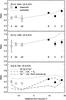 |
Fig. 4 Top two panels: predicted versus observed [Fe ii]/[S ii] ratios, based on the physical conditions derived in Sect. 3.2. Bottom panel: same as above, for [Ca ii]/[S ii]. Predictions are made for the three limiting cases discussed in the text. No evidence is found for depletion of refractory elements in the jet. |
3.2.5. Dust content
The line ratios observed in the jet may also be used to test for depletion of refractory species, such as Ca and Fe. This indicates the presence of dust in the jet launch region. The gas-phase abundance of these species is strongly depleted in the ISM with respect to solar abundances because their atoms are locked onto dust grains (Savage & Sembach 1996). When dust grains evaporate in the launching region or are sputtered in shocks along the jet, these species are released into the gas-phase (Jones et al. 1994; Jones 2000; May et al. 2000; Draine 2004; Guillet et al. 2009, 2011). Gas phase depletion of refractory elements has been observed by Nisini et al. (2005) and Podio et al. (2006, 2009, 2011) in HH jets from Class I sources at large distances from their driving source. It has also been observed in the inner 100 au of a CTTS jet (Agra-Amboage et al. 2011).
In order to check for the presence of dust grains in the jet launch zone, we estimate the Ca and Fe gas-phase abundance following the procedure illustrated in e.g., Nisini et al. (2005) and Podio et al. (2006). We compare observed line ratios of refractory (Ca, Fe) and non-refractory (S) species with ratios computed through the estimated parameters (ne,post, Xe, and Te). We use the flux ratios of [Ca ii] λ729 nm, [Fe ii] λ1256 nm, and [Fe ii] λ1643 nm to [S ii] λ 673 nm (Fig. 4).
We assume that Fe and S are singly ionized and use the 16-levels model presented in Nisini et al. (2002, 2005) with collisional coefficients by Nussbaumer & Storey (1988) for Fe and by Keenan et al. (1996) for S. For the [Ca ii]/[S ii] ratio, it is assumed that no neutral calcium is present, since its ionization potential is very low, 6.1 eV. For the ionization balance we consider three limiting cases:
-
(1)
All calcium is in Ca+. This is most likely an overestimate, as some Ca may be doubly ionized.
-
(2)
The Ca++/Ca+ fraction is equal to the hydrogen ionization fraction, Xe. As explained in Podio et al. (2009), this is justified because the ionization potential of Ca+ is similar to that of hydrogen (11.9 eV and 13.6 eV, respectively). This also goes for the recombination and collisional ionization coefficients for temperatures lower than 3 × 10⁴ K.
-
(3)
The Ca++/Ca+ fraction is calculated by assuming coronal equilibrium at the estimated knot temperature T. Upward transitions are assumed to be due to electron collisions and downward transitions occur by spontaneous emission. This underestimates the Ca+ fraction, as there can be no equilibrium in the jet while the gas is moving.
Figure 4 shows the observed and predicted line ratios. No significant depletion of refractory species is found in the jet knots. Some care should be taken when interpreting this result. The collisional coefficients and atomic parameters for [Fe ii] transitions are affected by large uncertainties (Giannini et al. 2008). The [Fe ii]/[S ii] ratio may be overpredicted if foreground dust is present, which we do not consider likely. The [Fe ii] and [S ii] lines may have different filling factors; the Fe lines could originate in a denser or larger region (see Nisini et al. 2005; Podio et al. 2006). When this is taken into account, one should take the estimated Fe gas abundance as an upper limit. Despite these uncertainties, our analysis gives no indication of dust grains in the launch region of the high-velocity jet.
 |
Fig. 5 Top: lightcurve of HD 163296 in V (0.55 μm) and L (3.76 μm). The dotted line and the gray shaded areas correspond to the mean value and 1σ spread. The time intervals denoted above the V-band lightcurve are expanded in the bottom panel. Horizontal bars indicate the jet launch epochs estimated from radial velocities (Sect. 3.1). Bottom: V-band lightcurve for selected intervals, exhibiting the shape, duration, and frequency of the fading events. The calendar date corresponding to the minimum value on the x-axis is displayed in the bottom left corner of each graph. References for plot symbols: (1) de Winter et al. (2001); (2) Manfroid et al. (1991); (3) Maidanak Observatory (Grankin et al., in prep.); (4) Swiss (this work); (5) Perryman et al. (1997); (6) Hillenbrand et al. (1992); (7) Eiroa et al. (2001); (8) Pojmanski & Maciejewski (2004); (9) AAVSO (this work); (10) Tannirkulam et al. (2008b); (11) Mendigutía et al. (2013); (12) Sitko et al. (2008); (13) de Winter et al. (2001); (14) Berrilli et al. (1992); (15) BASS; (16) SpeX (Sitko et al. 2008, this work). See Table A.1 for more details. |
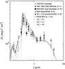 |
Fig. 6 Average SED of HD 163296 (open symbols), fitted with a 9250 K Kurucz model reddened with AV = 0.5; the NIR excess is fitted with a blackbody at 1500 K (the combined model spectrum is shown as a solid gray line). Filled symbols indicate measurements during NIR brightening and optical fading epochs; the number of observations is displayed in brackets. Dash-dotted, dashed, and dotted gray lines represent models reddened with AV = 0.7,0.9, and 1.3, respectively. |
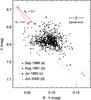 |
Fig. 7 (B − V, V) color−magnitude diagram for HD 163296. Datapoints span the period 1983−2012; see Fig. 5 for the coverage of this epoch. Only points with errors <0.1 mag are plotted. Fading events in 1988, 1991, 1993, and 2000 (letters correspond to Fig. 5) are highlighted with colored symbols. During these events, the colors change along the extinction vector (Cardelli et al. 1989), which is plotted for RV = 3.1 and RV = 5.0. The origin of this vector, indicated with a red cross, represents the intrinsic colors and magnitude of an A1V star at 119 pc (Kenyon & Hartmann 1995). |
4. Results: variability of the central source
In this section we describe the historic lightcurve of the source, as well as the photometric and spectroscopic accretion diagnostics. We adopt the stellar parameters determined by Montesinos et al. (2009), which we find to be consistent with the 2012 X-shooter spectrum. These parameters are the effective temperature Teff = 9250 ± 200 K, stellar radius R∗ = 2.3 ± 0.2R⊙, and mass M∗ = 2.2 ± 0.1 M⊙.
4.1. Photometric variability
A lightcurve of HD 163296 is constructed from the collected data described in Sect. 2.2 and summarized in Table A.1. The top panel of Fig. 5 displays the V- and L-band data for the 1978−2013 epoch. Fig. A.2 displays all the photometric data.
The optical brightness of the source over the period 1980−2012 fluctuates around a steady level (⟨ V ⟩ = 6.93 ± 0.14 mag). Over this period, several fading events are seen, during which the optical brightness decreases significantly. The most prominent of these started in March 2001 and lasted for at least 6 months (up to at most 1.1 yr). Within one month, V increased up to 0.71 ± 0.15 mag above its average value. The bottom panel of Fig. 5 displays a “zoom in” on the lightcurve over this and several other fading events. Fadings of order 0.1 mag occur predominantly in the 2001−2006 epoch with durations from hours to several weeks.
Optical photometric observations dating back as far as the 1890s were obtained from the DASCH catalog (see Grindlay et al. 2012). Since the target was either saturated or in the non-linear domain on most of the photographic plates, we were only able to retrieve lower limits on the photometric measurements. However, prolonged fadings of more than 3σ are observed throughout the lightcurve, indicating that these are recurring events.
In the NIR, the time coverage is much sparser. The mean brightness in the L-band over the 1978–2012 period is ⟨ L ⟩ = 3.36 ± 0.10 mag. The mean brightness level in the H, K, L, and M bands is exceeded by 10% in three epochs: in 1986 (Nobs = 2, see Fig. A.2), 2001–2 (Nobs = 3), and 2011–12 (Nobs = 4). The first two epochs were also reported by Sitko et al. (2008). The 2002 event marked a 30% increase in flux in the L-band. Note, however, that both the measurement error and the intrinsic scatter of the NIR brightness are large. A denser coverage of the lightcurve would be needed to evaluate the significance and uniqueness of such events.
The photometry during fading events is further illustrated in Fig. 6. The average SED was computed by taking the mean of the photometry, omitting measurements that deviate more than 2σ from the mean value. It is fitted with a 9250 K Kurucz model and a blackbody at 1500 K. In the literature, estimates for the extinction deviate from E(B − V) = 0.015 (from the absence of interstellar gas absorption; Devine et al. 2000) up to E(B − V) = 0.15 (from SED fitting; Tilling et al. 2012). The average reddening in our photometric data is E(B − V) = 0.065 ± 0.016 (Fig. 7). For the plot in Fig. 6 we adopt E(B − V) = 0.15 and RV = 3.1, hence AV = 0.5 (Cardelli et al. 1989), which best fits the SED in the UBVRI-bands. The disagreement between the extinction estimates may be explained by a circumstellar extinction carrier with a lower gas-to-dust ratio than in the ISM, variability of its column density, or both. The optical colors during the fading events in 1988, 1991, 1993, and 2000 are well fitted by an enhanced dust extinction of ΔAV ~ 0.2 − 0.4 mag and RV = 3.1 − 5.0 (Fig. 7). The major fading event in 2001, for which colors are not available, implies an enhancement of AV by 0.7−0.8 mag.
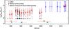 |
Fig. 8 Accretion rate estimates from the Balmer jump (squares: mean; circles: individual measurements) and Brγ luminosity (crosses). Individual measurements through the Balmer jump method have typical errors of 0.5 dex. Jet launch epochs estimated from radial velocities are indicated with horizontal bars (Sect. 3.1). |
The 2002 NIR brightening may have a common origin with the optical fading in 2001. This is further reinforced by the simultaneous measurement of optical fading and NIR brightening in the 2011–2012 X-shooter observations (although large errors affect X-shooter spectro-photometry). We discuss possible explanations for this phenomenon in Sect. 4.2.
4.2. Mass accretion rate
The mass accretion rate, Ṁacc, is an important parameter in characterizing disk evolution and the accretion-ejection process. Despite their generally weak stellar magnetic fields, HAeBe stars show signatures indicative of magnetospheric accretion as also observed in CTTS stars. These include UV excess emission from the accretion shock (Mendigutía et al. 2011; Donehew & Brittain 2011) and emission line profiles showing infall and outflow signatures (Muzerolle et al. 2004).
Estimates of Ṁacc in HD 163296 using these diagnostics are of order 10-8 − 10-7 M⊙ yr-1 and vary over more than an order of magnitude (Garcia Lopez et al. 2006; Eisner et al. 2010; Donehew & Brittain 2011; Mendigutía et al. 2011, 2013). This wide spread is probably in large part due to the use of different interpretative models in these studies. In this section, we synthesize these different measurements by interpreting them within a uniform method. In this way, any detected variability can more reliably be interpreted as being intrinsic. We review time-resolved measurements of two tracers for Ṁacc: Balmer excess and Brγ emission.
The most direct diagnostic for the accretion rate is the UV excess emission measured around the Balmer jump. This emission originates in the accretion shock as a release of gravitational energy of the infalling material. The excess emission can be measured by comparing the observed flux to a photospheric model that corresponds to the stellar spectral type and luminosity. This gives an estimate of the accretion luminosity.
Herbig stars are bright, so any UV excess will have a limited contrast with the photospheric emission. Since the photospheric emission is relatively weak blue-ward of the Balmer jump, the U − B color serves as the best diagnostic for the UV excess. The observed U − B color is corrected for extinction by comparing the observed B − V color with the intrinsic color of an A1V star (Kenyon & Hartmann 1995). The Balmer excess is subsequently obtained by comparing the dereddened value of U − B with the intrinsic color. This value is then converted into Ṁacc using the accretion shock model described in Mendigutía et al. (2011). This was done for the datasets of Maidanak Observatory, ESO Swiss, and Mendigutía et al. (2013); see Table A.1.
The second method to estimate Ṁacc is based on the Brγ line luminosity, L(Brγ). Models predict that the emission lines are formed in the accretion flow (Hartmann et al. 1994). Indeed, a strong correlation is observed between L(Brγ) and accretion luminosity (Muzerolle et al. 1998). This correlation scales up to the intermediate stellar mass regime (Calvet et al. 2004; Mendigutía et al. 2011). We use the correlation coefficients from the latter work (their Eq. (8)) to obtain a rough estimate of Ṁacc.
We derive the Brγ line luminosities from the equivalent width (EWobs) and K measurements available in the literature. The line luminosity is defined as  (3)where
 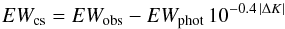 (4)is the line equivalent width with respect to the circumstellar continuum. The last term includes a correction factor for the veiling of photospheric lines by the NIR continuum emission. This factor depends on ΔK, defined as the difference between the observed and the photospheric K-band magnitude (see also Rodgers 2001); for the latter we adopted Kphot = 6.3 mag. Since in most cases no simultaneous extinction measurement was available, we adopted AV = 0.5 ± 0.5 for all observations. A photospheric equivalent width EWphot = −22 Å was assumed (Mendigutía et al. 2013). Table A.2 lists the line luminosities obtained in this way. The corresponding Ṁacc-values are displayed in Fig. 8.
As fortune would have it, before 2001, just Balmer excess measurements are available, and after 2001 just L(Brγ) measurements, with the exception of the five photometric observations in 2011–12. These were made with X-shooter, thus the two described methods to estimate Ṁacc could be simultaneously applied. For a more thorough treatment of the accretion diagnostics of these spectra, we refer to Mendigutía et al. (2013).
In Fig. 8 the measurements from both methods are displayed. The values of Ṁacc from the Balmer excess method show no significant peaks, and level around log Ṁacc = −7.1 ± 0.7 M⊙ yr-1. Much of the large scatter can be accounted for by the statistical error of ~0.6 dex on the individual measurements. Far-UV spectra were taken in 1986–1987 (with IUE) and 1998−2004 (with HST/FUSE and STIS, see also Tilling et al. 2012). The continuum level varies considerably between these measurements. However, the sampling is too sparse to put firm constraints on the accretion rate variability. Within the uncertainties, no significant variation of the accretion rate before 2001 is detected.
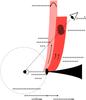 |
Fig. 9 Cartoon drawing of the geometry of the HD 163296 disk-jet system and a scenario that may explain the optical fading and NIR brightening, as discussed in Sect. 5.5. |
The measurements of L(Brγ) in the period 2001−2012 agree well within 2.3 ± 0.3 × 10⁻³L⊙. The subsequently derived estimates of Ṁacc are log Ṁacc = −6.2 ± 0.8 M⊙ yr-1. It appears that Ṁacc has substantially increased after 2001. The high values measured in 2011−12 agree between the two methods. However, the line luminosity tracer probably suffers from large systematical uncertainties, see Sect. 5.3.
5. Discussion
In this section, we summarize the constraints that our observations of HH 409 put on the jet launching mechanism. We discuss the periodicity and asymmetry of the jet, and the mass loss and accretion rates. Also, we consider the origin of the optical fading events and their possible connection with the accretion and jet launching process. A sketch of the system’s proposed geometry is depicted in Fig. 9.
5.1. Periodicity
The excellent agreement between radial velocity and proper motion measurements of the individual knots (Sect. 3.1) confirms that each lobe of the jet is perpendicular to the disk within 4.5°. This is consistent with, but more accurate than previous measurements (Grady et al. 2000, W06).
Over the last decades, bright shock fronts in the high-velocity jet have appeared simultaneously and periodically (period =16.0 ± 0.7 yr) on both sides of the disk. The periodicity of the knot spacings was also noted by W06. The typical error on the launch epochs is a few years; within this uncertainty, they are created simultaneously. Since the sound speed crossing time of the inner disk region (~0.5 au) is also a few years (Raga et al. 2011), the knots are probably causally connected: a single variation in the outflow mechanism in the inner region may have produced a velocity pulse on both sides of the disk. In Sect. 5.5.1 we comment on various explanations for these periodic “launch epochs”.
5.2. Asymmetry
The HH 409 lobes are highly asymmetric in velocity and physical conditions. The average velocity in the blue lobe is a factor 1.5 higher than in the red lobe. This asymmetry is reflected in the physical conditions (Sect. 3.2): in the blue lobe, the material has higher shock velocities and, hence a higher ionization fraction. The mass-loss rate in the blue lobe is a factor 2 lower than in the red lobe. Consequently, the energy input in the jet ( ) is roughly equal in both lobes.
The dispersion in the jet velocity ΔνJ (defined as the deprojected FWHM of the spectral profile across the slit) is higher in the blue lobe, but the relative dispersion ΔνJ/νJ ~ 0.2 is similar in both lobes. Interestingly, the same property is observed in other asymmetric jets (RW Aur, Hartigan & Hillenbrand 2009; DG Tau B, Podio et al. 2011). For all three objects, the relative velocity dispersion is higher than what is expected by projection effects given the jet opening angle (see also Hartigan & Hillenbrand 2009). The latter authors suggest that the dispersion may be caused by magnetic waves. This would imply that despite the asymmetry in velocity, the Alfvénic Mach number MA = νJ/νA is the same in both lobes (and equals ~5 for HD 163296).
Asymmetry in velocity and ionization conditions is a commonly observed (Hirth et al. 1994; Ray et al. 2007) and intriguing property of jets. Various explanations have been proposed, including an asymmetric disk structure or magnetic field configuration, or propagation in an asymmetric environment (Ferreira et al. 2006; Matsakos et al. 2012; Fendt & Sheikhnezami 2013). In some cases, the mass-loss rate is found to be similar in both lobes despite the velocity asymmetry, suggesting external conditions cause their different appearance (Melnikov et al. 2009; Podio et al. 2011). In other systems, like HH 1042 (Ellerbroek et al. 2013), the mean velocity and mass-loss rate are similar on both sides, but velocity modulations are different, indicating a non-synchronized launching mechanism.
In the case of HD 163296 the similar energy input and simultaneous launching epochs suggest that a single driving mechanism controls jet launching on both sides of the disk. The lobes are asymmetric already close to the source (G13), and no strong density gradients are observed in the surrounding medium (Finkenzeller & Mundt 1984). The asymmetry may then be the effect of differing conditions in the launching or acceleration regions of each jet lobe.
5.3. Mass loss and accretion rate
We have measured mass outflow rates of Ṁjet = 0.2 − 1 × 10⁻⁹ M⊙ yr-1 in the different knots. This is one order of magnitude lower than some of the estimates of W06 and G13. However, the uncertainties in these earlier measurements are quite large because of the low S/N of the spectra used. The absolute value of Ṁjet is up to two orders of magnitude lower than sources with similar masses and accretion rates (Melnikov et al. 2008, 2009; Agra-Amboage et al. 2009, 2011). In these studies, the mass flux is obtained within a few arcseconds from the source. We measure fluxes further from the source, where outer streamlines may carry a substantial fraction of the mass. This results in underestimating both the line luminosities and the jet cross section.
The ratio Ṁjet/Ṁacc is an observable which differentiates theoretical models of jet launching. Measuring it, however, is difficult. Apart from the large systematic uncertainties in the measurements of both Ṁjet and Ṁacc, there is a fundamental issue affecting their comparison. While the accretion rate is measured on source, the mass outflow rate is usually measured in a knot at a distance from the source where it is spatially resolved. The material in this knot has been ejected some time in the past. Moreover, the shocked knot is probably the outcome of an episode of increased accretion activity. Hence, comparing these two measurements probably does not reflect their true ratio at the time of ejection. Such a measurement may be achieved if Ṁacc is measured during the creation of a knot. The knot itself should then be observed around one year later, when it can be spatially resolved (but is still reasonably close to the source) to estimate Ṁjet.
Our data allow us to make such an estimate. The combined mass-loss rate in knots A and B is Ṁjet = 1.3 ± 0.6 × 10⁻⁹ M⊙ yr-1. These knots were created in 1983−1988 (Fig. 2). During this period the accretion rate averaged Ṁacc = 7.8 ± 4.2 × 10⁻⁸ M⊙ yr-1 (Fig. 8). This implies Ṁjet/Ṁacc is of order 0.01 − 0.1, within the range predicted by theoretical models (e.g., Konigl & Pudritz 2000). The accuracy on this parameter is insufficient to discriminate between different models of jet launching. Averaged over all knots and epochs, Ṁjet/Ṁacc ≲ 0.01, which may be an effect of underestimating the mass-loss rate, as described above.
5.4. Kinematic structure and size of the launch region
The jet consists of a layered structure, with a narrow high-velocity component or jet (detected in atomic lines) and a wide low-velocity component or disk wind (detected in molecular lines). The disk wind is wider (several hundred au at ~5′′ from the source, Klaassen et al. 2013) than the high-velocity jet (less than 100 au, W06). This “onion-like” kinematic structure is similar to what has been observed in other jets (Bacciotti et al. 2000; Pyo et al. 2009; Whelan et al. 2010).
Its low velocity and large radius indicate that the molecular disk wind is launched at larger radii from the central source than the atomic high-velocity jet. This is consistent with predictions from magneto-centrifugal processes, where the velocity in the jet scales with the Keplerian velocity (νK) at the launch radius as (Blandford & Payne 1982): 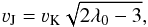 (5)where the magnetic lever arm parameter
  is the squared ratio of the Alfvèn radius and the launch radius. The results of Sect. 3.2.5 suggest that the high-velocity jet is launched within the dust sublimation radius <0.5 au, thus νK ≳ 60 km s-1. Given the observed νJ, a lever arm parameter of λ0 ≲ 14 is expected. This is consistent with the estimated Ṁjet/Ṁacc for a dynamical range in launch radii r0,max/r0,min < 13 (Ferreira et al. 2006, their Eq. (17)).
Observational evidence for a disk wind has been found in this system and in other, similar sources. Many spectral lines in HD 163296 exhibit variability related to outflow on timescales of days (Catala et al. 1989; Tilling et al. 2012). Interferometric observations of the Brγ line show that the emission originates in a region more compact than the continuum, but more extended than the magnetosphere; its most likely origin is a stellar or disk wind (Kraus et al. 2008). Other sources exhibit similar signatures in Brγ, attributed to an equatorial atomic disk wind within a few au of the star (Malbet et al. 2007; Tatulli et al. 2007; Eisner et al. 2010; Benisty et al. 2010b; Weigelt et al. 2011).
The molecular disk wind is probably launched from outside the sublimation radius and may hence transport dust grains off the disk surface. This is a possible explanation for the fading events, see Sect. 5.5.
5.5. Optical fading, NIR brightening: dust in the wind?
We consider dust clouds entrained in a disk wind as the most likely scenario to explain the observed photometric variability episodes. Vinković & Jurkić (2007) propose that this phenomenon may contribute to the infrared variability of young stellar objects. Bans & Königl (2012) adapt it to explain the NIR brightening of HD 163296. Our additional observation of optical fading episodes that are well-fitted by dust extinction strengthens this hypothesis. Given the system’s inclination and the dust-free region inside 0.5 au, an occulting cloud must be lifted to ≳0.5 au above the disk plane in order to cross the observer’s line of sight to the star. The observed diagnostics can be achieved self-consistently with a reasonable set of cloud properties.
The situation is sketched in Fig. 9. A dust cloud is lifted from the disk surface and exposed to direct stellar light. As a result, the dust heats up and emits thermal radiation in the NIR. When the cloud transits the star, the latter will appear fainter to the observer. The launch of the cloud in 2001 coincides with the creation of a shock front (knot A3). This knot propagates through the high-velocity jet and is observed far from the source in 2012.
The amount of thermal radiation received at a distance d from a dust cloud of mass Mc at a wavelength λ in the optically thin limit is: 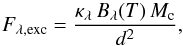 (6)where κλ is the opacity of dust, for which we assume a value of 1.34 × 103 cm2 g-1 in the K-band, given a typical ISM particle size distribution (Mathis et al. 1977). Bλ(T) is the specific intensity of a black-body at the dust temperature, which we assume to be 1500 K. The distance to the observer is d = 120 pc. To match the observed flux increase of 30% in the L-band in 2002, the cloud mass must be Mc ~ 4 × 10-12 M⊙.
Assuming that the cloud is co-moving with the CO disk wind at ~10 km s-1, the observed transit time ttr = 0.6 − 1.1 yr implies a size of 1 − 2 au. For a spherical cloud we obtain a density ρ ~ 10-18 g cm-3. This high value is of the same order as the disk density, suggesting a compact cloud. The optical depth in the V-band over a path length l through a medium with density ρ is  (7)where κV = 1.78 × 103 cm2 g-1 for the assumed particle size distribution. This results in an increase of AV = τ/1.086 with a few tenths of magnitudes during transit. This matches the observed transit depth within an order of magnitude. A more elongated cloud would have to be transported by a wind with higher velocity to match the observed transit time. This would imply a lower density and optical depth than are observed.
An appreciable force is needed to lift the cloud off the disk surface. Based on the estimated Ṁwind and observed vwind (Klaassen et al. 2013), the disk wind is easily capable of dragging the cloud along (Eq. (24) in Kartje et al. 1999, see also Bans & Königl 2012). The weaker fadings highlighted in Fig. 5 may be caused by similar, but smaller clouds lifted off the disk. Alternatively, the dust clouds may be created by condensations in the disk wind (cf. Kenyon et al. 1991; Hartmann et al. 2004).
Additional observations of variability in the 2001−2004 epoch support the dust cloud scenario. Sitko et al. (2008) report an enhancement of the 10 μm silicate feature in the 2002 observations. Wisniewski et al. (2008) find that the disk is significantly brighter in scattered light emission in 2003−2004 as compared to 1998. Tannirkulam et al. (2008b) report that the K-band emitting region in 2003 is larger in size than in 2004−2007. All these signatures are consistent with a variable distribution of dust in the system.
Alternatives to the dust lifting model may be conceived to explain the photometric variability. A non-axisymmetric vertical structure, or warp, in the disk may periodically obscure the central source (cf. Muzerolle et al. 2009; Flaherty et al. 2012; Bouvier et al. 2013). However, given the inclination, the source of the stellar optical fading has to be located at h/r ~ 0.9 (with h the height above the disk surface and r the radial distance from the star). The height of the inner disk of HD 163296 is not expected to exceed h/r = 0.2 (Dominik et al. 2003). The typical scale height of inner disk warps is observed to be h/r ~ 0.3 (Alencar et al. 2010). This disfavors a disk warp as a likely scenario to explain optical fading.
Dust may be lifted higher up through tidal disruption of the disk by a companion on a wide and eccentric orbit (cf. Muzerolle et al. 2013; Rodriguez et al. 2013). During the periastron passage of the companion the accretion and outflow activity in the disk is expected to be enhanced (Artymowicz & Lubow 1996). In the next section we comment on this possibility, which may also underly the periodic structure of the high-velocity jet.
5.5.1. The nature of “launch epochs”
The creation of knots may be achieved by a variable outflow velocity (e.g., Raga et al. 1990; Ellerbroek et al. 2013). We emphasize that the knots should thus not be viewed as “gas bullets”, but rather as shock fronts propagating through a slower medium. Their periodic creation of knots (during the derived “launch epochs”) does not necessarily have to take place in the disk, but it can be the consequence of (quasi-)periodic processes in the star-disk system. These include disk instabilities (e.g., Zhu et al. 2007; D’Angelo & Spruit 2012), the interplay between disk rotation and magnetospheric accretion (Romanova et al. 2012), stellar magnetic cycles (Armitage 1995; Donati et al. 2003) or interaction with a companion (Muzerolle et al. 2013). The periodicity of 16 yr corresponds to a Keplerian orbit at 6 au. A radial-velocity signal of an unseen stellar or planetary companion at this orbit would at most be a few km s-1. This would have gone undetected in current spectroscopic and (NIR and sub-mm) interferometric campaigns.
Comparable (apparent) periodicities in jet structure have been found in the structure of other HH sources in different evolutionary stages on 10−1000 yr timescales (see Ellerbroek et al. 2013, and references therein). This suggests that similar processes that cause jet structure operate in young stellar objects throughout their pre-main sequence evolution. In evolved systems, such as X-ray binaries, long-term variability has been linked with recurring disk instabilities (Dubus et al. 2001; Kaur et al. 2012). Oscillations in the gas disks of Be stars produce variability signals with similar periodicity (Okazaki 1991; Telting & Kaper 1994).
It is a compelling possibility that knot creation in the high-velocity jet and dust launching in the (outer) disk wind are the result of the same process. Some of the optical fading and NIR brightening episodes coincide with knot launch epochs (see Fig. 5): event (a) with the launching of knots A and B; (b) with knot A2; and (e)–(h) with knots B2 and A3. This correlation is not well constrained due to the observed spatial sizes of the knots. In addition, the limited coverage of the photometric observations inhibits us to establish a one-to-one relation between photometric fading/brightening and launch epochs. Also, the “launch period” of 16.0 ± 0.7 yr derived from the spacing and velocities of the knots is not seen in the lightcurve. This prevents us from establishing that one and the same periodic mechanism is responsible for all the jet and photometric variability signatures.
Also, basic jet launching theory predicts a coupling between accretion and ejection activity (Konigl & Pudritz 2000). The kinematic structure of jets may then contain a fossil record of a variable (FU Ori/EX Ori–like) accretion process (Reipurth & Aspin 1997; Caratti o Garatti et al. 2013). In HD 163296, a correlation between accretion variability and the jet launch epochs is not apparent given the poorly constrained estimates of Ṁacc (Fig. 8). As was mentioned above, Kraus et al. (2008) find that a stellar or disk wind very likely contributes significantly to the Brγ profile. This may result in a systematical overestimate of the accretion rate from L(Brγ). The apparent increase of the accretion rate after 2001 (Fig. 8) may be strongly biased by this.
6. Summary and conclusions
In this paper, we have presented a kinematical and physical analysis of the HH 409 jet, and have related this to the historic lightcurve of its driving source HD 163296. The main conclusions of this work are listed below.
-
In the HD 163296 disk-jet system, periods of intensified outflowactivity in the high-velocity jet occur on a regular interval of16.0 ± 0.7 yr.
-
Although physical conditions and mass-loss rates are asymmetric between the two lobes, the energy input is similar and the periodic creation of knots is synchronized. The velocity dispersion scales with the jet velocity in both lobes, regardless of their asymmetry. These observations suggest that the origin of the asymmetry resides close to, but not inside the disk.
-
We observe no evidence for depletion of refractory species with respect to their solar abundances – a proxy for dust formation – in the high-velocity jet. The absence of dust in the high-velocity jet is consistent with a launch region within 0.5 au.
-
Transient optical fading is identified for the first time in this source. This, together with enhanced NIR excess, is consistent with a scenario where dust clouds are launched above the disk plane.
-
Dust ejections coincide with high-velocity atomic jet launch events (although no one-to-one relation can be established). This tentatively suggests a common origin despite their different launch points (e.g., disk instabilities induced by tidal perturbations).
-
A direct correlation between accretion and ejection events could not be established given the large uncertainties in Ṁacc. We do derive Ṁjet/Ṁacc ~ 0.01 − 0.1, which is consistent with magneto-centrifugal models for jet launching.
Jets are rare in the more evolved HAeBe stars; therefore, HD 163296 provides an exceptional opportunity to study the accretion-outflow phenomenon as it scales up to higher masses. The “jet fossil record” allows us to probe outflow variability on unprecedented timescales. Combining this with photometric variability monitoring also facilitates a direct comparison of accretion and outflow properties, leading to a better understanding of the complex jet launching process. This observing strategy is applicable across a very broad range of astrophysical disk-jet systems that show long-term variability, including young stellar objects, X-ray binaries and active galactic nuclei.
Online material
Appendix A: Additional materials
 |
Fig. A.1 Proper motions of the knots in the HH 409 jet. Same as Fig. 2; the dash-dotted lines correspond to the best global fit made to the positions of the knots, with parameters 16.0 ± 0.7 yr and proper motions vt,red = 0.28 ± 0.01′′ yr-1, and vt,blue = 0.49 ± 0.01′′ yr-1. The A2 data are omitted from the fitting procedure. |
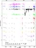 |
Fig. A.2 Lightcurve of HD 163296 compiled from the resources listed in Table A.1. The dotted lines indicate the mean values. References for plot symbols: (1) de Winter et al. (2001); (2) Manfroid et al. (1991); (3) Maidanak Observatory (Grankin et al., in prep.); (4) Swiss (this work); (5) Perryman et al. (1997); (6) Hillenbrand et al. (1992); (7) Eiroa et al. (2001) (8) Pojmanski & Maciejewski (2004); (9) AAVSO (this work); (10) Tannirkulam et al. (2008b); (11) Mendigutía et al. (2013); (12) Sitko et al. (2008); (13) de Winter et al. (2001); (14) Berrilli et al. (1992); (15) BASS; (16) SpeX (Sitko et al. 2008, this work); (17) Kimeswenger et al. (2004); (18) Skrutskie et al. (2006). |
Overview of datasets used in this study.
Mass accretion rate from Brγ luminosity.
Acknowledgments
The referee, Dr. Tom Ray, is acknowledged for useful comments that helped improve the manuscript. The authors thank Myriam Benisty, Jerome Bouvier, Carsten Dominik, Patrick Hartigan, Henny Lamers, Koen Maaskant, Michiel Min, Brunella Nisini, Charlie Qi, Alex Raga, and Rens Waters for discussions about this work. Patrick Hartigan is also acknowledged for kindly providing the shock model results in tabular form. The ESO staff and Christophe Martayan in particular are acknowledged for their careful support of the VLT/X-shooter observations. Daryl Kim is acknowledged for his technical support of the BASS observing runs. The authors thank Bill Vacca, Mike Cushing, and John Rayner for useful discussions on the use of the SpeX instrument and the Spextool processing package. This work was supported by a grant from the Netherlands Research School for Astronomy (NOVA), NASA ADP grants NNH06CC28C and NNX09AC73G, and the IR&D program at The Aerospace Corporation. LP acknowledges the funding from the FP7 Intra-European Marie Curie Fellowship (PIEF-GA-2009-253896).
References
- Agra-Amboage, V., Dougados, C., Cabrit, S., Garcia, P. J. V., & Ferruit, P. 2009, A&A, 493, 1029 [NASA ADS] [CrossRef] [EDP Sciences] [Google Scholar]
- Agra-Amboage, V., Dougados, C., Cabrit, S., & Reunanen, J. 2011, A&A, 532, A59 [NASA ADS] [CrossRef] [EDP Sciences] [Google Scholar]
- Alencar, S. H. P., Teixeira, P. S., Guimarães, M. M., et al. 2010, A&A, 519, A88 [NASA ADS] [CrossRef] [EDP Sciences] [Google Scholar]
- Armitage, P. J. 1995, MNRAS, 274, 1242 [NASA ADS] [Google Scholar]
- Artymowicz, P., & Lubow, S. H. 1996, ApJ, 467, L77 [NASA ADS] [CrossRef] [Google Scholar]
- Asplund, M., Grevesse, N., & Sauval, A. J. 2005, in Cosmic Abundances as Records of Stellar Evolution and Nucleosynthesis, eds. T. G. Barnes, III, & F. N. Bash, ASP Conf. Ser., 336, 25 [Google Scholar]
- Bacciotti, F., & Eislöffel, J. 1999, A&A, 342, 717 [NASA ADS] [Google Scholar]
- Bacciotti, F., Mundt, R., Ray, T. P., et al. 2000, ApJ, 537, L49 [NASA ADS] [CrossRef] [Google Scholar]
- Bai, X.-N., & Stone, J. M. 2013, ApJ, 769, 76 [NASA ADS] [CrossRef] [Google Scholar]
- Bans, A., & Königl, A. 2012, ApJ, 758, 100 [NASA ADS] [CrossRef] [Google Scholar]
- Benisty, M., Natta, A., Isella, A., et al. 2010a, A&A, 511, A74 [NASA ADS] [CrossRef] [EDP Sciences] [Google Scholar]
- Benisty, M., Malbet, F., Dougados, C., et al. 2010b, A&A, 517, L3 [NASA ADS] [CrossRef] [EDP Sciences] [Google Scholar]
- Berrilli, F., Corciulo, G., Ingrosso, G., et al. 1992, ApJ, 398, 254 [NASA ADS] [CrossRef] [Google Scholar]
- Blandford, R. D., & Payne, D. G. 1982, MNRAS, 199, 883 [NASA ADS] [CrossRef] [Google Scholar]
- Bouvier, J., Grankin, K., Ellerbroek, L. E., Bouy, H., & Barrado, D. 2013, A&A, 557, A77 [NASA ADS] [CrossRef] [EDP Sciences] [Google Scholar]
- Brittain, S. D., Simon, T., Najita, J. R., & Rettig, T. W. 2007, ApJ, 659, 685 [NASA ADS] [CrossRef] [Google Scholar]
- Calvet, N., Muzerolle, J., Briceño, C., et al. 2004, AJ, 128, 1294 [NASA ADS] [CrossRef] [Google Scholar]
- Caratti o Garatti, A., Garcia Lopez, R., Weigelt, G., et al. 2013, A&A, 554, A66 [NASA ADS] [CrossRef] [EDP Sciences] [Google Scholar]
- Cardelli, J. A., Clayton, G. C., & Mathis, J. S. 1989, ApJ, 345, 245 [NASA ADS] [CrossRef] [Google Scholar]
- Catala, C., Simon, T., Praderie, F., et al. 1989, A&A, 221, 273 [NASA ADS] [Google Scholar]
- Corcoran, M., & Ray, T. P. 1998, A&A, 336, 535 [NASA ADS] [Google Scholar]
- D’Angelo, C. R., & Spruit, H. C. 2012, MNRAS, 420, 416 [NASA ADS] [CrossRef] [Google Scholar]
- de Gregorio-Monsalvo, I., Ménard, F., Dent, W., et al. 2013, A&A, 557, A133 [NASA ADS] [CrossRef] [EDP Sciences] [Google Scholar]
- Devine, D., Grady, C. A., Kimble, R. A., et al. 2000, ApJ, 542, L115 [NASA ADS] [CrossRef] [Google Scholar]
- de Winter, D., van den Ancker, M. E., Maira, A., et al. 2001, A&A, 380, 609 [NASA ADS] [CrossRef] [EDP Sciences] [Google Scholar]
- Dominik, C., Dullemond, C. P., Waters, L. B. F. M., & Walch, S. 2003, A&A, 398, 607 [NASA ADS] [CrossRef] [EDP Sciences] [Google Scholar]
- Donati, J.-F., Collier Cameron, A., Semel, M., et al. 2003, MNRAS, 345, 1145 [NASA ADS] [CrossRef] [Google Scholar]
- Donehew, B., & Brittain, S. 2011, AJ, 141, 46 [NASA ADS] [CrossRef] [Google Scholar]
- Dougados, C., Bacciotti, F., Cabrit, S., & Nisini, B. 2010, in Lect. Notes Phys. (Berlin: Springer Verlag), eds. P. J. V. Garcia, & J. M. Ferreira, 793, 213 [Google Scholar]
- Draine, B. T. 2004, in The Cold Universe, Saas-Fee Advanced Course 32, eds. A. W. Blain, F. Combes, B. T. Draine, D. Pfenniger, & Y. Revaz, 213 [Google Scholar]
- Dubus, G., Hameury, J.-M., & Lasota, J.-P. 2001, A&A, 373, 251 [NASA ADS] [CrossRef] [EDP Sciences] [Google Scholar]
- Dullemond, C. P., & Monnier, J. D. 2010, ARA&A, 48, 205 [NASA ADS] [CrossRef] [Google Scholar]
- Eiroa, C., Garzón, F., Alberdi, A., et al. 2001, A&A, 365, 110 [NASA ADS] [CrossRef] [EDP Sciences] [Google Scholar]
- Eisner, J. A., Monnier, J. D., Woillez, J., et al. 2010, ApJ, 718, 774 [NASA ADS] [CrossRef] [Google Scholar]
- Ellerbroek, L. E., Podio, L., Kaper, L., et al. 2013, A&A, 551, A5 [NASA ADS] [CrossRef] [EDP Sciences] [Google Scholar]
- Fendt, C., & Sheikhnezami, S. 2013, ApJ, 774, 12 [NASA ADS] [CrossRef] [Google Scholar]
- Ferreira, J., Dougados, C., & Cabrit, S. 2006, A&A, 453, 785 [NASA ADS] [CrossRef] [EDP Sciences] [Google Scholar]
- Finkenzeller, U., & Mundt, R. 1984, A&AS, 55, 109 [NASA ADS] [Google Scholar]
- Flaherty, K. M., Muzerolle, J., Rieke, G., et al. 2012, ApJ, 748, 71 [NASA ADS] [CrossRef] [Google Scholar]
- Garcia Lopez, R., Natta, A., Testi, L., & Habart, E. 2006, A&A, 459, 837 [NASA ADS] [CrossRef] [EDP Sciences] [Google Scholar]
- Giannini, T., Calzoletti, L., Nisini, B., et al. 2008, A&A, 481, 123 [NASA ADS] [CrossRef] [EDP Sciences] [Google Scholar]
- Grady, C. A., Devine, D., Woodgate, B., et al. 2000, ApJ, 544, 895 [Google Scholar]
- Grady, C. A., Woodgate, B., Torres, C. A. O., et al. 2004, ApJ, 608, 809 [NASA ADS] [CrossRef] [Google Scholar]
- Grankin, K. N., Melnikov, S. Y., Bouvier, J., Herbst, W., & Shevchenko, V. S. 2007, A&A, 461, 183 [NASA ADS] [CrossRef] [EDP Sciences] [Google Scholar]
- Grindlay, J., Tang, S., Los, E., & Servillat, M. 2012, in IAU Symp. 285, eds. E. Griffin, R. Hanisch, & R. Seaman, 29 [Google Scholar]
- Guillet, V., Jones, A. P., & Pineau Des Forêts, G. 2009, A&A, 497, 145 [Google Scholar]
- Guillet, V., Pineau Des Forêts, G., & Jones, A. P. 2011, A&A, 527, A123 [NASA ADS] [CrossRef] [EDP Sciences] [Google Scholar]
- Günther, H. M., Schneider, P. C., & Li, Z.-Y. 2013, A&A, 552, A142 (G13) [NASA ADS] [CrossRef] [EDP Sciences] [Google Scholar]
- Hartigan, P., & Hillenbrand, L. 2009, ApJ, 705, 1388 [NASA ADS] [CrossRef] [Google Scholar]
- Hartigan, P., & Morse, J. 2007, ApJ, 660, 426 [NASA ADS] [CrossRef] [Google Scholar]
- Hartigan, P., Morse, J. A., & Raymond, J. 1994, ApJ, 436, 125 [NASA ADS] [CrossRef] [Google Scholar]
- Hartmann, L., Hewett, R., & Calvet, N. 1994, ApJ, 426, 669 [NASA ADS] [CrossRef] [Google Scholar]
- Hartmann, L., Hinkle, K., & Calvet, N. 2004, ApJ, 609, 906 [NASA ADS] [CrossRef] [Google Scholar]
- Hillenbrand, L. A., Strom, S. E., Vrba, F. J., & Keene, J. 1992, ApJ, 397, 613 [NASA ADS] [CrossRef] [Google Scholar]
- Hirth, G. A., Mundt, R., Solf, J., & Ray, T. P. 1994, ApJ, 427, L99 [NASA ADS] [CrossRef] [Google Scholar]
- Isella, A., Testi, L., Natta, A., et al. 2007, A&A, 469, 213 [CrossRef] [EDP Sciences] [Google Scholar]
- Jones, A. P. 2000, J. Geophys. Res., 105, 10257 [NASA ADS] [CrossRef] [Google Scholar]
- Jones, A. P., Tielens, A. G. G. M., Hollenbach, D. J., & McKee, C. F. 1994, ApJ, 433, 797 [NASA ADS] [CrossRef] [Google Scholar]
- Kama, M., Min, M., & Dominik, C. 2009, A&A, 506, 1199 [NASA ADS] [CrossRef] [EDP Sciences] [Google Scholar]
- Kartje, J. F., Königl, A., & Elitzur, M. 1999, ApJ, 513, 180 [NASA ADS] [CrossRef] [Google Scholar]
- Kaur, R., Kaper, L., Ellerbroek, L. E., et al. 2012, ApJ, 746, L23 [NASA ADS] [CrossRef] [Google Scholar]
- Keenan, F. P., Aller, L. H., Bell, K. L., et al. 1996, MNRAS, 281, 1073 [NASA ADS] [Google Scholar]
- Kenyon, S. J., & Hartmann, L. 1995, ApJS, 101, 117 [NASA ADS] [CrossRef] [Google Scholar]
- Kenyon, S. J., Hartmann, L. W., & Kolotilov, E. A. 1991, PASP, 103, 1069 [NASA ADS] [CrossRef] [Google Scholar]
- Kimeswenger, S., Lederle, C., Richichi, A., et al. 2004, A&A, 413, 1037 [NASA ADS] [CrossRef] [EDP Sciences] [Google Scholar]
- Klaassen, P. D., Juhasz, A., Mathews, G. S., et al. 2013, A&A, 555, A73 [NASA ADS] [CrossRef] [EDP Sciences] [Google Scholar]
- Konigl, A., & Pudritz, R. E. 2000, in Protostars and Planets IV (Tucson: University of Arizona press), 759 [Google Scholar]
- Kraus, S., Hofmann, K.-H., Benisty, M., et al. 2008, A&A, 489, 1157 [NASA ADS] [CrossRef] [EDP Sciences] [Google Scholar]
- Malbet, F., Benisty, M., de Wit, W.-J., et al. 2007, A&A, 464, 43 [NASA ADS] [CrossRef] [EDP Sciences] [Google Scholar]
- Manfroid, J., Sterken, C., Bruch, A., et al. 1991, A&AS, 87, 481 [NASA ADS] [Google Scholar]
- Mathis, J. S., Rumpl, W., & Nordsieck, K. H. 1977, ApJ, 217, 425 [NASA ADS] [CrossRef] [Google Scholar]
- Matsakos, T., Vlahakis, N., Tsinganos, K., et al. 2012, A&A, 545, A53 [NASA ADS] [CrossRef] [EDP Sciences] [Google Scholar]
- May, P. W., Pineau des Forêts, G., Flower, D. R., et al. 2000, MNRAS, 318, 809 [NASA ADS] [CrossRef] [Google Scholar]
- Meeus, G., Montesinos, B., Mendigutía, I., et al. 2012, A&A, 544, A78 [NASA ADS] [CrossRef] [EDP Sciences] [Google Scholar]
- Melnikov, S., Woitas, J., Eislöffel, J., et al. 2008, A&A, 483, 199 [NASA ADS] [CrossRef] [EDP Sciences] [Google Scholar]
- Melnikov, S. Y., Eislöffel, J., Bacciotti, F., Woitas, J., & Ray, T. P. 2009, A&A, 506, 763 [NASA ADS] [CrossRef] [EDP Sciences] [Google Scholar]
- Mendigutía, I., Calvet, N., Montesinos, B., et al. 2011, A&A, 535, A99 [NASA ADS] [CrossRef] [EDP Sciences] [Google Scholar]
- Mendigutía, I., Brittain, S., Eiroa, C., et al. 2013, ApJ, 776, 44 [NASA ADS] [CrossRef] [Google Scholar]
- Modigliani, A., Goldoni, P., Royer, F., et al. 2010, Observatory Operations: Strategies, Proc. SPIE 7737, 773728 [Google Scholar]
- Montesinos, B., Eiroa, C., Mora, A., & Merín, B. 2009, A&A, 495, 901 [NASA ADS] [CrossRef] [EDP Sciences] [Google Scholar]
- Muzerolle, J., Hartmann, L., & Calvet, N. 1998, AJ, 116, 2965 [NASA ADS] [CrossRef] [Google Scholar]
- Muzerolle, J., D’Alessio, P., Calvet, N., & Hartmann, L. 2004, ApJ, 617, 406 [NASA ADS] [CrossRef] [Google Scholar]
- Muzerolle, J., Flaherty, K., Balog, Z., et al. 2009, ApJ, 704, L15 [NASA ADS] [CrossRef] [Google Scholar]
- Muzerolle, J., Furlan, E., Flaherty, K., Balog, Z., & Gutermuth, R. 2013, Nature, 493, 378 [NASA ADS] [CrossRef] [Google Scholar]
- Nisini, B., Caratti o Garatti, A., Giannini, T., & Lorenzetti, D. 2002, A&A, 393, 1035 [Google Scholar]
- Nisini, B., Bacciotti, F., Giannini, T., et al. 2005, A&A, 441, 159 [NASA ADS] [CrossRef] [EDP Sciences] [Google Scholar]
- Nussbaumer, H., & Storey, P. J. 1988, A&A, 200, L25 [NASA ADS] [Google Scholar]
- Okazaki, A. T. 1991, PASJ, 43, 75 [NASA ADS] [Google Scholar]
- Oudmaijer, R. D., Palacios, J., Eiroa, C., et al. 2001, A&A, 379, 564 [NASA ADS] [CrossRef] [EDP Sciences] [Google Scholar]
- Perryman, M. A. C., Lindegren, L., Kovalevsky, J., et al. 1997, A&A, 323, L49 [NASA ADS] [Google Scholar]
- Podio, L., Bacciotti, F., Nisini, B., et al. 2006, A&A, 456, 189 [NASA ADS] [CrossRef] [EDP Sciences] [Google Scholar]
- Podio, L., Medves, S., Bacciotti, F., Eislöffel, J., & Ray, T. 2009, A&A, 506, 779 [NASA ADS] [CrossRef] [EDP Sciences] [Google Scholar]
- Podio, L., Eislöffel, J., Melnikov, S., Hodapp, K. W., & Bacciotti, F. 2011, A&A, 527, A13 [NASA ADS] [CrossRef] [EDP Sciences] [Google Scholar]
- Pojmanski, G., & Maciejewski, G. 2004, Acta Astron., 54, 153 [NASA ADS] [CrossRef] [Google Scholar]
- Pyo, T.-S., Hayashi, M., Kobayashi, N., Terada, H., & Tokunaga, A. T. 2009, ApJ, 694, 654 [NASA ADS] [CrossRef] [Google Scholar]
- Qi, C., D’Alessio, P., Öberg, K. I., et al. 2011, ApJ, 740, 84 [NASA ADS] [CrossRef] [Google Scholar]
- Raga, A. C., Binette, L., Canto, J., & Calvet, N. 1990, ApJ, 364, 601 [NASA ADS] [CrossRef] [Google Scholar]
- Raga, A. C., Noriega-Crespo, A., Lora, V., Stapelfeldt, K. R., & Carey, S. J. 2011, ApJ, 730, L17 [NASA ADS] [CrossRef] [Google Scholar]
- Ray, T., Dougados, C., Bacciotti, F., Eislöffel, J., & Chrysostomou, A. 2007, in Protostars and Planets V (Tucson: University of Arizona press), 231 [Google Scholar]
- Rayner, J. T., Toomey, D. W., Onaka, P. M., et al. 2003, PASP, 115, 362 [NASA ADS] [CrossRef] [Google Scholar]
- Rees, M. J. 1978, MNRAS, 184, 61P [NASA ADS] [CrossRef] [Google Scholar]
- Reipurth, B., & Aspin, C. 1997, AJ, 114, 2700 [NASA ADS] [CrossRef] [Google Scholar]
- Rodgers, B. M. 2001, Ph.D. Thesis, University of Washington [Google Scholar]
- Rodriguez, J. E., Pepper, J., Stassun, K. G., et al. 2013, AJ, 146, 112 [NASA ADS] [CrossRef] [Google Scholar]
- Romanova, M. M., Ustyugova, G. V., Koldoba, A. V., & Lovelace, R. V. E. 2012, MNRAS, 421, 63 [NASA ADS] [Google Scholar]
- Rosenfeld, K. A., Andrews, S. M., Hughes, A. M., Wilner, D. J., & Qi, C. 2013, ApJ, 774, 16 [NASA ADS] [CrossRef] [Google Scholar]
- Savage, B. D., & Sembach, K. R. 1996, ARA&A, 34, 279 [NASA ADS] [CrossRef] [Google Scholar]
- Sitko, M. L., Carpenter, W. J., Kimes, R. L., et al. 2008, ApJ, 678, 1070 [NASA ADS] [CrossRef] [Google Scholar]
- Sitko, M. L., Day, A. N., Kimes, R. L., et al. 2012, ApJ, 745, 29 [NASA ADS] [CrossRef] [Google Scholar]
- Skrutskie, M. F., Cutri, R. M., Stiening, R., et al. 2006, AJ, 131, 1163 [NASA ADS] [CrossRef] [Google Scholar]
- Swartz, D. A., Drake, J. J., Elsner, R. F., et al. 2005, ApJ, 628, 811 [NASA ADS] [CrossRef] [Google Scholar]
- Tannirkulam, A., Monnier, J. D., Millan-Gabet, R., et al. 2008a, ApJ, 677, L51 [NASA ADS] [CrossRef] [Google Scholar]
- Tannirkulam, A., Monnier, J. D., Harries, T. J., et al. 2008b, ApJ, 689, 513 [NASA ADS] [CrossRef] [Google Scholar]
- Tatulli, E., Isella, A., Natta, A., et al. 2007, A&A, 464, 55 [NASA ADS] [CrossRef] [EDP Sciences] [Google Scholar]
- Telting, J. H., & Kaper, L. 1994, A&A, 284, 515 [NASA ADS] [Google Scholar]
- Tilling, I., Woitke, P., Meeus, G., et al. 2012, A&A, 538, A20 [NASA ADS] [CrossRef] [EDP Sciences] [Google Scholar]
- van den Ancker, M. E., Bouwman, J., Wesselius, P. R., et al. 2000, A&A, 357, 325 [NASA ADS] [Google Scholar]
- van Leeuwen, F. 2007, A&A, 474, 653 [NASA ADS] [CrossRef] [EDP Sciences] [Google Scholar]
- Vernet, J., Dekker, H., D’Odorico, S., et al. 2011, A&A, 536, A105 [NASA ADS] [CrossRef] [EDP Sciences] [Google Scholar]
- Vinković, D., & Jurkić, T. 2007, ApJ, 658, 462 [NASA ADS] [CrossRef] [Google Scholar]
- Vinković, D., Ivezić, Ž., Jurkić, T., & Elitzur, M. 2006, ApJ, 636, 348 [NASA ADS] [CrossRef] [Google Scholar]
- Wassell, E. J., Grady, C. A., Woodgate, B., Kimble, R. A., & Bruhweiler, F. C. 2006, ApJ, 650, 985 (W06) [NASA ADS] [CrossRef] [Google Scholar]
- Weigelt, G., Grinin, V. P., Groh, J. H., et al. 2011, A&A, 527, A103 [NASA ADS] [CrossRef] [EDP Sciences] [Google Scholar]
- Whelan, E. T., Dougados, C., Perrin, M. D., et al. 2010, ApJ, 720, L119 [NASA ADS] [CrossRef] [Google Scholar]
- Wisniewski, J. P., Clampin, M., Grady, C. A., et al. 2008, ApJ, 682, 548 [NASA ADS] [CrossRef] [Google Scholar]
- Zhu, Z., Hartmann, L., Calvet, N., et al. 2007, ApJ, 669, 483 [NASA ADS] [CrossRef] [Google Scholar]
All Tables
All Figures
|
Fig. 1 Position-velocity diagram of Hα, [S ii] λ673 nm, and [Fe ii] λ1643 nm in July 2012, and [S ii] λ673 nm in July 2013. The y-axis denotes the position along the slit; y > 0 corresponds to the NE lobe, while y < 0 corresponds to the SW lobe. Due to the brightness of the source, the central region was not observed. Black contours correspond to log Fλ/ [erg s-1 cm-2Å-1] = (−17.5, −17, −16.5, −16, −15.5). The blue contours indicate the 3σ detection level of the knots. The black crosses denote the derived positions and velocities of the knots, and their 1σ uncertainties. Note the bow shock features in knot A and C in Hα. |
| In the text | |
|
Fig. 2 a) Positions of the knots of HH 409 over time; vertical bars correspond to the FWHM of the spatial profile. The shaded bands and dashed lines are linear fits to their trajectories. The arrows represent the velocities on the sky calculated from the radial velocities and disk inclination. References: (1) Devine et al. (2000); (2) Grady et al. (2000); (3) Wassell et al. (2006); (4) Günther et al. (2013); (5) Klaassen et al. (2013). b) Launch epochs from radial velocities in the X-shooter spectra. Every symbol represents the flux (on a logarithmic scale) and tlaunch of one row of the two-dimensional spectrum, obtained through the procedure described in the text. Only peaks above the 3σ background level are displayed. The data show a periodicity of 16 yr, which was also obtained from the global fit to the jet proper motions (dotted lines). The launch epochs also agree well between the blue and red lobes. c) Launch epochs of knots in the blue (open squares) and red (closed squares) lobes, derived from proper motions and from radial velocities. The dotted horizontal lines are plotted on a 16-year interval; note the logarithmic scale. |
| In the text | |
|
Fig. 3 Emission line ratios for six knots in the blue (open symbols) and red (filled symbols) lobes. Contours indicate the predicted ratios by the models of Hartigan et al. (1994) for a grid of pre-shock densities, magnetic field strengths, and shock velocities. The colored symbols correspond to models with νshock = (15,20,25,30,35,40,50,60,70,80,90,100) km s-1. |
| In the text | |
|
Fig. 4 Top two panels: predicted versus observed [Fe ii]/[S ii] ratios, based on the physical conditions derived in Sect. 3.2. Bottom panel: same as above, for [Ca ii]/[S ii]. Predictions are made for the three limiting cases discussed in the text. No evidence is found for depletion of refractory elements in the jet. |
| In the text | |
|
Fig. 5 Top: lightcurve of HD 163296 in V (0.55 μm) and L (3.76 μm). The dotted line and the gray shaded areas correspond to the mean value and 1σ spread. The time intervals denoted above the V-band lightcurve are expanded in the bottom panel. Horizontal bars indicate the jet launch epochs estimated from radial velocities (Sect. 3.1). Bottom: V-band lightcurve for selected intervals, exhibiting the shape, duration, and frequency of the fading events. The calendar date corresponding to the minimum value on the x-axis is displayed in the bottom left corner of each graph. References for plot symbols: (1) de Winter et al. (2001); (2) Manfroid et al. (1991); (3) Maidanak Observatory (Grankin et al., in prep.); (4) Swiss (this work); (5) Perryman et al. (1997); (6) Hillenbrand et al. (1992); (7) Eiroa et al. (2001); (8) Pojmanski & Maciejewski (2004); (9) AAVSO (this work); (10) Tannirkulam et al. (2008b); (11) Mendigutía et al. (2013); (12) Sitko et al. (2008); (13) de Winter et al. (2001); (14) Berrilli et al. (1992); (15) BASS; (16) SpeX (Sitko et al. 2008, this work). See Table A.1 for more details. |
| In the text | |
|
Fig. 6 Average SED of HD 163296 (open symbols), fitted with a 9250 K Kurucz model reddened with AV = 0.5; the NIR excess is fitted with a blackbody at 1500 K (the combined model spectrum is shown as a solid gray line). Filled symbols indicate measurements during NIR brightening and optical fading epochs; the number of observations is displayed in brackets. Dash-dotted, dashed, and dotted gray lines represent models reddened with AV = 0.7,0.9, and 1.3, respectively. |
| In the text | |
|
Fig. 7 (B − V, V) color−magnitude diagram for HD 163296. Datapoints span the period 1983−2012; see Fig. 5 for the coverage of this epoch. Only points with errors <0.1 mag are plotted. Fading events in 1988, 1991, 1993, and 2000 (letters correspond to Fig. 5) are highlighted with colored symbols. During these events, the colors change along the extinction vector (Cardelli et al. 1989), which is plotted for RV = 3.1 and RV = 5.0. The origin of this vector, indicated with a red cross, represents the intrinsic colors and magnitude of an A1V star at 119 pc (Kenyon & Hartmann 1995). |
| In the text | |
|
Fig. 8 Accretion rate estimates from the Balmer jump (squares: mean; circles: individual measurements) and Brγ luminosity (crosses). Individual measurements through the Balmer jump method have typical errors of 0.5 dex. Jet launch epochs estimated from radial velocities are indicated with horizontal bars (Sect. 3.1). |
| In the text | |
|
Fig. 9 Cartoon drawing of the geometry of the HD 163296 disk-jet system and a scenario that may explain the optical fading and NIR brightening, as discussed in Sect. 5.5. |
| In the text | |
|
Fig. A.1 Proper motions of the knots in the HH 409 jet. Same as Fig. 2; the dash-dotted lines correspond to the best global fit made to the positions of the knots, with parameters 16.0 ± 0.7 yr and proper motions vt,red = 0.28 ± 0.01′′ yr-1, and vt,blue = 0.49 ± 0.01′′ yr-1. The A2 data are omitted from the fitting procedure. |
| In the text | |
|
Fig. A.2 Lightcurve of HD 163296 compiled from the resources listed in Table A.1. The dotted lines indicate the mean values. References for plot symbols: (1) de Winter et al. (2001); (2) Manfroid et al. (1991); (3) Maidanak Observatory (Grankin et al., in prep.); (4) Swiss (this work); (5) Perryman et al. (1997); (6) Hillenbrand et al. (1992); (7) Eiroa et al. (2001) (8) Pojmanski & Maciejewski (2004); (9) AAVSO (this work); (10) Tannirkulam et al. (2008b); (11) Mendigutía et al. (2013); (12) Sitko et al. (2008); (13) de Winter et al. (2001); (14) Berrilli et al. (1992); (15) BASS; (16) SpeX (Sitko et al. 2008, this work); (17) Kimeswenger et al. (2004); (18) Skrutskie et al. (2006). |
| In the text | |
Current usage metrics show cumulative count of Article Views (full-text article views including HTML views, PDF and ePub downloads, according to the available data) and Abstracts Views on Vision4Press platform.
Data correspond to usage on the plateform after 2015. The current usage metrics is available 48-96 hours after online publication and is updated daily on week days.
Initial download of the metrics may take a while.