| Issue |
A&A
Volume 562, February 2014
|
|
|---|---|---|
| Article Number | A88 | |
| Number of page(s) | 21 | |
| Section | Extragalactic astronomy | |
| DOI | https://doi.org/10.1051/0004-6361/201322544 | |
| Published online | 11 February 2014 | |
Molecular hydrogen in the zabs = 2.66 damped Lyman-α absorber towards Q J 0643−5041⋆,⋆⋆,⋆⋆⋆
Physical conditions and limits on the cosmological variation of the proton-to-electron mass ratio
1 Institut d’Astrophysique de Paris, UMR 7095 CNRS, Université Pierre et Marie Curie, 98bis boulevard Arago, 75014 Paris, France
e-mail: This email address is being protected from spambots. You need JavaScript enabled to view it.
2 Inter-University Centre for Astronomy and Astrophysics, Post Bag 4, Ganeshkhind, 411 007 Pune, India
3 School of Astronomy, Institute for Research in Fundamental Sciences (IPM), PO Box 19395-5531 Tehran, Iran
4 European Southern Observatory, Alonso de Córdova 3107, Casilla 19001, Vitacura, Santiago, Chile
Received: 26 August 2013
Accepted: 31 October 2013
Abstract
Context. Molecular hydrogen in the interstellar medium (ISM) of high-redshift galaxies can be detected directly from its UV absorption imprinted in the spectrum of background quasars. Associated absorption from H i and metals allow for the study of the chemical enrichment of the gas, while the analysis of excited species and molecules make it possible to infer the physical state of the ISM gas. In addition, given the numerous H2 lines usually detected, these absorption systems are unique tools to constrain the cosmological variation of the proton-to-electron mass ratio, μ.
Aims. We intend to study the chemical and physical state of the gas in the H2-bearing cloud at zabs = 2.658601 towards the quasar Q J 0643−5041 (zem = 3.09) and to derive a useful constraint on the variation of μ.
Methods. We use high signal-to-noise ratio, high-resolution VLT-UVES data of Q J 0643−5041 amounting to a total of more than 23 h exposure time and fit the H i, metals, and H2 absorption features with multiple-component Voigt profiles. We study the relative populations of H2 rotational levels and the fine-structure excitation of neutral carbon to determine the physical conditions in the H2-bearing cloud.
Results. We find some evidence for part of the quasar broad-line emission region not being fully covered by the H2-bearing cloud. We measure a total neutral hydrogen column density of log N(H i)(cm-2) = 21.03 ± 0.08. Molecular hydrogen is detected in several rotational levels, possibly up to J = 7, in a single component. The corresponding molecular fraction is log f = -2.19+0.07-0.08, where f = 2N(H2)/(2N(H2)+ N(H i)). The H2 Doppler parameter is of the order of 1.5 km s-1 for J = 0, 1, and 2 and larger for J> 2. The molecular component has a kinetic temperature of Tkin ≃ 80 K, which yields a mean thermal velocity of ~1 km s-1, consistent with the Doppler broadening of the lines. The UV ambient flux is of the order of the mean ISM Galactic flux. We discuss the possible detection of HD and derive an upper limit of log N(HD) ≲ 13.65 ± 0.07 leading to log HD/(2 × H2) ≲ − 5.19 ± 0.07, which is consistently lower than the primordial D/H ratio. Metals span ~210 km s-1 with [Zn/H] = −0.91 ± 0.09 relative to solar, with iron depleted relative to zinc [Zn/Fe] = 0.45 ± 0.06, and with the rare detection of copper. We follow the procedures used in our previous works to derive a constraint on the cosmological variation of μ, Δμ/μ = (7.4 ± 4.3stat ± 5.1syst) × 10-6.
Key words: galaxies: ISM / quasars: absorption lines / quasars: individual: Q J 0643-5041 / cosmology: observations
Based on data obtained with the Ultraviolet and Visual Echelle Spectrograph (UVES) at the European Southern Observatory Very Large Telescope (ESO-VLT), under program ID 080.A-0288(A) and archival data.
Appendices are available in electronic form at http://www.aanda.org
Reduced spectra (FITS files) are only available at the CDS via anonymous ftp to cdsarc.u-strasbg.fr (130.79.128.5) or via http://cdsarc.u-strasbg.fr/viz-bin/qcat?J/A+A/562/A88
© ESO, 2014
1. Introduction
Damped Lyman-α systems (DLA) are the spectral signature of large column densities of neutral hydrogen (N(H i) ≥ 2 × 1020 cm-2) located along the line of sight to bright background sources like quasi-stellar objects (QSOs) and gamma-ray bursts (GRBs).
Because the involved H i column densities are similar to what is seen through galactic discs (e.g., Zwaan et al. 2005) and because of the presence of heavy elements (e.g., Pettini et al. 1997), DLAs are thought to be located close to galaxies and their circumgalactic media in which multi-phase gas is expected to be found. However, most of the gas producing DLAs is diffuse (n < 0.1 cm-3) and warm (T > 3000 K) as evidenced by the scarcity of molecular (e.g., Petitjean et al. 2000) and 21 cm (Srianand et al. 2012) absorption lines. Indeed, direct measurements, via disentangling the turbulent and kinetic contributions to Doppler parameters of different species in single component absorption systems, report temperatures of the order of 104 K (Noterdaeme et al. 2012; Carswell et al. 2012). Such temperatures prevent molecular hydrogen formation on the surface of dust grains. In addition, ultra violet (UV) background radiation in DLA galaxies is large enough to photodissociate H2 in low-density gas clouds (Srianand et al. 2005b). Therefore, the average environment at DLA hosts is not favourable to the formation of H2.
Consequently, H2 is detected at z > 1.8 via Lyman- and Werner-band absorption lines in only about 10% of the DLAs (Noterdaeme et al. 2008a), down to molecular fractions of f = 2N(H2)/ (2N(H2)+ N(H i))≃ 1.0 × 10⁻⁷ (Srianand et al. 2010). To our knowledge, 23 high-z H2 detections in the line of sight of distant QSOs have been reported so far (Cui et al. 2005; Noterdaeme et al. 2008a and references therein; Srianand et al. 2008, 2010, 2012; Noterdaeme et al. 2010; Tumlinson et al. 2010; Jorgenson et al. 2010; Fynbo et al. 2011; Guimarães et al. 2012). Petitjean et al. (2006) show that selecting high-metallicity DLAs increases the probability of detecting H2. This is the natural consequence of H2 being more easily formed and shielded in dusty environments, as shown by the relation between the H2 detection rate and the depletion factor (Ledoux et al. 2003) and that between the column densities of H2 and that of metals missing from the gas phase (Noterdaeme et al. 2008a). The precise estimation of column densities of different H2 rotational levels via Voigt profile fitting as well as the detection of excited states of neutral carbon allow for the to study of the physical conditions of the gas (Srianand et al. 2005a; Noterdaeme et al. 2007a).
In the context of Grand Unified Theories, the fundamental parameter μ = mp/me, the proton-to-electron mass ratio could yield different values at distant space-time positions (for an up-to-date review on the variation of fundamental constants refer to Uzan 2011). Originally proposed by Thompson (1975), a probe of μ can be achieved in astrophysical absorbing systems by comparing the measured wavelengths of identified ro-vibrational transitions of molecules to their vacuum laboratory-established values. Relative shifts between different lines could be an evidence of μabs ≠ μlab, where μlab is the laboratory measured value1 and μabs is its value at the absorbing system.
This method has been used several times in the past (Varshalovich & Levshakov 1993; Cowie & Songaila 1995; Levshakov et al. 2002; Ivanchik et al. 2005; Reinhold et al. 2006; Ubachs et al. 2007; Thompson et al. 2009; Wendt & Molaro 2011, 2012; King et al. 2011; Rahmani et al. 2013). At present, measurements of Δμ/μ using H2 have been performed in seven H2-bearing DLAs at z > 2 and suggest that Δμ/μ< 10-5 at 2 < z < 3. At z < 1.0, a stringent constraint on Δμ/μ is obtained using inversion transitions of NH3 and rotational molecular transitions (Murphy et al. 2008; Henkel et al. 2009; Kanekar 2011). The best reported limit using this technique is Δμ/μ = (3.5 ± 1.2) × 10-7 (Kanekar 2011). Bagdonaite et al. (2013) obtained the strongest constraint till date of Δμ/μ = (0.0 ± 1.0) × 10-7 at z = 0.89 using methanol transitions. Tight constraints have been obtained using 21-cm absorption in conjunction with UV metal lines and assuming all other constants have not changed: Rahmani et al. (2012) derived Δμ/μ = (0.0 ± 1.50) × 10-6, using a sample of four 21 cm absorbers at z < 1.3, and Srianand et al. (2010) measured Δμ/μ = (1.7 ± 1.7) × 10-6 at z = 3.17, using the 21-cm absorber towards J1337+3152.
In this work, we fit the H2 absorption features to determine the physical conditions in the zabs = 2.6586 DLA towards Q J 0643−5041. We discuss the detection of HD and give an upper limit on the deuterium abundance in the molecular component. We present a critical analysis of the data. In particular, we search for any partial coverage of the QSO broad-line region by the intervening cloud, and search with great care for systematic errors in wavelength calibration having an impact on the precise estimation of the absorbing wavelength λobs of all H2 transitions. We make use of numerous H2 transitions detected to derive a limit on Δμ/μ.
2. Observations and data processing
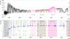 |
Fig. 1 Top panel: Q J 0643−5041 spectrum obtained after combining the 15 exposures with central grating setting at 390 nm and attached ThAr lamp exposure for wavelength calibration. In colours, the broad-line emission line intervals as expected from the composite emission spectrum of quasars from Vanden Berk et al. (2001) at zem = 3.09. Bottom panel: the median of the selected intervals from saturated Lyman-α forest absorption lines for the analysis of the zero level are shown in blue square points. The error bar on the wavelength is simply the selected interval. The error bar on the flux is the error on the mean measured flux of the selected pixels. The dashed line is the fit to the medians taking the errors into account. Green star points represent the median level at the bottom of saturated and unblended H2 lines. We compute error bars equivalent to those of blue points. We show the broad-line region expected extension as given in Vanden Berk et al. (2001) in shaded colours, and the flux measured in gray in the background. |
Summary of Q J 0643−5041 exposures containing H2 and HD absorption features at zabs≃ 2.6586, using the blue arm of the Ultraviolet and Visual Echelle Spectrograph at ESO-VLT used for analysis in the present work.
The detection of H2 at zabs= 2.66 towards Q J 0643−5041 (zem = 3.09) was first reported in Noterdaeme et al. (2008a). Several programs observed this quasar using both spectroscopic VLT-UVES arms (Dekker et al. 2000) in 2003 and 2004: 072.A-0442(A), aimed to study DLAs (PI S. López); 073.A-0071(A), aimed to search for H2-bearing systems at high redshift (PI Ledoux); and 074.A-0201(A), aimed to constrain the variation of the fine-structure constant at high redshift using metal absorption lines (PI R. Srianand). The observers used a slit of 1.2 arcsec and a 2 × 2-binned CCD, resulting in a spectral resolving power of R ~ 40 000 or full width at half maximum (FWHM) = 7.5 km s-1 in the blue arm and R ~ 36 000, or FWHM = 8.3 km s-1 in the red arm. These programs did not include attached ThAr lamp calibration exposures. We also use more recent (2007–2008) data, program ID 080.A-0228(A) aimed to constrain the cosmological variation of μ (PI Petitjean). A UVB spectrum derived from these observations is shown in Fig. 1. The settings for the exposures were a 1 arcsec slit and 2 × 2 binning of the CCD pixels, for a resolving power of R ~ 45 000, or FWHM = 6.7 km s-1 in the blue arm, and R ~ 43 000, or FWHM = 7.0 km s-1 in the red arm. We performed wavelength calibration with attached ThAr exposures. Here, we solely focused the data acquisition on H2 transitions. Hence, the H2 lines are apparent in all the observing data sets, while metal lines falling in the red arm (λ > 4500 Å) are observed only in the early observations. Blue arm exposures, relevant for detecting H2 absorption lines, are listed in Table 1.
We reduced all the data using UVES Common Pipeline Library (CPL) data reduction pipeline release 5.3.112, using the optimal extraction method. We used 4th order polynomials to find the dispersion solutions. The number of suitable ThAr lines used for wavelength calibration was usually more than 700 and the rms error was found to be in the range 70–80 m s-1 with zero average. However, this error reflects only the calibration error at the observed wavelengths of the ThAr lines that are used for wavelength calibration. Systematic errors affecting wavelength calibration should be measured with other techniques that will be discussed later in the paper. All the spectra are corrected for the motion of the observatory around the barycentre of the solar system. The velocity component of the observatory’s barycentric motion towards the line of sight to the QSO was calculated at the exposure mid point. Conversion of air to vacuum wavelengths was performed using the formula given in Edlén (1966). We interpolate these spectra into a common wavelength array and generate the weighted mean combined spectrum, using the inverse square of error as the weight. This is the combined spectrum we use to study the physical condition of this absorption system.
To study of the variation of μ, we only consider those exposures that have the attached mode ThAr lamp calibration. We follow a more careful procedure to make a new combined spectrum from these exposures. We start from the final un-rebinned extracted spectrum of each order produced by the CPL. We apply the CPL wavelength solution to each order and merge the orders by implementing a weighted mean in the overlapping regions. In the last step, we made use of a uniform wavelength array of step size of 2.0 km s-1 for all exposures. As a result, no further rebinning is required for spectrum combination. We fitted a continuum to each individual spectrum and generated a combined spectrum using a weighted mean. We further fit a lower order polynomial to adjust the continuum. This spectrum will be used for Δμ/μ measurement. In Rahmani et al. (2013), we found this procedure to produce final combined spectrum consistent with that obtained using UVES_POPLER.
3. Residual zero-level flux: partial coverage?
Quasi-stellar objects are compact objects emitting an intrinsic and extremely luminous continuum flux. Broad emission lines seen in the spectra of QSOs are believed to originate from an extended region of ~pc size, the broad-line region (BLR). Balashev et al. (2011) reported that an intervening molecular cloud towards Q1232+082 covers only a fraction of the BLR, most probably because of its compact size. This results in a residual flux detected at the bottom of saturated spectral features associated with the neutral cloud at wavelengths that are coincident with the BLR emission.
Here, we search for a similar effect. For this, we estimate the residual flux at the bottom of saturated H2 lines of the molecular cloud at zabs= 2.6586 towards Q J 0643−5041. We verify the instrumental zero flux level of the spectra first, bearing in mind that UVES is not flux calibrated. We estimate the residual flux at the bottom of saturated Lyman-α-forest lines, associated with large scale gas clouds in the intergalactic medium that are extended enough to cover the background source completely. We consider 29 sets of pixels defined by intervals in wavelengths close to the center of saturated Lyman-α-forest lines first, with no interference with H2 transitions. The median flux value for each interval with its error is represented by blue points in the bottom panel of Fig. 1. We fit the observed distribution with a simple function of the wavelength, represented by the dotted line in the bottom panel of Fig. 1, and correct the systematic zero error by subtracting it from the flux.
We estimate the residual flux at the bottom of saturated H2 transitions unblended with other absorption features. We normalise the flux and fit the H2 system. For this analysis, all fitting parameters (redshift, column density, and Doppler parameter) of a given rotational level are tied for all lines. The fit shows that for some of the most saturated lines the flux measured at the bottom of the lines is clearly above the Voigt profile absorption model. We select the pixels where the model fit falls below 1% of the emitted flux and plot in green in the bottom panel of Fig. 1 the resulting median flux of such selected pixels. The measured flux at the bottom of saturated H2 lines is systematically larger than that measured at the bottom of the Lyman-α forest saturated lines, in blue in the bottom panel in Fig. 1.
To establish whether this residual flux is due to partial coverage of the BLR, we attempt to measure the BLR emission. Unfortunately, because of the difference between emitting and absorbing redshifts, only a few saturated H2 lines fall on top of broad emission lines of C iii, N iii, Lyman-δ, and Lyman-ϵ. As shown in the top panel of Fig. 1, the relative amplitude of these features with respect to the total emitted flux is very small. Nonetheless, we estimate the Q J 0643−5041 continuum emission alone by ignoring the wavelength intervals where the BLR emission is expected as defined in Vanden Berk et al. (2001) (coloured and shaded regions in Fig. 1). After subtracting this continuum contribution, we are left with the relative BLR emission, which is plotted in solid line in Fig. 2.
In this figure, we see that green points, representing the residual flux at the bottom of H2 saturated lines, are systematically above the 1% level. Around the BLR emitting region the effect is possibly larger. Note that the variation does not follow the BLR emission fraction exactly as is also the case in Balashev et al. (2011). The distribution of these points shows roughly two behaviours. Below ~3750 Å, the points are distributed around ≃1%, and above ~3750 Å, they are distributed around ≃5%, with altogether larger dispersion towards the blue where the signal-to-noise ratio (S/N) is lower. A closer look at the distribution of these points shows that there are two distributions, one peaked at zero flux as it should be for a full absorption, and another peaked at ≃4% of the total flux. While all points, on the BLR emission lines or not, contribute to the ≃4% peak, only those not associated with BLR emission peak at zero flux. It is therefore possible that part of the BLR is not covered. The only absorption line located on top of an important broad emission line is L1R0 falling on top of C iii (see Fig. 2). It has the highest residual of all absorption lines. Actually, the residual flux matches the relative flux attributed to C iii exactly, however, this is probably a chance coincidence.
In conclusion, we can say that, although not striking, there is at least weak evidence for the BLR to be partly covered by the H2 bearing cloud (see also Sect. 5.4). A higher S/N spectrum would be required to confirm or refute the partial coverage. The effect being poorly determined and globally small, we do not attempt to take it into account when fitting H2 lines with Voigt profiles. In particular, the saturated lines we use can be fitted in the wings of the absorption profile where partial coverage does not have any impact. Moreover, metal profiles are dominated by strong and saturated components stemming from diffuse extended gas.
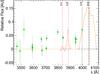 |
Fig. 2 Fraction of emitted flux attributed to the broad-line region associated with Q J 0643−5041 is drawn in solid line. We indicate the position of the emission lines at zem = 3.09. Pixels corresponding to saturated H2 transitions are shown in gray, and in green star points their median at each selected line position. |
Metal components in the absorbing system at zabs = 2.659 towards Q J 0643−5041obtained with multi-component fit using VPFIT.
4. Fit of the absorption profiles
We proceed by studying the various absorption lines associated with the DLA, fitting Voigt profiles with the Voigt profile fitting program (VPFIT) 10.03. The reference absorption redshift (defining the origin of our adopted velocity scale) is set to the position of the detected C i component, i.e., zabs = 2.65859(7).
4.1. H I content
To determine the H i absorption profile, we checked the structure of the absorption profiles of other elements thought to be associated with H i such as C ii and O i. Both of these elements feature a multi-component saturated pattern spanning about 200 km s-1 (see Fig. A.11). It is, therefore, difficult to have a precise H i absorption decomposition, hence to have a good estimate of the H i column density at the position of the molecular cloud. A main component is fixed at zabs = 2.65859(7), and the fit to Lyman-α and Lyman-β gives Nmain(H i) = 1021.03 ± 0.08 cm-2, which is consistent with all other H i transitions (see Fig. A.1). The other nine components (with Nother(H i) < 1017.3 cm-2) were added to match the H i profile down to Lyman-7.
4.2. Metal content
Low ionisation species, Fe ii, Cr ii, Si ii, Zn ii, S ii, Mg i, P ii, Cu ii, and Ni ii, are detected in a multi-component absorption pattern spanning about ~210 km s-1, with roughly a 125 km s-1 extension towards the blue and 85 km s-1 towards the red, with respect to the carbon and molecular component at z = 2.65859(7). The absorption profiles are fitted with 21 velocity components. After a first guess is obtained, we perform a fit with tied redshifts and Doppler parameters between different species. The latter is taken as the combination of a kinematical term for a fixed temperature of 104 K and a turbulent term, which is the same for all species. The resulting profile can be seen in Fig. A.11 and the parameters of the fit are given in Table 2. The turbulent term is the major component of the Doppler parameters. We caution that the Zn ii column densities over the range v = −90, −25 km s-1 are probably overestimated as they appear relatively strong compared to other species. This is likely due to contaminations from telluric features and sky line residuals. Taking the noise in the portions of spectra relevant to Zn ii into account, the 3σ detection limit is at log N ≃ 11.47, showing that the blue components of Zn ii are below the noise level. We note that using the 3σ upper-limits instead of the fitted column densities has negligible influence on the derived total column density of zinc. Interestingly, we detect weak, but significant Cu ii λ1358 absorption, consistently with non-detection of the weaker Cu ii λ1367. The profile follows that of other species well and we measure a total column density of log N(Cu ii)= 12.41 ± 0.06. To our knowledge, this is only the second detection of copper in a DLA (see Kulkarni et al. 2012).
Highly ionised species, C iv, Si iv, and Al iii, are detected with a broad profile with maximum optical depth at ~45 km s-1 towards the red from the molecular component (corresponding to components number 16 and 12 respectively, see Table 2). The latter component is quite weak compared to the strongest component. Highly ionised species are, hence, much more present redwards of the molecular component. Voigt profile fits to these elements are displayed in Fig. A.10.
4.3. Molecular hydrogen
H2, C i, and C ii⋆ column densities in the zabs = 2.6586 H2-bearing cloud towards Q J 0643−5041.
Absorption features of molecular hydrogen fall exclusively in the blue arm. We use the ThAr attached wavelength calibrated spectrum to fit the molecular transition lines with Voigt profiles.
Molecular hydrogen is detected in a single component for rotational levels J = 0 to 5. The Voigt profile fit is not always satisfactory, in particular for J = 0 and J = 1 saturated lines. As was already stated, there is often residual flux at the bottom of the saturated lines. The detection is secured for J = 0 to 5 with a reliable fit. For J = 6, the L4P6 and L5P6 are detected at the 1.7σ confidence level only. The 3σ level upper limit of the column density is N(H2, J = 6) ≤ 1013.65 cm-2. Regarding J = 7, the L5R7 is detected at the 2.1σ confidence level only. The 3σ column density upper limit is N(H2, J = 7) ≤ 1013.51cm-2. Nonetheless, we perform a fit to these rotational levels with fixed Doppler parameter (to the value of the parameter of J = 5), which is in agreement with the upper limits. A summary of the fit to the H2 lines is given in Table 3, while a selection of Voigt profile fits to the most isolated lines can be found in Figs. A.2–A.6.
The total column density is N(H2) = 1018.540 ± 0.005 cm-2 with 99% of this amount in the first two rotational levels. The molecular fraction f = 2N(H2)/(N(H i)+2N(H2)) is therefore  when taking all atomic hydrogen into account. Since the atomic hydrogen column density at the position of the molecular cloud is probably lower than the total measured column density, we get f ≳ 10-2.19. A molecular fraction of log f = −2.19 is comparable to the average molecular fractions recorded in high redshift DLA systems with log f > −4.5 (see Noterdaeme et al. 2008a) (with ten systems satisfying this condition, the mean is ⟨ log f ⟩ ≃ −2.3).
4.4. Deuterated molecular hydrogen
We study the best HD transitions available, normalising the flux locally and accounting for obvious contaminations. We select seven J = 0 transitions (L5R0, L7R0, L12R0, L13R0, W0R0, W3R0, and W4R0), and five J = 1 transitions (L2P1, L4P1, L7R1, L9P1, and W0R1). The spectral portions around these transitions are shown in Figs. A.7 and A.8 with an indicative Voigt profile model. Then we stacked these isolated spectra, weighting the transitions by the local S/N and by the oscillator strength of the transition. Finally, we compare this stack with a synthetic spectrum of the transitions with the same weights, and with redshift and Doppler parameters set to the H2J = 0, 1. The result is shown in Fig. 3. For J = 0 we clearly see a line, while for J = 1 the obtained feature seems shapeless and is dominated by unsolved contaminations. The best column densities to match the obtained spectra are N(HD, J = 0) ≃ 1013.4 ± 0.1 cm-2 and N(HD, J = 1) ≃ 1013.3 ± 0.1 cm-2. These derived column densities should be considered as upper limits, i.e, N(HD) ≲ 1013.65 ± 0.07 cm-2. A higher S/N is needed to confirm the detection.
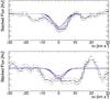 |
Fig. 3 Stacked spectra for HD J = 0 (seven lines, upper panel) and J = 1 (five lines, lower panel) transitions (solid), and the error (dotted). We also provide synthetic Voigt profile models with tied Doppler parameters and redshifts to those of H2J = 0, 1, for log N [cm-2] = 13.3, 13.4, 13.5, and log N [cm-2] = 13.2, 13.3, 13.4 respectively. |
4.5. Neutral and singly-ionised carbon
Neutral carbon is detected in a single component at a redshift close to molecules, but 250 m s-1 blueshifted. Slight differences, of the order of less than 1 km s-1 in the position of H2 and C i features have already been observed (see Srianand et al. 2012). In our case, this shift is observed over a large range of wavelengths and for several neutral carbon transitions, hence the effect is real. The absorption of C i and H2 is expected to arise in the same gas because the two species are sensitive to the same radiation, but this is only true on the first order and self-shielding effects can be subtle so that the absorption profiles can still bear small differences in shape and distribution (see, e.g., Srianand & Petitjean 1998). Therefore, it is not so surprising to observe this small 250 m s-1 shift in the centroid of the two absorbing systems.
The column densities of the three sub-levels of the ground state are respectively, N(C i)= 1012.56 ± 0.07 cm-2 for the 2s22p P
P level, N(C i⋆)= 1012.41 ± 0.14 cm-2 for the 2s22pP
 level, and Nlim(C i⋆⋆)< 1011.95 cm-2 for the 2s22pP
 level. From the measured N(C i) and N(C i⋆) column densities, and for standard conditions, we would expect the C i⋆⋆ level to have N(C i⋆⋆)≲ 1011.7 cm-2 (see Noterdaeme et al. 2007b, Fig. 8), which is consistent with the observations.
We also detected ionised carbon in the excited state C ii⋆ (2s22p 2P ) in a single well-defined component, yielding N(C ii⋆)= 1014.11 ± 0.04 cm-2, redshifted with respect to the neutral component by about 400 m s-1. We also detected C ii, however all components with Δv ≥ −30 km s-1 are strongly saturated, hence no fit could be achieved.
The results of the above fits are listed in Table 3, and the spectral features can be seen in Fig. A.9.
5. Physical characteristics of the absorption system at zabs ≃ 2.6586
5.1. Metallicity, depletion, and dust content
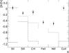 |
Fig. 4 Depletion factor, [X/Zn], of different species relative to zinc calculated by integrating the column densities over the whole profile. Dotted, dashed, and solid lines correspond to depletion factors observed in, respectively, the halo, the warm, and cold ISM of the Galaxy (Welty et al. 1999). Note that the depletion factor observed in the Galaxy for copper is unavailable. |
Integrating the column densities over all the components, we derive, [Zn/H] = −0.91 ± 0.094 and [S/H] = −0.87 ± 0.09. Again, the very good agreement between these two metallicity estimators shows that the estimated Zn ii total column density is exact. A metallicity of [X/H] ~ −0.9 is slightly high for a z ~ 2.5 DLA (Prochaska et al. 2003), to be compared to a median metallicity of ~−1.1. This supports the idea that H2 is expected to be found in relatively high-metallicity gas (Petitjean et al. 2006).
We now compare the relative abundances of elements to determine the depletion in this system. The relative amount of dust can be studied by the ratio of volatile versus refractory elements (e.g., Pettini et al. 1994). For this purpose, [S/Fe] and [Zn/Fe] are usually used (e.g., Vladilo 1998; Centurión et al. 2000), bearing in mind that sulphur is an α-element, hence its relative abundance may suffer some enhancement, and that whether zinc behaves as an α-element or an iron-peak element is not fully understood (see Rafelski et al. 2012). While Zn ii transitions are weaker and blended with Mg i and Cr ii, S ii transitions fall in the Lyman-α forest and in a portion of the spectrum where the S/N is poor. We choose to present the analysis of depletion and dust content using Zn ii, bearing in mind that the components on the blue side of the absorption profile should be taken as upper limits (see Sect. 4.2).
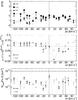 |
Fig. 5 Depletion and dust patterns through the absorption profile. Top panel: depletion of Fe, Zn, and Si with respect to S. Middle panel: dust to gas ratio computed with respect to Zn and S; the horizontal lines show the value of κ obtained when summing all components, using zinc (solid) and sulphur (dotted). Bottom panel: the iron column density in the dust phase computed with respect to Zn and S; horizontal lines mark the integrated value over all the profile, using zinc (solid) and sulphur (dotted). Vertical dashed lines show the C i and H2 component at z = 2.65859(7). |
Depletion of iron and silicon relative to zinc is mild, [Fe/Zn] = −0.45 ± 0.06 and [Si/Zn] = −0.14 ± 0.06 when summing up all components, in good agreement with [Fe/S] and [Si/S] (see Table 2). The overall depletion pattern is shown in Fig. 4 and is consistent with what is seen in the galactic halo. Copper shows no depletion: [Cu/H] = −0.88 ± 0.10, [Cu/Zn] = −0.03 ± 0.08, and [Cu/S] = −0.01 ± 0.07, similar to what was observed in the only other copper detection in a DLA system (Kulkarni et al. 2012), and in contrast to what is observed in the local ISM, with [Cu/X] ~ −1.1 in the warm ISM and [Cu/X] ~ −1.4 in the cold ISM (Cartledge et al. 2006). Note that the strictly solar relative abundances of copper, zinc, and sulphur indicates that we do not observe any α-element enrichment of zinc, contrary to what was suggested by Rafelski et al. (2012). This supports the usual interpretation that sub-solar [Fe/Zn] ratios are rather the result of iron depletion into dust grains.
It has been argued that the depletion could be larger in the components where H2 is found (see, e.g., Petitjean et al. 2002). We plot, in the top panel of Fig. 5, the depletion of S, Si, and Fe relative to Zn in each component versus the velocity position of the components with respect to the position of the C i and H2 components located at z = 2.65859(7). Notice that zinc and sulphur follow each other with mild differences on each edge of the absorption pattern. In particular, towards the blue, sulphur appears to be depleted with respect to zinc, which is unlikely to be a real effect, rather the result of the overestimation of Zn ii column densities in those components. Hence, in the following component-by-component decomposition, we must critically compare the results using zinc or sulphur as references.
We have estimated the relative dust content on a single component, or a cloud, by means of the dust to gas ratio, κ ≃ (1 − 10[Fe/X]) × 10[X/H], where X = Zn or X = S (see Prochaska et al. 2001 and Jenkins 2009). Averaging over the whole profile, we find κ ≃ 0.091 when using sulphur and κ ≃ 0.080 when using zinc, hence we estimate κ ≃ 0.08. This is a typical value for high redshift DLAs (Srianand et al. 2005b). To compute κ component by component, we will assume that the metallicity is the same for all components and equal to the DLA mean metallicity. The result is shown in the middle panel of Fig. 5.
Finally, we can also estimate the Fe ii equivalent column density trapped into dust grains in each component k:  Fe,X)= (1 − 10[Fe/X] k) Nk(X) (N(Fe)/ N(X))DLA, where (N(Fe)/ N(X))DLA is the ratio of the total column densities in the DLA and X = Zn or X = S Vladilo et al. (see 2006). The values obtained at each component are shown in the bottom panel of Fig. 5. For reference, the total values are
  Fe,Zn)≃ 1014.95 cm-2 and Fe,S)≃ 1014.97 cm-2. This system is comparable to most H2-bearing absorption systems at high redshift (Noterdaeme et al. 2008a). It is apparent from Fig. 5 that the depletion pattern is quite homogeneous through the profile, with only a mild indication for a higher dust column density at zero velocity. This indicates that the molecular component can easily be hidden in the metal profile. We note, however, that the Doppler parameter of the metal component that corresponds to H2 is significantly lower than in the rest of the profile, indicating colder gas. In addition, the profile of highly ionised species such as C iv or Si iv (Fig. A.10) is comparatively weak at the position of H2, revealing less ionisation in this component.
5.2. Thermal properties in the molecular cloud from H2 rotational level populations
H2 excitation temperatures in the zabs = 2.6586 H2-bearing cloud towards Q J 0643−5041 (all values in K).
5.2.1. Excitation temperatures
The excitation temperature Tij between two rotational levels J = i, j is defined by 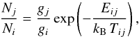 (1)where gJ is the statistical weight of the J level and Eij ≃ (j(j + 1) − i(i + 1)) × B is the energy difference between the rotational levels and B is the rotational constant of the H2 molecule (B/kB = 85.3 K). Using this relation, we compute the excitation temperatures Tij with i = 0, 3 and j = 1 ... 7. See the results in Table 4.
It is known that T01 is related to the temperature of formation on the surface of dust grains when the dominant thermalisation process is the formation of H2, and to the kinetic temperature Tkin when the dominant thermalisation process is collisions. In thick, self-shielded molecular clouds where N(H2)≥ 1016.5 cm-2, T01 is a good tracer of the kinetic temperature (see Srianand et al. 2005a; Roy et al. 2006, and references therein). Here,  K, as in most high-redshift H2-bearing clouds detected so far. Such a temperature is also very close to that of the ISM of the MW or the Magellanic Clouds, where the average temperature is found to be (77 ± 17) K (Savage et al. 1977) and (82 ± 21) K (Tumlinson et al. 2002), respectively, suggesting a cold neutral medium.
5.2.2. Ortho-para ratio and local thermal equilibrium
The ortho-para ratio (OPR), i.e., the ratio of the total population (column densities) of ortho (even J) levels to that of para (odd J) levels, is another tracer of the state of the gas in the molecular gas, and is given by  (2)Here we measure OPR = 1.06. If we assume the H2-bearing gas is at local thermal equilibrium (LTE), then we can relate the OPR to the equilibrium distribution with a single temperature for the whole gas and estimate TLTE:
 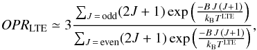 (3)where kB is the Boltzmann constant. When the kinetic temperature is high, the OPR is expected to reach a value of 3, while in cold neutral media its value is expected to be below 1 (Srianand et al. 2005a). Hence, the OPR, in agreement with the excitation temperature T01, also points towards a cold neutral medium.
 |
Fig. 6 Excitation diagram of H2. Two different behaviours are characterised by two different excitation temperatures, one for J = 0, 1, and 2 and one for J = 3, 4, and 5. The following two levels are somehow incompatible with both of these characteristic temperatures, however, the uncertainty on their column densities is too large to elaborate further. |
5.2.3. Excitation diagram
The excitation diagram, i.e., the ratio of the column density in a level to its statistical weight versus the energy difference between this level and J = 0, is presented in Fig. 6. As is shown by the two fitting lines, there seems to be two different excitation regimes, namely one for levels J = 0 ... 2 with T0J = (80.7 ± 0.8) K, and another for levels J = 3 ... 5 with  K. We limit the analysis to J = 5 since the uncertainty on the column densities of J = 6 and J = 7 is large. We can readily see that T0J, J = 1, 2 is compatible with T01. If Tij ≃ T(OPR) (≃T01), then the excitation is dominated by collisions (Srianand et al. 2005a), and this seems to be the case below J = 3. From this level and above, other mechanisms intervene, such as radiation pumping (excitation of lower levels to higher levels by UV radiation) or formation pumping (preferred formation of H2 in excited states, which then de-excite to the lower levels). From Table 4 we see that T3J is of the same order as T34 and T35.
The Doppler parameter increases with increasing rotational level. This could be the result of higher rotational levels arising mostly from the outer parts of the cloud, which are heated by photoelectric effect on dust grains by the surrounding UV flux (Ledoux et al. 2003).
5.3. Ambient UV flux
5.3.1. The UV flux from heating/cooling equilibrium
We proceed to estimate the ambient UV flux using the same procedure used by Wolfe et al. (2003). Assuming equilibrium between the photo-electric heating of the gas and the cooling by the C ii⋆ emission, together with similar interstellar medium conditions between the galaxy and DLAs (same type of dust grains, temperature, and density Weingartner & Draine 2001), we can write
  , where κ = kDLA/kMW is the relative dust to gas ratio, and kDLA and kMW are the local dust to gas ratio at the DLA and the MW and lc the cooling rate.
In the DLA we studied, we estimated the relative dust to gas ratio to be κ ≃ 0.08. Then, the average energy loss per hydrogen atom determines the cooling rate  (4)with λ(2P3/2 → 2P1/2) ≃ 158 μm and A21 ≃ 2.4 × 10⁻⁶ s-1, the wavelength and decay rate of the spontaneous photon emitting
  transition respectively (Pottasch et al. 1979; Wolfe et al. 2003). We estimate N(C ii⋆) ≃ 1014.1 cm-2 (see Table 3) and N(H i) ≃ 1021.0 cm-2. This leads to lc ≃ 10-26.4 erg s-1 per hydrogen atom. From this we derive
  .
.
5.3.2. Rotational excitation and radiation field
We estimate the ambient UV radiation, using the excitation of the high J levels, since we have seen that for J ≥ 3, the excitation temperature as deduced from the level populations is substantially larger than Tkin. Hence, these levels are excited by fluorescence, but also, the formation of H2 in high rotational levels. Following Noterdaeme et al. (2007b), formation pumping is related, at equilibrium, to the photodissociation rate such that Rform np n(H) = Rdiss n(H2), where Rform, np and Rdiss stand for the H2 formation rate, the proton density, and the H2 photodissociation rate. The latter is related to the photoabsorption rate β, which brings us to the ambient UV flux, by Rdiss = ζ β, where ζ = 0.11 is the fraction of photodissociation to photoabsorption. This yields Rform np n(H)/ n(H2)= Rdiss = ζ β. Hence, we write the equilibrium between spontaneous decay of J = 4, 5 levels (with transition probabilities A4 → 2 = 2.8 × 10⁻⁹ s-1 and A5 → 3 = 9.9 × 10⁻⁹ s-1), and UV pumping from the most populated lower levels J = 0, 1 (with efficiencies p4, 0 = 0.26 and p5, 1 = 0.12 and absorption rates β0 and β1) and formation pumping into J = 4, 5 levels (with f4 ≃ 0.19 and f5 ≃ 0.44 fractions) as  (5)and
  (6)Dividing by the H2 density, assuming the homogeneity of the gas cloud (and therefore n(H2, J)/n(H2)= N(H2, J)/N(H2)) and rearranging these equations we get
 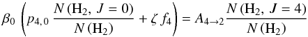 (7)and
 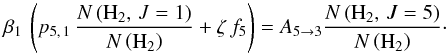 (8)Using these relations we get β0 ≃ (4.9 ± 0.2) × 10-13 s-1 and β1 ≃ (18.8 ± 1.9) × 10-13 s-1. These are extremely low values that can be explained by the shielding of the inner part of the cloud by outer layers. The large log N(H2)/ N(C i)= 5.97 ± 0.09 ratio measured in the cloud confirms, as it has already been pointed out, that large H2 column densities at high redshift, and in particular large log N(H2)/ N(C i), are associated with low photoabsorption rates (see Noterdaeme et al. 2007b, Fig. 7).
The total shielding S is the product of the molecular hydrogen self-shielding, estimated by SH2 ≃ (N(H2)/ 1014 cm by the dust extinction Sdust = exp( − τUV), and allows us to relate the photodissociation rate to JLW, the UV intensity at hν = 12.87 eV averaged over the solid angle, with the relation Rdiss = ζβ = 4π 1.1 × 10⁸ JLW S. The dust optical depth can be approximated by τUV ≃ 0.879 κ (N(H)/ 1021 cm-2) (see Noterdaeme et al. 2007a), where κ is the dust to gas ratio, as discussed in Sect. 5.1. Hence, τUV ≃ 0.07 leads to S ≃ (4 × 10-4) × (0.9) ≃ 3.8 × 10⁻⁴. Self-shielding is the dominant shielding mechanism as usual. Given this and adopting β = β0 we arrive at JLW ≃ 8 × 10-11 β0/S ≃ 8.5 × 10⁻²⁰ erg s-1 cm-2 Hz-1 sr-1, which is a factor χ = 2.6 larger than in the solar vicinity. Note that this is larger by about a factor of four compared to the value derived from the C ii⋆ absorption line. The two measurements are comparable, however, and have no a priori reason to match exactly as the C ii⋆ measurement corresponds to a mean flux in the host galaxy when the H2 measurement is related to the flux in the vicinity of the H2-bearing cloud.
Following Hirashita & Ferrara (2005), we can relate χ to the surface star forming rate ΣSFR ≃ χ × 1.7 × 10⁻³ M⊙ yr-1 kpc-2 ≃ 4.4 × 10⁻³ M⊙ yr-1 kpc-2.
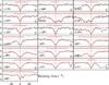 |
Fig. 7 Absorption profile of H2 transitions from the J = 1 level and the best-fitting Voigt profile. The normalised residual (i.e., ([data]−[model])/[error]) for each fit is also shown in the top of each panel along with the 1σ line. We present the clean absorption lines by putting a letter “C” in the right bottom of these transitions. |
5.4. Neutral carbon fine structure and the extension of the molecular cloud
The relative populations of the fine-structure levels of neutral carbon ground state is determined by the ambient conditions through collisions and excitation by the UV flux and the CMB radiation. We can estimate the density of the gas because for densities ≥10 cm-3 and temperatures Tkin ~ 100 K, these populations depend primarily on the hydrogen density (see Silva & Viegas 2002, Fig. 2).
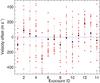 |
Fig. 8 Results of cross-correlation analysis between individual spectra and the combined one for each order. Bars present the standard deviations of the shifts measured for individual spectra. |
We measure N(C i⋆)/ N(C i)= 10− 0.10 ± 0.11 and estimate the hydrogen density to be in the range n(H)≃ (40 − 140) cm -3 with a central value of 80 cm -3 (from Noterdaeme et al. 2007b, Fig. 8).
We thus estimate the characteristic length of the cloud to be l ≃ N(H i)/ n(H): 2.3 pc ≲ l ≲ 7.9 pc. The H i column density in the main component, which bears molecules, is certainly overestimated, since species such as Fe ii, Si ii, O i, C ii, or Ni ii are found in many components spanning over 200 km s-1. Therefore, we can safely conclude that l < 8 pc. For simplicity, we assume a spherical shape, which translates into an angular size of θDLA < 0.9 mas. However, there is no reason for the length scale along the line-of-sight to be the same as the transverse extension. Moreover, the average density within the molecular cloud could be slightly different, since there is a small 250 m s-1 displacement in the centroid of the neutral carbon and H2 absorption features.
Bearing this in mind, for comparison, the angular size of a typical BLR (of extension lBLR ~ 1 pc) amounts to θBLR ~ 0.1 mas. This is fully consistent with full coverage of the BLR by the DLA. Nonetheless, the size of the molecular cloud could be much smaller. Balashev et al. (2011) estimated that the molecular cloud at z = 2.34 towards Q1232+082 has an extension of (0.15 ± 0.05) pc, hence it could well be two orders of magnitude smaller than 0.9 mas. Given this, it is impossible to conclude the actuality of the partial coverage of the BLR by the H2-bearing cloud.
Δμ/μ estimations using H2 lines in the zabs = 2.6586 H2-bearing cloud towards Q J 0643−5041.
6. Constraints to the cosmic variation of the proton-to-electron mass ratio with Q J 0643−5041
In the case of H2 molecule, the energy difference between rotational states and vibrational states is proportional to the reduced mass of the system and its square root, respectively. Using intervening molecular absorption lines seen in the high-z quasar spectra for measuring Δμ/μ (i.e., Δμ/μ ≡ (μz − μ0)/μ0 where μz and μ0 are the values of proton-to-electron mass ratio at redshift z and today) in the distant universe was first proposed by Thompson (1975).
The sensitivity of the wavelength of the i’th H2 transition to the variation of μ is generally parametrised as  (9)where
  is the rest frame wavelength of the transition, λi is the observed wavelength, Ki is the sensitivity coefficient of i’th transition, given by
  , and zabs is the redshift of the H2 system. Here we use the most recent data on Ki given by Meshkov et al. (2006), Ubachs et al. (2007) and the rest wavelengths and oscillator strengths from Malec et al. (2010). Equation (9) can be rearranged as
 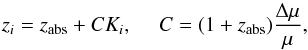 (10)which clearly shows that zabs is only the mean redshift of transitions with Ki = 0. The redshift of the i’th H2 transition is denoted by zi. The expression in Eq. (10) is sometimes presented as
  (11)which shows the value of Δμ/μ can be determined, using the reduced redshift (zred) versus Ki. At present, measurements of Δμ/μ, using H2 at z ≥ 2, are limited to six H2-bearing DLAs (see Varshalovich & Levshakov 1993; Cowie & Songaila 1995; Levshakov et al. 2002; Ivanchik et al. 2005; Reinhold et al. 2006; Ubachs et al. 2007; Thompson et al. 2009; Wendt & Molaro 2011, 2012; Rahmani et al. 2013). All these measurements are consistent with Δμ/μ being zero at the level of 10 ppm. Here we present a new Δμ/μ constraint, using the zabs= 2.6586 absorbing system towards Q J 0643−5041.
Like in Rahmani et al. (2013) we use two approaches to measure Δμ/μ. In the first approach, we fit the H2 lines, using a single velocity component, and estimate the redshift for each H2 transitions, and measure Δμ/μ using Eq. (11). In the second approach, we explicitly use Δμ/μ as one of the fitting parameters in addition to N, b, and z in VPFIT. This approach allows for a multi-component fit of the H2 lines. The results of Δμ/μ for various approaches are given in Table 5.
To carry out a measurement of μ, we need to choose a suitable set of H2 lines. Although H2 absorption from high J-levels (J = 4–7) is detected towards Q J 0643−5041, it is are too weak to lead to very accurate redshift measurements, as required for this study. Therefore, we reject H2 lines from these high-J levels while measuring Δμ/μ, and only use H2 absorption features from J = 0–3. By carefully inspecting the combined spectrum, we identified 81 lines suitable for Δμ/μ measurements. A list of H2 transitions we used is tabulated in Table B.1, where clean lines are highlighted. Thirty-eight out of 81 lines are mildly blended with the intervening Lyman-α absorption of the intergalactic medium. We accurately model surrounding contaminations using multi-component Voigt-profile fitting, while simultaneously fitting the H2 lines (see Fig. 7).
6.1. Systematic wavelength shifts: cross-correlation analysis
D’Odorico et al. (2000) have shown that the resetting of the grating between an object exposure and the ThAr calibration lamp exposure can result in an error of the order of a few hundred meters per second in the wavelength calibration. To minimise the errors introduced via such systematics in our Δμ/μ measurements, we do not use those exposures without attached mode ThAr calibration lamps. We further exclude the exposure with 1389 s of EXPTIME (10th row of Table 1) as the quality of this spectrum is very poor. Therefore, the combined spectrum to be used for measuring Δμ/μ is made of 14 exposures with S/N of between 11–31 over our wavelength range of interest.
The shortcomings of the ThAr calibration of VLT/UVES spectra have been shown by a number of authors (Chand et al. 2006; Levshakov et al. 2006; Molaro et al. 2008; Thompson et al. 2009; Whitmore et al. 2010; Agafonova et al. 2011; Wendt & Molaro 2011; Rahmani et al. 2012, 2013; Agafonova et al. 2013). Here we carry out a cross-correlation analysis between the combined spectrum and the individual exposures to estimate the offset between them over the wavelength range of echelle orders of the blue arm. To do so we rebin each pixel of size 2.0 km s-1 into 20 sub-pixels of size 100 m s-1 and measure the offset as corresponding to the minimum value of the χ2 estimator of the flux differences in each window (see Rahmani et al. 2013, for more detail). Each cross-correlating window spans an echelle order. The accuracy of this method is well demonstrated via a Monte Carlo simulation analysis in Rahmani et al. (2013). Figure 8 shows the results of such cross-correlation analysis.
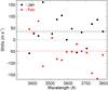 |
Fig. 9 Cross-correlation analysis between the combined spectrum of the exposures taken in early January and combined spectrum of those in February. |
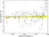 |
Fig. 10 Reduced redshift vs. the Ki for the fit with different b for different J-levels. Different J-levels are plotted with different symbols. The best-fitting linear line is also shown. The yellow region shows the 1σ error in the fitted line. |
We observe that EXP5 has the maximum constant offset of − 287 m s-1, while other exposures show constant offsets consistent with zero shift. We correct the measured shifts for individual orders of each exposure and make a new combined spectrum, and subsequently analyse its impact on Δμ/μ.
To check the stability of the spectra over a one-month period of observations, we make two combined spectra of EXP7 – EXP14 and EXP17 – EXP20. Fig. 9 shows the results of cross-correlation of these two spectra with the combined spectrum. The first three circle-asterisks pairs at λ < 3450 Å and the pair at 3650 Å present an opposite trend in comparison to the rest of the pairs. However, apart from a constant shift of ~80 m s-1, there is not any strong evidence for the existence of possible wavelength dependent systematics.
Furthermore, Rahmani et al. (2013) compared the asteroids spectra from UVES and the solar spectrum to discover a wavelength dependent systematic error in UVES observations. Moreover, they showed that such systematic errors can mimic a Δμ/μ in the range of 2.5–13.7 ppm, which changes in different epochs from 2010 to 2012. Such a systematic error cannot be revealed from the cross-correlation analysis between the individual exposures and the combined spectrum of this quasar, i.e., without a reference spectrum. Unfortunately, we do not have asteroid observations with the same settings of and close in time to our science observations, hence we are not in a position to check whether such a drift is present in our data. Ceres has been observed with the 346 setting of UVES on 05-12-2007 and without attached mode ThAr lamp. However, such an observation is not an appropriate reference to study the effect of a wavelength drift in 390 setting observations, hence we have not corrected the data using this drift measurement.
6.2. Limits on Δμ/μ at z = 2.6586: first approach
Most measurements of Δμ/μ using H2 use the measured slope between the reduced redshifts and Ki. The most important step in this approach is to measure the redshifts and the associated errors of a set of chosen H2 absorption lines.
To measure the redshifts of the suitable H2 lines, first we choose a model in which all the J-levels have the same b parameter. The best-fitting model in this case has a reduced χ2 ( ) of 1.57. Inspecting the spectrum and the normalised residual (([data]–[model])/[error]) of the best-fitting model show that the relatively large is mainly due to the underestimation of the flux error and not due to a poor Voigt profile model. A z-vs.-K analysis of the fitted redshifts based on a linear regression yields Δμ/μ = (5.0 ± 6.1) ppm. The quoted error is obtained using the bootstrap technique. Indeed, we generate 2000 random realizations of the measured redshifts and estimate Δμ/μ for each realization. We finally quote the 1σ scatter of the 2000 Δμ/μ thus obtained as the estimated error.
The physical conditions in this H2 system and also other H2 systems (see Noterdaeme et al. 2007a) shows that different J-levels may bear different turbulent broadening parameters. In particular, J = 0 and 1 have smaller b-parameters compared to higher J-levels. Hence we define a second model in which different J-levels are allowed to have different b-parameters. The best such fitted model has a = 1.55. The z-vs.-K analysis out of these fitted redshifts yields Δμ/μ = (4.6 ± 5.9) ppm, which is very much consistent with the value obtained with the first model. Figure 10 presents the results of this fit.
Applying the above discussed models on the shift-corrected combined spectrum, we find Δμ/μ of (8.1 ± 6.6) ppm and (7.6 ± 6.4) ppm for tied and untied b, respectively. While consistent, both values are ~3 ppm larger in comparison with the uncorrected values.
6.3. Limits on Δμ/μ at z = 2.6586 directly from VPFIT
Next, we include Δμ/μ as a parameter of the fits. Using a single component model and assuming the fitted b parameter value to be the same for all J-levels, the best fit converges to Δμ/μ = (4.8 ± 4.2) ppm with an overall reduced χ2 of 1.60. The quoted error of 4.2 ppm in Δμ/μ is already scaled with  . We implement similar scaling of the statistical errors each time we find
  . This result is very much consistent with the previous findings. We apply the same analysis to the combined spectrum made of CPL generated 1-d spectra. For this model, we find Δμ/μ = (9.1 ± 4.7) ppm for such a combined spectrum. The two values differ by ~1σ. Therefore, systematic errors as large as 4.3 ppm can be produced if we use the final 1-d spectra generated by CPL.
In the last column of Table 5, we provide the Akaike information criteria (AIC; Akaike 1974) corrected for the finite sample size (AICC; Sugiura 1978) as given in Eq. (4) of King et al. (2011). While the Δμ/μ error from the bootstrap is sensitive to the redshift distribution of H2 lines, the VPFIT errors purely reflect the statistical errors. Hence, the larger error from the bootstrap method can be used to quantify the associated systematic errors. If we quadratically add 4.4 ppm to the VPFIT error, which is 4.2 ppm, we get the bootstrap error. Therefore, we can associate a systematic error to each VPFIT measurement by comparing the VPFIT error with the bootstrap error.
In the fourth line of Table 5, we present the results of the fit when b parameters in different J-levels are allowed to be different. While the best-fitting Δμ/μ of (5.5 ± 4.3) ppm is consistent with the case when we use a common b value for all J-levels, the AICC value is slightly better. In this case, the comparison of the estimated error from the bootstrap method (second line in Table 5) suggests a systematic error of 4.0 ppm.
We also consider two velocity component models. The two-component fit with common b for different J levels systematically drops one of the components while minimizing the χ2. However, when the Doppler parameter is different for different J-levels we are able to obtain a consistent two-component fit. The two components are separated by (0.19 ± 0.11) km s-1. We find Δμ/μ = (6.5 ± 4.3) ppm for such a fit. The results are summarised in the last row of Table 5. We also present the two-component fit results using shift-corrected data in Table 5. The values of Δμ/μ are larger by ~2–3 ppm for all of the models after correcting the spectra for the shifts. It is clear that while there is a marginal improvement in the and AICC the final results are very much consistent with one another. Moreover, we see that the best model is the two-component model for both shift-corrected and not corrected spectra, based on the data in Table 5. Therefore, we choose the two-component H2 fit as the best model of the data. As in Rahmani et al. (2013) we quote the final error in Δμ/μ including the systematic error obtained above and the statistical error given by VPFIT. Therefore, we consider the best-fitting measurement to be Δμ/μ = (7.4 ± 4.3stat ± 5.1sys) ppm.
7. Conclusions and discussion
We have studied the physical properties of the molecular hydrogen gas associated with the DLA system at zabs = 2.6586 towards the high redshift (zem = 3.09) quasar Q J 0643−5041, using VLT-UVES data with a total integration time of 23 h.
We find that the DLA (log N(H i)(cm-2) = 21.03 ± 0.08) has typical characteristics of the high-redshift DLA population associated with molecular clouds, with metallicity [Zn/H] = −0.91 ± 0.09 and depletion of iron relative to zinc [Zn/Fe] = 0.45 ± 0.06, and a hydrogen molecular fraction of log f =  . Molecular hydrogen is detected up to J = 7 and the excitation diagram exhibits two temperatures, T = 80.7 ± 0.8 and 551 ± 40 K for J < 3 and >3, respectively. The ambient UV radiation field, derived from the C iiλ156μ radiation, and from the analysis of the H2 UV pumping, is of the order of the MW field.
We study the possibility that the H2 bearing cloud does not cover the background source completely. For this, we analyse the distribution of residual flux observed at the bottom of saturated H2 lines and estimate the relative contributions from the BLR and AGN continuum to the emitted flux. We find that there is weak evidence for a possible excess of residual light from the BLR. Given the density derived from the C i absorption lines (nH in the range 40−140 cm-3) and the H i column density, we derive a dimension of the cloud of the order of 2.5−8 pc. This is consistent with the fact that the residual flux, if real, is small and the cloud covers most of the BLR.
We have attempted to measure HD at the same redshift as H2. By stacking the best defined features, we have been able to set an upper limit of N(HD)≲ 1013.65 ± 0.07cm-2. Deuterium is formed in the primordial universe and is subsequently progressively destroyed in stars. Therefore, one expects the abundance of deuterium to be at most equal to the primordial value, stemming from primordial nucleosynthesis, in most metal poor gas, and smaller if its local destruction is already onset. In molecular clouds, deuterated molecular hydrogen is expected to form along with H2 in shielded environments. In high redshift quasar absorption lines, only six detections have been reported so far: towards Q1232+082 (Varshalovich et al. 2001; Ivanchik et al. 2010); towards Q143912.04+111740.4 (Srianand et al. 2008; Noterdaeme et al. 2008b); towards J0812+3208 and Q1331+170 (Balashev et al. 2010); towards J123714.60+064759.5 (Noterdaeme et al. 2010); and towards J21230500 (Tumlinson et al. 2010). When HD is detected, it is possible to probe the deuterium abundance by studying the N(HD)/ 2N(H2) ratio, which should be a lower limit for D/H. A smaller deuterium fraction in molecules would be the consequence of differences in chemical molecular formation processes and of differential photo-dissociation (see, e.g., Tumlinson et al. 2010). All observations up to now seem to show that the measured HD/2H2 ratio is surprisingly high (Balashev et al. 2010; Ivanchik et al. 2010), with typical values of fD between − 4.8 and − 4.4 (Tumlinson et al. 2010). The D fraction, fD ≃ N(HD)/ 2N(H2), in this system is then ≲(6.50 ± 1.07) × 10-6 = 10− 5.19 ± 0.07, to be compared to the primordial abundance of deuterium, which is of log D/H = − 4.60. Hence, in the cloud at zabs= 2.6586 towards Q J 0643−5041, the relative deuterium abundance is half an order of magnitude lower than the primordial value. This value can also be compared to what is seen in the Milky Way. Lacour et al. (2005) find that fD increases with increasing molecular fraction. Extrapolating towards the molecular fraction of f = − 2.19 would yield fD ≃ − 7.5, which is two orders of magnitude below the upper limit we determine. Large HD/2H2 ratios seem to be common at high redshift and remain unexplained (see Tumlinson et al. 2010).
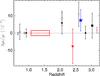 |
Fig. 11 Comparison of Δμ/μ measurement in this work and those in the literature. All measurements at 2.0 < z < 3.1 are based on the analysis of H2 absorption. The filled larger blue star shows our result and the smaller red star shows the result from Rahmani et al. (2013). The downwards empty and filled triangles are the Δμ/μ measurements from van Weerdenburg et al. (2011) and Malec et al. (2010). The filled upward triangle and the empty and filled squares are, respectively, from King et al. (2008; 2011), and Wendt & Molaro (2012). The solid box and the open circle present the constraint obtained, respectively, by Rahmani et al. (2012) and Srianand et al. (2010) based on the comparison between 21-cm and metal lines in Mg ii absorbers under the assumption that α and gp have not varied. The Δμ/μ at z < 1 are based on ammonia and methanol inversion transitions: their 5σ errors are shown. The two measurements at z ~ 0.89 with larger and smaller errors are, respectively, from Henkel et al. (2009) and Bagdonaite et al. (2013) based on the same system. The two Δμ/μ at z ~ 0.684 with larger and smaller errors are, respectively, from Murphy et al. (2008) and Kanekar (2011) based on the same system. |
We take fourteen ~1 h exposures with attached ThAr calibrations to reduce systematics in the wavelength calibration. We used this data to constrain the variation of the μ at the redshift of the DLA. We selected 81 H2 lines suitable for Δμ/μ measurements. We find that the two-velocity component model with untied Doppler parameters between different rotational levels can best model the absorption profiles of H2 lines of this system. We measure Δμ/μ = (7.4 ± 4.3stat ± 5.1sys) ppm for such a model. Our result is consistent with no variation of μ over the last 11.2 Gyr. If we add the systematic and statistical errors quadratically, we get the total error of 6.7 ppm in our Δμ/μ measurement. This is ~30% smaller than the error (10.1 ppm) in Δμ/μ, which we have obtained in a recent study of an H2 system towards HE 0027−1836 at zabs = 2.4018 (Rahmani et al. 2013). The main reason for the smaller error in the current study is the wider Ki range covered by the H2 lines towards Q J 0643−5041 compared to those of HE 0027−1836. This is an important consideration that should be taken into account in selection of systems for the study of Δμ/μ.
Figure 11 summarises Δμ/μ measurements based on different approaches at different redshifts. Our new measurement is consistent with all the other measurements based on H2 lines. However, we also note that like the majority of other studies, our Δμ/μ is positive although consistent with zero.
King et al. (2011) and van Weerdenburg et al. (2011) used H2 and HD absorbers at z = 2.811 and 2.059 towards Q0528−250 and J2123−005 respectively, to find Δμ/μ = (0.3 ± 3.2stat ± 1.9sys) × 10-6 and Δμ/μ = (8.5 ± 4.2) × 10-6. Wendt & Molaro (2012) and Rahmani et al. (2013) found Δμ/μ = (4.3 ± 7.2) × 10-6 and Δμ/μ = −(7.6 ± 10.2) × 10-6, using the H2 absorber at z = 3.025 and 2.4018 towards Q0347−383 and HE 0027−1836.
King et al. (2008) find Δμ/μ = (10.9 ± 7.1) × 10-6 at z = 2.595 towards Q0405−443. The weighted mean of these measurements and ours is of Δμ/μ = (4.5 ± 2.2) × 10-6. Wavelength dependent drifts, recently reported in UVES observations, can bias the Δμ/μ values to positive values. Therefore, caution should be exercised while interpreting such results as whole.
The best constraints on Δμ/μ have been achieved by using NH3 or CH3OH absorption lines (Murphy et al. 2008; Henkel et al. 2009; Kanekar 2011; Bagdonaite et al. 2013). Very high sensitivity of the inversion transitions associated with these molecules to Δμ/μ leads to constraint of the order of 10-7. The main drawback of this method is that only two systems at z < 1 provide the opportunity to carry out such measurements. Based on 21 cm absorption we found Δμ/μ = 0.0 ± 1.5 ppm, at z ~ 1.3 by Rahmani et al. (2012), and − (1.7 ± 1.7) ppm, at z ~ 3.2 by Srianand et al. (2010). While these measurements are more stringent than those based on H2, we need to assume no variation of α and gp to get a constraint on Δμ/μ, which is not the case in high redshift H2 absorption systems.
A further cumulation of data on the line of sight of Q J 0643−5041 would allow us to establish the actuality of partial coverage of the BLR by the H2-bearing cloud as well as the possible detection of HD. However, it seems rather difficult to go much beyond our analysis on the variation of μ with UVES data. Indeed, systematic drifts in wavelength calibration over the whole blue arm of UVES can only be unveiled by absolute reference observations (of asteroids or an iodine cell, for example) in the same conditions as science observations to correct for instrumental misbehaviours. Such a systematic effect could be the origin of the preferred positive value of Δμ/μ seen in this and other similar works. To shed light on the actual value of μ at high redshift, it is crucial to re-observe systems, such as the one presented here, with as much control in wavelength calibration as possible to account for systematics that escape our means in the present state of the art.
Online material
Appendix A: Spectral features
We present here the spectrum bits containing some of the absorption features that were fitted for the system at zabs ≃ 2.6586. Figure A.1 shows the H i absorption with the statistical error associated with the fit represented by the shaded region. Figures A.2–A.6 show the H2 lines ordered by J-level. Figures A.7 and A.8 show the attempt to fit HD absorptions. The results of this fit are possibly overestimating the column density and Doppler parameter. Figure A.9 shows the low-ionisation carbon features. In Fig. A.11, we present low ionisation metal absorption profiles, while Fig. A.10 shows highly ionised carbon and silicon lines.
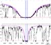 |
Fig. A.1 Voigt profile fits to the DLA: Lyman-α transition on top, Lyman-β at lower panel. The fit to the data with its uncertainty is shown in the shaded area. Vertical dashed lines mark the position of the H i components used for the fit, determined both from the wings of Lyman-α and Lyman-β and the profile of higher Lyman transitions. The observational error is shown at the bottom for reference. |
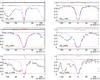 |
Fig. A.2 Voigt profile fits to H2J = 0. The fit to the data is represented by a line. Residuals of the fit are shown on top. The observational error is shown at the bottom for reference. Presence of residual flux is obvious in a few cases. |
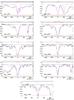 |
Fig. A.3 Voigt profile fits to H2J = 1. The fit to the data is represented by a line. Residuals of the fit are shown on top. The observational error is shown at the bottom for reference. |
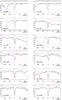 |
Fig. A.4 Voigt profile fits to H2J = 2. The fit to the data is represented by a line. Residuals of the fit are shown on top. The observational error is shown at the bottom for reference. |
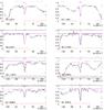 |
Fig. A.5 Voigt profile fits to H2J = 3. The fit to the data is represented by a line. Residuals of the fit are shown on top. The observational error is shown at the bottom for reference. |
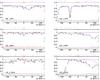 |
Fig. A.6 Voigt profile fits to H2J = 4 and 5. The fit to the data is represented by a line. Residuals of the fit are shown on top. The observational error is shown at the bottom for reference. |
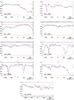 |
Fig. A.7 Selection of HD J = 0 absorption features. A tentative fit to the data is represented by a line for reference. Residuals of the fit are shown on top. The observational error is shown at the bottom for reference. |
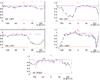 |
Fig. A.8 Selection of HD J = 1 absorption features. A tentative fit to the data is represented by a line for reference. Residuals of the fit are shown on top. The observational error is shown at the bottom for reference. |
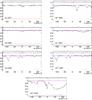 |
Fig. A.9 Voigt profile fits to carbon features. The fit to the data is represented by a line. Residuals of the fit are shown on top. The observational error is shown at the bottom for reference. |
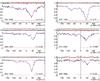 |
Fig. A.10 Multiple-component Voigt profile fits to high ionisation element profiles. The fit to the data is represented by a line. Residuals of the fit are shown in red on top when corresponding to the intervals used for the fit, and otherwise in black. The observational error is shown at the bottom for reference. |
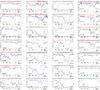 |
Fig. A.11 Multiple-component Voigt profile fits to low ionisation element profiles. The fit to the data is represented by a line. Residuals of the fit are shown on top, in red when corresponding to the intervals used for the fit, in black otherwise. The observational error is shown at the bottom for reference. C ii and O i are impossible to decompose because all features are heavily saturated. |
Appendix B: Transitions used for Δμ/μ and their redshifts
We summarise in Table B.1 the H2 lines used for the determination of Δμ/μ. We present the rest frame wavelength and sensitivity coefficients we used, the redshifts we have measured with a two-component model and Δμ/μ included as a free parameter of the fit, as well as the velocity shift with respect to the H2-bearing cloud redshift.
Laboratory wavelength of the set of H2 transitions that are fitted along with the best redshift and errors from Vogit profile analysis. The uncontaminated (CLEAN) H2 lines are highlighted in bold letters.
In the laboratory: μlab = mp/me ≃ 1836.1526675(39) (Mohr & Taylor 2000).
By definition [X/Y] ≡ log [N(X)/ N(Y)] − log [N(X)/ N(Y)] ⊙ where all solar values are taken from Lodders (2003).
Acknowledgments
This research was supported by the Agence Nationale pour la Recherche under Prog. ANR-10-BLAN-510-01. R.S. and P.P.J. gratefully acknowledge support from the Indo-French Centre for the Promotion of Advanced Research (Centre Franco-Indien pour la Promotion de la Recherche Avancée) under contract No. 4304-2. H.R. would like to thank the Institute for research in Fundamental Sciences (IPM, Tehran) for hospitality and providing facilities during his visit in August 2013. The authors would like to thank the referee, Paolo Molaro, for useful comments and discussion.
References
- Agafonova, I. I., Molaro, P., Levshakov, S. A., & Hou, J. L. 2011, A&A, 529, A28 [NASA ADS] [CrossRef] [EDP Sciences] [Google Scholar]
- Agafonova, I. I., Levshakov, S. A., Reimers, D., Hagen, H.-J., & Tytler, D. 2013, A&A, 552, A83 [NASA ADS] [CrossRef] [EDP Sciences] [Google Scholar]
- Akaike, A. 1974, IEEE Trans. Autom. Control, 19, 716 [NASA ADS] [CrossRef] [MathSciNet] [Google Scholar]
- Bagdonaite, J., Jansen, P., Henkel, C., et al. 2013, Science, 339, 46 [NASA ADS] [CrossRef] [Google Scholar]
- Balashev, S. A., Ivanchik, A. V., & Varshalovich, D. A. 2010, Astron. Lett., 36, 761 [NASA ADS] [CrossRef] [Google Scholar]
- Balashev, S., Petitjean, P., Ivanchik, A., et al. 2011, MNRAS, 418, 357 [NASA ADS] [CrossRef] [EDP Sciences] [PubMed] [Google Scholar]
- Carswell, R. F., Becker, G. D., Jorgenson, R. A., Murphy, M. T., & Wolfe, A. M. 2012, MNRAS, 422, 1700 [NASA ADS] [CrossRef] [Google Scholar]
- Cartledge, S. I. B., Lauroesch, J. T., Meyer, D. M., & Sofia, U. J. 2006, ApJ, 641, 327 [NASA ADS] [CrossRef] [Google Scholar]
- Centurión, M., Bonifacio, P., Molaro, P., & Vladilo, G. 2000, ApJ, 536, 540 [NASA ADS] [CrossRef] [Google Scholar]
- Chand, H., Srianand, R., Petitjean, P., et al. 2006, A&A, 451, 45 [NASA ADS] [CrossRef] [EDP Sciences] [Google Scholar]
- Cowie, L. L., & Songaila, A. 1995, ApJ, 453, 596 [NASA ADS] [CrossRef] [Google Scholar]
- Cui, J., Bechtold, J., Ge, J., & Meyer, D. M. 2005, ApJ, 633, 649 [Google Scholar]
- Dekker, H., D’Odorico, S., Kaufer, A., Delabre, B., & Kotzlowski, H. 2000, in SPIE Conf. Ser. 4008, eds. M. Iye, & A. F. Moorwood, 534 [Google Scholar]
- D’Odorico, S., Cristiani, S., Dekker, H., et al. 2000, in SPIE Conf. Ser. 4005, ed. J. Bergeron, 121 [Google Scholar]
- Edlén, B. 1966, Metrologia, 2, 71 [NASA ADS] [CrossRef] [Google Scholar]
- Fynbo, J. P. U., Ledoux, C., Noterdaeme, P., et al. 2011, MNRAS, 413, 2481 [NASA ADS] [CrossRef] [Google Scholar]
- Guimarães, R., Noterdaeme, P., Petitjean, P., et al. 2012, AJ, 143, 147 [NASA ADS] [CrossRef] [Google Scholar]
- Henkel, C., Menten, K. M., Murphy, M. T., et al. 2009, A&A, 500, 725 [NASA ADS] [CrossRef] [EDP Sciences] [Google Scholar]
- Hirashita, H., & Ferrara, A. 2005, MNRAS, 356, 1529 [NASA ADS] [CrossRef] [Google Scholar]
- Ivanchik, A., Petitjean, P., Varshalovich, D., et al. 2005, A&A, 440, 45 [NASA ADS] [CrossRef] [EDP Sciences] [Google Scholar]
- Ivanchik, A. V., Petitjean, P., Balashev, S. A., et al. 2010, MNRAS, 404, 1583 [NASA ADS] [Google Scholar]
- Jenkins, E. B. 2009, ApJ, 700, 1299 [NASA ADS] [CrossRef] [Google Scholar]
- Jorgenson, R. A., Wolfe, A. M., & Prochaska, J. X. 2010, ApJ, 722, 460 [NASA ADS] [CrossRef] [Google Scholar]
- Kanekar, N. 2011, ApJ, 728, L12 [NASA ADS] [CrossRef] [Google Scholar]
- King, J. A., Webb, J. K., Murphy, M. T., & Carswell, R. F. 2008, Phys. Rev. Lett., 101, 251304 [NASA ADS] [CrossRef] [PubMed] [Google Scholar]
- King, J. A., Murphy, M. T., Ubachs, W., & Webb, J. K. 2011, MNRAS, 417, 3010 [NASA ADS] [CrossRef] [Google Scholar]
- Kulkarni, V. P., Meiring, J., Som, D., et al. 2012, ApJ, 749, 176 [NASA ADS] [CrossRef] [Google Scholar]
- Lacour, S., André, M. K., Sonnentrucker, P., et al. 2005, A&A, 430, 967 [NASA ADS] [CrossRef] [EDP Sciences] [Google Scholar]
- Ledoux, C., Petitjean, P., & Srianand, R. 2003, MNRAS, 346, 209 [NASA ADS] [CrossRef] [Google Scholar]
- Levshakov, S. A., Dessauges-Zavadsky, M., D’Odorico, S., & Molaro, P. 2002, MNRAS, 333, 373 [NASA ADS] [CrossRef] [Google Scholar]
- Levshakov, S. A., Centurión, M., Molaro, P., et al. 2006, A&A, 449, 879 [NASA ADS] [CrossRef] [EDP Sciences] [Google Scholar]
- Lodders, K. 2003, ApJ, 591, 1220 [NASA ADS] [CrossRef] [Google Scholar]
- Malec, A. L., Buning, R., Murphy, M. T., et al. 2010, MNRAS, 403, 1541 [NASA ADS] [CrossRef] [Google Scholar]
- Meshkov, V., Stolyarov, A., Ivanchik, A., & Varshalovich, D. 2006, J. Exp. Theoret. Phys. Lett., 83, 303 [Google Scholar]
- Mohr, P., & Taylor, B. 2000, Rev. Mod. Phys., 72, 351 [NASA ADS] [CrossRef] [Google Scholar]
- Molaro, P., Levshakov, S. A., Monai, S., et al. 2008, A&A, 481, 559 [NASA ADS] [CrossRef] [EDP Sciences] [Google Scholar]
- Murphy, M. T., Flambaum, V. V., Muller, S., & Henkel, C. 2008, Science, 320, 1611 [NASA ADS] [CrossRef] [PubMed] [Google Scholar]
- Noterdaeme, P., Ledoux, C., Petitjean, P., et al. 2007a, A&A, 474, 393 [Google Scholar]
- Noterdaeme, P., Petitjean, P., Srianand, R., Ledoux, C., & Le Petit, F. 2007b, A&A, 469, 425 [NASA ADS] [CrossRef] [EDP Sciences] [Google Scholar]
- Noterdaeme, P., Ledoux, C., Petitjean, P., & Srianand, R. 2008a, A&A, 481, 327 [NASA ADS] [CrossRef] [EDP Sciences] [Google Scholar]
- Noterdaeme, P., Petitjean, P., Ledoux, C., Srianand, R., & Ivanchik, A. 2008b, A&A, 491, 397 [NASA ADS] [CrossRef] [EDP Sciences] [Google Scholar]
- Noterdaeme, P., Petitjean, P., Ledoux, C., et al. 2010, A&A, 523, A80 [NASA ADS] [CrossRef] [EDP Sciences] [Google Scholar]
- Noterdaeme, P., López, S., Dumont, V., et al. 2012, A&A, 542, L33 [NASA ADS] [CrossRef] [EDP Sciences] [Google Scholar]
- Petitjean, P., Srianand, R., & Ledoux, C. 2000, A&A, 364, L26 [NASA ADS] [Google Scholar]
- Petitjean, P., Srianand, R., & Ledoux, C. 2002, MNRAS, 332, 383 [NASA ADS] [CrossRef] [Google Scholar]
- Petitjean, P., Ledoux, C., Noterdaeme, P., & Srianand, R. 2006, A&A, 456, L9 [NASA ADS] [CrossRef] [EDP Sciences] [Google Scholar]
- Pettini, M., Smith, L. J., Hunstead, R. W., & King, D. L. 1994, ApJ, 426, 79 [NASA ADS] [CrossRef] [Google Scholar]
- Pettini, M., Smith, L. J., King, D. L., & Hunstead, R. W. 1997, ApJ, 486, 665 [NASA ADS] [CrossRef] [Google Scholar]
- Pottasch, S. R., Wesselius, P. R., & van Duinen, R. J. 1979, A&A, 74, L15 [NASA ADS] [Google Scholar]
- Prochaska, J. X., Gawiser, E., & Wolfe, A. M. 2001, ApJ, 552, 99 [NASA ADS] [CrossRef] [Google Scholar]
- Prochaska, J. X., Gawiser, E., Wolfe, A. M., Castro, S., & Djorgovski, S. G. 2003, ApJ, 595, L9 [NASA ADS] [CrossRef] [Google Scholar]
- Rafelski, M., Wolfe, A. M., Prochaska, J. X., Neeleman, M., & Mendez, A. J. 2012, ApJ, 755, 89 [NASA ADS] [CrossRef] [Google Scholar]
- Rahmani, H., Srianand, R., Gupta, N., et al. 2012, MNRAS, 425, 556 [NASA ADS] [CrossRef] [Google Scholar]
- Rahmani, H., Wendt, M., Srianand, R., et al. 2013, MNRAS, 435, 861 [NASA ADS] [CrossRef] [Google Scholar]
- Reinhold, E., Buning, R., Hollenstein, U., et al. 2006, Phys. Rev. Lett., 96, 151101 [NASA ADS] [CrossRef] [Google Scholar]
- Roy, N., Chengalur, J. N., & Srianand, R. 2006, MNRAS, 365, L1 [NASA ADS] [CrossRef] [Google Scholar]
- Savage, B. D., Bohlin, R. C., Drake, J. F., & Budich, W. 1977, ApJ, 216, 291 [NASA ADS] [CrossRef] [Google Scholar]
- Silva, A. I., & Viegas, S. M. 2002, MNRAS, 329, 135 [NASA ADS] [CrossRef] [Google Scholar]
- Srianand, R., & Petitjean, P. 1998, A&A, 335, 33 [NASA ADS] [Google Scholar]
- Srianand, R., Petitjean, P., Ledoux, C., Ferland, G., & Shaw, G. 2005a, MNRAS, 362, 549 [Google Scholar]
- Srianand, R., Shaw, G., Ferland, G., Petitjean, P., & Ledoux, C. 2005b [arXiv:astro-ph/0506556] [Google Scholar]
- Srianand, R., Noterdaeme, P., Ledoux, C., & Petitjean, P. 2008, A&A, 482, L39 [NASA ADS] [CrossRef] [EDP Sciences] [Google Scholar]
- Srianand, R., Gupta, N., Petitjean, P., Noterdaeme, P., & Ledoux, C. 2010, MNRAS, 405, 1888 [NASA ADS] [Google Scholar]
- Srianand, R., Gupta, N., Petitjean, P., et al. 2012, MNRAS, 421, 651 [NASA ADS] [Google Scholar]
- Sugiura, N. 1978, Commun. Stat. A-Theor., 7, 13 [Google Scholar]
- Thompson, R. I. 1975, Astrophys. Lett., 16, 3 [Google Scholar]
- Thompson, R. I., Bechtold, J., Black, J. H., et al. 2009, ApJ, 703, 1648 [NASA ADS] [CrossRef] [Google Scholar]
- Tumlinson, J., Shull, J. M., Rachford, B. L., et al. 2002, ApJ, 566, 857 [NASA ADS] [CrossRef] [Google Scholar]
- Tumlinson, J., Malec, A. L., Carswell, R. F., et al. 2010, ApJ, 718, L156 [NASA ADS] [CrossRef] [Google Scholar]
- Ubachs, W., Buning, R., Eikema, K., & Reinhold, E. 2007, J. Mol. Spectrosc., 241, 155 [Google Scholar]
- Uzan, J.-P. 2011, Liv. Rev. Relat., 14, 2 [Google Scholar]
- van Weerdenburg, F., Murphy, M. T., Malec, A. L., Kaper, L., & Ubachs, W. 2011, Phys. Rev. Lett., 106, 180802 [NASA ADS] [CrossRef] [Google Scholar]
- Van den Berk, D. E., Richards, G. T., Bauer, A., et al. 2001, AJ, 122, 549 [NASA ADS] [CrossRef] [Google Scholar]
- Varshalovich, D., & Levshakov, S. 1993, JETP Lett., 58, 237 [NASA ADS] [Google Scholar]
- Varshalovich, D. A., Ivanchik, A. V., Petitjean, P., Srianand, R., & Ledoux, C. 2001, Astron. Lett., 27, 683 [NASA ADS] [CrossRef] [Google Scholar]
- Vladilo, G. 1998, ApJ, 493, 583 [NASA ADS] [CrossRef] [Google Scholar]
- Vladilo, G., Centurión, M., Levshakov, S. A., et al. 2006, A&A, 454, 151 [NASA ADS] [CrossRef] [EDP Sciences] [Google Scholar]
- Weingartner, J. C., & Draine, B. T. 2001, ApJS, 134, 263 [NASA ADS] [CrossRef] [MathSciNet] [Google Scholar]
- Welty, D. E., Hobbs, L. M., Lauroesch, J. T., et al. 1999, ApJS, 124, 465 [NASA ADS] [CrossRef] [Google Scholar]
- Wendt, M., & Molaro, P. 2011, A&A, 526, A96 [NASA ADS] [CrossRef] [EDP Sciences] [Google Scholar]
- Wendt, M., & Molaro, P. 2012, A&A, 541, A69 [NASA ADS] [CrossRef] [EDP Sciences] [Google Scholar]
- Whitmore, J. B., Murphy, M. T., & Griest, K. 2010, ApJ, 723, 89 [NASA ADS] [CrossRef] [Google Scholar]
- Wolfe, A. M., Prochaska, J. X., & Gawiser, E. 2003, ApJ, 593, 215 [NASA ADS] [CrossRef] [Google Scholar]
- Zwaan, M. A., van der Hulst, J. M., Briggs, F. H., Verheijen, M. A. W., & Ryan-Weber, E. V. 2005, MNRAS, 364, 1467 [NASA ADS] [CrossRef] [Google Scholar]
All Tables
Summary of Q J 0643−5041 exposures containing H2 and HD absorption features at zabs≃ 2.6586, using the blue arm of the Ultraviolet and Visual Echelle Spectrograph at ESO-VLT used for analysis in the present work.
Metal components in the absorbing system at zabs = 2.659 towards Q J 0643−5041obtained with multi-component fit using VPFIT.
H2, C i, and C ii⋆ column densities in the zabs = 2.6586 H2-bearing cloud towards Q J 0643−5041.
H2 excitation temperatures in the zabs = 2.6586 H2-bearing cloud towards Q J 0643−5041 (all values in K).
Δμ/μ estimations using H2 lines in the zabs = 2.6586 H2-bearing cloud towards Q J 0643−5041.
Laboratory wavelength of the set of H2 transitions that are fitted along with the best redshift and errors from Vogit profile analysis. The uncontaminated (CLEAN) H2 lines are highlighted in bold letters.
All Figures
|
Fig. 1 Top panel: Q J 0643−5041 spectrum obtained after combining the 15 exposures with central grating setting at 390 nm and attached ThAr lamp exposure for wavelength calibration. In colours, the broad-line emission line intervals as expected from the composite emission spectrum of quasars from Vanden Berk et al. (2001) at zem = 3.09. Bottom panel: the median of the selected intervals from saturated Lyman-α forest absorption lines for the analysis of the zero level are shown in blue square points. The error bar on the wavelength is simply the selected interval. The error bar on the flux is the error on the mean measured flux of the selected pixels. The dashed line is the fit to the medians taking the errors into account. Green star points represent the median level at the bottom of saturated and unblended H2 lines. We compute error bars equivalent to those of blue points. We show the broad-line region expected extension as given in Vanden Berk et al. (2001) in shaded colours, and the flux measured in gray in the background. |
| In the text | |
|
Fig. 2 Fraction of emitted flux attributed to the broad-line region associated with Q J 0643−5041 is drawn in solid line. We indicate the position of the emission lines at zem = 3.09. Pixels corresponding to saturated H2 transitions are shown in gray, and in green star points their median at each selected line position. |
| In the text | |
|
Fig. 3 Stacked spectra for HD J = 0 (seven lines, upper panel) and J = 1 (five lines, lower panel) transitions (solid), and the error (dotted). We also provide synthetic Voigt profile models with tied Doppler parameters and redshifts to those of H2J = 0, 1, for log N [cm-2] = 13.3, 13.4, 13.5, and log N [cm-2] = 13.2, 13.3, 13.4 respectively. |
| In the text | |
|
Fig. 4 Depletion factor, [X/Zn], of different species relative to zinc calculated by integrating the column densities over the whole profile. Dotted, dashed, and solid lines correspond to depletion factors observed in, respectively, the halo, the warm, and cold ISM of the Galaxy (Welty et al. 1999). Note that the depletion factor observed in the Galaxy for copper is unavailable. |
| In the text | |
|
Fig. 5 Depletion and dust patterns through the absorption profile. Top panel: depletion of Fe, Zn, and Si with respect to S. Middle panel: dust to gas ratio computed with respect to Zn and S; the horizontal lines show the value of κ obtained when summing all components, using zinc (solid) and sulphur (dotted). Bottom panel: the iron column density in the dust phase computed with respect to Zn and S; horizontal lines mark the integrated value over all the profile, using zinc (solid) and sulphur (dotted). Vertical dashed lines show the C i and H2 component at z = 2.65859(7). |
| In the text | |
|
Fig. 6 Excitation diagram of H2. Two different behaviours are characterised by two different excitation temperatures, one for J = 0, 1, and 2 and one for J = 3, 4, and 5. The following two levels are somehow incompatible with both of these characteristic temperatures, however, the uncertainty on their column densities is too large to elaborate further. |
| In the text | |
|
Fig. 7 Absorption profile of H2 transitions from the J = 1 level and the best-fitting Voigt profile. The normalised residual (i.e., ([data]−[model])/[error]) for each fit is also shown in the top of each panel along with the 1σ line. We present the clean absorption lines by putting a letter “C” in the right bottom of these transitions. |
| In the text | |
|
Fig. 8 Results of cross-correlation analysis between individual spectra and the combined one for each order. Bars present the standard deviations of the shifts measured for individual spectra. |
| In the text | |
|
Fig. 9 Cross-correlation analysis between the combined spectrum of the exposures taken in early January and combined spectrum of those in February. |
| In the text | |
|
Fig. 10 Reduced redshift vs. the Ki for the fit with different b for different J-levels. Different J-levels are plotted with different symbols. The best-fitting linear line is also shown. The yellow region shows the 1σ error in the fitted line. |
| In the text | |
|
Fig. 11 Comparison of Δμ/μ measurement in this work and those in the literature. All measurements at 2.0 < z < 3.1 are based on the analysis of H2 absorption. The filled larger blue star shows our result and the smaller red star shows the result from Rahmani et al. (2013). The downwards empty and filled triangles are the Δμ/μ measurements from van Weerdenburg et al. (2011) and Malec et al. (2010). The filled upward triangle and the empty and filled squares are, respectively, from King et al. (2008; 2011), and Wendt & Molaro (2012). The solid box and the open circle present the constraint obtained, respectively, by Rahmani et al. (2012) and Srianand et al. (2010) based on the comparison between 21-cm and metal lines in Mg ii absorbers under the assumption that α and gp have not varied. The Δμ/μ at z < 1 are based on ammonia and methanol inversion transitions: their 5σ errors are shown. The two measurements at z ~ 0.89 with larger and smaller errors are, respectively, from Henkel et al. (2009) and Bagdonaite et al. (2013) based on the same system. The two Δμ/μ at z ~ 0.684 with larger and smaller errors are, respectively, from Murphy et al. (2008) and Kanekar (2011) based on the same system. |
| In the text | |
|
Fig. A.1 Voigt profile fits to the DLA: Lyman-α transition on top, Lyman-β at lower panel. The fit to the data with its uncertainty is shown in the shaded area. Vertical dashed lines mark the position of the H i components used for the fit, determined both from the wings of Lyman-α and Lyman-β and the profile of higher Lyman transitions. The observational error is shown at the bottom for reference. |
| In the text | |
|
Fig. A.2 Voigt profile fits to H2J = 0. The fit to the data is represented by a line. Residuals of the fit are shown on top. The observational error is shown at the bottom for reference. Presence of residual flux is obvious in a few cases. |
| In the text | |
|
Fig. A.3 Voigt profile fits to H2J = 1. The fit to the data is represented by a line. Residuals of the fit are shown on top. The observational error is shown at the bottom for reference. |
| In the text | |
|
Fig. A.4 Voigt profile fits to H2J = 2. The fit to the data is represented by a line. Residuals of the fit are shown on top. The observational error is shown at the bottom for reference. |
| In the text | |
|
Fig. A.5 Voigt profile fits to H2J = 3. The fit to the data is represented by a line. Residuals of the fit are shown on top. The observational error is shown at the bottom for reference. |
| In the text | |
|
Fig. A.6 Voigt profile fits to H2J = 4 and 5. The fit to the data is represented by a line. Residuals of the fit are shown on top. The observational error is shown at the bottom for reference. |
| In the text | |
|
Fig. A.7 Selection of HD J = 0 absorption features. A tentative fit to the data is represented by a line for reference. Residuals of the fit are shown on top. The observational error is shown at the bottom for reference. |
| In the text | |
|
Fig. A.8 Selection of HD J = 1 absorption features. A tentative fit to the data is represented by a line for reference. Residuals of the fit are shown on top. The observational error is shown at the bottom for reference. |
| In the text | |
|
Fig. A.9 Voigt profile fits to carbon features. The fit to the data is represented by a line. Residuals of the fit are shown on top. The observational error is shown at the bottom for reference. |
| In the text | |
|
Fig. A.10 Multiple-component Voigt profile fits to high ionisation element profiles. The fit to the data is represented by a line. Residuals of the fit are shown in red on top when corresponding to the intervals used for the fit, and otherwise in black. The observational error is shown at the bottom for reference. |
| In the text | |
|
Fig. A.11 Multiple-component Voigt profile fits to low ionisation element profiles. The fit to the data is represented by a line. Residuals of the fit are shown on top, in red when corresponding to the intervals used for the fit, in black otherwise. The observational error is shown at the bottom for reference. C ii and O i are impossible to decompose because all features are heavily saturated. |
| In the text | |
Current usage metrics show cumulative count of Article Views (full-text article views including HTML views, PDF and ePub downloads, according to the available data) and Abstracts Views on Vision4Press platform.
Data correspond to usage on the plateform after 2015. The current usage metrics is available 48-96 hours after online publication and is updated daily on week days.
Initial download of the metrics may take a while.