| Issue |
A&A
Volume 562, February 2014
|
|
|---|---|---|
| Article Number | A88 | |
| Number of page(s) | 21 | |
| Section | Extragalactic astronomy | |
| DOI | https://doi.org/10.1051/0004-6361/201322544 | |
| Published online | 11 February 2014 | |
Online material
Appendix A: Spectral features
We present here the spectrum bits containing some of the absorption features that were fitted for the system at zabs ≃ 2.6586. Figure A.1 shows the H i absorption with the statistical error associated with the fit represented by the shaded region. Figures A.2–A.6 show the H2 lines ordered by J-level. Figures A.7 and A.8 show the attempt to fit HD absorptions. The results of this fit are possibly overestimating the column density and Doppler parameter. Figure A.9 shows the low-ionisation carbon features. In Fig. A.11, we present low ionisation metal absorption profiles, while Fig. A.10 shows highly ionised carbon and silicon lines.
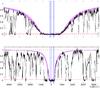 |
Fig. A.1
Voigt profile fits to the DLA: Lyman-α transition on top, Lyman-β at lower panel. The fit to the data with its uncertainty is shown in the shaded area. Vertical dashed lines mark the position of the H i components used for the fit, determined both from the wings of Lyman-α and Lyman-β and the profile of higher Lyman transitions. The observational error is shown at the bottom for reference. |
| Open with DEXTER | |
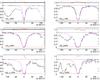 |
Fig. A.2
Voigt profile fits to H2J = 0. The fit to the data is represented by a line. Residuals of the fit are shown on top. The observational error is shown at the bottom for reference. Presence of residual flux is obvious in a few cases. |
| Open with DEXTER | |
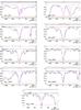 |
Fig. A.3
Voigt profile fits to H2J = 1. The fit to the data is represented by a line. Residuals of the fit are shown on top. The observational error is shown at the bottom for reference. |
| Open with DEXTER | |
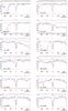 |
Fig. A.4
Voigt profile fits to H2J = 2. The fit to the data is represented by a line. Residuals of the fit are shown on top. The observational error is shown at the bottom for reference. |
| Open with DEXTER | |
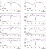 |
Fig. A.5
Voigt profile fits to H2J = 3. The fit to the data is represented by a line. Residuals of the fit are shown on top. The observational error is shown at the bottom for reference. |
| Open with DEXTER | |
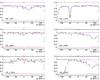 |
Fig. A.6
Voigt profile fits to H2J = 4 and 5. The fit to the data is represented by a line. Residuals of the fit are shown on top. The observational error is shown at the bottom for reference. |
| Open with DEXTER | |
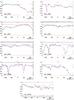 |
Fig. A.7
Selection of HD J = 0 absorption features. A tentative fit to the data is represented by a line for reference. Residuals of the fit are shown on top. The observational error is shown at the bottom for reference. |
| Open with DEXTER | |
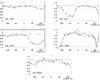 |
Fig. A.8
Selection of HD J = 1 absorption features. A tentative fit to the data is represented by a line for reference. Residuals of the fit are shown on top. The observational error is shown at the bottom for reference. |
| Open with DEXTER | |
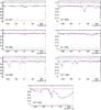 |
Fig. A.9
Voigt profile fits to carbon features. The fit to the data is represented by a line. Residuals of the fit are shown on top. The observational error is shown at the bottom for reference. |
| Open with DEXTER | |
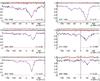 |
Fig. A.10
Multiple-component Voigt profile fits to high ionisation element profiles. The fit to the data is represented by a line. Residuals of the fit are shown in red on top when corresponding to the intervals used for the fit, and otherwise in black. The observational error is shown at the bottom for reference. |
| Open with DEXTER | |
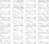 |
Fig. A.11
Multiple-component Voigt profile fits to low ionisation element profiles. The fit to the data is represented by a line. Residuals of the fit are shown on top, in red when corresponding to the intervals used for the fit, in black otherwise. The observational error is shown at the bottom for reference. C ii and O i are impossible to decompose because all features are heavily saturated. |
| Open with DEXTER | |
Appendix B: Transitions used for Δμ/μ and their redshifts
We summarise in Table B.1 the H2 lines used for the determination of Δμ/μ. We present the rest frame wavelength and sensitivity coefficients we used, the redshifts we have measured with a two-component model and Δμ/μ included as a free parameter of the fit, as well as the velocity shift with respect to the H2-bearing cloud redshift.
Laboratory wavelength of the set of H2 transitions that are fitted along with the best redshift and errors from Vogit profile analysis. The uncontaminated (CLEAN) H2 lines are highlighted in bold letters.
© ESO, 2014
Current usage metrics show cumulative count of Article Views (full-text article views including HTML views, PDF and ePub downloads, according to the available data) and Abstracts Views on Vision4Press platform.
Data correspond to usage on the plateform after 2015. The current usage metrics is available 48-96 hours after online publication and is updated daily on week days.
Initial download of the metrics may take a while.