| Issue |
A&A
Volume 562, February 2014
|
|
|---|---|---|
| Article Number | A45 | |
| Number of page(s) | 22 | |
| Section | Interstellar and circumstellar matter | |
| DOI | https://doi.org/10.1051/0004-6361/201321954 | |
| Published online | 04 February 2014 | |
Far-infrared molecular lines from low- to high-mass star forming regions observed with Herschel⋆
1 Max-Planck Institut für Extraterrestrische Physik (MPE), Giessenbachstr. 1, 85748 Garching, Germany
e-mail: This email address is being protected from spambots. You need JavaScript enabled to view it.
2 Leiden Observatory, Leiden University, PO Box 9513, 2300 RA Leiden, The Netherlands
3 Université de Bordeaux, Observatoire Aquitain des Sciences de l’Univers, 2 rue de l’Observatoire, BP 89, 33271 Floirac Cedex, France
4 CNRS, LAB, UMR 5804, 33271 Floirac Cedex, France
5 Centro de Astrobiología. Departamento de Astrofísica. CSIC-INTA. Carretera de Ajalvir, Km 4, 28850 Torrejón de Ardoz., Madrid, Spain
6 Kavli Institut for Astronomy and Astrophysics, Yi He Yuan Lu 5, HaiDian Qu, Peking University, 100871 Beijing, PR China
7 SRON Netherlands Institute for Space Research, PO Box 800, 9700 AV Groningen, The Netherlands
8 Kapteyn Astronomical Institute, University of Groningen, PO Box 800, 9700 AV Groningen, The Netherlands
9 Max-Planck-Institut für Radioastronomie, Auf dem Hügel 69, 53121 Bonn, Germany
Received: 24 May 2013
Accepted: 25 November 2013
Abstract
Aims. Our aim is to study the response of the gas-to-energetic processes associated with high-mass star formation and compare it with previously published studies on low- and intermediate-mass young stellar objects (YSOs) using the same methods. The quantified far-IR line emission and absorption of CO, H2O, OH, and [O i] reveals the excitation and the relative contribution of different atomic and molecular species to the gas cooling budget.
Methods. Herschel/PACS spectra covering 55–190 μm are analyzed for ten high-mass star forming regions of luminosities Lbol ~ 104−106 L⊙ and various evolutionary stages on spatial scales of ~104 AU. Radiative transfer models are used to determine the contribution of the quiescent envelope to the far-IR CO emission.
Results. The close environments of high-mass protostars show strong far-IR emission from molecules, atoms, and ions. Water is detected in all 10 objects even up to high excitation lines, often in absorption at the shorter wavelengths and in emission at the longer wavelengths. CO transitions from J = 14 − 13 up to typically 29 − 28 (Eu/kB ~ 580−2400 K) show a single temperature component with a rotational temperature of Trot ~ 300 K. Typical H2O excitation temperatures are Trot ~250 K, while OH has Trot ~ 80 K. Far-IR line cooling is dominated by CO (~75%) and, to a smaller extent, by [O i] (~20%), which becomes more important for the most evolved sources. H2O is less important as a coolant for high-mass sources because many lines are in absorption.
Conclusions. Emission from the quiescent envelope is responsible for ~45–85% of the total CO luminosity in high-mass sources compared with only ~10% for low-mass YSOs. The highest− J lines (Jup ≥ 20) originate most likely in shocks, based on the strong correlation of CO and H2O with physical parameters (Lbol, Menv) of the sources from low- to high-mass YSOs. The excitation of warm CO described by Trot ~ 300 K is very similar for all mass regimes, whereas H2O temperatures are ~100 K high for high-mass sources compared with low-mass YSOs. The total far-IR cooling in lines correlates strongly with bolometric luminosity, consistent with previous studies restricted to low-mass YSOs. Molecular cooling (CO, H2O, and OH) is ~4 times greater than cooling by oxygen atoms for all mass regimes. The total far-IR line luminosity is about 10-3 and 10-5 times lower than the dust luminosity for the low- and high-mass star forming regions, respectively.
Key words: infrared: ISM / ISM: jets and outflows / stars: protostars / molecular processes / astrochemistry
Appendices are available in electronic form at http://www.aanda.org
© ESO, 2014
1. Introduction
High-mass stars (M > 8 M⊙) play a central role in the energy budget, the shaping, and the evolution of galaxies (see review by Zinnecker & Yorke 2007). They are the main source of UV radiation in galaxy disks. Massive outflows and H ii regions are powered by massive stars and are responsible for generating turbulence and heating the interstellar medium (ISM). At the end of their lives, they inject heavy elements into the ISM that form the next generation of molecules and dust grains. These atoms and molecules are the main cooling channels of the ISM. The models of high-mass star formation are still strongly debated: these two competing scenarios are turbulent core accretion and “competitive accretion” (e.g. Cesaroni 2005). Molecular line observations are crucial to determining the impact of UV radiation, outflows, infall, and turbulence on the formation and evolution of the high-mass protostars and ultimately distinguish between those models.
Based on observations, the “embedded phase” of high-mass star formation may empirically be divided into several stages (e.g. Helmich & van Dishoeck 1997; van der Tak et al. 2000; Beuther et al. 2007): (i) massive prestellar cores (PSC); (ii) high-mass protostellar objects (HMPOs); (iii) hot molecular cores (HMC); and (iv) ultra-compact H ii regions (UCH ii). The prestellar core stage represents initial conditions of high-mass star formation, with no signatures of outflow/infall or maser activity. During the high-mass protostellar objects stage, infall of a massive envelope onto the central star and strong outflows indicate the presence of an active protostar. In the hot molecular core stage, large amounts of warm and dense gas and dust are seen. The temperature of T > 100 K in subregions <0.1 pc in size is high enough to evaporate molecules off the grains. In the final, ultra-compact H ii regions stage, a considerable amount of ionized gas is detected surrounding the central protostar.
The above scenario is still debated (Beuther et al. 2007), in particular whether stages (ii) and (iii) are indeed intrinsically different. The equivalent sequence for the low-mass young stellar objects (YSO) is better established (Shu et al. 1987; André et al. 1993, 2000). The embedded phase of low-mass protostars consists of (i) the prestellar core; (ii) Class 0, and (iii) Class I phases. The Class 0 YSOs are surrounded by a massive envelope and drive collimated jets/ outflows. In the more evolved Class I objects, the envelope is mostly dispersed and more transparent for UV radiation. The outflows are less powerful and have larger opening angles.
Low-mass sources can be probed at high spatial resolution due to a factor of 10 shorter distances, which allow us to study well-isolated sources and avoid much of the confusion due to clouds along the line of sight. The line emission is less affected by foreground extinction and therefore provides a good tool for studying the gas’s physical conditions and chemistry in the region. The slower evolutionary timescale results in a large number of low-mass YSOs compared to their high-mass counterparts, which is also consistent with observed stellar/core mass functions.
While low-mass YSOs are extensively studied in the far-infrared, first with the Infrared Space Observatory (ISO, Kessler et al. 1996) and now with Herschel (Pilbratt et al. 2010)1, the same is not the case for high-mass sources (see e.g. Helmich & van Dishoeck 1997; Vastel et al. 2001; Boonman & van Dishoeck 2003). For those, the best-studied case is the relatively nearby Orion BN-KL region observed with ISO’s Long- and Short-Wavelength Spectrometers (Clegg et al. 1996; de Graauw et al. 1996). Spectroscopy at long wavelengths (45–197 μm) shows numerous and often highly excited H2O lines in emission (Harwit et al. 1998), high-J CO lines (e.g., up to J = 43–42 in OMC-1 core, Sempere et al. 2000), and several OH doublets (Goicoechea et al. 2006), while the shorter wavelength surveys reveal the CO and H2O vibration-rotation bands and H2 pure rotational lines (van Dishoeck et al. 1998; Rosenthal et al. 2000). Fabry-Perot (FP) spectroscopy (λ/Δλ ~ 10 000, 30 km s-1) data show resolved P-Cygni profiles for selected H2O transitions at λ < 100 μm, with velocities extending up to 100 km s-1 (Wright et al. 2000; Cernicharo et al. 2006). At the shortest wavelengths (<45 μm) all pure rotational H2O lines show absorption (Wright et al. 2000). ISO spectra towards other high-mass star forming regions are dominated by atomic and ionic lines (see review by van Dishoeck 2004), similar to far-IR spectra of extragalactic sources (Fischer et al. 1999; Sturm et al. 2002).
The increased sensitivity and spectral and spatial resolution of the Photodetector Array Camera and Spectrometer (PACS; Poglitsch et al. 2010) onboard Herschel now allow detailed study of the molecular content of a larger sample of high-mass star forming regions. In particular, the more than an order of magnitude improvement in the spectral resolution over the ISO-LWS grating observing mode allows routine detections of weak lines against the very strong continuum of high-mass sources with Herschel, with line-to-continuum ratios below 1%.
The diagnostic capabilities of far-IR lines have been demonstrated by the recent results on low- and intermediate-mass YSOs and their outflows (Fich et al. 2010; Herczeg et al. 2012; Goicoechea et al. 2012; Manoj et al. 2013; Wampfler et al. 2013; Karska et al. 2013; Green et al. 2013). The CO ladder from J = 14–13 up to 49–48 and a few tens of H2O lines with a range of excitation energies are detected towards the Class 0 sources, NGC 1333 IRAS4B and Serpens SMM1 (Herczeg et al. 2012; Goicoechea et al. 2012). The highly-excited H2O 818–707 line at 63.3 μm (Eu/kB = 1071 K) is seen towards almost half of the Class 0 and I sources in the Karska et al. (2013) sample, even for bolometric luminosities as low as ~1 L⊙. Non-dissociative shocks and, to a lesser extent, UV-heating are suggested as the dominant physical processes responsible for the observed line emission (van Kempen et al. 2010; Visser et al. 2012; Karska et al. 2013). The contribution from the bulk of the quiescent warm protostellar envelope to the PACS lines is negligible for low-mass sources. Even for the intermediate-mass source NGC 7129 FIRS2, where the envelope contribution is higher, the other processes dominate (Fich et al. 2010).
In this paper, we present Herschel/PACS spectroscopy of ten sources that cover numerous lines of CO, H2O, OH, and [O i] lines obtained as part of the “Water in star forming regions with Herschel” (WISH) key program (van Dishoeck et al. 2011). WISH observed in total about 80 protostars at different evolutionary stages (from prestellar cores to circumstellar disks) and masses (low-, intermediate-, and high-mass) with both the Heterodyne Instrument for the Far-Infrared (HIFI; de Graauw et al. 2010) and PACS (Poglitsch et al. 2010). This paper focuses only on PACS observations of high-mass YSOs. It complements the work by van der Tak et al. (2013), which describes our source sample and uses HIFI to study spectrally resolved ground-state H2O lines towards all our objects. That paper also provides updated physical models of their envelopes.
The results for high-mass YSOs will be compared with those for low- and intermediate-mass young stellar objects, analyzed in a similar manner (Karska et al. 2013; Wampfler et al. 2013; Fich et al. 2010) in order to answer the following questions: How does far-IR line emission/absorption differ for high-mass protostars at different evolutionary stages? What are the dominant gas cooling channels for those sources? What physical components do we trace and what gas conditions cause the excitation of the observed lines? Are there any similarities with the low- and intermediate-mass protostars?
The paper is organized as follows. Section 2 introduces the source sample and explains the observations and reduction methods, Sect. 3 presents results that are derived directly from the observations, Sect. 4 focuses on the analysis of the data, Sect. 5 discusses our results in the context of the available models, and Sect. 6 summarizes the conclusions.
2. Observations and data reduction
We present spectroscopy observations of ten high-mass star forming regions collected with the PACS instrument on board Herschel in the framework of the WISH program. The sources have an average distance of ⟨ D ⟩ = 2.7 kpc and represent various stages of evolution, from the classical high-mass protostellar objects (HMPOs) to hot molecular cores (HMCs) and ultra-compact H ii regions (UC H ii). The list of sources and their basic properties are given in Table 1. Objects are shown in the sequence of increasing value of an evolutionary tracer,  , introduced in Bontemps et al. (1996). The sequence does not always correspond well with the evolutionary stages most commonly assigned to the sources in the literature (last column of Table 2), perhaps because multiple objects in different evolutionary stages are probed within our spatial resolution element (see e.g. Wyrowski et al. 2006; Leurini et al. 2013, for the case of G327-0.6).
Catalog information and source properties.
Far-IR line cooling by molecules and atoms in units of L⊙.
PACS is an integral field unit with a 5 × 5 array of spatial pixels (hereafter spaxels). Each spaxel covers  × , providing a total field of view of ~47′′ × 47′′. The focus of this work is on the central spaxel. The central spaxel probes similar physical scales as the full 5 × 5 array in the ten times closer low-mass sources. Full 5 × 5 maps for the high-mass sources, both in lines and continuum, will be discussed in future papers.
The range spectroscopy mode on PACS uses large grating steps to quickly scan the full 50–210 μm wavelength range with Nyquist sampling of the spectral elements. The wavelength coverage consists of three grating orders (1st: 102–210 μm; 2nd: 71–105 μm; or 3rd: 51–73 μm), two of which are always observed simultanously (one in the blue, λ < 105 μm, and one in the red, λ > 102 μm, parts of the spectrum). The spectral resolving power is R = λ/Δλ ≈ 1000–1500 for the first order, 1500–2500 for the second order, and 2500–5500 for the third order (corresponding to velocity resolution from ~75 to 300 km s-1).
Two nod positions were used for chopping 3′ on each side of the source. The comparison of the two positions was made to assess the influence of the off-source flux of observed species from the off-source positions, in particular for atoms and ions. The [C ii] fluxes are strongly affected by the off-position flux and saturated for most sources – we therefore limit our analysis of this species to the two sources with comparable results for both nods, AFGL2591 and NGC 7538-IRS1 (see Table 2).
Typical pointing accuracy is better than 2′′. However, two sources (G327-0.6 and W33A) were mispointed by a larger amount as indicated by the location of the peak continuum emission on maps at different wavelengths (for the observing log see Table A.1 in the Appendix). To account for the non-centric flux distribution on the integral field unit due to mispointing and to improve the continuum smoothness, for these sources two spaxels with maximum continuum levels are used (spaxel 11 and 21 for G327 and 23 and 33 for W33A). Summing a larger number of spaxels was not possible owing to a shift of line profiles from absorption to emission. The spatial extent of line emission/absorption will be analyzed in future papers.
We performed the basic data reduction with the Herschel Interactive Processing Environment v.10 (HIPE, Ott 2010). The flux was normalized to the telescopic background and calibrated using Neptune observations. Spectral flatfielding within HIPE was used to increase the S/N (for details, see Herczeg et al. 2012; Green et al. 2013). The overall flux calibration is accurate to ~20%, based on the flux repeatability for multiple observations of the same target in different programs, cross-calibrations with HIFI and ISO, and continuum photometry.
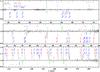 |
Fig. 1 Herschel/PACS continuum-normalized spectrum of W3 IRS5 at the central position. Lines of CO are shown in red, H2O in blue, OH in light blue, CH in orange, and atoms and ions in green. Horizontal magenta lines show spectral regions zoomed in Fig. C.1. |
Custom IDL routines were used to process the datacubes further. The line fluxes were extracted from the central spaxel (except G327-0.6 and W33A, see above) using Gaussian fits with fixed line width (for details, see Herczeg et al. 2012). Next, they were corrected for the wavelength-dependent loss of radiation for a point source (see PACS Observer’s Manual2). That approach is not optimal for the cases where emission is extended beyond the central spaxel, but that is mostly the case for atomic lines, which will be presented in a companion paper by Kwon et al. (in prep., hereafter Paper II). The uncertainty introduced by using the point-source correction factors for extended sources depends on the amount of emission in the surrounding ring of spaxels. The continuum fluxes are calculated using all 25 spaxels, except G327-0.6 where one spaxel was excluded due to saturation. In most cases, the tabulated values are at wavelengths near bright lines. They are calculated using spectral regions on both sides of the lines (but masking any features) and interpolated linearly to the wavelength of the lines. The fluxes are presented in Table B.1 in the Appendix. Our continuum fluxes are included in the spectral energy distribution fits presented in van der Tak et al. (2013), who used them to derive physical models for all our sources. Those models and associated envelope masses are used in this work in Sects. 5.1 and 5.3.
3. Results
Figure 1 shows the full normalized PACS spectrum with line identifications for W3 IRS5, a high-mass protostellar object with the richest molecular emission among our sources. Carbon monoxide (CO) transitions from J = 14–13 to J = 30–29 are detected, all in emission (see blow-ups of high-J CO lines in Figs. C.1 and C.2). Water-vapor (H2O) transitions up to Eup ~ 1000 K are detected (e.g. 716 − 625 at 66.1 μm, see blow-ups in Fig. C.1). At wavelengths shortwards of ~90 μm, many H2O lines are seen in absorption, but those at longer wavelengths are primarily in emission.
Seven hydroxyl (OH) doublets up to Eup ≈ 618 K are seen3. All lines within the  ladder (119, 84, and 65 μm doublets; see Fig. 1 in Wampfler et al. 2013) are strong absorption lines. The
  ladder lines (163 and 71 μm) are seen in emission. The cross-ladder transitions at 79 μm (OH 1/2,1/2–3/2,3/2, Eup ≈ 180 K) and 96 μm (OH 3/2,1/2–5/2,3/2, Eup ≈ 270 K) are absorption and emission lines, respectively. Only the ground-rotational lines of methylidyne (CH) are detected at 149 μm in absorption. The [O i] transitions at 63 μm and 145 μm are both strong emission lines in W3 IRS5. That is not always the case for other sources in our sample. The [O i] line at 63 μm, where the velocity resolution of PACS is at its highest (~90 km s-1), shows a variety of profiles (see Fig. 2): pure absorption (G327-0.6, W51Ne1, G34.26, W33A), regular P-Cygni profiles (AFGL2591, NGC 6334-I), hints of inverse P-Cygni profiles in DR21(OH) and pure emission (W3 IRS5, NGC 7538-I1, G5.89). The [O i] line at 145 μm, however, is always detected in emission. The P-Cygni profiles resolved on velocity scales of ~100 km s-1 resemble the high-velocity line wings observed in ro-vibrational transitions of CO in some of the same sources (Mitchell et al. 1990; Herczeg et al. 2011), suggested to originate in the wind impacting the outflow cavities. Not all absorption needs to be associated with the source, however: it can also be due to foreground absorption (e.g. outflow lobe or the ISM). For example, ISO Fabry Perot and new Herschel/HIFI observations of H2O and OH in Orion also show line wings in absorption/emission extending to velocities up to ~100 km s-1 (Cernicharo et al. 2006; Goicoechea et al. 2006, Choi et al. in prep.), but the ISO-LWS Fabry-Perot observations of Orion did not reveal any P-Cygni profiles in the [O i] 63 μm line.
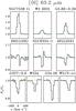 |
Fig. 2 Herschel/PACS profiles of the [O i] 63.2 μm line at central position. |
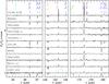 |
Fig. 3 Normalized spectral regions of all our sources at the central position at 64–68, 148–157, and 169–182 μm. Objects are shown in the evolutionary sequence, with the most evolved ones on top. Lines of CO are shown in red, H2O in blue, OH in light blue, CH in orange, and NH3 and C3 in green. Spectra are shifted vertically to improve the clarity of the figure. |
A comparison of selected line-rich parts of the spectra for all our sources is presented in Fig. 3. The spectra are normalized by the continuum emission to better visualize the line absorption depths. However, the unresolved profiles of PACS underestimate the true absorption depths and cannot be used to estimate the optical depths. The 64–68 μm segment covers the highly-excited H2O lines at 66.4, 67.1, and 67.3 μm (Eup ≈ 410 K); high-J CO lines at 65.7 (J = 40–39) and 67.3 (J = 39–38); and the OH J = 9/2 − 7/2 (Eup ≈ 510 K) doublet at 65 μm. The low-lying H2O lines are detected for all sources. The high-J CO lines are not detected in this spectral region. The OH doublet is detected for six out of ten sources (see also Fig. C.3 in the Appendix).
The main lines seen in the 148–157 μm region are CH  J = 3/2–
 J = 1/2 transition at 149 μm (in absorption), CO 17–16, and H2O 322 − 313 line at 156.2 μm (Eup ≈ 300 K). Weak absorption lines at ~155–156 μm seen towards the hot core G327-0.6 are most likely C3 ro-vibrational transitions (Cernicharo et al. 2000, Paper II).
The most commonly detected lines in the 170–182 μm spectral region include the CO 15–14 line and the H2O lines at 174.6, 179.5, and 180.5 μm (Eup ≈ 100–200 K). The profiles of H2O lines change from object to object: the H2O 212 − 101 line at 179.5 μm is in absorption for all sources except W3 IRS5; the H2O 221 − 112 at 180.5 μm is in emission for the three most evolved sources (top 3 spectra in Fig. 3). The ammonia line at ~170 μm, NH3 (3,2)a-(2,2)s, is detected toward four sources (G327-0.6, W51N-e1, G34.26, and NGC 6334-I). An absorption line at ~181 μm corresponds to H O 212 − 101 and/or H3O+
 lines (Goicoechea & Cernicharo 2001). Extended discussion of ions and molecules other than CO, H2O, and OH will appear in Paper II.
Line profiles of H2O observed with HIFI show a variety of emission and absorption components that are not resolved by PACS (Chavarría et al. 2010; Kristensen et al. 2012; van der Tak et al. 2013). The only H2O lines observed in common by the two instruments within the WISH program are the ground-state transitions: 212 − 101 at 179.5 μm (1670 GHz) and 221 − 112 at 180.5 μm (1661 GHz), both dominated by absorptions and therefore not optimal for estimating to what extent a complex water profile is diluted at the PACS spectral resolution. However, HIFI observations of the lines between excited rotational states, which dominate our detected PACS lines, are generally in emission at the longer wavelengths probed by HIFI. In the case of 12CO 10–9, the line profiles of YSOs observed with HIFI consist of a broad outflow and a narrow quiescent component with the relative fraction of the integrated intensity of the narrow to broad components being typically 30–70% for low-mass sources (Yıldız et al. 2013). For the single case of a high-mass YSO, W3 IRS5, this fraction is about 50% (San José-García et al. 2013).
To summarize, PACS spectra of high-mass sources from our sample show detections of many molecular lines up to high excitation energies. CO, H2O, OH, and CH lines are seen toward all objects, whereas weaker lines of other molecules are detected toward fewer than half of the sources. CO lines are always seen in emission, CH in absorption, and other species show different profiles depending on the transition and the object. Table C.1 shows the CO line fluxes for all lines in the PACS range.
4. Analysis
4.1. Far-IR line cooling
Emission lines observed in the PACS wavelength range are used to calculate the contribution of different species to the total line cooling from high-mass protostars. Our goal is to compare the cooling of warm gas by molecules and atoms with the cooling by dust and connect them with the evolutionary stages of the objects. Relative contributions to the cooling between different molecules are also determined, which can be an indicator of the physical processes in the environments of young protostars (e.g. Nisini et al. 2002; Karska et al. 2013).
We define the total far-IR line cooling (LFIRL) as the sum of all emission line luminosities from the fine-structure [O i] lines (at 63 and 145 μm) and the detected molecules, following Nisini et al. (2002) and Karska et al. (2013). [C ii], the most important line coolant of diffuse interstellar gas, is also expected to be a significant cooling agent in high-mass star forming regions and extragalactic sources. It is not explicitly included in our analysis, however, because the calculated fluxes are strongly affected by off-source emission and often saturated (see also Sect. 2). The emitted [C ii] luminosity is shown below for only two sources, where reliable fluxes were obtained. Cooling in other ionic lines such as [O iii], [N ii], and [N iii] is also excluded, due to the off-position contamination and the fact that those lines trace a different physical component than the molecules and [O i]. Since the only molecules with emission lines are CO, H2O, and OH, the equation for the total far-IR line cooling can be written as LFIRL = LOI + LCO + LH2O + LOH.
Table 2 summarizes our measurements. The amount of cooling by dust is described by the bolometric luminosity and equals ~104 − 105 L⊙ for our sources (van der Tak et al. 2013). The total far-IR line cooling ranges from ~1 to ~40 L⊙, several orders of magnitude less than the dust cooling. Relative contributions of oxygen atoms and molecules to the gas cooling are illustrated in Fig. 4. Atomic cooling is largest for the more evolved sources in our sample (see Table 1), in particular for NGC 7538 IRS1 and AFGL2591, where it is the dominant line-cooling channel. For those two sources, additional cooling by [C ii] is determined and amounts to ~10–25% of LFIRL (Table 2). Typically, atomic cooling accounts for ~20% of the total line far-IR line cooling. Molecular line cooling is dominated by CO, which is responsible for ~15 up to 85% of LFIRL, with a median contribution of 74%. H2O and OH median contributions to the far-IR cooling are less than 1%, because many of their transitions are detected in absorption. Assuming that the absorptions arise in the same gas, as found for the case of Orion (Cernicharo et al. 2006), they therefore do not contribute to the cooling, but to heating the gas. Still, the contribution of H2O to the total far-IR cooling increases slightly for more evolved sources, from ~5% (DR21(OH)) to 30% (W3IRS5), whereas no such trend is seen for OH.
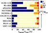 |
Fig. 4 Relative contributions of [O i] (dark blue), CO (yellow), H2O (orange), and OH (red) cooling to the total far-IR gas cooling at central position are shown from left to right horizontally for each source. The objects follow the evolutionary sequence with the most evolved sources on top. |
CO, H2O, and OH rotational excitation.
4.2. Molecular excitation
Detections of multiple rotational transitions of CO, H2O, and OH allow us to determine the rotational temperatures of the emitting or absorbing gas using Boltzmann diagrams (e.g. Goldsmith & Langer 1999). For H2O and OH, the densities are probably not high enough to approach a Boltzmann distribution and therefore the diagrams presented below are less meaningful.
Emission line fluxes are used to calculate the number of emitting molecules,  , for each molecular transition using Eq. (1), assuming that the lines are optically thin. Here, Fλ denotes the flux of the line at wavelength λ, d is the distance to the source, A the Einstein coefficient, c the speed of light, and h Planck’s constant:
  (1)The base-10 logarithm of over degeneracy of the upper level gu is shown as a function of the upper level energy, Eu, in Boltzmann diagrams (Figs. 5 and 6). The rotational temperature is calculated in a standard way, from the slope b of the linear fit to the data in the natural logarithm units, Trot = −1/b.
Because the size of the emitting region is not resolved by our instrument, the calculation of column densities requires additional assumptions and therefore only the total numbers of emitting molecules is determined. The formula for the total number of emitting molecules,  , is derived from the expression for total column density, Ntot = Q·exp(a), where Q is the partition function for the temperature and a the y-intercept. Correcting for a viewing angle, Ω = d2/πR2, and multiplying by the gas emitting area of radius R, yields
  (2)For details, see e.g. Karska et al. (2013) and Green et al. (2013).
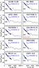 |
Fig. 5 Rotational diagrams of CO for all objects in our sample. The base-10 logarithm of the number of emitting molecules from a level u, |
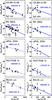 |
Fig. 6 Rotational diagrams of H2O calculated using emission lines (left column) and absorption lines (right column), respectively. For emission line diagrams, the logarithm with base 10 of total number of molecules in a level u, |
For absorption lines, column densities, Nl, are calculated from line equivalent widths, Wλ, using Eq. (3) (e.g. Wright et al. 2000).  (3)This relation assumes that the lines are optically thin, the covering factor is unity, and the excitation temperature Tex ≪ hc/kλ for all lines. Some of the emission/absorption lines are likely P-Cygni profiles (Cernicharo et al. 2006) that are not resolved with PACS and which we assume to be pure emission/absorbing lines.
The natural logarithm of Nl over the degeneracy of the lower level, gl, is shown in the Boltzmann diagrams as a function of the lower level energy, El (Figs. 6, 7, and 9). Rotational temperatures and total column densities are calculated in the same way as for the emission lines (see above).
In the following sections, the excitation of CO, H2O, and OH are discussed separately. Table 3 summarizes the values of rotational temperatures, Trot, and total numbers of emitting molecules or column densities, for those species.
4.2.1. CO
Figure 5 shows CO rotational diagrams for all our sources. CO detections, up to J =30-29 (Eu = 2565 K), are described well by single rotational temperatures in the range from 220 K (AFGL2591 and NGC 7538 IRS1) to ~370 K (W3IRS5 and G34.26+0.15) and the average of Trot,CO ~ 300(23) ± 60 K4. The highest temperatures are seen for objects where high-J CO transitions with Eu > 2000 K are detected.
Temperatures of ~300 K are attributed to the “warm” component in low-mass YSOs (e.g. Goicoechea et al. 2012; Karska et al. 2013; Green et al. 2013), where they are calculated using transitions from Jup = 14 (Eu = 580 K) to 24 (Eu = 1660 K). In those sources, a break around Eu ~ 1800 K in the rotational diagram is noticeble (see vertical line in Fig. 5) and Jup ≥ 25 transitions are attributed to the “hot” component. Such a turning point is not seen in the diagrams of our high-mass sources with detections extending beyond the J = 24−23 transition.
In NGC 7538 IRS1, a possible break is seen around Eu ~ 1000 K. A two-component fit to the data results in rotational temperatures Trot1 ~ 160 ± 10 K and Trot2 ~ 370 ± 35 K. The latter temperature is consistent within errors with the “warm” component seen towards low-mass sources. The colder temperature resembles the ~70−100 K “cool” component seen in Jup ≤ 14 transitions (e.g. Goicoechea et al. 2012; Karska et al. 2013; van der Wiel et al. 2013), detected at longer wavelengths than the PACS range.
The absence of the hot component toward all our sources is not significant according to the calculated upper limits. In addition to limited S/N and line-to-continuum ratio, there are other effects that may prevent the hot component from being detected. These include the fact that the continuum becomes more optically thick at the shorter wavelengths (see also below) and/or a smaller filling factor of the hot component in the PACS beam compared with low-mass sources. More generally, both the “warm” and “hot” components could still be part of a single physical structure as proposed in Neufeld (2012).
The average logarithm of the number of emitting (warm) CO molecules,  , is similar for all objects, and equals 52.4(0.1) ± 0.5. Values of in the range from 51.6 to 53.1 are derived. DR21(OH), one of the lowest bolometric luminosity sources in our sample, exhibits one of the lowest
  (CO) contents, whereas the highest CO content is found for W51N-e1, the most luminous source.
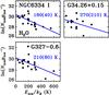 |
Fig. 7 Rotational diagrams of H2O calculated using absorption lines. A single-component fit is used to calculate the temperature shown in the panels. |
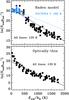 |
Fig. 8 Top: rotational diagram of H2O calculated assuming a kinetic temperature T = 1000 K, H2 density n = 106 cm-3, H2O column density 2 × 1016 cm-2, and line width ΔV = 5 km s-1. Lines observed in absorption in NGC 6334-I are shown in blue. Fits are done to all lines in the PACS range included in the LAMDA database (Schöier et al. 2005) (in black) and to the NGC 6334-I lines (in blue). Darker shades denote optically thin lines. Bottom: the same as above, but assuming an H2O column density 1012 cm-2, such that all lines are optically thin. |
4.2.2. H2O
Figure 6 shows rotational diagrams of H2O calculated for five sources with H2O lines detected both in emission and in absorption. Because the emitting region is not resolved by our observations, the diagrams calculated using the emission and absorption lines are shown separately. Figure 7 shows H2O diagrams for the three sources where all H2O lines are seen in absorption.
The rotational diagrams show substantial scatter, greater than the errors of individual data points, caused by large opacities, subthermal excitation (see Herczeg et al. 2012 and below), and possible radiation excitation by far-IR dust emission pumping. The determination of rotational temperatures is therefore subject to significant errors when only a limited number of lines is detected. In Table 3 H2O temperatures calculated using at least ten lines are indicated in boldface. Ro-vibrational spectra of H2O from ISO-SWS towards massive protostars (four of them in common with our sample) show rotational temperatures of H2O as high as 500 K, in agreement with the errors with our measurements (Boonman & van Dishoeck 2003).
The largest number of H2O lines is detected in the two most evolved sources – G5.89-0.39 and W3 IRS5. Single component fits to 12 and 37 water emission lines, respectively, give similar rotational temperatures of ~250 K (see Fig. 6), with no systematic differences between o-H2O and p-H2O lines. Rotational temperatures determined for the remaining sources, with at least five detections of H2O in emission, are higher, Trot ~ 300 − 450 K, but are less accurate.
Rotational temperatures calculated from a single component fit to the absorption line diagrams are ~200 K for all sources. They are in good agreement with the values obtained from the emission diagrams for G5.89-0.39 and W3 IRS5, suggesting that all H2O lines originate in the same physical component (see e.g. Cernicharo et al. 2006). In such a scenario, the column densities should also agree, and the comparison of the total number of molecules calculated from emission lines and columns determined from the absorption lines yields the size of the emitting region, R. The radius of the H2O emitting area under that condition equals ~3 arcsec for G5.89-0.39 and W3 IRS5 (see Table 3).
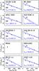 |
Fig. 9 Rotational diagrams of OH calculated using absorption lines, similar to Fig. 7 for H2O. The single component fit to all OH transitions detected in absorption is shown with a solid line with the corresponding temperature. A separate single component fit is done for the OH |
To assess the effects of optical depth and subthermal excitation on the derived temperatures from the absorption lines, equivalent widths of lines are calculated using the radiative transfer code Radex (van der Tak et al. 2007) and translated to column densities using Eq. (3). The adopted physical conditions of Tkin = 1000 K and n = 106 cm-3 are typical of warm, shocked region where water is excited (Goicoechea et al. 2012). The models were calculated using all H2O lines in the PACS range included in the LAMDA database (Schöier et al. 2005). The latest available H2O collisional coefficients are used (Daniel et al. 2011, and references therein).
Figure 8 shows the “theoretical” rotational diagrams calculated for low and high column densities. A single component fit to all lines in the high column density model gives a temperature of ~120 K, consistent with subthermal excitation, and a total column density of 1.2 × 1015 cm-2 (lnNlow ~ 34.7), an order of magnitude lower than the input column. A separate fit to the lines detected in NGC 6334-I gives a temperature of ~180 K and a slightly higher column density (1.9 × 1015 cm-2). These observed lines are typically highly optically thick with τ ~ few tens, up to 100.
In the low column density model all lines are optically thin. A fit to all lines gives a temperature of ~120 K, similar to the high column density model. The level populations are clearly subthermal (Trot ≪ Tkin), resulting in the scatter in the diagram. These examples illustrate the difficulty in using the inferred rotational temperatures to characterize a complex environment of high-mass star forming regions.
The continuum opacity at PACS wavelengths is typically of the order of a few in the observed sources, as indicated by the source structures derived by van der Tak et al. (2013), and becomes higher at shorter wavelengths. This implies that the absorbing H2O is on the frontside of the source. Also, any emission at short wavelengths must originate outside the region where the dust is optically thick.
4.2.3. OH
Figure 9 presents rotational diagrams of OH calculated using absorption lines. A single component is fitted to all detected lines. A separate fit is done for the lines originating in the ladder, which are mostly collisionally excited. This fit excludes the intra-ladder 79 μm doublet, connecting with the ground state, which readily gets optically thick (Wampfler et al. 2013). A possible line-of-sight contribution by unrelated foreground is expected in the ground-state 119 μm line, which is included in the fit. The resulting rotational temperatures for each source are shown in Table 3, separately for those two fits.
The average rotational temperature for the ladder is very similar for all objects and equals 100(12) ± 7 K. The inclusion of all OH doublets results in lower temperatures, Trot,OH ~ 79(22) ± 6 K.
5. Discussion: from low to high mass
5.1. Origin of CO emission
Several physical components have been proposed as a source of far-IR CO emission in isolated low-mass young stellar objects: (i) the inner parts of the quiescent envelope, passively heated by a central source (Ceccarelli et al. 1996; Doty & Neufeld 1997); (ii) gas in cavity walls heated by UV photons (van Kempen et al. 2009; van Kempen et al. 2010; Visser et al. 2012); (iii) currently shocked gas along the outflow walls produced by the protostellar wind-envelope interaction (van Kempen et al. 2010; Visser et al. 2012; Karska et al. 2013).
The quiescent envelope of high-mass protostars is warmer and denser than for low-mass YSOs, and therefore its contribution to the far-IR CO emission is expected to be greater. In this section, we determine this contribution for a subsample of our sources using the density and temperature structure of each envelope obtained by van der Tak et al. (2013).
In this work, the continuum emission for all our objects is modeled using a modified 3D Whitney-Robitaille continuum radiative transfer code (Robitaille 2011; Whitney et al. 2013). For simplicity, the van der Tak et al. models do not contain any cavity or disk, and assume a spherically symmetric power law density structure of the envelope, n ∝ r− p, where p is a free parameter. The size and mass of the envelope and the power law exponent, p, are calculated by best-fit comparison to the spectral energy distributions and radial emission profiles at 450 and 850 μm (Shirley et al. 2000). The models solve for the dust temperature as function of radius and assume that the gas temperature is equal to the dust temperature. For more detailed discussion, see van der Tak et al. (2013).
The envelope temperature and density structure from van der Tak et al. (2013) is used as input to the 1D radiative transfer code RATRAN (Hogerheijde & van der Tak 2000) in order to simultaneously reproduce the strengths of optically thin C18O lines from J = 2–1 to 9–8 (following the procedure in Yıldız et al. 2010, 2012). The free parameters include C18O constant abundance X0 and the line width, FWHM. For three sources, a “jump” abundance profile structure is needed, described by the evaporation temperature Tev and inner abundance Xin. The parameters derived from the fits are summarized in Table 4; the C18O observations are taken from San José-García et al. (2013), while the modeling details and results for all our objects will be presented in San José-García (in prep.).
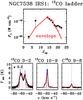 |
Fig. 10 Top: comparison of integrated line fluxes of 12CO observed by Herschel/PACS and from the ground (black dots with errorbars) and the predictions of the quiescent envelope passively heated by the luminosity of the source (red crosses) for NGC 7538-IRS1. Bottom: the same model compared with the JCMT 12CO 3–2 and Herschel/HIFI 13CO 10–9 and C18O 9–8 observed line profiles. An additional model including an outflow component is shown in blue dashed line. |
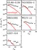 |
Fig. 11 Comparison of integrated line fluxes of CO observed by PACS only (black dots with error bars) and the predictions of the quiescent envelope passively heated by the luminosity of the source (red crosses). |
The parameters from Table 4 are used as input for the RATRAN models of 12CO. The integrated 12CO line emission obtained from RATRAN is convolved with the telescope beam and compared with observed line fluxes.
Figure 10 compares the envelope model for NGC 7538 IRS1 with the 12CO Jup = 14 to 22 observations from Herschel/PACS, CO 3–2 (in 14′′ beam, San José-García et al. 2013), and CO 7–6 (in 8′′ beam, Boonman et al. 2003) from the James Clerk Maxwell Telescope. By design, the model fits the line profile of C18O 9–8 (San José-García et al. 2013, from Herschel/HIFI) shown in the bottom of Fig. 10. The pure envelope model slightly underproduces the 13CO 10–9 line, because it does not include any broad entrained outflow component (Tex ~ 70 K, Yıldız et al. 2013). Adding such an outflow to the model (see Mottram et al. 2013) provides an excellent fit to the total line profile. For the case of 12CO, the pure envelope model reproduces the 3–2 and 7–6 lines within a factor of two, with the discrepancy again caused by the missing outflow in the model. This envelope model reproduces the CO-integrated intensities for transitions up to Jup = 18, but the larger J CO fluxes are underestimated by a large factor.
Comparison of the observed and modeled integrated 12CO line emission for the remaining sources from Table 4 is shown in Fig. 11. As found for the case of NGC 7538 IRS1, the contribution of the quiescent envelope emission can be as high as 70–100% of that of the J = 15–14 line but decreases sharply for the higher-J transitions. Only 3% to 22% of CO J = 22–21 line emission is reproduced by the envelope models. In total ~50% to 100% of observed total FIR CO luminosity can be explained by the envelope emission (see Table 5).
This contribution is much greater than for low-mass YSOs, where the quiescent envelope is responsible for only up to 7% of the total CO emission (Visser et al. 2012). Still, even for the high-mass sources, an additional physical component is needed to explain the excitation of the highest-J CO lines. The broad line profiles of high-J (J ≥ 10) CO lines (San José-García et al. 2013) argue in favor of a shock contribution to the far-IR emission in 12CO. There may also be a contribution from UV-heating of the outflow cavities by the photons from the protostellar accretion shocks or produced by high velocity shocks inside the cavities as found for low-mass YSOs (Visser et al. 2012), but this component is distinguished best by high-J13CO lines (van Kempen et al. 2009). Physical models similar to those developed for low-mass sources by Visser et al. (2012), which include the different physical components, are needed to compare the relative contribution of the envelope emission, shocks, and UV-heating in the high-mass sources, but this goes beyond the scope of this paper.
Far-IR CO emission: observations and envelope models.
5.2. Molecular excitation
The basic excitation analysis using Boltzmann diagrams in Sect. 4.2 shows remarkably similar rotational temperatures of each molecule for all our high-mass sources, irrespective of their luminosity or evolutionary stage. The average values of those temperatures are 300 K for CO, 220 K for H2O, and 80 K for OH.
Figure 12 presents our results in the context of low- and intermediate-mass YSOs studies by Fich et al. (2010), Herczeg et al. (2012), Goicoechea et al. (2012), Manoj et al. (2013), Wampfler et al. (2013), Karska et al. (2013), Green et al. (2013), and Lee et al. (2013). Rotational temperatures from the Water In Star forming regions with Herschel (WISH), the Dust, Ice, and Gas In Time (DIGIT), and the Herschel Orion Protostar Survey (HOPS) programs are shown separately. OH rotational temperatures of NGC 1333 I4B, Serpens SMM1, and L1448 are taken from the literature, whereas temperatures for the two additional low-mass YSOs and four intermediate-mass YSOs are calculated in Appendix B based on the line fluxes from Wampfler et al. (2013).
Rotational temperatures of CO are remarkably similar for most sources in the luminosity range from 10-1 to 106 L⊙ and equal to ~300–350 K. For the high-mass sources, this refers to the shocked component, not the quiescent envelope component discussed in Sect. 5.1. To explain such temperatures in low-mass YSOs, two limiting solutions for the physical conditions of the gas have been proposed: (i) CO is subthermally excited in hot (Tkin ≥ 103 K), low-density (n(H2) ≤ 105 cm-3) gas (Neufeld 2012; Manoj et al. 2013); or (ii) CO is close to LTE in warm (Tkin ~ Trot) and dense (n(H2) > ncrit ~ 106 cm-3) gas (Karska et al. 2013). The low-density scenario (i) in the case of even more massive protostars studied in this work is probably unlikely. Even though no 13CO lines are detected in our PACS spectra, three of our high-mass protostars were observed in the fundamental v = 1 − 0 vibration-rotation bands of CO and 13CO (Mitchell et al. 1990). The Boltzmann distribution of high-J populations of 13CO, indicated by a single component on rotational diagrams, implies densities above 106 cm-3 for W33A and NGC 7538-I1 and >107 cm-3 for W3 IRS5.
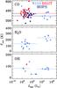 |
Fig. 12 Rotational temperatures of CO, H2O, and OH for low- to high-mass star forming regions. WISH, DIGIT, and HOPS team’s results with PACS are shown in blue, red, and navy blue, respectively. Dotted lines show the median values of the rotational temperature from each database; for the case of WISH, the median is calculated separately for objects with Lbol < 103 L⊙ and Lbol > 103 L⊙, except for OH where intermediate-mass YSOs covering 103 > Lbol > 50 L⊙ are also shown separately. The CO and H2O excitation of intermediate-mass sources has not yet been surveyed with Herschel. |
Rotational temperatures of H2O increase for the more massive and more luminous YSOs from about 120 K to 220 K (Fig. 12). The similarity between the temperatures obtained from the absorption and emission lines argues that they arise in the same physical component in high-mass YSOs (see also Cernicharo et al. 2006). Owing to the high critical density, the water lines are most likely subthermally excited in both low- and high-mass YSOs (see discussion in Sect. 4.2.2), but in the denser environment of high-mass protostars, the gas is closer to LTE and therefore the rotational temperatures are higher. High optical depths of H2O lines drive the rotational temperatures to higher values, both for the low- and high-mass YSOs. Lines are in emission, when the angular size of the emitting region (ΔΩL) multiplied by the blackbody at excitation temperature is larger than the continuum flux at the same wavelength, 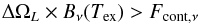 (4)and are in absorption in the opposite case.
Rotational temperatures of OH show a broad range of values for low-mass YSOs (from about 50 to 150 K), whereas they are remarkably constant for intermediate-mass YSOs (~35 K; see Appendix D) and high-mass YSOs (~80 K). The low temperatures found towards the intermediate-mass YSOs may be a result of the different lines detected towards those sources rather than a different excitation mechanism.
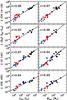 |
Fig. 13 Correlations of line emission with bolometric luminosity (left column) and envelope mass (right column) from top to bottom: CO 14–13, H2O 303–212, [O i] at 145 μm and OH 163 μm line luminosities. Low- and intermediate-mass young stellar objects emission is measured over 5 × 5 PACS maps. Red and blue circles show Class 0 and Class I low-mass YSOs from Karska et al. (2013). Blue diamonds show intermediate-mass YSOs from Wampfler et al. (2013; O and OH lines) and from Fich et al. (2010; CO and H2O line). High-mass YSOs fluxes are measured in the central position and shown in black. Pearson coefficient r is given for each correlation. |
5.3. Correlations
Figure 13 shows relations between selected line luminosities of CO, H2O, and [O i] transitions and the physical parameters of the young stellar objects. Our sample of objects is extended to the low-mass deeply embedded objects studied with PACS in Herczeg et al. (2012), Goicoechea et al. (2012), Wampfler et al. (2013), and Karska et al. (2013) and intermediate-mass objects from Fich et al. (2010) and Wampfler et al. (2013). This allows us to study a broad range of luminosities from ~1 to 106 L⊙, and envelope masses, from 0.1 to 104 M⊙.
The typical distance to low-mass sources is 200 pc and 3 kpc to high-mass sources. For this comparison, the full PACS array maps of low-mass regions are taken (~50′′), which corresponds to spatial scales of 104 AU, hence only a factor of 3 smaller than the central spaxel (~10′′) observation of high-mass objects. On the other hand, the physical sizes of the low-mass sources are smaller than those of high-mass sources by a factor that is comparable to the difference in average distance of low- and high-mass sources, so one could argue that one should compare just the central spaxels for both cases. Using only the central spaxel for the low-mass YSOs does not affect the results, however (see Fig. 9 in Karska et al. 2013).
The choice of CO, H2O, OH, and [O i] transitions is based on the number of detections of those lines in both samples and their emission profiles. The strengths of the correlations are quantified using the Pearson coefficient, r. For the number of sources studied here, the 3σ correlation corresponds to r ≈ 0.6 and 5σ correlation to r ≈ 0.95.
Figure 13 shows strong, 5σ correlations between the selected line luminosities and bolometric luminosities, as well as envelope masses. The more luminous the source, the higher is its luminosity in CO, H2O, and [O i] lines. Similarly, the more massive is the envelope surrounding the growing protostar, the larger is the observed line luminosity in those species. The strength of the correlations over such broad luminosity ranges and envelope masses suggests that the physical processes responsible for the line emission are similar.
In the case of low-mass young stellar objects, Karska et al. (2013) link the CO and H2O emission seen with PACS with the non-dissociative shocks along the outflow walls, most likely irradiated by the UV photons. The [O i] emission, on the other hand, was mainly attributed to the dissociative shocks at the point of direct impact of the wind on the dense envelope. In the high-mass sources, the envelope densities and the strength of radiation are higher, but all in all the origin of the emission can be similar.
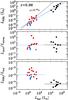 |
Fig. 14 From top to bottom: (1) total far-IR line cooling; (2) ratio of molecular to atomic cooling; (3) gas-to-dust cooling ratio, LFIRL/Lbol, where LFIRL = Lmol + Latom; as a function of bolometric luminosity. Low-mass YSOs are shown in red (Class 0) and blue (Class I), whereas high-mass ones are in black. |
5.4. Far-IR line cooling
Figure 14 compares the total far-IR cooling in lines, its molecular and atomic contributions, and the cooling by dust for the YSOs in the luminosity range from ~1 to 106 L⊙. The far-IR line cooling, LFIRL, correlates strongly (5σ) with the bolometric luminosity, Lbol, in agreement with studies on low-mass YSOs (Nisini et al. 2002; Karska et al. 2013). Under the assumption that LFIRL is proportional to the shock energy, the strong correlation between Lbol and LFIRL has been interpreted by Nisini et al. (2002) as a result of the jet power/velocity being correlated with the escape velocity from the protostellar surface or an initial increase in the accretion and ejection rate.
The ratio of molecular and atomic line cooling, Lmol/Latom, is similar for YSOs of different luminosities, although a large scatter is present. Cooling in molecules is about four times higher than cooling in oxygen atoms. If cooling by [C ii] was included in the atomic cooling, the Lmol/Latom ratio would decrease for the high-mass sources. In low-mass YSOs, the [C ii] emission accounts for less than 1% of the total cooling in lines (Goicoechea et al. 2012, for Ser SMM1). In the high-mass sources, this contribution is expected to be higher due to the carbon ionizing and CO dissociating FUV radiation. In Sect. 4.1 we estimate the [C ii] cooling in two high-mass sources to 10–25% of LFIRL.
The ratio of cooling by gas (molecular and atomic lines) and dust (Lbol) decreases from 1.3 × 10⁻³ to 6.2 × 10⁻⁵ from low to high-mass YSOs. It reflects that H2O and, to a smaller extent, OH contribute less to the line luminosity in the high-mass sources, because many of its lines are detected in absorption. The detection of H2O and OH lines in absorption proves that IR pumping is at least partly responsible for the excitation of these molecules and the resulting emission lines (e.g. Goicoechea et al. 2006; Wampfler et al. 2013). When collisions play a marginal role, even the detected emission lines of those species do not necessarily cool the gas.
The above numbers do not include cooling from molecules outside the PACS wavelength range. This contribution can be significant for CO, where for low-mass sources the low-J lines are found to increase the total CO line luminosity by about 30% (Karska et al. 2013). Thus, the CO contribution to the total gas cooling is likely to be even larger than suggested by Table 2.
6. Conclusions
We have characterized the central position Herschel/PACS spectra of ten high-mass protostars and compared them with the results for low- and intermediate-mass protostars analyzed in a similar manner. The conclusions are as follows:
-
1.
Far-IR gas cooling of high-mass YSOs is dominated by CO(from ~15 to 85% of total far-IR line cooling, with a median contribution of 74%) and to a smaller extent by [O i] (with median value ~20%). H2O and OH median contributions to the far-IR cooling are less than 1%. In contrast, for low-mass YSOs, the H2O, CO, and [O i] contributions are comparable. The effective cooling by H2O is reduced because many far-IR lines are in absorption. The [O i] cooling increases for more evolved sources in both mass regimes.
-
2.
Rotational diagrams of CO in the PACS range show a single, warm component, corresponding to rotational temperature of ~300 K, consistent with low-mass YSOs. Upper limits on high-J CO do not exclude there being an additional, hot component in several sources of our sample.
-
3.
Emission from the quiescent envelope accounts for ~45–85% of the total CO luminosity observed in the PACS range. The corresponding values for the cooler and less dense envelopes of low-mass YSOs are below 10%. Additional physical components, most likely shocks, are needed to explain the highest-J CO lines.
-
4.
Rotational diagrams of H2O are characterized by Trot ~ 250 K for all sources from both emission and absorption data. This temperature is about 100 K higher than for low-mass sources, probably due to the higher densities in high-mass sources. The diagrams show scatter due to subthermal excitation and optical depth effects.
-
5.
OH rotational diagrams are described by a single rotational temperatures of ~80 K, consistent with most low-mass YSOs, but higher by ~45 K than for intermediate-mass objects. Similar to H2O, lines are subthermally excited.
-
6.
Fluxes of the H2O 303 − 212 line and the CO 14 − 13 line strongly correlate with bolometric luminosities and envelope masses over six and seven orders of magnitude, respectively. This correlation suggests a common physical mechanism responsible for the line excitation, most likely the non-dissociative shocks based on the studies of low-mass protostars.
-
7.
Across the wide luminosity range from ~1 to 106 L⊙, the far-IR line cooling strongly correlates with the bolometric luminosity, in agreement with studies of low-mass YSOs. The ratio of molecular and atomic line cooling is ~4, similar for all those YSOs.
-
8.
Because several H2O lines are in absorption, the gas-to-dust cooling ratio decreases from 1.3 × 10⁻³ to 6.2 × 10⁻⁵ from low to high-mass YSOs.
Online material
Appendix A: Details of PACS observations
Table A.1 shows the observing log of PACS observations used in this paper. The observations identifications (OBSID), observation day (OD), date of observation, total integration time, primary wavelength ranges, and pointed coordinates (RA, Dec) are listed. All spectra were obtained in pointed/chop-nod observing mode. Additional remarks are given for several sources. G327-0.6 and W33A observations were mispointed. NGC 6334-I, W3IRS5, and NGC 7538-IRS1 spectra were partly saturated and re-observed (re-obs). Two observations each of W51N-e1, G34.26, G5.89, and AFGL2591 were done using different pointing.
Log of PACS observations.
Appendix B: Continuum measurements
Table B.1 shows the continuum fluxes for all our sources measured using the full PACS array. The fluxes were used in the spectral energy distributions presented by van der Tak et al. (2013).
Full-array continuum measurements in 103 Jy.
Appendix C: Tables with fluxes and additional figures
Table C.1 shows line fluxes and 3σ upper limits of CO lines toward all our objects in units of 10-20 W cm-2. For details, see the table caption.
Figure C.1 shows blow-ups of selected spectral regions of W3 IRS5 with high-J CO, H2O, and OH lines. Figures C.2 and C.3 show blow-ups of selected CO and OH transitions towards all sources.
CO line fluxes in 10-20 W cm-2.
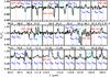 |
Fig. C.1 Close-ups of several of the H2O, CO and OH lines in W3IRS5 as shown in Fig. 1. The rest wavelength of each line is indicated by dashed lines: blue for H2O, red for CO, and light blue for OH. Identifications of the undetected lines in the presented spectral regions are shown in parenthesis. |
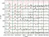 |
Fig. C.2 Close-ups of several transitions of CO lines in the PACS wavelength range toward all sources. The spectra are continuum-subtracted and shifted vertically for better visualization. |
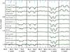 |
Fig. C.3 Normalized spectra of OH doublets for all our sources at central position. Doublets at 71 and 98 μm are excluded because of poor calibration of those spectral regions observed with PACS. OH doublet at 84.4 μm is a blend with the CO 31–30 line, whereas OH at 65.13 μm can be affected by H2O 625–514 at 65.17 μm. |
Appendix D: OH in low and intermediate mass sources
Figures D.1 and D.2 show rotational diagrams of OH for low- and intermediate-mass young stellar objects based on the fluxes presented in Wampfler et al. (2013). Only the sources with at least three detected doublets in emission (out of 4 targeted in total) are shown in diagrams. Rotational temperatures and total numbers of emitting molecules are summarized in Table D.1. For low-mass YSOs, a single component fit is usually not a good approximation (with the exception of L1527 and IRAS15398). In the intermediate-mass YSOs, on the other hand, such an approximation holds and results in very similar rotational temperatures of OH Trot ~ 35 K for all sources except NGC 7129 FIRS2.
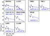 |
Fig. D.1 OH rotational diagrams (from emission lines) for low-mass young stellar objects (fluxes from Wampfler et al. 2013). |
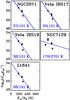 |
Fig. D.2 OH rotational diagrams (from emission lines) for intermediate-mass young stellar objects (fluxes from Wampfler et al. 2013). |
OH rotational excitation and number of emitting molecules based on emission lines for low- and intermediate-mass sources.
Herschel is an ESA space observatory with science instruments provided by European-led Principal Investigator consortia and with important participation from NASA.
The highest-excited OH doublet at 71 μm is not considered further in the analysis, because the 70–73 μm region observed with PACS is affected by spectral leakage and thus is badly flux-calibrated.
The value in the brackets (23) shows the average error of rotational temperatures for different sources, whereas ± 60 is the standard deviation of rotational temperatures.
Acknowledgments
Herschel is an ESA space observatory with science instruments provided by the European-led Principal Investigator consortia and with important participation from NASA. A.K. acknowledges support from the Christiane Nüsslein-Volhard-Foundation, the L′Oréal Deutschland, and the German Commission for UNESCO via the “Women in Science” prize. J.R.G., L.C., and J.C. thank the Spanish MINECO for funding support from grants AYA2009-07304, AYA2012-32032, and CSD2009-00038 and AYA. J.R.G. is supported by a Ramoón y Cajal research contract. Astrochemistry in Leiden is supported by the Netherlands Research School for Astronomy (NOVA), by a Royal Netherlands Academy of Arts and Sciences (KNAW) professor prize, by a Spinoza grant and grant 614.001.008 from the Netherlands Organisation for Scientific Research (NWO), and by the European Community’s Seventh Framework Program FP7/2007-2013 under grant agreement 238258 (LASSIE).
References
- André, P., Ward-Thompson, D., & Barsony, M. 1993, ApJ, 406, 122 [NASA ADS] [CrossRef] [Google Scholar]
- André, P., Ward-Thompson, D., & Barsony, M. 2000, Protostars and Planets IV, 59 [Google Scholar]
- Beuther, H., Churchwell, E. B., McKee, C. F., & Tan, J. C. 2007, Protostars and Planets V (Tucson: University of Arizona press), 165 [Google Scholar]
- Bontemps, S., Andre, P., Terebey, S., & Cabrit, S. 1996, A&A, 311, 858 [NASA ADS] [Google Scholar]
- Boonman, A. M. S., & van Dishoeck, E. F. 2003, A&A, 403, 1003 [Google Scholar]
- Boonman, A. M. S., Doty, S. D., van Dishoeck, E. F., et al. 2003, A&A, 406, 937 [NASA ADS] [CrossRef] [EDP Sciences] [Google Scholar]
- Ceccarelli, C., Hollenbach, D. J., & Tielens, A. G. G. M. 1996, ApJ, 471, 400 [Google Scholar]
- Cernicharo, J., Goicoechea, J. R., & Caux, E. 2000, ApJ, 534, L199 [NASA ADS] [CrossRef] [PubMed] [Google Scholar]
- Cernicharo, J., Goicoechea, J. R., Daniel, F., et al. 2006, ApJ, 649, L33 [NASA ADS] [CrossRef] [Google Scholar]
- Cesaroni, R. 2005, Ap&SS, 295, 5 [NASA ADS] [CrossRef] [Google Scholar]
- Chavarría, L., Herpin, F., Jacq, T., et al. 2010, A&A, 521, L37 [NASA ADS] [CrossRef] [EDP Sciences] [Google Scholar]
- Clegg, P. E., Ade, P. A. R., Armand, C., et al. 1996, A&A, 315, L38 [NASA ADS] [Google Scholar]
- Daniel, F., Dubernet, M.-L., & Grosjean, A. 2011, A&A, 536, A76 [NASA ADS] [CrossRef] [EDP Sciences] [Google Scholar]
- de Graauw, T., Haser, L. N., Beintema, D. A., et al. 1996, A&A, 315, L49 [NASA ADS] [Google Scholar]
- de Graauw, T., Helmich, F. P., Phillips, T. G., et al. 2010, A&A, 518, L6 [NASA ADS] [CrossRef] [EDP Sciences] [Google Scholar]
- Doty, S. D., & Neufeld, D. A. 1997, ApJ, 489, 122 [NASA ADS] [CrossRef] [Google Scholar]
- Fich, M., Johnstone, D., van Kempen, T. A., et al. 2010, A&A, 518, L86 [NASA ADS] [CrossRef] [EDP Sciences] [Google Scholar]
- Fischer, J., Luhman, M. L., Satyapal, S., et al. 1999, Ap&SS, 266, 91 [NASA ADS] [CrossRef] [Google Scholar]
- Goicoechea, J. R., & Cernicharo, J. 2001, ApJ, 554, L213 [NASA ADS] [CrossRef] [Google Scholar]
- Goicoechea, J. R., Cernicharo, J., Lerate, M. R., et al. 2006, ApJ, 641, L49 [NASA ADS] [CrossRef] [Google Scholar]
- Goicoechea, J. R., Cernicharo, J., Karska, A., et al. 2012, A&A, 548, A77 [NASA ADS] [CrossRef] [EDP Sciences] [Google Scholar]
- Goldsmith, P. F., & Langer, W. D. 1999, ApJ, 517, 209 [NASA ADS] [CrossRef] [Google Scholar]
- Green, J. D., Evans, II, N. J., Jørgensen, J. K., et al. 2013, ApJ, 770, 123 [NASA ADS] [CrossRef] [Google Scholar]
- Harwit, M., Neufeld, D. A., Melnick, G. J., & Kaufman, M. J. 1998, ApJ, 497, L105 [NASA ADS] [CrossRef] [Google Scholar]
- Helmich, F. P., & van Dishoeck, E. F. 1997, A&AS, 124, 205 [NASA ADS] [CrossRef] [EDP Sciences] [Google Scholar]
- Herczeg, G. J., Brown, J. M., van Dishoeck, E. F., & Pontoppidan, K. M. 2011, A&A, 533, A112 [NASA ADS] [CrossRef] [EDP Sciences] [Google Scholar]
- Herczeg, G. J., Karska, A., Bruderer, S., et al. 2012, A&A, 540, A84 [NASA ADS] [CrossRef] [EDP Sciences] [Google Scholar]
- Hogerheijde, M. R., & van der Tak, F. F. S. 2000, A&A, 362, 697 [NASA ADS] [Google Scholar]
- Karska, A., Herczeg, G. J., van Dishoeck, E. F., et al. 2013, A&A, 552, A141 [NASA ADS] [CrossRef] [EDP Sciences] [Google Scholar]
- Kessler, M. F., Steinz, J. A., Anderegg, M. E., et al. 1996, A&A, 315, L27 [NASA ADS] [Google Scholar]
- Kristensen, L. E., van Dishoeck, E. F., Bergin, E. A., et al. 2012, A&A, 542, A8 [NASA ADS] [CrossRef] [EDP Sciences] [Google Scholar]
- Lee, J., Lee, J.-E., Lee, S., et al. 2013, ApJS, 209, 4 [NASA ADS] [CrossRef] [Google Scholar]
- Leurini, S., Wyrowski, F., Herpin, F., et al. 2013, A&A, 550, A10 [NASA ADS] [CrossRef] [EDP Sciences] [Google Scholar]
- Manoj, P., Watson, D. M., Neufeld, D. A., et al. 2013, ApJ, 763, 83 [NASA ADS] [CrossRef] [Google Scholar]
- Mitchell, G. F., Maillard, J.-P., Allen, M., Beer, R., & Belcourt, K. 1990, ApJ, 363, 554 [NASA ADS] [CrossRef] [Google Scholar]
- Mottram, J. C., van Dishoeck, E. F., Schmalzl, M., et al. 2013, A&A, 558, A126 [NASA ADS] [CrossRef] [EDP Sciences] [Google Scholar]
- Neufeld, D. A. 2012, ApJ, 749, 125 [NASA ADS] [CrossRef] [Google Scholar]
- Nisini, B., Giannini, T., & Lorenzetti, D. 2002, ApJ, 574, 246 [NASA ADS] [CrossRef] [Google Scholar]
- Ott, S. 2010, in Astronomical Data Analysis Software and Systems XIX, eds. Y. Mizumoto, K.-I. Morita, & M. Ohishi, ASP Conf. Ser., 434, 139 [Google Scholar]
- Pilbratt, G. L., Riedinger, J. R., Passvogel, T., et al. 2010, A&A, 518, L1 [CrossRef] [EDP Sciences] [Google Scholar]
- Poglitsch, A., Waelkens, C., Geis, N., et al. 2010, A&A, 518, L2 [NASA ADS] [CrossRef] [EDP Sciences] [Google Scholar]
- Robitaille, T. P. 2011, A&A, 536, A79 [NASA ADS] [CrossRef] [EDP Sciences] [Google Scholar]
- Rosenthal, D., Bertoldi, F., & Drapatz, S. 2000, A&A, 356, 705 [NASA ADS] [Google Scholar]
- San José-García, I., Mottram, J. C., Kristensen, L. E., et al. 2013, A&A, 553, A125 [NASA ADS] [CrossRef] [EDP Sciences] [Google Scholar]
- Schöier, F. L., van der Tak, F. F. S., van Dishoeck, E. F., & Black, J. H. 2005, A&A, 432, 369 [NASA ADS] [CrossRef] [EDP Sciences] [Google Scholar]
- Sempere, M. J., Cernicharo, J., Lefloch, B., González-Alfonso, E., & Leeks, S. 2000, ApJ, 530, L123 [NASA ADS] [CrossRef] [Google Scholar]
- Shirley, Y. L., Evans, II, N. J., Rawlings, J. M. C., & Gregersen, E. M. 2000, ApJS, 131, 249 [NASA ADS] [CrossRef] [Google Scholar]
- Shu, F. H., Adams, F. C., & Lizano, S. 1987, ARA&A, 25, 23 [Google Scholar]
- Sturm, E., Lutz, D., Verma, A., et al. 2002, A&A, 393, 821 [NASA ADS] [CrossRef] [EDP Sciences] [Google Scholar]
- van der Tak, F. F. S., van Dishoeck, E. F., Evans, II, N. J., & Blake, G. A. 2000, ApJ, 537, 283 [NASA ADS] [CrossRef] [Google Scholar]
- van der Tak, F. F. S., Black, J. H., Schöier, F. L., Jansen, D. J., & van Dishoeck, E. F. 2007, A&A, 468, 627 [NASA ADS] [CrossRef] [EDP Sciences] [Google Scholar]
- van der Tak, F. F. S., Chavarría, L., Herpin, F., et al. 2013, A&A, 554, A83 [NASA ADS] [CrossRef] [EDP Sciences] [Google Scholar]
- van der Wiel, M. H. D., Pagani, L., van der Tak, F. F. S., Kaźmierczak, M., & Ceccarelli, C. 2013, A&A, 553, A11 [NASA ADS] [CrossRef] [EDP Sciences] [Google Scholar]
- van Dishoeck, E. F. 2004, ARA&A, 42, 119 [NASA ADS] [CrossRef] [Google Scholar]
- van Dishoeck, E. F., Wright, C. M., Cernicharo, J., et al. 1998, ApJ, 502, L173 [NASA ADS] [CrossRef] [Google Scholar]
- van Dishoeck, E. F., Kristensen, L. E., Benz, A. O., et al. 2011, PASP, 123, 138 [NASA ADS] [CrossRef] [Google Scholar]
- van Kempen, T. A., van Dishoeck, E. F., Güsten, R., et al. 2009, A&A, 501, 633 [NASA ADS] [CrossRef] [EDP Sciences] [Google Scholar]
- van Kempen, T. A., Kristensen, L. E., Herczeg, G. J., et al. 2010, A&A, 518, L121 [NASA ADS] [CrossRef] [EDP Sciences] [Google Scholar]
- Vastel, C., Spaans, M., Ceccarelli, C., Tielens, A. G. G. M., & Caux, E. 2001, A&A, 376, 1064 [NASA ADS] [CrossRef] [EDP Sciences] [Google Scholar]
- Visser, R., Kristensen, L. E., Bruderer, S., et al. 2012, A&A, 537, A55 [NASA ADS] [CrossRef] [EDP Sciences] [Google Scholar]
- Wampfler, S. F., Bruderer, S., Karska, A., et al. 2013, A&A, 552, A56 [NASA ADS] [CrossRef] [EDP Sciences] [Google Scholar]
- Whitney, B., Robitaille, T., & Bjorkman, J. 2013, ApJS, submitted [Google Scholar]
- Wilson, T. L., & Rood, R. 1994, ARA&A, 32, 191 [NASA ADS] [CrossRef] [Google Scholar]
- Wright, C. M., van Dishoeck, E. F., Black, J. H., et al. 2000, A&A, 358, 689 [NASA ADS] [Google Scholar]
- Wyrowski, F., Menten, K. M., Schilke, P., et al. 2006, A&A, 454, L91 [NASA ADS] [CrossRef] [EDP Sciences] [Google Scholar]
- Yıldız, U. A., van Dishoeck, E. F., Kristensen, L. E., et al. 2010, A&A, 521, L40 [Google Scholar]
- Yıldız, U. A., Kristensen, L. E., van Dishoeck, E. F., et al. 2012, A&A, 542, A86 [NASA ADS] [CrossRef] [EDP Sciences] [Google Scholar]
- Yıldız, U. A., Kristensen, L. E., van Dishoeck, E. F., et al. 2013, A&A, 556, A89 [NASA ADS] [CrossRef] [EDP Sciences] [Google Scholar]
- Zinnecker, H., & Yorke, H. W. 2007, ARA&A, 45, 481 [NASA ADS] [CrossRef] [Google Scholar]
All Tables
OH rotational excitation and number of emitting molecules based on emission lines for low- and intermediate-mass sources.
All Figures
|
Fig. 1 Herschel/PACS continuum-normalized spectrum of W3 IRS5 at the central position. Lines of CO are shown in red, H2O in blue, OH in light blue, CH in orange, and atoms and ions in green. Horizontal magenta lines show spectral regions zoomed in Fig. C.1. |
| In the text | |
|
Fig. 2 Herschel/PACS profiles of the [O i] 63.2 μm line at central position. |
| In the text | |
|
Fig. 3 Normalized spectral regions of all our sources at the central position at 64–68, 148–157, and 169–182 μm. Objects are shown in the evolutionary sequence, with the most evolved ones on top. Lines of CO are shown in red, H2O in blue, OH in light blue, CH in orange, and NH3 and C3 in green. Spectra are shifted vertically to improve the clarity of the figure. |
| In the text | |
|
Fig. 4 Relative contributions of [O i] (dark blue), CO (yellow), H2O (orange), and OH (red) cooling to the total far-IR gas cooling at central position are shown from left to right horizontally for each source. The objects follow the evolutionary sequence with the most evolved sources on top. |
| In the text | |
|
Fig. 5 Rotational diagrams of CO for all objects in our sample. The base-10 logarithm of the number of emitting molecules from a level u, |
| In the text | |
|
Fig. 6 Rotational diagrams of H2O calculated using emission lines (left column) and absorption lines (right column), respectively. For emission line diagrams, the logarithm with base 10 of total number of molecules in a level u, |
| In the text | |
|
Fig. 7 Rotational diagrams of H2O calculated using absorption lines. A single-component fit is used to calculate the temperature shown in the panels. |
| In the text | |
|
Fig. 8 Top: rotational diagram of H2O calculated assuming a kinetic temperature T = 1000 K, H2 density n = 106 cm-3, H2O column density 2 × 1016 cm-2, and line width ΔV = 5 km s-1. Lines observed in absorption in NGC 6334-I are shown in blue. Fits are done to all lines in the PACS range included in the LAMDA database (Schöier et al. 2005) (in black) and to the NGC 6334-I lines (in blue). Darker shades denote optically thin lines. Bottom: the same as above, but assuming an H2O column density 1012 cm-2, such that all lines are optically thin. |
| In the text | |
|
Fig. 9 Rotational diagrams of OH calculated using absorption lines, similar to Fig. 7 for H2O. The single component fit to all OH transitions detected in absorption is shown with a solid line with the corresponding temperature. A separate single component fit is done for the OH |
| In the text | |
|
Fig. 10 Top: comparison of integrated line fluxes of 12CO observed by Herschel/PACS and from the ground (black dots with errorbars) and the predictions of the quiescent envelope passively heated by the luminosity of the source (red crosses) for NGC 7538-IRS1. Bottom: the same model compared with the JCMT 12CO 3–2 and Herschel/HIFI 13CO 10–9 and C18O 9–8 observed line profiles. An additional model including an outflow component is shown in blue dashed line. |
| In the text | |
|
Fig. 11 Comparison of integrated line fluxes of CO observed by PACS only (black dots with error bars) and the predictions of the quiescent envelope passively heated by the luminosity of the source (red crosses). |
| In the text | |
|
Fig. 12 Rotational temperatures of CO, H2O, and OH for low- to high-mass star forming regions. WISH, DIGIT, and HOPS team’s results with PACS are shown in blue, red, and navy blue, respectively. Dotted lines show the median values of the rotational temperature from each database; for the case of WISH, the median is calculated separately for objects with Lbol < 103 L⊙ and Lbol > 103 L⊙, except for OH where intermediate-mass YSOs covering 103 > Lbol > 50 L⊙ are also shown separately. The CO and H2O excitation of intermediate-mass sources has not yet been surveyed with Herschel. |
| In the text | |
|
Fig. 13 Correlations of line emission with bolometric luminosity (left column) and envelope mass (right column) from top to bottom: CO 14–13, H2O 303–212, [O i] at 145 μm and OH 163 μm line luminosities. Low- and intermediate-mass young stellar objects emission is measured over 5 × 5 PACS maps. Red and blue circles show Class 0 and Class I low-mass YSOs from Karska et al. (2013). Blue diamonds show intermediate-mass YSOs from Wampfler et al. (2013; O and OH lines) and from Fich et al. (2010; CO and H2O line). High-mass YSOs fluxes are measured in the central position and shown in black. Pearson coefficient r is given for each correlation. |
| In the text | |
|
Fig. 14 From top to bottom: (1) total far-IR line cooling; (2) ratio of molecular to atomic cooling; (3) gas-to-dust cooling ratio, LFIRL/Lbol, where LFIRL = Lmol + Latom; as a function of bolometric luminosity. Low-mass YSOs are shown in red (Class 0) and blue (Class I), whereas high-mass ones are in black. |
| In the text | |
|
Fig. C.1 Close-ups of several of the H2O, CO and OH lines in W3IRS5 as shown in Fig. 1. The rest wavelength of each line is indicated by dashed lines: blue for H2O, red for CO, and light blue for OH. Identifications of the undetected lines in the presented spectral regions are shown in parenthesis. |
| In the text | |
|
Fig. C.2 Close-ups of several transitions of CO lines in the PACS wavelength range toward all sources. The spectra are continuum-subtracted and shifted vertically for better visualization. |
| In the text | |
|
Fig. C.3 Normalized spectra of OH doublets for all our sources at central position. Doublets at 71 and 98 μm are excluded because of poor calibration of those spectral regions observed with PACS. OH doublet at 84.4 μm is a blend with the CO 31–30 line, whereas OH at 65.13 μm can be affected by H2O 625–514 at 65.17 μm. |
| In the text | |
|
Fig. D.1 OH rotational diagrams (from emission lines) for low-mass young stellar objects (fluxes from Wampfler et al. 2013). |
| In the text | |
|
Fig. D.2 OH rotational diagrams (from emission lines) for intermediate-mass young stellar objects (fluxes from Wampfler et al. 2013). |
| In the text | |
Current usage metrics show cumulative count of Article Views (full-text article views including HTML views, PDF and ePub downloads, according to the available data) and Abstracts Views on Vision4Press platform.
Data correspond to usage on the plateform after 2015. The current usage metrics is available 48-96 hours after online publication and is updated daily on week days.
Initial download of the metrics may take a while.