| Issue |
A&A
Volume 561, January 2014
|
|
|---|---|---|
| Article Number | A86 | |
| Number of page(s) | 22 | |
| Section | Extragalactic astronomy | |
| DOI | https://doi.org/10.1051/0004-6361/201322217 | |
| Published online | 07 January 2014 | |
The evolution of the dust temperatures of galaxies in the SFR–M∗ plane up to z ~ 2⋆,⋆⋆
1
Max-Planck-Institut für extraterrestrische Physik,
Postfach 1312, Giessenbachstraße
1, 85741
Garching,
Germany
e-mail: This email address is being protected from spambots. You need JavaScript enabled to view it.
2
Argelander-Institut für Astronomie, University of
Bonn, auf dem Hügel
71, 53121
Bonn,
Germany
3
Department of Physics and Astronomy, University College
London, Gower
Street, London
WC1E 6BT,
UK
4
INAF – Osservatorio Astronomico di Roma,
via di Frascati 33,
00040
Monte Porzio Catone,
Italy
5
Astronomy Centre, Dept. of Physics & Astronomy, University of
Sussex, Brighton
BN1 9QH,
UK
6
Mullard Space Science Laboratory, University College
London, Holmbury St
Mary, Dorking
RH5 6NT,
UK
7
Herschel Science Centre, ESAC, Villanueva de la
Cañada, 28691
Madrid,
Spain
8
ESO, Karl-Schwarzschild-Straße 2, 85748
Garching,
Germany
9
INAF – Osservatorio Astronomico di Trieste,
via Tiepolo 11, 34143
Trieste,
Italy
10
Laboratoire AIM, CEA/DSM-CNRS-Université Paris Diderot,
IRFU/Service d’Astrophysique, Bât.709, CEA-Saclay, 91191
Gif-sur-Yvette Cedex,
France
11
California Institute of Technology, 1200 E. California Blvd., Pasadena
CA
91125,
USA
12
Jet Propulsion Laboratory, 4800 Oak Grove Drive, Pasadena
CA
91109,
USA
13
Instituto de Astrofísica de Canarias (IAC),
C/vía Láctea s/n, 38200
La Laguna,
Spain
14
Departamento de Astrofísica, Universidad de La
Laguna, 38206
La Laguna,
Spain
15
Dipartimento di Astronomia, Università di Bologna,
via Ranzani 1, 40127
Bologna,
Italy
16
Center for Astrophysics and Space Astronomy, 389 UCB, University
of Colorado, Boulder
CO
80309,
USA
17
Institute for Astronomy, University of Edinburgh, Royal
Observatory, Blackford
Hill, Edinburgh
EH9 3HJ,
UK
18
Department of Physics, University of Oxford,
Keble Road, Oxford
OX1 3RH,
UK
19
School of Physics and Astronomy, The Raymond and Beverly Sackler
Faculty of Exact Sciences, Tel Aviv University, 69978
Tel Aviv,
Israel
20
NASA Ames, Moffett Field, CA
94035,
USA
21
Dipartimento di Astronomia, Universita di Padova,
Vicolo dell’Osservatorio 3,
35122
Padova,
Italy
22
Department of Physics & Astronomy, University of British
Columbia, 6224 Agricultural
Road, Vancouver BC
V6T 1Z1,
Canada
Received:
5
July
2013
Accepted:
11
November
2013
Abstract
We study the evolution of the dust temperature of galaxies in the SFR− M∗ plane up to z ~ 2 using far-infrared and submillimetre observations from the Herschel Space Observatory taken as part of the PACS Evolutionary Probe (PEP) and Herschel Multi-tiered Extragalactic Survey (HerMES) guaranteed time key programmes. Starting from a sample of galaxies with reliable star-formation rates (SFRs), stellar masses (M∗) and redshift estimates, we grid the SFR− M∗parameter space in several redshift ranges and estimate the mean dust temperature (Tdust) of each SFR–M∗ − z bin. Dust temperatures are inferred using the stacked far-infrared flux densities (100–500 μm) of our SFR–M∗ − z bins. At all redshifts, the dust temperature of galaxies smoothly increases with rest-frame infrared luminosities (LIR), specific SFRs (SSFR; i.e., SFR/M∗), and distances with respect to the main sequence (MS) of the SFR− M∗ plane (i.e., Δlog (SSFR)MS = log [SSFR(galaxy)/SSFRMS(M∗,z)]). The Tdust − SSFR and Tdust − Δlog (SSFR)MS correlations are statistically much more significant than the Tdust − LIR one. While the slopes of these three correlations are redshift-independent, their normalisations evolve smoothly from z = 0 and z ~ 2. We convert these results into a recipe to derive Tdust from SFR, M∗ and z, valid out to z ~ 2 and for the stellar mass and SFR range covered by our stacking analysis. The existence of a strong Tdust − Δlog (SSFR)MS correlation provides us with several pieces of information on the dust and gas content of galaxies. Firstly, the slope of the Tdust − Δlog (SSFR)MS correlation can be explained by the increase in the star-formation efficiency (SFE; SFR/Mgas) with Δlog (SSFR)MS as found locally by molecular gas studies. Secondly, at fixed Δlog (SSFR)MS, the constant dust temperature observed in galaxies probing wide ranges in SFR and M∗ can be explained by an increase or decrease in the number of star-forming regions with comparable SFE enclosed in them. And thirdly, at high redshift, the normalisation towards hotter dust temperature of the Tdust − Δlog (SSFR)MS correlation can be explained by the decrease in the metallicities of galaxies or by the increase in the SFE of MS galaxies. All these results support the hypothesis that the conditions prevailing in the star-forming regions of MS and far-above-MS galaxies are different. MS galaxies have star-forming regions with low SFEs and thus cold dust, while galaxies situated far above the MS seem to be in a starbursting phase characterised by star-forming regions with high SFEs and thus hot dust.
Key words: galaxies: evolution / infrared: galaxies / galaxies: starburst
Herschel is an ESA space observatory with science instruments provided by European-led Principal Investigator consortia and with important participation from NASA.
Appendices are available in electronic form at http://www.aanda.org
© ESO, 2014
1. Introduction
Over the last 10 Gyr of lookback time, we observed a clear correlation between the star
formation rate (SFR) and the stellar mass (M∗) of star-forming
galaxies, SFR ∝  , with 0.5 < α < 1.0
(Brinchmann et al. 2004; Schiminovich et al. 2007; Noeske et al.
2007; Elbaz et al. 2007; Daddi et al. 2007; Pannella et al.(2009)Pannella Carilli; Dunne et
al. 2009; Rodighiero et al. 2010; Oliver et al. 2010; Magdis et al. 2010b; Karim et al. 2011;
Mancini et al. 2011; Whitaker et al. 2012). The existence of this so-called “main sequence”
(MS) of star formation, whose normalisation declines from z = 2.5 to 0, is
usually taken as evidence that the bulk of the star-forming galaxy (SFG) population is
evolving through a steady mode of star formation, likely sustained by the accretion of cold
gas from the intergalactic medium (IGM) or along the cosmic web (e.g., Dekel et al. 2009). In that picture, occasional major merger events
create extreme systems with intense short-lived starbursts, which are offset from the MS of
star formation (see e.g., Engel et al. 2010). One
strong observational confirmation of this interpretation is that the physical properties of
star-forming galaxies are fundamentally linked to their positions with respect to the MS of
star formation (i.e.,
Δlog (SSFR)MS = log [SSFR(galaxy)/SSFRMS(M∗,z)]).
On one hand, galaxies situated on the MS of star formation typically have a disk-like
morphology, relatively low SFR surface density (Wuyts et al.
2011b), high ratio of mid-infrared polycyclic aromatic hydrocarbon (PAHs) to
far-infrared (FIR) emission (Elbaz et al. 2011; Nordon et al. 2012), and a high C ii-to-FIR
ratio (Graciá-Carpio et al. 2011). On the other hand,
off-MS galaxies (throughout, the term “off-MS galaxies” refers to galaxies situated
above the MS) have cuspier morphology, higher SFR surface density,
smaller PAH-to-FIR ratio and C ii-to-FIR ratios. Additionally, on- and off-MS
galaxies exhibit fundamental differences in the physical conditions prevailing in their
giant molecular clouds (GMCs). MS galaxies have high CO-to-H2 conversion factors,
consistent with star-forming regions that are mainly constituted by well virialized GMCs,
while off-MS galaxies have low CO-to-H2 conversion factors, consistent with
star-forming regions being constituted by unvirialized GMCs, as observed in local major
mergers (Magnelli et al. 2012b; Genzel et al. 2010; Daddi et al.
2010; Magdis et al. 2012).
, with 0.5 < α < 1.0
(Brinchmann et al. 2004; Schiminovich et al. 2007; Noeske et al.
2007; Elbaz et al. 2007; Daddi et al. 2007; Pannella et al.(2009)Pannella Carilli; Dunne et
al. 2009; Rodighiero et al. 2010; Oliver et al. 2010; Magdis et al. 2010b; Karim et al. 2011;
Mancini et al. 2011; Whitaker et al. 2012). The existence of this so-called “main sequence”
(MS) of star formation, whose normalisation declines from z = 2.5 to 0, is
usually taken as evidence that the bulk of the star-forming galaxy (SFG) population is
evolving through a steady mode of star formation, likely sustained by the accretion of cold
gas from the intergalactic medium (IGM) or along the cosmic web (e.g., Dekel et al. 2009). In that picture, occasional major merger events
create extreme systems with intense short-lived starbursts, which are offset from the MS of
star formation (see e.g., Engel et al. 2010). One
strong observational confirmation of this interpretation is that the physical properties of
star-forming galaxies are fundamentally linked to their positions with respect to the MS of
star formation (i.e.,
Δlog (SSFR)MS = log [SSFR(galaxy)/SSFRMS(M∗,z)]).
On one hand, galaxies situated on the MS of star formation typically have a disk-like
morphology, relatively low SFR surface density (Wuyts et al.
2011b), high ratio of mid-infrared polycyclic aromatic hydrocarbon (PAHs) to
far-infrared (FIR) emission (Elbaz et al. 2011; Nordon et al. 2012), and a high C ii-to-FIR
ratio (Graciá-Carpio et al. 2011). On the other hand,
off-MS galaxies (throughout, the term “off-MS galaxies” refers to galaxies situated
above the MS) have cuspier morphology, higher SFR surface density,
smaller PAH-to-FIR ratio and C ii-to-FIR ratios. Additionally, on- and off-MS
galaxies exhibit fundamental differences in the physical conditions prevailing in their
giant molecular clouds (GMCs). MS galaxies have high CO-to-H2 conversion factors,
consistent with star-forming regions that are mainly constituted by well virialized GMCs,
while off-MS galaxies have low CO-to-H2 conversion factors, consistent with
star-forming regions being constituted by unvirialized GMCs, as observed in local major
mergers (Magnelli et al. 2012b; Genzel et al. 2010; Daddi et al.
2010; Magdis et al. 2012).
The task at hand is now to confirm this interpretation of on- and above-MS galaxies, but also to understand the evolutionary scenario linking this population of star-forming galaxies with the large population of massive (i.e., M∗ > 1010.5 M⊙) and passive (i.e., SFR < 1 M⊙ yr-1) galaxies constituting the “red sequence” of the optical colour-magnitude diagram (e.g., Baldry et al. 2004; Faber et al. 2007), and which exists over the full redshift range covered by our study (Fontana et al. 2009).
In this context, we study here the evolution of the dust temperature (Tdust) of galaxies in the SFR− M∗ plane up to z ~ 2. Such an analysis is crucial, because estimates of Tdust provide us with information on the physical conditions prevailing in the star-forming regions of galaxies. In particular, because there is a link between Tdust, the radiation field, dust and gas content (via the gas-to-dust ratio), the existence of a positive correlation between dust temperature and Δlog (SSFR)MS would give strong support to the usual interpretation of the MS of star formation. Indeed, MS galaxies with their low SFR surface densities and star-formation efficiencies (SFE, i.e., SFR/Mgas; Saintonge et al. 2012) should have relatively low dust temperatures, while off-MS galaxies with their high SFR surface densities and SFEs should have hotter dust temperatures. In addition, we note that studying variations of the dust temperature in the SFR− M∗ plane is also important to test the accuracy of FIR spectral energy distribution (SED) libraries routinely used to infer total infrared luminosities from monochromatic observations, or used in backward evolutionary models (see e.g., Valiante et al. 2009; Béthermin et al. 2012a).
Estimating Tdust for a large sample of galaxies up to zs2 was only made possible by the Herschel Space Observatory (Pilbratt et al. 2010). With the Photodetector Array Camera and Spectrometer (PACS; Poglitsch et al. 2010) instrument and the Spectral and Photometric Imaging REceiver (SPIRE; Griffin et al. 2010), it is possible to probe the peak of the rest frame FIR/submillimetre emission of galaxies. Here, we use the deepest PACS and SPIRE observations obtained as part of the PACS Evolutionary Probe (PEP1; Lutz et al. 2011) and the Herschel Multi-tiered Extragalactic Survey (HerMES2; Oliver et al. 2012) guaranteed time key programmes covering an area of s 2.0 deg2. The combination of these PACS and SPIRE observations, together with a careful stacking analysis, provide a very powerful tool to study the FIR/submillimetre SEDs of high-redshift galaxies. In particular, we are able to grid the SFR− M∗ plane in several redshift bins, extending up to zs2, and to estimate the dust temperature of each SFR–M∗ − z bin. Based on these estimates, we study the correlation between the dust temperature of galaxies and their infrared luminosities (see also Symeonidis et al. 2013), specific SFRs (SSFR, i.e., SFR/M∗) and their distances with respect to MS of star formation. Then, using a simple model to link Tdust with the dust and gas content of galaxies, we ascribe these correlations to variations in the physical conditions prevailing in their star-forming regions.
The paper is structured as follows. In Sect. 2 we present the Herschel data and the multi-wavelength sample used in our study. Section 3 presents the method used to infer the evolution of the dust temperature in the SFR− M∗ plane from individual detections and a careful stacking analysis. We discuss the selection function of our sample in Sect. 4.1 and present the variation of the dust temperature in the SFR− M∗ plane in Sect. 4.2. Results3 are discussed in Sect. 5. Finally, we summarise our findings in Sect. 6.
Throughout the paper we use a cosmology with H0 = 71 km s-1 Mpc-1, ΩΛ = 0.73 and ΩM = 0.27. A Chabrier (2003) initial mass function (IMF) is always assumed.
2. Data
2.1. Herschel observations
In order to derive the dust temperature of our galaxies, we use deep PACS 100 and 160 μm and SPIRE 250, 350 and 500 μm observations provided by the Herschel Space Observatory. PACS observations were taken as part of the PEP (Lutz et al. 2011) guaranteed time key programme, while the SPIRE observations were taken as part of the Herschel Multi-tiered Extragalactic Survey (HerMES; Oliver et al. 2012). The combination of these two sets of observations provides a unique and powerful tool to study the FIR SEDs of galaxies. The PEP and HerMES surveys and data reduction methods are described in Lutz et al. (2011) and Oliver et al. (2012), respectively. Here, we only summarise the properties relevant for our study.
From the PEP and HerMES programmes, we used the observations of the Great Observatories Origins Deep Survey-North (GOODS-N) and -South (GOODS-S) fields and the Cosmological evolution survey (COSMOS) field. Herschel flux densities were derived with a point-spread-function-fitting analysis, guided using the position of sources detected in deep 24 μm observations from the Multiband Imaging Photometer (MIPS; Rieke et al. 2004) on board the Spitzer Space Observatory. This method has the advantage that it deals in large part with the blending issues encountered in dense fields and provides a straightforward association between MIPS, PACS and SPIRE sources as well as with the IRAC (Infrared Array Camera) sources from which the MIPS-24 μm catalogues were constructed (Magnelli et al. 2011; Le Floc’h et al. 2009). This MIPS-24 μm-guided extraction is reliable because it has been shown that, even in the deepest PACS/SPIRE field, our MIPS-24 μm catalogues are deep enough to contain almost all PACS/SPIRE sources (Magdis et al. 2011; Lutz et al. 2011; Roseboom et al. 2010; Béthermin et al. 2012b).
In PEP, prior source extraction was performed using the method presented in Magnelli et al. (2009), while in HerMES it was performed using the method presented in Roseboom et al. (2010), both consortia using consistent MIPS-24 μm catalogues. In GOODS-N and -S, we used the GOODS MIPS-24 μm catalogue presented in Magnelli et al. (2009, 2011) reaching a 3σ limit of 20 μJy. In COSMOS, we used the deepest MIPS-24 μm catalogue available, reaching a 3σ limit of 45 μJy (Le Floc’h et al. 2009). The reliability, completeness and contamination of our PACS and SPIRE catalogues were tested via Monte-Carlo simulations. All these properties are given in Berta et al. (2011) and Roseboom et al. (2010, see also Lutz et al. 2011; and Oliver et al. 2012. Table 1 summarises the depths of the PACS and SPIRE catalogues in each of the three fields.
Our IRAC-MIPS-PACS-SPIRE catalogues were cross-matched with our multi-wavelength catalogues (Sect. 2.2), using their IRAC positions and a matching radius of 1′′.
Main properties of the PEP/HerMES fields used in this study.
2.2. Multi-wavelength observations
In this study we make extensive use of the large wealth of multi-wavelength observations available for the GOODS-N/S and COSMOS fields. The full set of multi-wavelength data used in our study is described in Wuyts et al. (2011a,b). Here, we only summarise the properties relevant for our study.
In the COSMOS field, we used the public multi-wavelength photometry described in Ilbert et al. (2009) and Gabasch et al. (2008). These catalogues provide photometry in a total of 36 medium and broad bands covering the SEDs from GALEX to IRAC wavelengths. In order to obtain reliable photometric redshifts, stellar masses and SFRs, we restricted these catalogues to i < 25 (Wuyts et al. 2011b) and to sources not flagged as problematic in the catalogue of Ilbert et al. (2009, i.e., mostly excluding objects which are nearby bright stars). To identify X-ray AGN we used the XMM-Newton catalogue released by Cappelluti et al. (2009). Finally, this multi-wavelength catalogue was restricted to the COSMOS area covered by our deep MIPS-PACS-SPIRE catalogue. This leads to an effective area of 1.9 deg2.
In the GOODS-S field we used the Ks (<24.3, 5σ) selected FIREWORKS catalogue of Wuyts et al. (2008), which provides photometry in 16 bands from U to IRAC wavelengths. X-ray observations were taken from the Chandra 2-Ms source catalogue of Luo et al. (2008). In the common region covered by our deep MIPS-PACS-SPIRE observations, our GOODS-S multi-wavelength catalogue covers an effective area of 132 arcmin2.
The GOODS-N field also benefits from extensive multi-wavelength coverage. A z+K selected PSF-matched catalogue was created for GOODS-N as part of the PEP survey4 (Berta et al. 2010, 2011), with photometry in 16 bands from GALEX to IRAC wavelengths, and a collection of spectroscopic redshifts (mainly from Barger et al. 2008). For uniformity with the GOODS-S catalogue, we restrict our analysis in GOODS-N to sources with Ks < 24.3 (3σ). We complemented this multi-wavelength catalogue with the X-ray Chandra 2-Ms catalogue of Alexander et al. (2003). In the common region covered by our deep MIPS-PACS-SPIRE observations, our GOODS-N multi-wavelength catalogue covers an effective area of 144 arcmin2.
2.3. Spectroscopic and photometric redshifts
We use spectroscopic redshifts coming from a combination of various studies (Cohen et al. 2000; Wirth et al. 2004; Cowie et al. 2004; Le Fèvre et al. 2004; Mignoli et al. 2005; Vanzella et al. 2006; Reddy et al. 2006; Barger et al. 2008; Cimatti et al. 2008; Lilly et al. 2009). For sources with no spectroscopic redshifts, we instead use photometric redshift estimates. Photometric redshifts were computed using EAZY (Brammer et al. 2008) and all optical and near infrared data available. The quality of our photometric redshifts was tested by comparing them with the spectroscopic redshifts of spectroscopically confirmed galaxies. The median and scatter of Δz/(1 + z) are (− 0.001; 0.015) at z < 1.5 and (− 0.007; 0.052) at z > 1.5. Full details are presented in Wuyts et al. (2011a,b).
2.4. Stellar masses
Stellar masses were calculated by fitting all photometric data with
 m
to Bruzual & Charlot (2003) templates using
FAST (Fitting and Assessment of Synthetic Templates; Kriek et al. 2009). The rest-frame template error function of Brammer et al. (2008) was also used to down-weight data points with
m
to Bruzual & Charlot (2003) templates using
FAST (Fitting and Assessment of Synthetic Templates; Kriek et al. 2009). The rest-frame template error function of Brammer et al. (2008) was also used to down-weight data points with
 m.
In addition, we used prescriptions from Wuyts et al.
(2011b) limiting the Bruzual & Charlot
(2003) templates to models with exponentially declining star-formation histories
and a minimum e-folding time of 300 Myr. This allows for a much better
agreement between SFRs derived from optical-to-near-infrared SED fits and those derived
using mid/FIR observations. Full details are given in Wuyts et al. (2011a,b).
m.
In addition, we used prescriptions from Wuyts et al.
(2011b) limiting the Bruzual & Charlot
(2003) templates to models with exponentially declining star-formation histories
and a minimum e-folding time of 300 Myr. This allows for a much better
agreement between SFRs derived from optical-to-near-infrared SED fits and those derived
using mid/FIR observations. Full details are given in Wuyts et al. (2011a,b).
2.5. Final sample
Our final sample is Ks-selected in GOODS-N (Ks < 24.3, down to a 3σ significance) and GOODS-S (Ks < 24.3, down to a 5σ significance) but is i-selected in COSMOS (i < 25, down to a 3σ significance). The choice of a i-selected sample for COSMOS was driven by the properties of the observations publicly available for this field. Indeed, the K-selected COSMOS catalogue of McCracken et al. (2010) is relatively shallow (i.e., Ks < 23) and is almost fully included in the deep i-selected catalogue used here (McCracken et al. 2010).
Our three multi-wavelength catalogues are not homogeneously selected and not uniform in depth, which naturally translates into different completeness limits in the SFR− M∗ plane. This incompleteness could prevent us from drawing strong conclusions on the absolute number density of sources in a given SFR− M∗ bin and could also jeopardise the characterisation of their FIR properties. However, we decided here not to apply complex and very uncertain incompleteness corrections for the following reasons.
In the GOODS fields, the selection wavelength of our multi-wavelength catalogues, the Ks band, nearly translates into pure mass completeness limits. Ilbert et al. (2013) have studied the mass completeness limits of a Ks-selected sample with a magnitude limit of Ks = 24. They found that, up to z ~ 2, such sample was complete down to M∗ = 1010 M⊙. Therefore, we conclude that with a selection limit of Ks < 24.3, our deep GOODS samples should provide us with a complete sample of galaxies with M∗ > 1010 M⊙ and up to z ~ 2. In the COSMOS field, the situation is somehow different because the selection wavelength, the i-band, does not translate into pure mass completeness limits. In a given SFR− M∗ bin, dusty systems will have fainter i-band magnitudes than unobscured systems, and will be more easily missed by our sample. In this case, the source of incompleteness might correlate with the FIR properties of galaxies and thus bias our results. Wuyts et al. (2011b) studied the region of the SFR− M∗ plane strongly affected by incompleteness in the COSMOS i < 25 catalogue. They used an ultradeep WFC3-selected catalogue of the GOODS-S field (down to H = 27), and looked at the fraction of galaxies in a given SFR− M∗ bin that had i < 25 (see Fig. 10 of Wuyts et al. 2011b). At M∗ > 1010 M⊙ (i.e., the mass range of interest of our study; see Sect. 4.1), they found that the COSMOS i < 25 selected catalogue is affected by incompleteness only at z > 1.5 and that these large incompleteness mainly affect passive galaxies (completeness < 30%) and not the SFGs situated on and above the MS of star formation (completeness > 60%). From this analysis, we conclude that up to z ~ 1.5 and for M∗ > 1010 M⊙, incompleteness in SFR− M∗ bins should not bias the characterisation of their FIR properties. At z > 1.5 and M∗ > 1010 M⊙, incompleteness in the COSMOS field becomes more problematic but should not significantly affect the FIR properties of SFR− M∗ bins situated on or above the MS of star formation. We nonetheless verified that our results are reproduced when limiting our analysis to the GOODS fields (Appendix B).
Our final sample contains 8 846, 4 753 and 254 749 sources in the GOODS-N, GOODS-S5 and COSMOS fields, respectively. Of these sources, 29%, 26% and 3% have a spectroscopic redshift, the rest photometric redshift estimates. Because we study here the dust properties of galaxies, most of our results rely on the subset of sources with mid/FIR detections. In GOODS-N, GOODS-S and COSMOS, 19%, 28% and 12% of the galaxies have mid- or FIR detections, respectively. Among those sources, 60%, 45% and 11% have a spectroscopic redshift.
2.6. Star-formation rates
We take advantage of the cross-calibrated “ladder of SFR indicators” established in Wuyts et al. (2011a) and used in Wuyts et al. (2011b). This “ladder of SFR indicators” has the advantage of taking the best SFR indicator available for a given galaxy, and establishes a consistent scale across all these indicators. This “ladder” consists of three components: first, a step where galaxies are detected both in the rest-frame UV and the FIR wavelengths covered by the PACS/SPIRE Herschel observations; second, a step where galaxies are detected both in the rest-frame UV and the mid-infrared wavelengths (i.e., in the MIPS-24 μm passband) but are undetected in the FIR; third, a step where galaxies are only detected in the rest-frame UV to near infrared wavelengths. In our final sample, 7216, 26 727 and 234 405 sources are in the first, second and third steps of the “ladder of SFR indicators”.
For galaxies with no infrared detection (i.e., galaxies of the third step), we used the SFRs estimated from the best fits obtained with FAST (see Sect. 2.4). In the regime where reference SFRUV + IR are available, these SED-modelled SFRs are fully consistent with those SFRUV+IR estimates (Wuyts et al. 2011a).
For the first and second steps, SFRs were estimated by combining the unobscured and
re-emitted emission from young stars. This was done following Kennicutt (1998) and adopting a Chabrier (2003) IMF: ![Mathematical equation: \begin{equation} \label{eq: kennicutt} {\it SFR}_{\rm UV+IR}[M_{\odot}\,{\rm yr}^{-1}]=1.09\times10^{-10}\,(L_{{\rm IR}}[L_{\odot}]+3.3\times L_{2800}[L_{\odot}]), \end{equation}](/articles/aa/full_html/2014/01/aa22217-13/aa22217-13-eq83.png) (1)where
L2800 ≡ νLν(2800 Å)
is computed with FAST from the best-fitting SED (see Sect. 2.4) and the rest-frame infrared luminosity
LIR ≡ L(8 − 1000 μm) is
derived from our mid/FIR observations. For galaxies with FIR detections,
LIR was inferred by fitting their FIR flux densities (i.e.,
PACS and SPIRE) with the SED template library of Dale
& Helou (2002, DH), leaving the normalisation of each SED template as a free
parameter. Examples of these fits are given in Fig. A.1. We note that using the SED template library of Chary & Elbaz (2001) instead of that of DH to derive
LIR (again leaving the normalisation as a free parameter),
has no impact on our results. Indeed, the
(1)where
L2800 ≡ νLν(2800 Å)
is computed with FAST from the best-fitting SED (see Sect. 2.4) and the rest-frame infrared luminosity
LIR ≡ L(8 − 1000 μm) is
derived from our mid/FIR observations. For galaxies with FIR detections,
LIR was inferred by fitting their FIR flux densities (i.e.,
PACS and SPIRE) with the SED template library of Dale
& Helou (2002, DH), leaving the normalisation of each SED template as a free
parameter. Examples of these fits are given in Fig. A.1. We note that using the SED template library of Chary & Elbaz (2001) instead of that of DH to derive
LIR (again leaving the normalisation as a free parameter),
has no impact on our results. Indeed, the  /
/ distribution has a mean value of 1 and a
dispersion of 13%. The infrared luminosity of galaxies with only a mid-infrared detection
was derived by scaling the SED template of MS galaxies (Elbaz et al. 2011) to their MIPS-24 μm flux densities. This
specific SED template was chosen because it provides good
24 μm-to-LIR conversions over a broad
range of redshifts for the vast majority of star-forming galaxies (i.e., the MS galaxies;
Elbaz et al. 2011). Figure 1 shows the localisation on the SFR–M∗ plane
of galaxies with FIR+UV, mid-infrared+UV and UV-only detections (i.e., galaxies from the
first, second and third step of the ladder, respectively). At
M∗ > 1010 M⊙,
galaxies with only mid-infrared+UV detections are mostly situated on or below the MS of
star formation. For these galaxies, the use of a
24 μm-to-LIR conversion based on the SED
template of MS galaxies should thus be a fairly good approximation. To further check the
quality of this approximation, we verified that in all SFR− M∗
bins analysed here, the mean infrared luminosities inferred from our FIR stacking analysis
(see Sect. 3.2) agrees within 0.3 dex with those
inferred from our “ladder of SFR indicators”.
distribution has a mean value of 1 and a
dispersion of 13%. The infrared luminosity of galaxies with only a mid-infrared detection
was derived by scaling the SED template of MS galaxies (Elbaz et al. 2011) to their MIPS-24 μm flux densities. This
specific SED template was chosen because it provides good
24 μm-to-LIR conversions over a broad
range of redshifts for the vast majority of star-forming galaxies (i.e., the MS galaxies;
Elbaz et al. 2011). Figure 1 shows the localisation on the SFR–M∗ plane
of galaxies with FIR+UV, mid-infrared+UV and UV-only detections (i.e., galaxies from the
first, second and third step of the ladder, respectively). At
M∗ > 1010 M⊙,
galaxies with only mid-infrared+UV detections are mostly situated on or below the MS of
star formation. For these galaxies, the use of a
24 μm-to-LIR conversion based on the SED
template of MS galaxies should thus be a fairly good approximation. To further check the
quality of this approximation, we verified that in all SFR− M∗
bins analysed here, the mean infrared luminosities inferred from our FIR stacking analysis
(see Sect. 3.2) agrees within 0.3 dex with those
inferred from our “ladder of SFR indicators”.
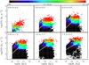 |
Fig. 1 Type of SFR indicator used in each SFR− M∗ bin. Red colours correspond to SFR− M∗ bins in which all galaxies have a FIR (i.e., PACS/SPIRE) detection, i.e., galaxies of the first step of the “ladder of SFR indicator”. Green colours correspond to SFR− M∗ bins in which galaxies are not detected in the FIR but are detected in the mid-infrared, i.e., galaxies of the second step of the “ladder of SFR indicator”. Black colours correspond to SFR− M∗ bins in which galaxies are only detected in the optical/near-infrared, i.e., galaxies of the third step of the “ladder of SFR indicator”. Short-dashed lines on a white background show the MS of star formation (see Sect. 2.7). |
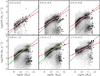 |
Fig. 2 Number density of sources in the SFR− M∗ plane. Shadings are independent for each stellar mass bin, i.e., the darkest colour indicates the highest number density of sources in the stellar mass bin and not the highest number density of sources in the entire SFR− M∗ plane. Short-dashed lines on a white background show the second order polynomial function fitted to MS of star formation (see text for details). Dotted lines present the MS found in Elbaz et al. (2011). The red triple-dot-dashed lines represent the MS found in Rodighiero et al. (2010). The green dot-dashed lines in the 0.8 < z < 1.2 and 1.2 < z < 1.7 panels show the MS found in Whitaker et al. (2012) at z ~ 1.25. |
2.7. The main sequence of star formation
Figure 2 shows the number density of sources in the SFR− M∗ plane. At M∗ < 1011 M⊙, we observe that in a given stellar mass bin, most of the galaxies have the same SFR and this characteristic SFR increases with stellar mass. In contrast, at M∗ > 1011 M⊙, SFRs seems to follow a bimodal distribution; with high SFRs extending the SFR− M∗ correlation observed at low stellar masses, and low SFRs forming a “cloud” situated far below this correlation. This bimodal distribution echoes that observed in the optical colour-magnitude diagram (e.g., Baldry et al. 2004; Faber et al. 2007), galaxies with low SFRs corresponding to galaxies from the “red sequence”, and galaxies with high SFRs corresponding to galaxies from the “blue cloud”. Focusing our attention on galaxies with relatively high SFRs, we note that over a large range of stellar masses (i.e., 109 < M∗ [M⊙] < 1011), they follow a clear SFR− M∗ correlation. This correlation is called “the main sequence” (MS) of star formation (Noeske et al. 2007).
At M∗ > 1010 M⊙, there is a good agreement between the MS observed in our sample and those inferred by Rodighiero et al. (2010) or Elbaz et al. (2011). However, taking into account the full range of stellar masses available, we observe a significant difference between our MS and those of Rodighiero et al. (2010) or Elbaz et al. (2011): the slopes of our main sequences change with stellar mass. Such a curved MS, not well described by a simple power-law function, has also been observed at z ~ 1.25 by Whitaker et al. (2012). Their main sequence, fitted with a second order polynomial function, agrees with that observed in our sample. Whitaker et al. (2012) argue that the change in the slope of the MS at high stellar masses also corresponds to a change in the intrinsic properties of the galaxies: at high stellar masses, sources are more dust rich and follow a different MS slope than lower mass galaxies with less extinction (traced by the LIR/LUV ratio).
At high stellar masses
(M∗ > 1010 M⊙),
where our results are focused, the slight disagreements observed between our MS and those
from the literature could come from several types of uncertainties and/or selection biases
(see, e.g., Karim et al. 2011). To study all these
uncertainties and selection biases is beyond the scope of this paper. Nevertheless,
because we want to investigate variations of the FIR SED properties of galaxies in the
SFR− M∗ plane, we need to precisely define the localisation
of the MS of star formation in each redshift bin. To be self-consistent, we derived the
localisation of the MS using our sample. In each redshift bin we proceeded as follows: (i)
we fitted a Gaussian function to the log (SFR) distribution of sources in each stellar
mass bin. To avoid being affected by passive galaxies, we excluded from the fit all
galaxies with  , where
 and
and
 are the localisation and dispersion of the
MS in the next lowest stellar mass bin, respectively. (ii) The localisation of the peak
and the FWHM of the Gaussian function were then defined as being, respectively, the
localisation (i.e., SFR
are the localisation and dispersion of the
MS in the next lowest stellar mass bin, respectively. (ii) The localisation of the peak
and the FWHM of the Gaussian function were then defined as being, respectively, the
localisation (i.e., SFR ) and the dispersion (i.e.,
 ) of the MS in this stellar mass bin. (iii)
We fitted the peak and dispersion of the MS in every stellar mass bin with a second order
polynomial function. Results of these fits are shown in Fig. 2 and are summarised in Table 2. In the
rest of the paper these lines are used as the MS of star formation. We note that the
typical dispersion around these best fits is ~0.3 dex, in agreement with previous
estimates of the width of the MS of star formation (e.g., Noeske et al. 2007).
) of the MS in this stellar mass bin. (iii)
We fitted the peak and dispersion of the MS in every stellar mass bin with a second order
polynomial function. Results of these fits are shown in Fig. 2 and are summarised in Table 2. In the
rest of the paper these lines are used as the MS of star formation. We note that the
typical dispersion around these best fits is ~0.3 dex, in agreement with previous
estimates of the width of the MS of star formation (e.g., Noeske et al. 2007).
Main sequence parameters.
Because there is a good overall agreement between our fits and those from the literature at M∗ > 1010 M⊙, the main results of our paper are essentially unchanged if using the MS defined by Elbaz et al. (2011, see Appendix C. However, at M∗ < 1010 M⊙, our fits significantly differ from the very steep MS defined by Elbaz et al. (2011). Although our results seem to be confirmed by Whitaker et al. (2012), further investigations will be required in this stellar mass range.
3. Data analysis
3.1. Dust temperatures
In order to obtain a proxy on the dust temperature of a galaxy, one can fit its
PACS/SPIRE flux densities with a single modified blackbody function using the optically
thin approximation: 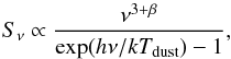 (2)where
Sν is the flux density,
β is the dust emissivity spectral index and
Tdust is the dust temperature. However, we decided not to
use this method for two reasons. Firstly, a single modified blackbody model cannot fully
describe the Wien side of the FIR SED of galaxies, because short wavelength observations
are dominated by warmer or transiently heated dust components. Therefore, one would have
to exclude from this fitting procedure all flux measurements with, for example,
λrest < 50 μm (see e.g., Hwang et al. 2010; Magnelli et al. 2012a). At high-redshift (e.g., z > 1.0),
the exclusion of some valuable flux measurements (e.g., PACS-100 μm)
would lead to an un-optimised use of our PACS/SPIRE observations. Secondly, while the
exclusion of short wavelengths would prevent the fits from being strongly biased by hot
dust components, this sharp rest-frame cut would potentially introduce a redshift
dependent bias in our dust temperature estimates. Indeed, depending on the redshift of the
source, the shortest wavelength kept in the fitting procedure (i.e., with
λrest > 50 μm) would be close, or very
close, to the wavelength cut, in which case the derived dust temperature would be
affected, or strongly affected, by hotter dust components. In the analysis done in this
paper this effect would result in an artificial increase in
Tdust with redshift of up to ~8 K.
(2)where
Sν is the flux density,
β is the dust emissivity spectral index and
Tdust is the dust temperature. However, we decided not to
use this method for two reasons. Firstly, a single modified blackbody model cannot fully
describe the Wien side of the FIR SED of galaxies, because short wavelength observations
are dominated by warmer or transiently heated dust components. Therefore, one would have
to exclude from this fitting procedure all flux measurements with, for example,
λrest < 50 μm (see e.g., Hwang et al. 2010; Magnelli et al. 2012a). At high-redshift (e.g., z > 1.0),
the exclusion of some valuable flux measurements (e.g., PACS-100 μm)
would lead to an un-optimised use of our PACS/SPIRE observations. Secondly, while the
exclusion of short wavelengths would prevent the fits from being strongly biased by hot
dust components, this sharp rest-frame cut would potentially introduce a redshift
dependent bias in our dust temperature estimates. Indeed, depending on the redshift of the
source, the shortest wavelength kept in the fitting procedure (i.e., with
λrest > 50 μm) would be close, or very
close, to the wavelength cut, in which case the derived dust temperature would be
affected, or strongly affected, by hotter dust components. In the analysis done in this
paper this effect would result in an artificial increase in
Tdust with redshift of up to ~8 K.
For these reasons, we derived the dust temperature of a galaxy using a different approach. (i) We assigned a dust temperature to each DH SED templates by fitting their z = 0 simulated PACS/SPIRE flux densities with a single modified blackbody function (see Eq. (2)). (ii) We searched for the DH SED template best-fitting the observed PACS/SPIRE flux densities of the galaxy. (iii) The dust temperature of this galaxy was then defined as being the dust temperature assigned to the corresponding DH SED template. This method makes an optimal use of our PACS/SPIRE observations and does not introduce any redshift biases. We also note that this method introduces a self-consistency between our dust temperature and infrared luminosity estimates for galaxies in the first step of the “ladder of SFR indicators” (see Sect. 2.6). Indeed both estimates are inferred using the DH SED templates best-fitting their PACS/SPIRE flux densities.
To fit the simulated z = 0 PACS/SPIRE flux densities of the DH SED templates with a modified blackbody function (i.e., step (i)), we fixed β = 1.5 and used a standard χ2 minimisation method. Results of these fits are provided in Table A.1. We note that using β = 1.5 systematically leads to higher dust temperatures than if using β = 2.0 (i.e., ΔTdust s 4 K). This Tdust − β degeneracy further highlights the limits of a single modified blackbody model in which one has to assume, or fit, an effective dust emissivity. Here, we fixed β = 1.5 because it will provide fair comparisons with most high-redshift studies in which the lack of (sub)mm observations does not allow clear constraints on β and in which the effective dust emissivity is usually fixed to 1.5 (e.g., Magdis et al. 2010a; Chapman et al. 2010; Magnelli et al. 2010, 2012a). We note that leaving β as a free parameter in our fitting procedure leads, qualitatively and quantitatively, to nearly the same Tdust − Δlog (SSFR)MS, Tdust–SSFR and Tdust − LIR relations (Sect. 4.2). However, due to this limitation, we stress that the absolute values of our dust temperature estimates should not be over-interpreted.
To fit the observed PACS/SPIRE flux densities of a galaxy with the DH SED templates
(i.e., step (ii)), we used a standard χ2 minimisation method.
Examples of such fits are given in Fig. A.1. The
dust temperature of a galaxy was then defined as being the mean dust temperature assigned
to the DH SED templates satisfying  , and from which we also defined the
1σ uncertainties. This definition symmetrises our errors bars. We note,
however, that defining the dust temperatures as the best-fit point (i.e., where
, and from which we also defined the
1σ uncertainties. This definition symmetrises our errors bars. We note,
however, that defining the dust temperatures as the best-fit point (i.e., where
 ) does not change our results.
To ensure that our dust temperature estimates are based on reliable fits and well-sampled FIR SEDs, we used three criteria:
-
the reduced χ2 should be lower than 3 (i.e., typically, χ2 < 6 for Ndof = 2).
-
there were at least 3 PACS/SPIRE data points with S/N > 3 to be fitted.
-
PACS/SPIRE data points with S/N > 3 should encompass the peak of the fitted DH SED templates.
3.2. Stacking
In order to probe the dust temperature of galaxies below the SFR completeness limit of our PACS/SPIRE observations we used a stacking analysis. This allows us to obtain the mean flux density of an individually undetected galaxy population by increasing their effective integration time using their stacked images.
3.2.1. The stacking method
Later in this paper, we demonstrate on direct detections (see Sect. 4) that the main parameter controlling the FIR
properties of galaxies is their localisation in the SFR− M∗
plane. Consequently, the most suitable way to obtain meaningful results for our stacking
analysis is to separate galaxies in different SFR–M∗ bins.
For each redshift bin, our stacking analysis was thus made as follows. First, we gridded
the SFR− M∗ plane. The size of the
SFR− M∗ grid was optimised to obtain the best balance
between a large enough number of sources per grid cell to improve the noise in the
stacked stamps ( ), and a fine enough grid to meaningfully
sample the SFR− M∗ plane. Then, for each Herschel
band (100, 160, 250, 350 and 500 μm), we stacked all
undetected galaxies in a given SFR− M∗ bin using the
residual images6. Because our galaxy sample was
drawn from fields with different PACS/SPIRE depths, the stacked image of each galaxy was
weighted by the RMS map of our observations at the position of the source. Finally, the
flux density was measured in each stacked image using the PSF-fitting method described
in Sect. 2.1. The mean flux density
(Fbin) of the SFR− M∗ bin was
then computed combining the fluxes of undetected and detected sources:
), and a fine enough grid to meaningfully
sample the SFR− M∗ plane. Then, for each Herschel
band (100, 160, 250, 350 and 500 μm), we stacked all
undetected galaxies in a given SFR− M∗ bin using the
residual images6. Because our galaxy sample was
drawn from fields with different PACS/SPIRE depths, the stacked image of each galaxy was
weighted by the RMS map of our observations at the position of the source. Finally, the
flux density was measured in each stacked image using the PSF-fitting method described
in Sect. 2.1. The mean flux density
(Fbin) of the SFR− M∗ bin was
then computed combining the fluxes of undetected and detected sources: 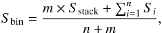 (3)where Sstack is
the stacked flux density of the m undetected sources within the
SFR− M∗ bin in the specific Herschel
band, and Si is the flux density
of the ith detected source (out of a total of n)
within the SFR− M∗ bin.
(3)where Sstack is
the stacked flux density of the m undetected sources within the
SFR− M∗ bin in the specific Herschel
band, and Si is the flux density
of the ith detected source (out of a total of n)
within the SFR− M∗ bin.
The uncertainty of the mean flux density of a given SFR− M∗ bin was computed using a standard bootstrap analysis among detections and non-detections. Allowing for repetitions, we randomly chose (n + m) sources among detections and non-detections in a given SFR− M∗ bin and computed their mean flux density. This was repeated 100 times and the flux uncertainty of the SFR− M∗ bin was defined as the standard deviation of these 100 flux densities. This uncertainty has the advantage of taking into account both measurement errors and the dispersion in the galaxy population.
From the mean PACS/SPIRE flux densities in each SFR–M∗ bin we derived a mean dust temperature using the same procedure as for galaxies with individual FIR detections and applying the same criteria to assess the accuracy of the Tdust estimates (see Sect. 3.1). In addition, we rejected dust temperature estimates in SFR–M∗ bins where the infrared luminosity inferred from the stacking analysis did not agree within 0.3 dex with the infrared luminosity inferred using our “ladder of SFR indicators”. This additional criterion rejects SFR–M∗ bins with potentially wrong Tdust estimates and ensure a self consistency with our “ladder of SFR indicators” (see Sect. 4.1 and Fig. 4).
We note that we find similar results if we repeat the stacking analysis using the original PACS/SPIRE maps and combining all sources in a given SFR–M∗ bin, regardless of whether they are individually detected or not.
3.2.2. The effect of clustering
While very powerful, a stacking analysis has some limitations. In particular, it assumes implicitly that the stacked sources are not clustered, neither within themselves (auto-correlation), nor with sources not included in the stacked sample (cross-correlation). However, this assumption is not always verified and if, for example, all stacked galaxies are situated in the vicinity of a bright infrared source, their inferred stacked flux density will be systematically overestimated. Because our dust temperatures would be strongly affected by such biases, the effect of clustering on our stacking analysis must be investigated.
In the recent literature many techniques have been used to estimate the effect of clustering on stacked flux densities. For example, Béthermin et al. (2012b) used an approach based on simulations where the clustering effect is estimated by comparing the mean flux density measured by stacking a simulated map to the mean flux density in the corresponding mock catalogue. Here, we adopted the same approach and evaluated the clustering effect using simulated maps of our fields.
The main principle of this method is to construct PACS and SPIRE simulated maps reproducing as well as possible the intrinsic FIR emission of the Universe in our fields. To do so, we used our multi-wavelength galaxy sample which contains the positions, redshifts and SFRs of at least all galaxies with M∗ > 1010 M⊙ and z < 2 (see Sect. 2.5). This galaxy sample is particularly suitable because in term of intrinsic FIR emission, it contains sources with SFRs a factor at least 10 below the SFR thresholds equivalent to the noise level of our FIR images. This ensures that simulated PACS and SPIRE maps created from this galaxy sample would contain all galaxies that can introduce some clustering biases in our FIR stacking analysis.
From the redshift and SFR of each galaxy in our multi-wavelength sample, we inferred their simulated PACS and SPIRE flux densities using the MS galaxy SED template of Elbaz et al. (2011). The use of this particular SED template is appropriate because it was built to reproduce the mean FIR emission of main sequence star-forming galaxies (Elbaz et al. 2011). Of course, real SEDs of star-forming galaxies present variations around this mean SED. However, there are always at least 100 simulated sources in SFR–M∗ − z bins where Tdust is estimated through stacking such that the central-limit theorem applies.
From the position and simulated FIR flux densities of each galaxy, we then created PACS and SPIRE simulated maps using the appropriate pixel scales and PSFs. Because the real stacking analysis was done on residual maps, galaxies with direct FIR detections were not introduced in these simulated “residual” maps. We note that these simulations are of course not perfect, but could be considered as the best representation we have so far of the intrinsic FIR properties of our fields, in particular of their clustering properties.
Using these simulated “residual” maps, we estimated the effect of clustering on our stacked samples. For each SFR–M∗ − z bin and for each PACS and SPIRE band, this was done as follows:
-
(i) we stacked in the real residual maps the m sources of this specific bin and measured the PACS and SPIRE stacked flux densities (Sstack);
-
(ii) we stacked in the simulated “residual” maps the same m sources and measured their stacked simulated PACS and SPIRE flux densities (
 );
); -
(iii) we computed, using the simulated PACS/SPIRE catalogues, the expected stacked simulated PACS and SPIRE flux densities (
 );
); -
(iv) we compared
and
and if
ABS(( then the real stacked flux
densities were identified as being potentially affected by clustering. This 0.5
value was empirically defined as being the threshold above which the effect of
clustering would not be captured within the flux uncertainties of our typical
S/N ~ 3 stacked photometries.
then the real stacked flux
densities were identified as being potentially affected by clustering. This 0.5
value was empirically defined as being the threshold above which the effect of
clustering would not be captured within the flux uncertainties of our typical
S/N ~ 3 stacked photometries.
We stress that these tests are not perfect, but we believe that they are better than
any other tests that would treat our sample in a redshift independent way. The
reliability of these tests is strengthened by the accuracy of our simulated “residual”
maps. Indeed, in SFR–M∗ − z bins not
affected by clustering and with
Sstack/Nstack > 3, the
log( ) values follow a Gaussian distribution
with a median value of 0.1 dex and a dispersion of 0.1 dex. We note that even though our
simulated maps appear to be accurate, we did not use the
) values follow a Gaussian distribution
with a median value of 0.1 dex and a dispersion of 0.1 dex. We note that even though our
simulated maps appear to be accurate, we did not use the
 ratio as a correction factor for
Sstack because the uncertainties on these correcting
factors (at least ~0.1 dex from the log() dispersion) would be equivalent to the
flux uncertainties of our typical S/N ~ 3 stacked
fluxes.
ratio as a correction factor for
Sstack because the uncertainties on these correcting
factors (at least ~0.1 dex from the log() dispersion) would be equivalent to the
flux uncertainties of our typical S/N ~ 3 stacked
fluxes.
3.2.3. The effect of averaging on dust temperature
Finally, we tested whether or not the stacking procedure used to produce the mean FIR SED of a galaxy population delivers reliable mean Tdust estimates, given that the galaxies follow a particular LIR and Tdust distribution. In other words, is the mean dust temperature of a galaxy population computed from individual dust temperature measurements in agreement with the value inferred from their mean FIR SED? To perform this test, we assumed that the FIR SEDs of a galaxy population are well described by the DH SED template library and that this galaxy population follows the local Tdust − LIR correlation (Chapman et al. 2003, see also Dunne et al. 2000).
We first created a simulated catalogue containing 1000 galaxies. The redshift of each galaxy was randomly selected using a uniform redshift distribution within our redshift bins (i.e., 0 < z < 0.2, 0.2 < z < 0.5 ...), the infrared luminosity from uniform logarithmic distribution with 10 < log(LIR[L⊙]) < 13, and Tdust from a Gaussian distribution reproducing the local Tdust − LIR correlation and its dispersion (Chapman et al. 2003). Next, we assign to each simulated galaxy the appropriate DH SED template, based on our pairing between dust temperature and DH templates (see Sect. 3.1). Finally, simulated galaxies are separated in LIR bins of 0.15 dex, the typical size of our SFR− M∗ bins, and in each LIR bin we compute the mean Tdust value in two ways: (1) using the mean PACS/SPIRE flux densities, and (2) directly averaging the values of Tdust assigned to each galaxy. The two sets of mean Tdust values are compared, as shown in Fig. 3 for two redshift bins.
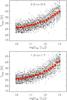 |
Fig. 3 Simulations revealing the effects of stacking on our dust temperature estimates. Empty black circles represent our 1000 simulated galaxies following the Tdust − LIR correlation of Chapman et al. (2003). Large filled orange circles represent the mean dust temperature of galaxies in a given infrared luminosity bin. Large filled red stars represent the dust temperature inferred from the mean PACS/SPIRE flux densities of galaxies in a given infrared luminosity bin. The Chapman et al. (2003) derivation of the median and interquartile range of the Tdust − LIR relation observed at z ~ 0 is shown by solid and dash-dotted lines, linearly extrapolated to 1013 L⊙. In the top panel, simulated galaxies are in the 0.2 < z < 0.5 redshift bin, while in the bottom panel simulated galaxies are in the 1.2 < z < 1.7 redshift bin. |
We find that the mean dust temperatures and those inferred from the mean FIR SEDs only differ by a few degrees. Moreover, we do not find any strong systematic biases as a function of either LIR or redshift, and therefore conclude that the dust temperatures inferred from the stacked mean FIR SEDs accurately represent the underlying galaxy population. We note that a flattening of the Tdust − LIR correlation with redshift as found in Symeonidis et al. (2013) does not change our results, as they do not strongly depend on the slope of the Tdust − LIR correlation but rather on its dispersion.
4. Results
4.1. The SFR–M∗–z parameter space
We have seen in Sect. 2.7 that incompleteness in our initial sample should not affect our ability to study variations of Tdust in the SFR− M∗ plane. However, one additional source of incompleteness might still affect our study: our ability to derive accurate Tdust for each SFR–M∗ − z bin. Therefore, before presenting the variations of dust temperature in the SFR− M∗ plane, we examine which regions of the SFR–M∗ − z parameter space have accurate Tdust estimates from individual detections, and from our stacking analysis. The left panel of Fig. 4 presents the fraction of sources (i.e., the completeness) in a given SFR–M∗ − z bin with individual FIR detections and accurate dust temperature estimates (see Sect. 3.1). The right panel of Fig. 4 presents the same quantity for the stacking analysis. There, each SFR− M∗ − z bin corresponds to only one set of stacked FIR flux densities and thus one dust temperature estimate. Consequently, in the right panel of Fig. 4, the completeness can only take two different values: 0% if the dust temperature estimate is inaccurate; 100% if the dust temperature estimate is accurate.
For galaxies individually detected in our PACS/SPIRE images reliable dust temperatures are only obtained in SFR− M∗ bins situated above a given SFR threshold. This SFR threshold increases with redshift and translates into a threshold in LIR. If keeping above this threshold, the Tdust − LIR relation can therefore be studied without biases. However, because the region of the SFR–M∗ plane with high completeness in all redshift bins is relatively small, we conclude that the PACS/SPIRE detections are not sufficient to draw strong conclusions on the redshift evolution of the Tdust − LIR relation. The prognostic for using the PACS/SPIRE detections to study the Tdust − Δlog (SSFR)MS and Tdust − SSFR relations is even worse. Indeed, in all but our first redshift bin, the dust temperature of MS galaxies is only constrained for those with very high stellar masses. The stacking analysis is therefore required.
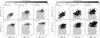 |
Fig. 4 Left: fraction of sources (i.e., completeness) in a given SFR–M∗ bin with individual PACS/SPIRE detections and accurate dust temperature estimates. Right: SFR–M∗ bins with accurate dust temperature estimates (i.e., completeness =100%), as inferred from our stacking analysis. Because each SFR–M∗ bin corresponds to only one set of stacked FIR flux densities and thus one dust temperature estimate, here the completeness can only take two different values: 0% if the dust temperature estimate is inaccurate; 100% if the dust temperature estimate is accurate. The quality of our dust temperature estimates were evaluated using criteria presented in Sects. 3.1 and 3.2. Short-dashed lines on a white background show the MS of star formation. |
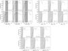 |
Fig. 5 Fraction of SFR− M∗ bins with M∗ > 1010 M⊙ and with accurate dust temperature estimates (see Sect. 3.1) in our stacking analysis as function of their Δlog (SSFR)MS (top left panel), LIR (top right panel) or SSFR (bottom panel). Horizontal dashed lines represent the 80% completeness limits. Hatched areas represent the regions of parameter space affected by incompleteness, i.e., where less than 80% of our SFR− M∗ bins have accurate dust temperature estimates. Shaded regions in the top left panel show the location and dispersion of the MS of star formation. |
The right panel of Fig. 4 illustrates the regions of
the SFR–M∗ − z parameter space reachable with
our stacking analysis. The SFR completeness limit of the stacking analysis depends on the
stellar masses: it is nearly constant at intermediate stellar masses, but increases at
both very high and low stellar masses. These variations are caused by changes in the
number of galaxies in the SFR− M∗ bins. At fixed SFR, the
SFR− M∗ bins with low stellar masses are located above the
MS and thus contain far fewer sources than those with intermediate stellar masses and
which probe the bulk of the MS. Similarly, at fixed SFR,
SFR− M∗ bins with very high stellar masses are located below
the MS of star formation and thus contain far fewer sources than those with intermediate
stellar masses and which probe the MS of star formation. The decrease in the number of
sources in these SFR− M∗ bins naturally translates into higher
SFR completeness limits in our stacking analysis ( ). Due to the very strong increase in the
SFR completeness limits at low stellar masses, we restrict our study to galaxies with
M∗ > 1010 M⊙.
). Due to the very strong increase in the
SFR completeness limits at low stellar masses, we restrict our study to galaxies with
M∗ > 1010 M⊙.
Figure 5 illustrates our ability to study the variations of Tdust in the SFR–M∗ plane for galaxies with M∗ > 1010 M⊙ through the stacking analysis. In these figures we show the fraction of SFR− M∗ bins with reliable dust temperature estimates (see Sect. 3.1) as a function of their Δlog (SSFR)MS, LIR and SSFR. In the rest of the paper, we consider that the mean dust temperature in a given Δlog (SSFR)MS, LIR or SSFR bin is fully constrained if and only if the completeness in this bin is at least 80%.
In each redshift bin, our stacking analysis allows us to fully constrain the mean dust temperature of galaxies situated on and above the MS of star formation at such a completeness level, and therefore to reliably study the redshift evolution of the Tdust − Δlog (SSFR)MS correlation. The stacking analysis furthermore allows us to constrain the mean dust temperature of galaxies over more than an order of magnitude in LIR and SSFR. However, because our LIR and SSFR completeness limits increase with redshift, the LIR and SSFR ranges probed in our different redshift bins do not fully overlap. Thus while we can robustly constrain the Tdust − LIR and Tdust–SSFR correlations in all our redshift bins, the study of their evolution with redshift is somewhat limited.
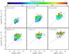 |
Fig. 6 Mean dust temperature of galaxies in the SFR− M∗ plane as found from individual detections. Short-dashed lines on a white background show the MS of star formation. Solid contours indicate the regions in which at least 50% of the galaxies have accurate dust temperature estimates. Outside these regions results have to be treated with caution, because they are inferred from incomplete samples. Tracks of iso-dust-temperature are not characterised by vertical or horizontal lines but instead by approximately diagonal lines. |
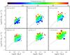 |
Fig. 7 Mean dust temperature of galaxies in the SFR− M∗ plane as found from our stacking analysis. Short-dashed lines on a white background show the MS of star formation. Tracks of iso-dust-temperature are not characterised by vertical or horizontal lines but instead by approximately diagonal lines. |
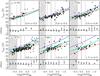 |
Fig. 8 Dust temperature of galaxies as a function of Δlog (SSFR)MS, as derived from our stacking analysis. Empty circles show results for SFR–M∗ bins with low stellar masses, i.e., M∗ < 1010.5, 1010.7, 1010.7, 1010.8, 1010.8 and 1010.9 M⊙ in our 0 < z < 0.2, 0.2 < z < 0.5, 0.5 < z < 0.8, 0.8 < z < 1.2, 1.2 < z < 1.7 and 1.7 < z < 2.3 bins, respectively. Filled circles show results for SFR–M∗ bins with high stellar masses. In each panel, we give the Spearman correlation factor derived from our data points. Dashed red lines correspond to a linear fit to the data points of the 0.2 < z < 0.5 redshift bin. Triple-dot-dashed green lines represent predictions inferred from the variations of the SFE with Δlog (SSFR)MS and variations of the metallicity with redshift (see Eqs. (10) and (11)). Long-dashed light blue lines represent predictions inferred from the variations of the SFE with Δlog (SSFR)MS and variations of the normalisation of the SFE-Δlog (SSFR)MS relation with redshift (see Eqs. (10) and (13)). Dot-dashed dark blue lines represent predictions inferred from the variations of the SFE with Δlog (SSFR)MS, and variations with redshift of the normalisation of the SFE–Δlog (SSFR)MS relation and of the metallicity (see Eqs. (10) and (14)). Hatched areas represented the regions of parameter space affected by incompleteness (see text and Fig. 5). Vertical solid and dot-dashed lines show the localisation and width of the MS of star formation. The lower panel of each redshift bin shows the offset between the median dust temperature of our data points and the red dashed line, in bins of 0.2 dex. |
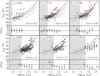 |
Fig. 9 Dust temperature of galaxies as a function of LIR, as derived from our stacking analysis. In each panel, we give the Spearman correlation factor derived from our data points. Red dashed lines correspond to a second order polynomial fit to the data points of the 0.2 < z < 0.5 redshift bin. Hatched areas represented the regions of parameter space affected by incompleteness (see text and Fig. 5). The Chapman et al. (2003) derivation of the median and interquartile range of the relation observed at z ~ 0 is shown by solid and dot-dashed lines, linearly extrapolated to 1013 L⊙. The lower panel of each redshift bin shows the offset between the median dust temperature of our data points and the dashed red line, in bins of 0.3 dex. |
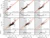 |
Fig. 10 Dust temperature of galaxies as a function of SSFR, as derived from our stacking analysis. In each panel, we give the Spearman correlation factor derived from our data points. Dashed red lines correspond to a linear fit to the data points of the 0.2 < z < 0.5 redshift bin. Dot-dashed orange lines show the redshift evolution of the Tdust–SSFR relation, fixing its slope to that observed in the 0.2 < z < 0.5 redshift bin (i.e., slope of the dashed red line) and fitting its zero point with a A × (1 + z)B function (see Eq. (5)). Hatched areas represent the regions of parameter space affected by incompleteness (see text and Fig. 5). The lower panel of each redshift bin shows the offset between the median dust temperature of our data points and the dashed red line, in bins of 0.3 dex. |
4.2. Dust temperature in the SFR–M∗–z parameter space
Figures 6 and 7 show the mean dust temperatures of galaxies in our SFR–M∗ − z bins as inferred using individual detections and our stacking analysis, respectively. In these figures, we only used accurate dust temperature estimates (see Sect. 3.1). For the detections, the black contours indicate regions where at least 50% of the galaxies in a given SFR− M∗ bin have reliable dust temperature estimates. Outside these regions, results have to be treated with caution, because they rely on very incomplete samples. Both figures clearly show that in any given redshift bin, Tdust does not evolve simply with their SFR or with their stellar mass, but instead with a combination of these two parameters. In other words, tracks of iso-dust temperature are not characterised by vertical or horizontal lines, but instead by diagonal lines.
To investigate which parameter best correlates with the dust temperature of galaxies, we show in Figs. 8–10 the variation of the dust temperature of galaxies as function of their Δlog (SSFR)MS, LIR and SSFR, respectively. Because individual detections do not probe large ranges in the Δlog (SSFR)MS, LIR and SSFR parameter spaces, here we only rely on dust temperatures inferred from our stacking analysis. In these figures, the dashed regions indicate regimes of parameter space affected by large incompleteness as defined in Fig. 5. Constraints in these regions have to be treated with caution.
In each redshift interval, the dust temperature of galaxies better correlates with their Δlog (SSFR)MS and SSFR values than with LIR, as revealed by the Spearman correlation factors of the relations between Tdust and these three quantities. The Spearman correlation factors of the Tdust − Δlog (SSFR)MS and Tdust–SSFR correlations are statically equivalent in all our redshift bins. From this analysis we can conclude that the dust temperature of galaxies is more fundamentally linked to their SSFR and Δlog (SSFR)MS than to their LIR.
To go further in our understanding of the Tdust − LIR, Tdust − Δlog (SSFR)MS and Tdust–SSFR correlations, we also study their redshift evolution. We first fit the Tdust − LIR, Tdust − Δlog (SSFR)MS and the Tdust–SSFR correlations in the 0.2 < z < 0.5 redshift bin, where for all three correlations the Spearman correlation factor is highest, and the region of parameter space reliably probed is largest. The Tdust − LIR correlation is fitted with a second order polynomial function, while the Tdust − Δlog (SSFR)MS and the Tdust–SSFR correlations are fitted with linear functions. We note that Chapman et al. (2003) described the Tdust − LIR correlation using a double power-law function instead of a second order polynomial. However, this specific choice does not affect our results.
Once these best-fitting relations are established in the most reliable redshift interval, the fits are compared with the other intervals to track the redshift evolution of the normalisation of these relations. The Tdust − Δlog (SSFR)MS correlation seems to smoothly evolve from z = 0 to z = 2.3, with dust temperatures increasing with redshift at fixed Δlog (SSFR)MS. Similarly, the Tdust–SSFR correlation smoothly evolves up to z ~ 2, with the dust temperature of galaxies evolves towards colder values at high redshift at fixed SSFR. Finally, the Tdust − LIR correlation slightly evolves from z = 0 to z = 2.3, with high redshift galaxies exhibiting colder dust temperatures than their low redshift counterparts. We note that the Tdust − LIR correlations found here are consistent with those of Symeonidis et al. (2013) which are based on individual detections.
To reproduce the redshift evolution of the
Tdust − Δlog (SSFR)MS and
Tdust–SSFR relations, we fixed their slopes
to those measured in the 0.2 < z < 0.5 redshift bin and fitted
their zero points using an
A × (1 + z)B function.
For the Tdust − Δlog (SSFR)MS
relation, we find  (4)while for the
Tdust–SSFR relation we find
(4)while for the
Tdust–SSFR relation we find  (5)Because the
Tdust − Δlog (SSFR)MS and
Tdust–SSFR correlations are statistically
very significant, they supersede the
Tdust − LIR correlation
classically used to predict the dust temperature of galaxies. In particular, Eq. (5), which only relies on the stellar masses,
SFRs and redshifts of galaxies, could be used to improve FIR predictions from
semi-analytical or backward evolutionary models.
(5)Because the
Tdust − Δlog (SSFR)MS and
Tdust–SSFR correlations are statistically
very significant, they supersede the
Tdust − LIR correlation
classically used to predict the dust temperature of galaxies. In particular, Eq. (5), which only relies on the stellar masses,
SFRs and redshifts of galaxies, could be used to improve FIR predictions from
semi-analytical or backward evolutionary models.
5. Discussion
Using deep Herschel observations and a careful stacking analysis, we found, over a broad range of redshift, that the dust temperature of galaxies better correlates with their SSFRs or their Δlog (SSFR)MS values than with LIR. This finding supersedes the Tdust − LIR correlation classically implemented in FIR SED template libraries. These results also provide us with important information on the conditions prevailing in the star-forming regions of galaxies and the evolution of these conditions as a function of redshift.
5.1. Tdust variations in the SFR–M∗ plane at fixed redshift
In a given redshift bin, our results unambiguously reveal that the dust temperature of galaxies correlates with their SSFR or equivalently with their Δlog (SSFR)MS (at a given redshift, SSFR and Δlog (SSFR)MS are nearly equivalent because the slope of the MS is close to unity; log(SFRMS) = log ( M∗) + C(z), so log [SSFRMS(M∗,z)] = C(z) and Δlog (SSFR)MS = log [SSFR(galaxy)] − C(z). The universality of the dust temperature at fixed Δlog (SSFR)MS indicates that galaxies with a given Δlog (SSFR)MS are composed of the same type of star-forming regions and that the increase in SFR with stellar mass is only due to an increase in the number of such star-forming regions. In that picture, galaxies situated on the MS are dominated by star-forming regions with relatively low radiation fields and thus relatively cold dust temperatures, while galaxies situated far above the MS are dominated by star-forming regions exposed to extremely high radiation fields, yielding hotter dust temperatures.
As a first approximation, and in the case where star-forming regions are optically thick
in the rest-frame UV and optically thin in the rest-frame FIR, one can link the dust
temperature of a galaxy to the radiation field seen per unit of dust mass: 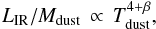 (6)i.e., the dust temperature of a galaxy
increases if the input radiation is delivered to fewer dust grains. In that approximation,
one can then link the dust temperature of galaxies to the radiation field seen per unit of
gas mass (i.e., LIR/Mgas), via the
gas-to-dust ratio relation:
(6)i.e., the dust temperature of a galaxy
increases if the input radiation is delivered to fewer dust grains. In that approximation,
one can then link the dust temperature of galaxies to the radiation field seen per unit of
gas mass (i.e., LIR/Mgas), via the
gas-to-dust ratio relation:  (7)where μ is the metallicity
(Leroy et al. 2011). At fixed stellar mass
(equivalent to fixed metallicity, assuming a mass-metallicity relation), the smooth
increase in dust temperature with Δlog (SSFR)MS could thus
be interpreted as an increase in
LIR/Mgas, i.e., the
star-formation efficiency (SFE) of galaxies. Using direct molecular gas observations,
several studies have effectively observed a significant increase in the SFE with
Δlog (SSFR)MS (Saintonge
et al. 2011a,b, 2012; Genzel et al. 2010; Daddi et al. 2010). In their local Universe sample,
Saintonge et al. (2012) found
(7)where μ is the metallicity
(Leroy et al. 2011). At fixed stellar mass
(equivalent to fixed metallicity, assuming a mass-metallicity relation), the smooth
increase in dust temperature with Δlog (SSFR)MS could thus
be interpreted as an increase in
LIR/Mgas, i.e., the
star-formation efficiency (SFE) of galaxies. Using direct molecular gas observations,
several studies have effectively observed a significant increase in the SFE with
Δlog (SSFR)MS (Saintonge
et al. 2011a,b, 2012; Genzel et al. 2010; Daddi et al. 2010). In their local Universe sample,
Saintonge et al. (2012) found  (8)for
− 0.5 < Δlog (SSFR)MS < 1. Combining Eqs. (6)–(8), assuming that Δlog (SSFR)MS and
μ are independent, and assuming that the gas-to-dust relation of Leroy et al. (2011) holds at high redshift, we can thus
predict from the gas phase the evolution of the dust temperature as a function of
Δlog (SSFR)MS and μ:
(8)for
− 0.5 < Δlog (SSFR)MS < 1. Combining Eqs. (6)–(8), assuming that Δlog (SSFR)MS and
μ are independent, and assuming that the gas-to-dust relation of Leroy et al. (2011) holds at high redshift, we can thus
predict from the gas phase the evolution of the dust temperature as a function of
Δlog (SSFR)MS and μ: 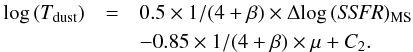 (9)Over the range of stellar masses probed by
our sample (i.e., ~1.5 dex), we expect, based on the mass-metallicity relation, an
increase in metallicity of ~0.25 dex (~0.4 dex) at z = 0
(z = 2) (Tremonti et al. 2004;
z = 2, Erb et al. 2006; see also
Genzel et al. 2012). At fixed
Δlog (SSFR)MS, the dust temperatures of galaxies with
high stellar masses should thus be lower by a factor 1.09 (1.15) than those of galaxies
with low stellar masses (see Eq. (9) and
assuming β = 1.5). On the MS, this corresponds to a dust temperature
variation of ~2 K (5 K). Differentiating galaxies by stellar masses in Fig. 8 supports this prediction. As a consequence, we can
assume that:
(9)Over the range of stellar masses probed by
our sample (i.e., ~1.5 dex), we expect, based on the mass-metallicity relation, an
increase in metallicity of ~0.25 dex (~0.4 dex) at z = 0
(z = 2) (Tremonti et al. 2004;
z = 2, Erb et al. 2006; see also
Genzel et al. 2012). At fixed
Δlog (SSFR)MS, the dust temperatures of galaxies with
high stellar masses should thus be lower by a factor 1.09 (1.15) than those of galaxies
with low stellar masses (see Eq. (9) and
assuming β = 1.5). On the MS, this corresponds to a dust temperature
variation of ~2 K (5 K). Differentiating galaxies by stellar masses in Fig. 8 supports this prediction. As a consequence, we can
assume that:  (10)with variations in metallicities
(equivalently M∗) creating a dispersion of a few degrees
around this relation. In Fig. 8, we compare the
prediction from Eq. (10), assuming
β = 1.5, with the observed
Tdust − Δlog (SSFR)MS
relations. There is a very good agreement between the slope of our predictions and the
observations. We conclude that variations in dust temperature with
Δlog (SSFR)MS can be, qualitatively and quantitatively,
explained by the variation of the SFE with Δlog (SSFR)MS,
as observed by Saintonge et al. (2012). We note
that the smooth evolution of the dust temperature (equivalently SFE) with
Δlog (SSFR)MS could correspond to a smooth evolution of
the ISM conditions with Δlog (SSFR)MS, or to a linear
combination of two types of star-forming regions, i.e.: (i) cold star-forming regions
formed in secularly evolving galaxies; and (ii) hot star-forming regions formed in
starbursting galaxies via large gravitational instabilities (e.g., major mergers).
Unfortunately, using our unresolved observations we cannot discriminate between these two
interpretations.
(10)with variations in metallicities
(equivalently M∗) creating a dispersion of a few degrees
around this relation. In Fig. 8, we compare the
prediction from Eq. (10), assuming
β = 1.5, with the observed
Tdust − Δlog (SSFR)MS
relations. There is a very good agreement between the slope of our predictions and the
observations. We conclude that variations in dust temperature with
Δlog (SSFR)MS can be, qualitatively and quantitatively,
explained by the variation of the SFE with Δlog (SSFR)MS,
as observed by Saintonge et al. (2012). We note
that the smooth evolution of the dust temperature (equivalently SFE) with
Δlog (SSFR)MS could correspond to a smooth evolution of
the ISM conditions with Δlog (SSFR)MS, or to a linear
combination of two types of star-forming regions, i.e.: (i) cold star-forming regions
formed in secularly evolving galaxies; and (ii) hot star-forming regions formed in
starbursting galaxies via large gravitational instabilities (e.g., major mergers).
Unfortunately, using our unresolved observations we cannot discriminate between these two
interpretations.
We note that Magdis et al. (2012) report no dust temperature variations between galaxies situated on the lower and upper part of the MS (i.e., − 0.4 < Δlog (SSFR)MS < 0.4). Based on this finding, they argue that across the MS, the main parameter controlling Δlog (SSFR)MS is fgas ≡ Mgas/M∗ (i.e., SFE being roughly constant): at fixed stellar mass, galaxies situated on the lower part of the MS would contain less molecular gas (i.e., have lower fgas) than galaxies situated on the upper part of the MS. While Saintonge et al. (2012) qualitatively confirmed the increase in fgas across the MS, they also found a significant increase in SFE which leads to the increase in Tdust across the MS found in our sample. Thus, our results, as well as those of Saintonge et al. (2012), support the hypothesis that the localisation of a galaxy across the MS is not only controlled by fgas but rather by both SFE and fgas.
5.2. Tdust variations in the SFR−M∗ plane as function of the redshift
While the slope of the Tdust − Δlog (SSFR)MS correlation is the same in all our redshift bins, its normalisation evolves towards hotter dust temperatures at higher redshift. In our simple description, the dust temperature of a galaxy only depends on its SFE and metallicity; therefore one should also observe variations of these parameters with redshift.
In the stellar mass range of our study (i.e.,
1010 M⊙ < M∗ < 1011.5),
the metallicity μ of galaxies systematically decreases by ~0.5 dex
from z = 0 to z = 2 (z = 0, Tremonti et
al. 2004; z = 2, Erb et al. 2006; Shapley et al. 2005; Liu et al. 2008; Zahid et al. 2013; see also Genzel et al. 2012). At fixed Δlog (SSFR)MS and
assuming β = 1.5, this decrease in the metallicity should translate into
an increase in the dust temperature by a factor ~1.2. For MS galaxies, this
corresponds to a rise from 26 K to 31 K between z = 0 to
z = 2 (see Eq. (9)).
More generally, on the MS we can predict: ![Mathematical equation: \begin{equation} \label{eq:Tdust MS} {\rm log(}T_{\rm dust}^{\rm MS}[z])=-0.85\times1/(4+\beta)\times\Delta\mu[z]+C_4, \end{equation}](/articles/aa/full_html/2014/01/aa22217-13/aa22217-13-eq213.png) (11)where
Δμ [z] = − 1.05 × log(1+z)
describes the mean increase in the metallicity with redshift over the stellar mass range
probed by our sample. This formula is used to normalise the predicted
Tdust − Δlog (SSFR)MS
correlation, assuming
(11)where
Δμ [z] = − 1.05 × log(1+z)
describes the mean increase in the metallicity with redshift over the stellar mass range
probed by our sample. This formula is used to normalise the predicted
Tdust − Δlog (SSFR)MS
correlation, assuming ![Mathematical equation: \hbox{$T_{\rm dust}^{\rm MS}[z=0]=26\,$}](/articles/aa/full_html/2014/01/aa22217-13/aa22217-13-eq215.png) K and β = 1.5 (see Fig.
8). Our predictions are perfectly in line with the
observations. We thus conclude that the evolution of metallicity with redshift might be
the main driver of the normalisation of the
Tdust − Δlog (SSFR)MS
correlation. We note that in the local Universe an evolution of the dust temperature with
metallicity has already been observed (Engelbracht et al.
2008). In that study the slope of the
Tdust–metallicity relation roughly follows our predictions,
i.e.,
log (Tdust) = − 0.85 × 1/(4 + β) × μ + C4.
K and β = 1.5 (see Fig.
8). Our predictions are perfectly in line with the
observations. We thus conclude that the evolution of metallicity with redshift might be
the main driver of the normalisation of the
Tdust − Δlog (SSFR)MS
correlation. We note that in the local Universe an evolution of the dust temperature with
metallicity has already been observed (Engelbracht et al.
2008). In that study the slope of the
Tdust–metallicity relation roughly follows our predictions,
i.e.,
log (Tdust) = − 0.85 × 1/(4 + β) × μ + C4.
Tacconi et al. (2013) found that the SFE of MS
galaxies evolves from z = 0 to z = 1.5 following:
 (12)This increase in the SFE should translate
into an increase in the dust temperature by a factor ~1.2 between
z = 0 to z = 2, i.e., for MS galaxies rising from 26 K
to 31 K. More generally, on the MS we can predict:
(12)This increase in the SFE should translate
into an increase in the dust temperature by a factor ~1.2 between
z = 0 to z = 2, i.e., for MS galaxies rising from 26 K
to 31 K. More generally, on the MS we can predict: ![Mathematical equation: \begin{equation} \label{eq:Tdust MS renor} {\rm log\,(}T_{\rm dust}^{\rm MS}[z])=1/(4+\beta)\times{\rm log}\,(1+z)+C_6, \end{equation}](/articles/aa/full_html/2014/01/aa22217-13/aa22217-13-eq219.png) (13)This formula is also used to normalise the
predicted Tdust − Δlog (SSFR)MS
correlation, assuming K and β = 1.5 (see Fig.
8). Because these predictions are also in line with
our observations, we conclude that the evolution of the SFE with redshift might also be
the main driver of the normalisation of the
Tdust − Δlog (SSFR)MS
correlation.
(13)This formula is also used to normalise the
predicted Tdust − Δlog (SSFR)MS
correlation, assuming K and β = 1.5 (see Fig.
8). Because these predictions are also in line with
our observations, we conclude that the evolution of the SFE with redshift might also be
the main driver of the normalisation of the
Tdust − Δlog (SSFR)MS
correlation.
Combining the evolution of both the SFE and metallicity with redshift, we can predict,
![Mathematical equation: \begin{equation} \label{eq:Tdust MS tot} {\rm log(}T_{\rm dust}^{\rm MS}[z])=(0.85\times1.05+1)/(4+\beta)\times{\rm log}(1+z)+C_7, \end{equation}](/articles/aa/full_html/2014/01/aa22217-13/aa22217-13-eq220.png) (14)In Fig. 8, we present the predictions from this formula, assuming
K and β = 1.5. We observe
that it overestimates the normalisation with redshift of the
Tdust − Δlog (SSFR)MS
correlation.
(14)In Fig. 8, we present the predictions from this formula, assuming
K and β = 1.5. We observe
that it overestimates the normalisation with redshift of the
Tdust − Δlog (SSFR)MS
correlation.
In a simple optically thin model where Tdust directly traces the galaxy-integrated LIR and Mdust, our findings can be summarised as follows:
-
At fixed redshift, the main parameter controlling the variation of Tdust with Δlog (SSFR)MS is the SFE of galaxies: galaxies with high Δlog (SSFR)MS are more efficient in turning their gas into stars, which leads to higher input power per unit of dust mass and therefore higher dust temperatures.
-
At fixed Δlog (SSFR)MS, the increase in the metallicity with the stellar masses can explain some of the scatter observed in the Tdust − Δlog (SSFR)MS and Tdust − SSFR correlations.
-
The normalisation with redshift of the Tdust − Δlog (SSFR)MS correlation towards hotter dust temperatures can be explained by the global decrease in the metallicity of galaxies with redshift or by the global increase in the SFE of galaxies with redshift. However, combining the evolution of both the metallicity and SFE with redshift, we overestimate the normalisation towards hotter dust temperatures of the Tdust − Δlog (SSFR)MS correlation. This may indicate that the assumptions of our simple model do not hold. In particular, the scaling relations that we adopted for the evolution of the metallicity and SFE with redshift and with offset from the MS might be overall inconsistent. This will need future revision.
Finally, we note that Nordon et al. (2012) and Elbaz et al. (2011) found the PAH-to-LIR ratio, parametrized as L8/LIR, to strongly correlate with Δlog (SSFR)MS. This correlation appears to remain the same up to zs2. Therefore, PAHs and dust temperatures do not evolve in the same manner as a function of redshift. This situation could arise from differences in the mechanics heating the PAHs and the dust components dominating the FIR emission of galaxies. In the model of Draine & Li (2007), the fraction of power radiated into the 7.9 μm band by the single-photon heated PAHs, observed as L8/LIR, is essentially proportional to qPAH, the fraction of dust mass in the form of PAH grains with less than 103 carbon atoms. It does not appear to scale with ⟨ U ⟩, the mean intensity seen per unit of dust mass (see Figs. 19c and d of Draine & Li 2007). Consequently, in this model, a strong increase in the dust temperature can occur while the PAH-to-LIR ratio remains constant, if qPAH remains the same and the intensity of the radiation field seen by the dust increases. The question is thus: at fixed Δlog (SSFR)MS, is qPAH affected by the evolution of the metallicity with redshift or by the evolution of the SFE with redshift? In local star-forming galaxies and in the metallicity range of our sample (μ > 8.1), there is only a weak correlation between the metallicity and the PAH-to-LIR ratio (Smith et al. 2007; Engelbracht et al. 2008; Hunt et al. 2010). Thus, the evolution of the metallicity with redshift might affect the normalisation of the Tdust − Δlog (SSFR)MS correlation but not significantly affect qPAH and thus leads to the universal (PAH-to-LIR)–Δlog (SSFR)MS correlation observed in Elbaz et al. (2011) and Nordon et al. (2012). For the SFE, the situation is somewhat different. At fixed redshift, we have explained the Tdust − Δlog (SSFR)MS correlation using the SFE–Δlog (SSFR)MS correlation observed by Saintonge et al. (2012). Following a similar train of thought, one could thus also ascribe the (PAH-to-LIR) – Δlog (SSFR)MS correlation to the SFE–Δlog (SSFR)MS correlation. In this case, however, one would expect to observe an evolution with redshift of the normalisation of both the Tdust − Δlog (SSFR)MS and (PAH-to-LIR)–Δlog (SSFR)MS correlations, following the evolution with redshift of the normalisation of the SFE–Δlog (SSFR)MS correlation. Is the universality of the (PAH-to-LIR)–Δlog (SSFR)MS correlation to be interpreted as a proof that actually the SFE–Δlog (SSFR)MS correlation does not significantly evolve with redshift? And that the evolution of the metallicity with redshift is the main driver for the normalisation of the Tdust − Δlog (SSFR)MS correlation? To obtain answers to these questions, additional studies are required.
5.3. Towards a better understanding of the MS of star formation
The existence of the MS of star formation is currently interpreted as evidence that the bulk of the galaxy population is forming stars gradually with long duty cycles. In this picture, MS galaxies evolve with a secular mode of star formation, likely sustained by a continuous gas accretion from the IGM and along the cosmic web (Dekel et al. 2009; Davé et al. 2010), while star-forming galaxies located far above the MS evolve through strong starbursts with short duty-cycles, mainly triggered by major mergers. The strong correlation observed between Tdust and Δlog (SSFR)MS gives weight to this interpretation. It unambiguously reveals that the physical conditions prevailing in the star-forming regions of on- and far-above-MS galaxies are not the same. Furthermore, because the Tdust − Δlog (SSFR)MS correlation can be understood as a variation of the SFE with Δlog (SSFR)MS, it also supports the hypothesis of different modes of star formation for these two populations of galaxies. Unfortunately, using our unresolved observations we cannot distinguish if galaxies lying at intermediate distance from the MS correspond to a linear combination or to a smooth evolution of the ISM conditions between these two extreme cases.
In line with our findings, Magnelli et al. (2012b) found that on- and above-MS galaxies exhibit different CO-to-H2 conversion factors (i.e., αCO), indicating differences in the physical conditions prevailing in their giant molecular clouds (GMCs, Genzel et al. 2010; Daddi et al. 2010). MS galaxies have high αCO factors, consistent with star-forming regions mainly composed of well virialized GMCs, while above-MS galaxies have low αCO factors consistent with star-forming regions being mainly unvirialized GMCs as observed in local major mergers. Combined with other independent observational properties, the current vision of the main-sequence of star formation can be summarised as follows. Galaxies situated on the MS of star formation have disk-like morphology (Wuyts et al. 2011b), have star-forming regions mainly composed of virialized GMCs (Magnelli et al. 2012b), have relatively low SFR surface density (Wuyts et al. 2011b), high PAH-to-LIR ratio (Elbaz et al. 2011; Nordon et al. 2012), high C ii-to-LIR ratio (Graciá-Carpio et al. 2011) and cold dust temperature. Galaxies situated far above the MS have bulge-like morphology, star-forming regions dominated by unvirialized GMCs, have relatively high SFR surface density, low PAH-to-LIR ratio, low C ii-to-LIR and hot dust temperature. All these independent observations give strong weight to the interpretation where on- and above-MS galaxies evolve through different modes of star formation, a secular and a starbursting mode, respectively.
6. Summary
Using deep Herschel PACS and SPIRE observations of the GOODS-N, GOODS-S and COSMOS fields, we study variations of the dust temperature of galaxies in the SFR− M∗ plane up to zs2. Dust temperatures are inferred using the stacked PACS/SPIRE FIR photometries of each SFR–M∗ − z bin. Based on this careful analysis, we constrain the dust temperature of galaxies over a broad range of redshifts, and study the evolution of the Tdust − LIR, Tdust − SSFR and Tdust − Δlog (SSFR)MS correlations. Then, using a simple model linking the dust temperature with the dust and gas contents of the ISM, we discuss these correlations in terms of variations of the physical conditions prevailing in the star-forming regions of galaxies. Our main conclusions are:
-
1.
Over a broad range of redshifts, the dust temperature of galaxiessmoothly increases with their infrared luminosities, SSFRs and Δlog (SSFR)MSvalues. The Tdust − SSFR and Tdust − Δlog (SSFR)MS correlations are statistically much moresignificant than the Tdust − LIR correlation. The slope of the Tdust − Δlog (SSFR)MS correlation doesnot evolve up to z s 2, but its normalisation does: at a given Δlog (SSFR)MS,high-redshift galaxies exhibit hotter dust temperatures than theirlocal counterparts. Similarly, the normalisation of the Tdust–SSFRcorrelation evolves towards colder dust temperatures up to z ~ 2. The Tdust − LIRcorrelation also evolves with redshift: at fixed LIR, high-redshiftgalaxies exhibit slightly colder dust temperatures than their localcounterparts.
-
2.
Because the Tdust − Δlog (SSFR)MS and Tdust–SSFR correlations are statistically very significant, they supersede the Tdust − LIR correlation classically used to predict the dust temperatures of galaxies. These correlations could be used to improve results of semi-analytical or backward evolutionary models.
-
3.
In a simple optically thin model, where Tdust directly traces the galaxy-integrated LIR and Mdust, the slope of the Tdust − Δlog (SSFR)MS (equivalently SSFR at fixed z) correlation can be explained, qualitatively and quantitatively, by the increase in the SFE with Δlog (SSFR)MS found locally by molecular gas studies (Saintonge et al. 2012). In addition, the normalisation with redshift of the Tdust − Δlog (SSFR)MS correlation can be explained by the global decrease in the metallicity of galaxies with redshift (Tremonti et al. 2004; Erb et al. 2006) or by the increase in the SFE of MS galaxies with redshift (Tacconi et al. 2013). However, combining the evolution of both the metallicity and SFE with redshift, we overestimate the normalisation towards hotter dust temperatures of the Tdust − Δlog (SSFR)MS correlation. This may indicate that the assumptions of our simple model do not hold. In particular, the scaling relations that we adopted for the evolution of the metallicity and SFE with redshift and with offset from the MS might be overall inconsistent. This will need future revision.
All these results support the hypothesis that the conditions prevailing in the star-forming regions of MS and far-from-MS galaxies are different. MS galaxies have star-forming regions with low SFEs and thus cold dust temperatures, while galaxies situated far above the MS seems to be in a starbursting phase characterised by star-forming regions with high SFEs and thus hot dust temperatures. Galaxies lying at intermediate distance from the MS could correspond, for our unresolved observations, to a linear combination or to a smooth evolution of the physical conditions between these two extreme star-forming regions. In that picture, at fixed Δlog (SSFR)MS, galaxies are dominated by the same type of star-forming regions and the increase in SFR with M∗ is due to an increase in the number of such star-forming regions.
Online material
Appendix A: Far-infrared SEDs
Figure A.1 presents the FIR properties of some of our galaxies with individual FIR detections. In the first column, galaxies were randomly selected within a sample with 1010.8 < M∗ [M⊙] < 1011 and − 0.1 < Δlog (SSFR)MS < 0.1. In the second column, galaxies were randomly selected within a sample with 1010.8 < M∗ [M⊙] < 1011 and Δlog (SSFR)MS > MAX [Δlog (SSFR)MS] − 0.1. To derive the infrared luminosities and dust temperatures of these galaxies (see Sects. 2.6, 3.1 and Table A.1), we fitted their FIR flux densities with the DH SED template library.
Dust temperatures assigned to the DH SED templates by fitting their simulated z = 0 PACS/SPIRE flux densities with a single modified (i.e., β = 1.5) blackbody function.
Figure A.2 presents the mean FIR properties of some of our SFR− M∗ bins, as inferred from our stacking analysis. In the first column, SFR− M∗ bins were selected to have 1010.8 < M∗ [M⊙] < 1011 and − 0.1 < Δlog (SSFR)MS < 0.1, while in the second column, SFR− M∗ bins were selected to have 1010.8 < M∗ [M⊙] < 1011 and Δlog (SSFR)MS = MAX [Δlog (SSFR)MS]. To derive the mean dust temperature of these SFR–M∗ bins, we fitted their FIR flux densities with the DH SED template library (see Fig. A.2).
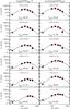 |
Fig. A.1 FIR properties of some of our galaxies with individual FIR detections. All these galaxies have 1010.8 < M∗ [M⊙] < 1011. In the first column, galaxies have − 0.1 < Δlog (SSFR)MS < 0.1 while in the second column they have Δlog (SSFR)MS > MAX [Δlog (SSFR)MS] − 0.1. Black lines show the DH SED templates best-fitting these FIR flux densities. From these fits, we inferred the infrared luminosities and dust temperatures of our galaxies. |
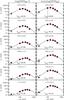 |
Fig. A.2 FIR properties of some of our SFR–M∗ bins, as inferred from our stacking analysis. These SFR–M∗ bins have 1010.8 < M∗ [M⊙] < 1011. In the first column, SFR–M∗ bins have − 0.1 < Δlog (SSFR)MS < 0.1, while in the second column they have Δlog (SSFR)MS = max [Δlog (SSFR)MS]. Black lines show the DH SED templates best-fitting these FIR flux densities. From these fits, we inferred the mean dust temperatures of galaxies in these SFR–M∗ bins. We also verified that the infrared luminosities inferred from these fits agree, within 0.3 dex, with the mean infrared luminosities inferred from our “ladder of SFR indicators” (see Sect. 2.6). |
Appendix B: The Tdust–Δlog (SSFR)MS relation in the GOODS fields
Figure B.1 presents the Tdust − Δlog (SSFR)MS relation, as inferred using the GOODS fields. Because we exclude the COSMOS observations from our stacking analysis, our ability
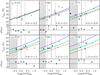 |
Fig. B.1 Dust temperature of galaxies as a function of Δlog (SSFR)MS, as derived from our stacking analysis using only the GOODS fields (i.e., excluding the COSMOS observations). Symbols and lines are the same as in Fig. 8. |
to probe and sample properly the SFR–M∗ parameter space decreases. Therefore, the number of data points available to study the Tdust − Δlog (SSFR)MS relation is significantly reduced. Despite this limitation, we still observe a Tdust − Δlog (SSFR)MS relation evolving with redshift.
Appendix C: The Tdust–Δlog (SSFR)MS relation using different definition of the MS
In this appendix we test the robustness of the Tdust − Δlog (SSFR)MS correlation against changes in the definition of the MS of star formation. Figure C.1 shows
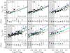 |
Fig. C.1 Dust temperature of galaxies as a function of Δlog (SSFR)MS, as derived from our stacking analysis. In this figure, the definition of the MS of star formation is taken from Elbaz et al. (2011). Symbols and lines are the same as in Fig. 8. |
the Tdust − Δlog (SSFR)MS correlation using the definition of the MS from Elbaz et al. (2011). We still observe a strong correlation between Tdust and Δlog (SSFR)MS as revealed by the high Spearman correlation factor found in all our redshift bins. Our results are thus robust against changes in the definition of the MS.
A simple IDL code implementing our results is available from the author at http://www.mpe.mpg.de/ir/Research/PEP/Tdust_sSFR. This code predicts the dust temperature and the FIR/mm flux densities of a galaxy from its SFR, M∗ and z.
Publicly available at http://www.mpe.mpg.de/ir/Research/PEP/
Although the GOODS-S and -N multi-wavelength catalogues both correspond to Ks< 24.3, the GOODS-S catalogue contains less sources than the GOODS-N catalogue because it includes sources with > 5σ while the GOODS-N multi-wavelength catalogue extends down to a 3σ significance.
Original maps from which we removed all 3σ detections.
Acknowledgments
PACS has been developed by a consortium of institutes led by MPE (Germany) and including UVIE (Austria); KU Leuven, CSL, IMEC (Belgium); CEA, LAM (France); MPIA (Germany); INAF-IFSI/OAA/OAP/OAT, LENS, SISSA (Italy); IAC (Spain). This development has been supported by funding agencies BMVIT (Austria) ESA-PRODEX (Belgium); CEA/CNES (France); DLR (Germany); ASI/INAF (Italy); and CICYT/MCYT (Spain). SPIRE has been developed by a consortium of institutes led by Cardiff University (UK) and including University of Lethbridge (Canada); NAOC (China); CEA, LAM (France); IFSI, University of Padua (Italy); IAC (Spain); Stockholm Observatory (Sweden); Imperial College London, RAL, UCL-MSSL, UKATC, University of Sussex (UK), Caltech, JPL, NHSC, University of Colorado (USA). This development has been supported by national funding agencies: CSA (Canada); NAOC (China); CEA, CNES, CNRS (France); ASI (Italy); MCINN (Spain); SNSB (Sweden); STFC, UKSA (UK); and NASA (USA). D.E. received support of the European Community Framework Programme 7, FP7-SPACE Astrodeep, grant agreement No. 312725
References
- Alexander, D. M., Bauer, F. E., Brandt, W. N., et al. 2003, AJ, 125, 383 [NASA ADS] [CrossRef] [Google Scholar]
- Baldry, I. K., Glazebrook, K., Brinkmann, J., et al. 2004, ApJ, 600, 681 [NASA ADS] [CrossRef] [Google Scholar]
- Barger, A. J., Cowie, L. L., & Wang, W.-H. 2008, ApJ, 689, 687 [NASA ADS] [CrossRef] [Google Scholar]
- Berta, S., Magnelli, B., Lutz, D., et al. 2010, A&A, 518, L30 [NASA ADS] [CrossRef] [EDP Sciences] [Google Scholar]
- Berta, S., Magnelli, B., Nordon, R., et al. 2011, A&A, 532, A49 [NASA ADS] [CrossRef] [EDP Sciences] [Google Scholar]
- Béthermin, M., Daddi, E., Magdis, G., et al. 2012a, ApJ, 757, L23 [NASA ADS] [CrossRef] [Google Scholar]
- Béthermin, M., Le Floc’h, E., Ilbert, O., et al. 2012b, A&A, 542, A58 [NASA ADS] [CrossRef] [EDP Sciences] [Google Scholar]
- Brammer, G. B., van Dokkum, P. G., & Coppi, P. 2008, ApJ, 686, 1503 [NASA ADS] [CrossRef] [Google Scholar]
- Brinchmann, J., Charlot, S., White, S. D. M., et al. 2004, MNRAS, 351, 1151 [NASA ADS] [CrossRef] [Google Scholar]
- Bruzual, G., & Charlot, S. 2003, MNRAS, 344, 1000 [NASA ADS] [CrossRef] [Google Scholar]
- Cappelluti, N., Brusa, M., Hasinger, G., et al. 2009, A&A, 497, 635 [NASA ADS] [CrossRef] [EDP Sciences] [Google Scholar]
- Chabrier, G. 2003, ApJ, 586, L133 [NASA ADS] [CrossRef] [Google Scholar]
- Chapman, S. C., Helou, G., Lewis, G. F., & Dale, D. A. 2003, ApJ, 588, 186 [NASA ADS] [CrossRef] [Google Scholar]
- Chapman, S. C., Ivison, R. J., Roseboom, I. G., et al. 2010, MNRAS, 409, L13 [NASA ADS] [CrossRef] [Google Scholar]
- Chary, R., & Elbaz, D. 2001, ApJ, 556, 562 [NASA ADS] [CrossRef] [Google Scholar]
- Cimatti, A., Cassata, P., Pozzetti, L., et al. 2008, A&A, 482, 21 [NASA ADS] [CrossRef] [EDP Sciences] [Google Scholar]
- Cohen, J. G., Hogg, D. W., Blandford, R., et al. 2000, ApJ, 538, 29 [NASA ADS] [CrossRef] [Google Scholar]
- Cowie, L. L., Barger, A. J., Hu, E. M., Capak, P., & Songaila, A. 2004, AJ, 127, 3137 [NASA ADS] [CrossRef] [Google Scholar]
- Daddi, E., Dickinson, M., Morrison, G., et al. 2007, ApJ, 670, 156 [NASA ADS] [CrossRef] [Google Scholar]
- Daddi, E., Elbaz, D., Walter, F., et al. 2010, ApJ, 714, L118 [Google Scholar]
- Dale, D. A., & Helou, G. 2002, ApJ, 576, 159 [NASA ADS] [CrossRef] [Google Scholar]
- Davé, R., Finlator, K., Oppenheimer, B. D., et al. 2010, MNRAS, 404, 1355 [NASA ADS] [Google Scholar]
- Dekel, A., Birnboim, Y., Engel, G., et al. 2009, Nature, 457, 451 [NASA ADS] [CrossRef] [PubMed] [Google Scholar]
- Draine, B. T., & Li, A. 2007, ApJ, 657, 810 [NASA ADS] [CrossRef] [Google Scholar]
- Dunne, L., Eales, S., Edmunds, M., et al. 2000, MNRAS, 315, 115 [NASA ADS] [CrossRef] [Google Scholar]
- Dunne, L., Ivison, R. J., Maddox, S., et al. 2009, MNRAS, 394, 3 [NASA ADS] [CrossRef] [Google Scholar]
- Elbaz, D., Daddi, E., Le Borgne, D., et al. 2007, A&A, 468, 33 [NASA ADS] [CrossRef] [EDP Sciences] [Google Scholar]
- Elbaz, D., Dickinson, M., Hwang, H. S., et al. 2011, A&A, 533, A119 [NASA ADS] [CrossRef] [EDP Sciences] [Google Scholar]
- Engel, H., Tacconi, L. J., Davies, R. I., et al. 2010, ApJ, 724, 233 [NASA ADS] [CrossRef] [Google Scholar]
- Engelbracht, C. W., Rieke, G. H., Gordon, K. D., et al. 2008, ApJ, 678, 804 [NASA ADS] [CrossRef] [Google Scholar]
- Erb, D. K., Steidel, C. C., Shapley, A. E., et al. 2006, ApJ, 647, 128 [NASA ADS] [CrossRef] [Google Scholar]
- Faber, S. M., Willmer, C. N. A., Wolf, C., et al. 2007, ApJ, 665, 265 [NASA ADS] [CrossRef] [Google Scholar]
- Fontana, A., Santini, P., Grazian, A., et al. 2009, A&A, 501, 15 [NASA ADS] [CrossRef] [EDP Sciences] [Google Scholar]
- Gabasch, A., Goranova, Y., Hopp, U., Noll, S., & Pannella, M. 2008, MNRAS, 383, 1319 [NASA ADS] [CrossRef] [Google Scholar]
- Genzel, R., Tacconi, L. J., Graciá-Carpio, J., et al. 2010, MNRAS, 407, 2091 [NASA ADS] [CrossRef] [Google Scholar]
- Genzel, R., Tacconi, L. J., Combes, F., et al. 2012, ApJ, 746, 69 [NASA ADS] [CrossRef] [Google Scholar]
- Graciá-Carpio, J., Sturm, E., Hailey-Dunsheath, S., et al. 2011, ApJ, 728, L7 [NASA ADS] [CrossRef] [Google Scholar]
- Griffin, M. J., Abergel, A., Abreu, A., et al. 2010, A&A, 518, L3 [Google Scholar]
- Hunt, L. K., Thuan, T. X., Izotov, Y. I., & Sauvage, M. 2010, ApJ, 712, 164 [NASA ADS] [CrossRef] [Google Scholar]
- Hwang, H. S., Elbaz, D., Magdis, G., et al. 2010, MNRAS, 409, 75 [NASA ADS] [CrossRef] [Google Scholar]
- Ilbert, O., Capak, P., Salvato, M., et al. 2009, ApJ, 690, 1236 [NASA ADS] [CrossRef] [Google Scholar]
- Ilbert, O., McCracken, H. J., Le Fèvre, O., et al. 2013, A&A, 556, A55 [NASA ADS] [CrossRef] [EDP Sciences] [Google Scholar]
- Karim, A., Schinnerer, E., Martínez-Sansigre, A., et al. 2011, ApJ, 730, 61 [NASA ADS] [CrossRef] [Google Scholar]
- Kennicutt, Jr., R. C. 1998, ARA&A, 36, 189 [Google Scholar]
- Kriek, M., van Dokkum, P. G., Labbé, I., et al. 2009, ApJ, 700, 221 [NASA ADS] [CrossRef] [Google Scholar]
- Le Fèvre, O., Vettolani, G., Paltani, S., et al. 2004, A&A, 428, 1043 [NASA ADS] [CrossRef] [EDP Sciences] [Google Scholar]
- Le Floc’h, E., Aussel, H., Ilbert, O., et al. 2009, ApJ, 703, 222 [NASA ADS] [CrossRef] [Google Scholar]
- Leroy, A. K., Bolatto, A., Gordon, K., et al. 2011, ApJ, 737, 12 [NASA ADS] [CrossRef] [Google Scholar]
- Lilly, S. J., Le Brun, V., Maier, C., et al. 2009, ApJS, 184, 218 [Google Scholar]
- Liu, X., Shapley, A. E., Coil, A. L., Brinchmann, J., & Ma, C.-P. 2008, ApJ, 678, 758 [NASA ADS] [CrossRef] [Google Scholar]
- Luo, B., Bauer, F. E., Brandt, W. N., et al. 2008, ApJS, 179, 19 [NASA ADS] [CrossRef] [Google Scholar]
- Lutz, D., Poglitsch, A., Altieri, B., et al. 2011, A&A, 532, A90 [NASA ADS] [CrossRef] [EDP Sciences] [Google Scholar]
- Magdis, G. E., Elbaz, D., Hwang, H. S., et al. 2010a, MNRAS, 409, 22 [NASA ADS] [CrossRef] [Google Scholar]
- Magdis, G. E., Rigopoulou, D., Huang, J.-S., & Fazio, G. G. 2010b, MNRAS, 401, 1521 [NASA ADS] [CrossRef] [Google Scholar]
- Magdis, G. E., Elbaz, D., Dickinson, M., et al. 2011, A&A, 534, A15 [NASA ADS] [CrossRef] [EDP Sciences] [Google Scholar]
- Magdis, G. E., Daddi, E., Béthermin, M., et al. 2012, ApJ, 760, 6 [NASA ADS] [CrossRef] [Google Scholar]
- Magnelli, B., Elbaz, D., Chary, R. R., et al. 2009, A&A, 496, 57 [NASA ADS] [CrossRef] [EDP Sciences] [Google Scholar]
- Magnelli, B., Lutz, D., Berta, S., et al. 2010, A&A, 518, L28 [NASA ADS] [CrossRef] [EDP Sciences] [Google Scholar]
- Magnelli, B., Elbaz, D., Chary, R. R., et al. 2011, A&A, 528, A35 [Google Scholar]
- Magnelli, B., Lutz, D., Santini, P., et al. 2012a, A&A, 539, A155 [NASA ADS] [CrossRef] [EDP Sciences] [Google Scholar]
- Magnelli, B., Saintonge, A., Lutz, D., et al. 2012b, A&A, 548, A22 [NASA ADS] [CrossRef] [EDP Sciences] [Google Scholar]
- Mancini, C., Förster Schreiber, N. M., Renzini, A., et al. 2011, ApJ, 743, 86 [NASA ADS] [CrossRef] [Google Scholar]
- McCracken, H. J., Capak, P., Salvato, M., et al. 2010, ApJ, 708, 202 [NASA ADS] [CrossRef] [Google Scholar]
- Mignoli, M., Cimatti, A., Zamorani, G., et al. 2005, A&A, 437, 883 [NASA ADS] [CrossRef] [EDP Sciences] [Google Scholar]
- Noeske, K. G., Weiner, B. J., Faber, S. M., et al. 2007, ApJ, 660, L43 [Google Scholar]
- Nordon, R., Lutz, D., Genzel, R., et al. 2012, ApJ, 745, 182 [NASA ADS] [CrossRef] [Google Scholar]
- Oliver, S., Frost, M., Farrah, D., et al. 2010, MNRAS, 405, 2279 [NASA ADS] [Google Scholar]
- Oliver, S. J., Bock, J., Altieri, B., et al. 2012, MNRAS, 424, 1614 [NASA ADS] [CrossRef] [EDP Sciences] [Google Scholar]
- Pannella, M., Carilli, C. L., Daddi, E., et al. 2009, ApJ, 698, L116 [Google Scholar]
- Pilbratt, G. L., Riedinger, J. R., Passvogel, T., et al. 2010, A&A, 518, L1 [CrossRef] [EDP Sciences] [Google Scholar]
- Poglitsch, A., Waelkens, C., Geis, N., et al. 2010, A&A, 518, L2 [NASA ADS] [CrossRef] [EDP Sciences] [Google Scholar]
- Reddy, N. A., Steidel, C. C., Erb, D. K., Shapley, A. E., & Pettini, M. 2006, ApJ, 653, 1004 [Google Scholar]
- Rieke, G. H., Young, E. T., Engelbracht, C. W., et al. 2004, ApJS, 154, 25 [NASA ADS] [CrossRef] [Google Scholar]
- Rodighiero, G., Cimatti, A., Gruppioni, C., et al. 2010, A&A, 518, L25 [NASA ADS] [CrossRef] [EDP Sciences] [Google Scholar]
- Roseboom, I. G., Oliver, S. J., Kunz, M., et al. 2010, MNRAS, 409, 48 [NASA ADS] [CrossRef] [Google Scholar]
- Saintonge, A., Kauffmann, G., Kramer, C., et al. 2011a, MNRAS, 415, 32 [NASA ADS] [CrossRef] [Google Scholar]
- Saintonge, A., Kauffmann, G., Wang, J., et al. 2011b, MNRAS, 415, 61 [NASA ADS] [CrossRef] [Google Scholar]
- Saintonge, A., Tacconi, L. J., Fabello, S., et al. 2012, ApJ, 758, 73 [Google Scholar]
- Saintonge, A., Lutz, D., Genzel, R., et al. 2013, ApJ, 778, 2 [NASA ADS] [CrossRef] [Google Scholar]
- Schiminovich, D., Wyder, T. K., Martin, D. C., et al. 2007, ApJS, 173, 315 [NASA ADS] [CrossRef] [Google Scholar]
- Shapley, A. E., Coil, A. L., Ma, C.-P., & Bundy, K. 2005, ApJ, 635, 1006 [NASA ADS] [CrossRef] [Google Scholar]
- Smith, J. D. T., Draine, B. T., Dale, D. A., et al. 2007, ApJ, 656, 770 [NASA ADS] [CrossRef] [Google Scholar]
- Symeonidis, M., Vaccari, M., Berta, S., et al. 2013, MNRAS [Google Scholar]
- Tacconi, L. J., Neri, R., Genzel, R., et al. 2013, ApJ, 768, 74 [Google Scholar]
- Tremonti, C. A., Heckman, T. M., Kauffmann, G., et al. 2004, ApJ, 613, 898 [NASA ADS] [CrossRef] [Google Scholar]
- Valiante, E., Lutz, D., Sturm, E., Genzel, R., & Chapin, E. L. 2009, ApJ, 701, 1814 [NASA ADS] [CrossRef] [Google Scholar]
- Vanzella, E., Cristiani, S., Dickinson, M., et al. 2006, A&A, 454, 423 [NASA ADS] [CrossRef] [EDP Sciences] [Google Scholar]
- Whitaker, K. E., van Dokkum, P. G., Brammer, G., & Franx, M. 2012, ApJ, 754, L29 [NASA ADS] [CrossRef] [Google Scholar]
- Wirth, G. D., Willmer, C. N. A., Amico, P., et al. 2004, AJ, 127, 3121 [NASA ADS] [CrossRef] [Google Scholar]
- Wuyts, S., Labbé, I., Schreiber, N. M. F., et al. 2008, ApJ, 682, 985 [NASA ADS] [CrossRef] [Google Scholar]
- Wuyts, S., Förster Schreiber, N. M., Lutz, D., et al. 2011a, ApJ, 738, 106 [NASA ADS] [CrossRef] [Google Scholar]
- Wuyts, S., Förster Schreiber, N. M., van der Wel, A., et al. 2011b, ApJ, 742, 96 [NASA ADS] [CrossRef] [Google Scholar]
- Zahid, H. J., Geller, M. J., Kewley, L. J., et al. 2013, ApJ, 771, L19 [NASA ADS] [CrossRef] [Google Scholar]
All Tables
Dust temperatures assigned to the DH SED templates by fitting their simulated z = 0 PACS/SPIRE flux densities with a single modified (i.e., β = 1.5) blackbody function.
All Figures
|
Fig. 1 Type of SFR indicator used in each SFR− M∗ bin. Red colours correspond to SFR− M∗ bins in which all galaxies have a FIR (i.e., PACS/SPIRE) detection, i.e., galaxies of the first step of the “ladder of SFR indicator”. Green colours correspond to SFR− M∗ bins in which galaxies are not detected in the FIR but are detected in the mid-infrared, i.e., galaxies of the second step of the “ladder of SFR indicator”. Black colours correspond to SFR− M∗ bins in which galaxies are only detected in the optical/near-infrared, i.e., galaxies of the third step of the “ladder of SFR indicator”. Short-dashed lines on a white background show the MS of star formation (see Sect. 2.7). |
| In the text | |
|
Fig. 2 Number density of sources in the SFR− M∗ plane. Shadings are independent for each stellar mass bin, i.e., the darkest colour indicates the highest number density of sources in the stellar mass bin and not the highest number density of sources in the entire SFR− M∗ plane. Short-dashed lines on a white background show the second order polynomial function fitted to MS of star formation (see text for details). Dotted lines present the MS found in Elbaz et al. (2011). The red triple-dot-dashed lines represent the MS found in Rodighiero et al. (2010). The green dot-dashed lines in the 0.8 < z < 1.2 and 1.2 < z < 1.7 panels show the MS found in Whitaker et al. (2012) at z ~ 1.25. |
| In the text | |
|
Fig. 3 Simulations revealing the effects of stacking on our dust temperature estimates. Empty black circles represent our 1000 simulated galaxies following the Tdust − LIR correlation of Chapman et al. (2003). Large filled orange circles represent the mean dust temperature of galaxies in a given infrared luminosity bin. Large filled red stars represent the dust temperature inferred from the mean PACS/SPIRE flux densities of galaxies in a given infrared luminosity bin. The Chapman et al. (2003) derivation of the median and interquartile range of the Tdust − LIR relation observed at z ~ 0 is shown by solid and dash-dotted lines, linearly extrapolated to 1013 L⊙. In the top panel, simulated galaxies are in the 0.2 < z < 0.5 redshift bin, while in the bottom panel simulated galaxies are in the 1.2 < z < 1.7 redshift bin. |
| In the text | |
|
Fig. 4 Left: fraction of sources (i.e., completeness) in a given SFR–M∗ bin with individual PACS/SPIRE detections and accurate dust temperature estimates. Right: SFR–M∗ bins with accurate dust temperature estimates (i.e., completeness =100%), as inferred from our stacking analysis. Because each SFR–M∗ bin corresponds to only one set of stacked FIR flux densities and thus one dust temperature estimate, here the completeness can only take two different values: 0% if the dust temperature estimate is inaccurate; 100% if the dust temperature estimate is accurate. The quality of our dust temperature estimates were evaluated using criteria presented in Sects. 3.1 and 3.2. Short-dashed lines on a white background show the MS of star formation. |
| In the text | |
|
Fig. 5 Fraction of SFR− M∗ bins with M∗ > 1010 M⊙ and with accurate dust temperature estimates (see Sect. 3.1) in our stacking analysis as function of their Δlog (SSFR)MS (top left panel), LIR (top right panel) or SSFR (bottom panel). Horizontal dashed lines represent the 80% completeness limits. Hatched areas represent the regions of parameter space affected by incompleteness, i.e., where less than 80% of our SFR− M∗ bins have accurate dust temperature estimates. Shaded regions in the top left panel show the location and dispersion of the MS of star formation. |
| In the text | |
|
Fig. 6 Mean dust temperature of galaxies in the SFR− M∗ plane as found from individual detections. Short-dashed lines on a white background show the MS of star formation. Solid contours indicate the regions in which at least 50% of the galaxies have accurate dust temperature estimates. Outside these regions results have to be treated with caution, because they are inferred from incomplete samples. Tracks of iso-dust-temperature are not characterised by vertical or horizontal lines but instead by approximately diagonal lines. |
| In the text | |
|
Fig. 7 Mean dust temperature of galaxies in the SFR− M∗ plane as found from our stacking analysis. Short-dashed lines on a white background show the MS of star formation. Tracks of iso-dust-temperature are not characterised by vertical or horizontal lines but instead by approximately diagonal lines. |
| In the text | |
|
Fig. 8 Dust temperature of galaxies as a function of Δlog (SSFR)MS, as derived from our stacking analysis. Empty circles show results for SFR–M∗ bins with low stellar masses, i.e., M∗ < 1010.5, 1010.7, 1010.7, 1010.8, 1010.8 and 1010.9 M⊙ in our 0 < z < 0.2, 0.2 < z < 0.5, 0.5 < z < 0.8, 0.8 < z < 1.2, 1.2 < z < 1.7 and 1.7 < z < 2.3 bins, respectively. Filled circles show results for SFR–M∗ bins with high stellar masses. In each panel, we give the Spearman correlation factor derived from our data points. Dashed red lines correspond to a linear fit to the data points of the 0.2 < z < 0.5 redshift bin. Triple-dot-dashed green lines represent predictions inferred from the variations of the SFE with Δlog (SSFR)MS and variations of the metallicity with redshift (see Eqs. (10) and (11)). Long-dashed light blue lines represent predictions inferred from the variations of the SFE with Δlog (SSFR)MS and variations of the normalisation of the SFE-Δlog (SSFR)MS relation with redshift (see Eqs. (10) and (13)). Dot-dashed dark blue lines represent predictions inferred from the variations of the SFE with Δlog (SSFR)MS, and variations with redshift of the normalisation of the SFE–Δlog (SSFR)MS relation and of the metallicity (see Eqs. (10) and (14)). Hatched areas represented the regions of parameter space affected by incompleteness (see text and Fig. 5). Vertical solid and dot-dashed lines show the localisation and width of the MS of star formation. The lower panel of each redshift bin shows the offset between the median dust temperature of our data points and the red dashed line, in bins of 0.2 dex. |
| In the text | |
|
Fig. 9 Dust temperature of galaxies as a function of LIR, as derived from our stacking analysis. In each panel, we give the Spearman correlation factor derived from our data points. Red dashed lines correspond to a second order polynomial fit to the data points of the 0.2 < z < 0.5 redshift bin. Hatched areas represented the regions of parameter space affected by incompleteness (see text and Fig. 5). The Chapman et al. (2003) derivation of the median and interquartile range of the relation observed at z ~ 0 is shown by solid and dot-dashed lines, linearly extrapolated to 1013 L⊙. The lower panel of each redshift bin shows the offset between the median dust temperature of our data points and the dashed red line, in bins of 0.3 dex. |
| In the text | |
|
Fig. 10 Dust temperature of galaxies as a function of SSFR, as derived from our stacking analysis. In each panel, we give the Spearman correlation factor derived from our data points. Dashed red lines correspond to a linear fit to the data points of the 0.2 < z < 0.5 redshift bin. Dot-dashed orange lines show the redshift evolution of the Tdust–SSFR relation, fixing its slope to that observed in the 0.2 < z < 0.5 redshift bin (i.e., slope of the dashed red line) and fitting its zero point with a A × (1 + z)B function (see Eq. (5)). Hatched areas represent the regions of parameter space affected by incompleteness (see text and Fig. 5). The lower panel of each redshift bin shows the offset between the median dust temperature of our data points and the dashed red line, in bins of 0.3 dex. |
| In the text | |
|
Fig. A.1 FIR properties of some of our galaxies with individual FIR detections. All these galaxies have 1010.8 < M∗ [M⊙] < 1011. In the first column, galaxies have − 0.1 < Δlog (SSFR)MS < 0.1 while in the second column they have Δlog (SSFR)MS > MAX [Δlog (SSFR)MS] − 0.1. Black lines show the DH SED templates best-fitting these FIR flux densities. From these fits, we inferred the infrared luminosities and dust temperatures of our galaxies. |
| In the text | |
|
Fig. A.2 FIR properties of some of our SFR–M∗ bins, as inferred from our stacking analysis. These SFR–M∗ bins have 1010.8 < M∗ [M⊙] < 1011. In the first column, SFR–M∗ bins have − 0.1 < Δlog (SSFR)MS < 0.1, while in the second column they have Δlog (SSFR)MS = max [Δlog (SSFR)MS]. Black lines show the DH SED templates best-fitting these FIR flux densities. From these fits, we inferred the mean dust temperatures of galaxies in these SFR–M∗ bins. We also verified that the infrared luminosities inferred from these fits agree, within 0.3 dex, with the mean infrared luminosities inferred from our “ladder of SFR indicators” (see Sect. 2.6). |
| In the text | |
|
Fig. B.1 Dust temperature of galaxies as a function of Δlog (SSFR)MS, as derived from our stacking analysis using only the GOODS fields (i.e., excluding the COSMOS observations). Symbols and lines are the same as in Fig. 8. |
| In the text | |
|
Fig. C.1 Dust temperature of galaxies as a function of Δlog (SSFR)MS, as derived from our stacking analysis. In this figure, the definition of the MS of star formation is taken from Elbaz et al. (2011). Symbols and lines are the same as in Fig. 8. |
| In the text | |
Current usage metrics show cumulative count of Article Views (full-text article views including HTML views, PDF and ePub downloads, according to the available data) and Abstracts Views on Vision4Press platform.
Data correspond to usage on the plateform after 2015. The current usage metrics is available 48-96 hours after online publication and is updated daily on week days.
Initial download of the metrics may take a while.