| Issue |
A&A
Volume 560, December 2013
|
|
|---|---|---|
| Article Number | A66 | |
| Number of page(s) | 17 | |
| Section | Cosmology (including clusters of galaxies) | |
| DOI | https://doi.org/10.1051/0004-6361/201322104 | |
| Published online | 06 December 2013 | |
Evidence of environmental dependencies of Type Ia supernovae from the Nearby Supernova Factory indicated by local Hα⋆
1
Université de Lyon, Université de Lyon 1; CNRS/IN2P3, Institut de Physique
Nucléaire de Lyon,
69622
Villeurbanne Cedex,
France
e-mail:
This email address is being protected from spambots. You need JavaScript enabled to view it.
2
Physics Division, Lawrence Berkeley National
Laboratory, 1 Cyclotron
Road, Berkeley,
CA
94720,
USA
3
Laboratoire de Physique Nucléaire et des Hautes Énergies,
Université Pierre et Marie Curie Paris 6, Université Paris Diderot Paris 7,
CNRS-IN2P3, 4 place
Jussieu, 75252
Paris Cedex 05,
France
4
Department of Physics, Yale University,
New Haven, CT
06520-8121,
USA
5
Physikalisches Institut, Universität Bonn,
Nußallee 12,
53115
Bonn,
Germany
6
Research School of Astronomy and Astrophysics, The Australian
National University, Mount Stromlo Observatory, Cotter Road, Weston Creek
ACT
2611,
Australia
7
Department of Physics, University of California
Berkeley, 366 LeConte Hall MC
7300, Berkeley,
CA
94720-7300,
USA
8
Space Sciences Laboratory, University of California Berkeley,
7 Gauss Way,
Berkeley, CA
94720,
USA
9
Computational Cosmology Center, Computational Research Division,
Lawrence Berkeley National Laboratory, 1 Cyclotron Road MS 50B-4206, Berkeley, CA
94611,
USA
10
Department of Astronomy, University of California
Berkeley, B-20 Hearst Field Annex #
3411, Berkeley,
CA
94720-34110,
USA
11
Centre de Recherche Astronomique de Lyon, Université Lyon 1,
9 avenue Charles
André, 69561
Saint Genis Laval Cedex,
France
12
Tsinghua Center for Astrophysics, Tsinghua University,
100084
Beijing, PR
China
13
Centre de Physique des Particules de Marseille, 163 avenue de
Luminy, Case 902, 13288
Marseille Cedex 09,
France
14
Center for Cosmology and Particle Physics, New York University,
4 Washington Place,
New York, NY
10003,
USA
Received:
19
June
2013
Accepted:
30
August
2013
Abstract
Context. Use of Type Ia supernovae (SNe Ia) as distance indicators has proven to be a powerful technique for measuring the dark-energy equation of state. However, recent studies have highlighted potential biases correlated with the global properties of their host galaxies, large enough to induce systematic errors into such cosmological measurements if not properly treated.
Aims. We study the host galaxy regions in close proximity to SNe Ia in order to analyze relations between the properties of SN Ia events and environments where their progenitors most likely formed. In this paper we focus on local Hα emission as an indicator of young progenitor environments.
Methods. The Nearby Supernova Factory has obtained flux-calibrated spectral timeseries for SNe Ia using integral field spectroscopy. These observations enabled the simultaneous measurement of the SN and its immediate vicinity. For 89 SNe Ia we measured or set limits on Hα emission, used as a tracer of ongoing star formation, within a 1 kpc radius around each SN. This constitutes the first direct study of the local environment for a large sample of SNe Ia with accurate luminosity, color, and stretch measurements.
Results. Our local star formation measurements provide several critical new insights. We find that SNe Ia with local Hα emission are redder by 0.036 ± 0.017 mag, and that the previously noted correlation between stretch and host mass is driven entirely by the SNe Ia coming from locally passive environments, in particular at the low-stretch end. There is no such trend for SNe Ia in locally star-forming environments. Our most important finding is that the mean standardized brightness for SNe Ia with local Hα emission is 0.094 ± 0.031 mag fainter on average than for those without. This offset arises from a bimodal structure in the Hubble residuals, with one mode being shared by SNe Ia in all environments and the other one exclusive to SNe Ia in locally passive environments. This structure also explains the previously known host-mass bias. We combine the star formation dependence of this bimodality with the cosmic star formation rate to predict changes with redshift in the mean SN Ia brightness and the host-mass bias. The strong change predicted is confirmed using high-redshift SNe Ia from the literature.
Conclusions. The environmental dependences in SN Ia Hubble residuals and color found here point to remaining systematic errors in the standardization of SNe Ia. In particular, the observed brightness offset associated with local Hα emission is predicted to cause a significant bias in current measurements of the dark energy equation of state. Recognition of these effects offers new opportunities to improve SNe Ia as cosmological probes. For instance, we note that the SNe Ia associated with local Hα emission are more homogeneous, resulting in a brightness dispersion of only 0.105 ± 0.012 mag.
Key words: cosmology: observations
Appendix is available in electronic form at http://www.aanda.org
© ESO, 2013
1. Introduction
Luminosity distances from Type Ia supernovae (SNe Ia) were key to the discovery of the accelerating expansion of the universe (Perlmutter et al. 1999; Riess et al. 1998). Among the current generation of surveys, more than 600 spectroscopically confirmed SNe Ia are available for cosmological analyses (e.g., Suzuki et al. 2012). Thus, even today SNe Ia remain the strongest demonstrated technique for measuring the dark-energy equation of state.
The fundamental principle behind the use of these standardized candles is that the standardization does not change with redshift. SNe Ia have an observed MB dispersion of approximately 0.4 mag, which makes them naturally good distance indicators. Empirical light-curve fitters, such as SALT2 (Guy et al. 2007, 2010) or MLCS2K2 (Jha et al. 2007), correct MB for the “brighter-slower” and “brighter-bluer” relation (Phillips 1993; Riess et al. 1996; Tripp 1998). This stretch (or x1) and color (c) standardization enables the reduction of their magnitude dispersion down to ≈0.15 mag.
However, a major issue remains: despite decades of study, their progenitors are as yet undetermined. (See Maoz & Mannucci 2012, for a detailed review.) Like all stars, it is expected that these progenitors will have a distribution of ages and metal abundances, and these distributions will change with redshift. These factors in turn may affect details of the explosion, leading to potential bias in the cosmological measurements. The remaining 0.15 mag “intrinsic” scatter in SN Ia standardized brightnesses is a direct indicator that hidden variables remain. Host galaxy dust – and peculiar velocities if the host is too nearby – complicate the picture.
Several studies have found that the distribution of SNe Ia light-curve stretch values differs across host galaxy total stellar mass (Hamuy et al. 2000; Neill et al. 2009; Sullivan et al. 2010) and global specific star formation rate (sSFR; Lampeitl et al. 2010; Konishi et al. 2011). Lampeitl et al. (2010) concluded that the distribution of SNe Ia colors appears to be independent of the star-forming properties of the host, even though more dust is expected in actively star-forming environments. However, in Childress et al. (2013a) we found that SNe Ia colors do correlate with host metallicity. This may be intrinsic, but also metals are a necessary ingredient for dust formation. Stretch is correlated with observed MB, so after standardization, the influence of this environmental property disappears.
A dependence of corrected Hubble residuals on host mass is now well-established (Kelly et al. 2010; Sullivan et al. 2010; Gupta et al. 2011; Childress et al. 2013a; Johansson et al. 2013). This has been modeled as either a linear trend or a sharp step in corrected Hubble residuals between low- and high-mass hosts. In Childress et al. (2013a) we established that a “mass step” at log (M/M⊙) = 10.2 gives a much better fit than a line, and we found that the RMS width of the transition is only 0.5 dex in mass. Because the mass of a galaxy correlates with its metallicity, age, and sSFR (see Tremonti et al. 2004; Gallazzi et al. 2005; Pérez-González et al. 2008, respectively), this mass step is most likely driven by an intrinsic SN progenitor variation. For instance, a brightness offset between globally star-forming and passive galaxies provides a fair phenomenological description of the mass step (D’Andrea et al. 2011), being driven by the sharp change in the fraction of star-forming hosts at log (M/M⊙) ~ 10 present in the local universe (Childress et al. 2013a).
However, the interpretation of these results is limited by the use of global properties of the host galaxies. The measured quantities – gas metallicity, star formation rate, etc. – are light-weighted. Thus global analyses are most representative of galaxy properties near the core, which can be significantly different than the actual SN environment. This is illustrated in Fig. 1: inside these two spiral star-forming galaxies, a SN occurred either in an old passive inter-arm environment (SN 2007kk) or inside a star-forming one (SN 2005L).
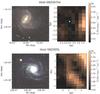 |
Fig. 1 Top and bottom: the hosts of SN 2007kk (UGC 2828) and SN 2005L (MCG+07-33-005), respectively, both classified as globally star-forming (Childress et al. 2013b). Left: color images made using observations from SNIFS and SDSS-III (Aihara et al. 2011). On both images, the field-of-view of SNIFS, centered on the SN position (white-star marker), is indicated by the orange central square. Right: Hα surface brightness maps of the SN vicinities (the generation of these maps is detailed in Sect. 2.3). SN 2007kk occurred in a passive environment more than 1.5 kpc from the closest star-forming region, while SN 2005L is located at the edge of such a region. |
In this work we analyze the host galaxy regions in the immediate vicinity for a large sample of SNe Ia from the Nearby Supernova Factory (SNfactory, Aldering et al. 2002). Our integral field spectrograph accesses the local environment of observed SNe, and therefore probes local host properties, such as gas and stellar metallicities and star formation history. While Stanishev et al. (2012) have conducted such a study by looking at the metallicity of the local environments of a sample of seven nearby SNe Ia, ours is the first such large-scale study.
Delay-time distribution studies (Scannapieco & Bildsten 2005; Mannucci et al. 2005, 2006; Sullivan et al. 2006) predict that a fraction of SNe Ia, known as “prompt” SNe, should be associated with young stellar populations. The rest, referred to as “tardy” or “delayed” SNe, should be related to older stars. Individual star-forming regions (H ii regions) have a typical lifetime of a few Myr (Alvarez et al. 2006), much shorter than expected – even for the fastest – SN Ia progenitor systems (few tens of Myr, Girardi et al. 2000). It is therefore impossible to make a physical connection between a SN and the H ii region in which its progenitor formed. However such star-forming regions are gathered in groups (see for instance M 51 in Lee et al. 2011), concentrated in spiral arms whose lifetimes are longer than the time scale for a prompt SN. (See Kauffmann et al. 2003, for details on the star formation history of galaxies.) This motivated us to employ Hα for our first analysis of SNe Ia local environments. Hα will be taken to indicate active local star formation, and thus the likelihood that a given progenitor was especially young.
Long before the “prompt” and “tardy” distinction, association with H ii regions or spiral arms was a common approach for understanding the stellar populations from which SNe formed. For instance, with small samples of SNe, Bartunov et al. (1994) and later James & Anderson (2006) showed that Type Ia SNe were less associated with such regions than are core-collapse SNe. A key ingredient missing in such studies needed to understand SNe Ia in detail is accurate standardized luminosities, which we have for our sample. Also, in light of the “prompt”/“tardy” dichotomy, it will be important to consider the possibility that SNe Ia will fall into discrete subsets based on the strength of star formation in their local environment.
After the presentation of our data (Sect. 2) and our method for quantifying neighboring star-forming activity (Sect. 3), we investigate the correlation of SNe Ia light-curve parameters with the local environment (Sect. 4). This includes a review of how our results based on the local environment compare with the aforementioned global host galaxy studies. In particular, we present evidence for excess dust obscuration of SNe Ia in actively star-forming environments. We also show that the corrected SN Ia brightnesses depend significantly on the local Hα environment. We discuss the implications of our results in Sect. 5, where the standardization of SNe Ia is examined. We then compare our local Hα analysis with previous results concerning the total host stellar mass, finding important clues to the origin of the mass step. In Sect. 6, we estimate the impact of the local trends on the cosmological parameters using a simple model, and then use this model to show redshift evolution in SNe Ia from the literature. We further demonstrate the existence of a SN Ia subset having a significantly reduced brightness dispersion. Finally, in Sect. 7 we test the robustness of our results, and end with a summary in Sect. 8.
2. Integral field spectroscopy of immediate SN Ia neighborhoods
2.1. SNIFS and the SNfactory
The SNfactory has observed a large sample of nearby SNe and their immediate surroundings
using the SuperNova Integral Field Spectrograph (SNIFS, Lantz et al. 2004) installed on the UH 2.2 m telescope (Mauna Kea). SNIFS is a
fully integrated instrument optimized for semi-automated observations of point sources on
a structured background over an extended optical window at moderate spectral resolution.
The integral field spectrograph (IFS) has a fully filled
 spectroscopic field-of-view
subdivided into a grid of 15 × 15 contiguous square spatial elements (spaxels). The
dual-channel spectrograph simultaneously covers 3200–5200 Å (B-channel)
and 5100–10 000 Å (R-channel) with 2.8 and 3.2 Å resolution,
respectively. The data reduction of the x,y,λ data cubes was summarized
by Aldering et al. (2006) and updated in Sect. 2.1
of Scalzo et al. (2010). A preview of the flux
calibration is developed in Sect. 2.2 of Pereira et al.
(2013), based on the atmospheric extinction derived in Buton et al. (2013).
spectroscopic field-of-view
subdivided into a grid of 15 × 15 contiguous square spatial elements (spaxels). The
dual-channel spectrograph simultaneously covers 3200–5200 Å (B-channel)
and 5100–10 000 Å (R-channel) with 2.8 and 3.2 Å resolution,
respectively. The data reduction of the x,y,λ data cubes was summarized
by Aldering et al. (2006) and updated in Sect. 2.1
of Scalzo et al. (2010). A preview of the flux
calibration is developed in Sect. 2.2 of Pereira et al.
(2013), based on the atmospheric extinction derived in Buton et al. (2013).
For each followed SN, the SNfactory creates a spectro-photometric time series typically composed of ~13 epochs, with the first spectrum taken on average three days before maximum light in B (Bailey et al. 2009; Chotard et al. 2011). In addition, observations are obtained at the SN location at least one year after the explosion to serve as a final reference to enable the subtraction of the underlying host. For this analysis, we gathered a subsample of 119 SNe Ia with good final references and properly measured light-curve parameters, including quality cuts suggested by Guy et al. (2010).
2.2. Local host observations
The SNfactory software pipeline provides flux-calibrated x,y,λ cubes corrected for instrumental and atmospheric responses (Buton et al. 2013). Each spaxel of an SN cube includes three components, each one characterized by its own spatial signature:
-
1.
the SN is a pure point source, located close to the centerof the SNIFS field of view (FoV);
-
2.
the night sky spectrum is a spatially flat component over the full FoV;
-
3.
the host galaxy is a (potentially) structured background.
In this section, we present the algorithm used to disentangle the three components. In Sect. 2.2.1, we describe the method used to subtract the SN component from the original cubes, and in Sect. 2.2.2 our sky-subtraction procedure, using a spectral model for the sky that prevents host-galaxy signal contamination. All cubes from the same host are finally combined to produce high signal-to-noise (S/N) cubes and spectra. This process is detailed in Sect. 2.2.3.
2.2.1. SN subtraction
The point source extraction from IFS data requires the proper subtraction of any structured background. Using a 3D deconvolution technique, Bongard et al. (2011) show how we construct a “seeing-free” galaxy x,y,λ cube from final reference exposures taken after the SN Ia has vanished (typically one year after maximum light). After proper registration and reconvolution with the appropriate seeing, this model is subtracted from each observed cube to leave the pure point-source component plus a spatial constant similar to a sky signal. Three-dimensional PSF photometry is then applied to the host-subtracted cube to extract the point source spectrum (e.g., Buton et al. 2013).
For the present local host property analysis, we went one step further and subtracted the aforementioned fitted PSF from the original cubes to obtain SN-subtracted host cubes. Figure 2 shows an example of such a subtraction procedure. Since the SNfactory acquires SN Ia time series, this technique provides as many local host observations as SN pointings (on average 13), in addition to the final references (on average 2).
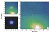 |
Fig. 2 SN subtraction from a host cube. Different reconstructed images, made by integrating x,y,λ cubes along the λ axis, are shown for a single observation of SNF20070326-012. Top left: original flux-calibrated cube containing host, sky, and SN signals. Bottom left: pure SN cube obtained after host subtraction (image) and fitted PSF model (contours). Right: SN-subtracted host cube. |
2.2.2. Sky subtraction
Since SNIFS has a FoV spanning only ~6″ across, it is usually not possible to find a region entirely free of host signal, as is usually done in photometry or long-slit spectroscopy. The night sky spectrum is a combination of the atmospheric molecular emission, zodiacal light, and scattered star light, along with the moon contribution if any (Hanuschik 2003). We have developed a sky spectrum model from a principal component analysis (PCA) on 700 pure sky spectra obtained from standard star exposures in various observing conditions. The B and R channels are analyzed independently and in slightly different ways.
The emission lines in R sky spectra (mainly oxygen and OH bands) are easily isolated from the underlying continuum. This continuum is fitted by a fourth-order Legendre polynomial over emission line-free wavelength regions. The PCA is then performed on the continuum-subtracted emission line component. Eight principal components (PCs) are necessary to reconstruct the emission spectrum with a median reduced χ2 of 1. An example of a red-sky spectrum fit using this 13-parameter model is given in Fig. 3.
The B sky spectrum is dominated by diffuse light and shows absorption features, as well as a few Herzberg O2 lines in the bluer part of the spectrum. For this channel a PCA is performed directly on the observed sky spectra, since it was not possible to disentangle the different physical components as easily as for the R sky spectra. We find that four PCs are necessary to reach a median reduced χ2 of 1.
In total, our B + R sky model is therefore described by 4 + (5 + 8) = 17 linear parameters. Since this model is trained on selected pure sky spectra, none of the PCs should mimic galactic features: even if some chemical elements are common (e.g., the hydrogen or nitrogen lines), host galactic lines are redshifted and cannot be spuriously fit by the model.
Each spaxel of the SN-subtracted cube can be decomposed as follows:  (1)where the spatially
flat sky component does not depend on the spaxel location (x,y). We
define the presumed sky as the mean spectrum of the five faintest
spaxels, i.e. with the smallest host contribution. Since the
host(x,y,λ) component of Eq. (1) may not be strictly null for these spaxels, the presumed
sky may still contain galactic features, such as hydrogen emission lines, and
cannot be used directly as a valid estimate of the true sky spectrum. We therefore fit
the presumed sky spectrum with our model: the resulting modeled sky is
free of any galactic features and can safely be subtracted from each spaxel to obtain a
pure host cube. (See Fig. 3 for an example using
the R-channel.)
(1)where the spatially
flat sky component does not depend on the spaxel location (x,y). We
define the presumed sky as the mean spectrum of the five faintest
spaxels, i.e. with the smallest host contribution. Since the
host(x,y,λ) component of Eq. (1) may not be strictly null for these spaxels, the presumed
sky may still contain galactic features, such as hydrogen emission lines, and
cannot be used directly as a valid estimate of the true sky spectrum. We therefore fit
the presumed sky spectrum with our model: the resulting modeled sky is
free of any galactic features and can safely be subtracted from each spaxel to obtain a
pure host cube. (See Fig. 3 for an example using
the R-channel.)
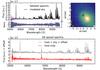 |
Fig. 3 Sky subtraction process for an R cube of host-SNF20060512-001. Top right: reconstructed image of a final reference acquisition (it could as well be an SN-subtracted cube); the central star marker indicates the SN location. The dot markers indicate the faintest spaxels used to measure the presumed sky. Top left: modeled sky (thick black) fit over the mean of the five faintest spectra (thin colored); the bottom part shows the fit residuals, compared to the presumed sky error (blue band). Bottom: host spectrum at the SN location before (upper thin gray line) and after (lower thick red line) the sky subtraction. The emission at 6830 Å is the Hα+[N ii] gas line complex, left untouched by the sky subtraction procedure. The few small features further toward the red are residuals from the sky subtraction, but this part of the spectrum is not used in this analysis. See Sect. 2.3 for details. |
This procedure could slightly overestimate the sky continuum in cases of bright host signals even in the faintest spaxels, and ultimately lead to a underestimation of the Hα flux measurements (Groves et al. 2012). This effect is, however, insignificant in comparison to our main source of Hα measurement error, related to our inability to correct for host dust extinction (see Sect. 2.3).
2.2.3. Spectral merging
In this analysis, we focus on the host properties of the SN local environment, which we define has having projected distances less than 1 kpc from the SN. This radius has been chosen since it is greater than our median seeing disk for our most distance host galaxies, at z = 0.08. (1″ = 1.03 kpc at z = 0.05.) No allowance was made for host galaxy inclination in defining this local region.
Once the SN and the sky components have been subtracted, we computed the mean host spectrum from each cube within 1 kpc around the SN. This requires precise spatial registration (a by-product of the 3D deconvolution algorithm, see Sect. 2.2.1) and atmospheric differential refraction correction. Those spectra (15 on average per SN) are then optimally averaged and merged to get one host spectrum of the local environment per SN. The spectral sampling of these merged-channel spectra is set to that of the B-channel, which is 2.38 Å. In the same fashion, we are able to combine 3D-cubes to create 2D-maps of any host property.
The spectra are corrected for Milky-Way extinction (Schlegel et al. 1998). In this paper, observed fluxes are expressed as surface brightnesses, and wavelengths are shifted to rest frame. We only consider the 89 SNe Ia in the main SNfactory redshift range 0.03 < z < 0.08 for spatial sampling reasons; namely, at lower z the final SNIFS field of view remaining after spectral merging often subtends a radius of less than 1 kpc surrounding the SN location, while at higher z the typical seeing disk subtends substantially more than 1 kpc. Since this selection is only based on redshift, it does not introduce bias with respect to host or SN Ia properties. (See Childress et al. 2013b,who showed that our host data follow regular galaxy characteristics.)
The influence of the PSF, i.e., the variation in the amount of independent information with redshift for a given kpc-radius aperture, is discussed in Sect. 7, where we show that our analysis is free of any redshift bias.
2.3. Measurement of the local host properties
A galactic spectrum is a combination of a continuum component with absorption lines mostly from the stars and emission lines from the interstellar gas. In this paper, we restrict our analysis to the Hα signal around the SN. Since hydrogen emission line intensities can be affected by underlying stellar absorption, it is necessary to estimate the stellar continuum to obtain accurate Hα measurements. (See Fig. 4.)
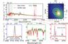 |
Fig. 4 Spectral fit of the host mean spectrum in the projected 1 kpc radius around SNF20060512-001. Top right: reconstructed image of a final reference exposure. The circle aperture shows the 1 kpc aperture centered on the SN location (central star marker). Top left: mean host spectrum within 1 kpc radius around the SN (rest-frame, green dashed-line with ± 1σ error band), averaged over 21 cubes (including two final references). The best ULySS fit is shown as the sum of a stellar continuum (red line) and gas lines (magenta dashed line). Bottom, from left to right: zoom on [O ii]λλ3726,3728, 4000 Å break, and Hα + [N ii]λλ6548,6584 + [S ii]λλ6716,6731 wavelength regions. |
The University of Lyon Spectroscopic analysis Software1 (ULySS, Koleva et al. 2008, 2009) is used to disentangle the stellar and gas components. It fits the following three components simultaneously: stellar populations from the MILES library (Sánchez-Blázquez et al. 2006); a set of emissions lines – Balmer’s hydrogen series in addition to [O ii]λλ3726,3728, [O iii], [N ii], and [S ii]; and a multiplicative ad hoc continuum correcting for both internal dust extinction and any remaining large-scale flux mismatch between the data and the template library. Only wavelengths matching the MILES library rest frame are considered (3540–7410 Å), and gas emission lines all share a common redshift and velocity dispersion. Because of this added constraint, gas emission flux uncertainties given by ULySS cannot be trusted readily. We therefore ultimately fit Gaussian profiles on stellar-corrected emission lines to derive Hα fluxes and accurate uncertainties.
Figure 4 presents the fit of the mean spectrum of the local environment for SNF20060512-001. In this particular case 21 exposures per channel, including two final references, have been combined. The stellar component is strongly constrained by the D4000 feature, and thereby gas flux measurements properly account for stellar absorption.
In this paper, we focus our study on the Hα line as a tracer of the star-forming activity (Kennicutt 1998). The spectra are not corrected for the internal host extinction, because the Balmer decrement method (Calzetti et al. 1994) cannot be reliably applied: the Hγ lines are usually too faint, and Hβ lines happen to lie at the SNIFS dichroic cross-over (4950 < λ < 5150 Å in the observer frame, see Fig. 4), where the S/N is low and fluxes harder to calibrate.
3. Local Hα surface brightness analysis
The Hα emission within a 1 kpc projected radius can be conveniently recast as a surface brightness, which we designate with ΣHα. Because the measurement is projected, it actually represents the total Hα emission in a 1 kpc radius column passing through the host galaxy centered on the SN position. Thus, it is possible that Hα we detect, in whole or in part, is in the foreground or background of the 1 kpc radius sphere surrounding the SN.
However, there are several factors that greatly suppress projection effects for Hα relative to stars. One is that Hα depends on the square of the electron density, so most Hα comes from those rare regions with high gas density. This advantage is compounded by the fact that young stars capable of ionizing hydrogen also tend to occur in clumps and regions of higher gas density (see Kennicutt & Evans 2012, especially Sect. 2.2, for a detailed discussion of H ii regions and their clumpiness). In addition, while stars are spread across thin and thick disks, bulges and halos, H ii regions are concentrated in the thin galactic disk, where a typical scale height is only ~0.1 kpc (Paladini et al. 2004). Thus the line-of-sight depth extends beyond our canonical 1 kpc radius only for very high inclinations (i.e., i > 84deg). Finally, the Hα covering fraction is generally low because H ii regions are so short-lived (see Calzetti 2012, for a detailed review of tracers of star formation activity.).
Definition of the two ΣHα subgroups, and their respective weighted mean light-curve parameters.
In the following analysis, a few cases (7/89) of SNe with locations projected close to the core of very inclined hosts have been set aside because of the high probability of such misassociation (designated as “p.m.s.”, see Table 1). In Sect. 7 we show that these cases have no influence on our results.
A different projection effect occurs if SNe Ia travel far from their formation environment before they explode. Owing to random stellar motions this will occur, and its importance will itself depend on SNe Ia lifetimes and the host velocity dispersion. If as expected, tardy SNe Ia are associated with old stellar populations, this correspondence may be lost only in cases where the host is globally star forming – i.e., for spiral rather than elliptical galaxies – and the SN motion has projected it onto a region of active star formation. As with the line-of-sight projection discussed above, this situation should be uncommon. On the other hand, prompt progenitors should not have drifted from their stellar cohort by more than our fiducial 1 kpc radius. This cohort is likely to have been an open cluster or OB association; open clusters remain bound on the relevant timescale, while OB associations have very low velocities dispersions (~3 km s-1de Zeeuw et al. 1999; Portegies Zwart et al. 2010; Röser et al. 2010). Consequently, there should be little contamination due to this type of projection effect for young progenitors.
Thus, the net effect will be that for some old SN progenitors in globally star-forming galaxies a false positive association with Hα may arise from these projection effects. However, we expect the number of such cases to be small, as discussed later in this section.
For ease in interpretation, we split our sample in two, using the median ΣHα value of our distribution, log (ΣHα) = 38.35, as the division point. This corresponds to a star formation surface density of 1.22 × 10⁻³M⊙ yr-1 kpc-2 assuming Eq. (5) of Calzetti et al. (2010). Cases where no Hα signal was found are arbitrarily set to log (ΣHα) = 37 in the figures.
The median ΣHα value happens to correspond to the threshold at which we achieve a minimal 3σ-level measurement sensitivity. It also corresponds to the mean log (ΣHα) of the warm interstellar medium (WIM) distribution reported by Oey et al. (2007). The source of the WIM is controversial. The long-standing interpretation has been that the WIM is due to Lyman continuum photons that have escaped from star-forming regions and then ionize the ISM. In this interpretation, the WIM would still trace star formation, but its distribution would be more diffuse than an H ii region. This distinction would not matter given our large metric aperture since even in the ISM the optical depth to Lyman continuum photons is large. Recently, however, Seon & Witt (2012) have interpreted the WIM as due to reflection of light from H ii regions off of ISM dust. In this case WIM Hα would still arise from star formation, but possibly from distances well outside our metric aperture since the optical depth to Hα photons can be low. By setting our division point above the nominal log (ΣHα) of the WIM we minimize the importance of these details for our analysis.
We designate these two ΣHα subgroups as follows (see Table 1):
-
41 SNe Iaα withlog (ΣHα) ≥ 38.35, which we refer to as “locally star forming”,
-
41 SNe Iaϵ with log (ΣHα) < 38.35, which we refer to as “locally passive”.
Figure 5 presents a quantitative picture of the point made visually in Fig. 1 by illustrating the non-trivial relationship between local and global measurements for cases considered passive. The global quantities for our hosts are taken from our compilation in Childress et al. (2013b); in three cases, global host sSFR measurements are unavailable for SNe Ia in our local environment sample. Figure 5 shows that half of the SNe with locally passive environments (20/38) have a globally star-forming host (traditionally defined as log (sSFR) > −10.5). This highlights the existing degeneracy when employing global properties: the SNe Ia hosted in star-forming galaxies can have either star-forming or passive local environments whereas SNe hosted in passive galaxies are almost certain to have a locally passive environment.
With ΣHα above the median value, SNe Iaα are most likely to have young progenitors since an Hα signal has been positively detected in their vicinities. The large number of SNe Ia with detections of local star formation in Fig. 5 itself provides an indication that young progenitors exist, in agreement with the statistical analysis of Aubourg et al. (2008). On the other hand, the wide range of observed ΣHα is an indication of SNe from both passive and star-forming regions, i.e. from both young and old progenitors (Scannapieco & Bildsten 2005; Mannucci et al. 2005, 2006; Sullivan et al. 2006).
In Fig. 5 there is a relative dearth of SNe Ia with Hα detections for log (ΣHα) < 37.9 in hosts that are globally star-forming. This then highlights a population having 38.0 < log (ΣHα) < 38.35 in globally star-forming hosts that are counted as locally passive when we split our sample. Their proximity to the typical WIM level suggests that these could be cases of SNe Ia from old progenitors whose ΣHα value is boosted by projection onto the WIM in their hosts. But, they may equally well be SNe Ia from young/intermediate age progenitors where strong star formation has already ebbed at that location in their host. In Sect. 7 we show that moving these cases into the star-forming sample does not change our results significantly. Therefore we prefer to employ a simple split since it is not tuned to any patterns in the data.
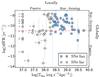 |
Fig. 5 Local vs. global star-forming environment. Blue squares and open-circles show the SNe Ia from locally star-forming and passive regions, respectively (log (ΣHα) ≷ 38.35, blue-dotted line). Gray arrows indicate points with ΣHα signals compatible with zero (detection at less than 2σ). The red-dashed line indicates the limit that is commonly used to distinguish between star-forming and passive galaxies when using global host galaxy measurements (log (sSFR) ≷ −10.5). Three SNe Ia from our sample do not have sSFR measurements. |
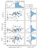 |
Fig. 6 SN Ia parameters as a function of log (ΣHα), the surface
brightness in the 1 kpc radius around the SNe Ia. Upper panel: the
log (ΣHα) distribution colored with respect to
ΣHα subgroups: Iaϵ and
Iaα are shown as empty-black and filled-blue histograms,
respectively. Main panels, from top to bottom: SALT2 stretch
x1, color c, and the Hubble residuals
corrected for stretch and color |
4. ΣHα and SN Ia light-curve properties
We now compare log (ΣHα) to the SN light-curve parameters
(Sect. 4.1) and to the corrected Hubble residuals
 (Sect. 4.2). We show that SNe from locally passive regions have
faster light-curve decline rates, that the color of SNe Ia is correlated with
ΣHα, and that there is a significant magnitude offset
between SNe from locally star-forming (Iaα) and locally passive
(Iaϵ) regions.
(Sect. 4.2). We show that SNe from locally passive regions have
faster light-curve decline rates, that the color of SNe Ia is correlated with
ΣHα, and that there is a significant magnitude offset
between SNe from locally star-forming (Iaα) and locally passive
(Iaϵ) regions.
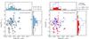 |
Fig. 7 SALT2 stretch x1 vs. color c. Left: the local perspective. SNe markers and x1 and c marginalized stacked distributions follow the same color-shape code as Fig. 6. Right: the global perspective. Open-blue squares show the globally star-forming hosts and red dots show the globally passive hosts (log (sSFR) ≶ −10.5 respectively). Big markers indicate SNe with local measurements, while small markers denote SNe not in our local sample (failed redshift cut, but passed the quality cuts, see Sect. 2.1). Stacked histograms are the marginalized distributions of x1 and c using the marker color codes. These figures compare to Fig. 2 of Lampeitl et al. (2010). Notice the mix of local environments for moderate x1 while low x1 are almost exclusively from passive environments. |
The SALT2 light-curve parameters c and x1 are
known to correlate with the uncorrected absolute B-magnitude at maximum
light, MB. The dispersion in
MB can be reduced significantly by taking
advantage of these correlations (Guy et al. 2007):
 (2)where the stretch
coefficient α, the color coefficient β, and the average
absolute magnitude of the SNe Ia,
(2)where the stretch
coefficient α, the color coefficient β, and the average
absolute magnitude of the SNe Ia,  , are
simultaneously fit over the SN sample during the standardization process. The SALT
light-curve parameters and Hubble residuals for our SNe Ia have been presented previously in
Bailey et al. (2009), Chotard et al. (2011), and Childress et
al. (2013a).
, are
simultaneously fit over the SN sample during the standardization process. The SALT
light-curve parameters and Hubble residuals for our SNe Ia have been presented previously in
Bailey et al. (2009), Chotard et al. (2011), and Childress et
al. (2013a).
For the statistical analyses that follow we use the Kolmogorov-Smirnov test (KS-test) to
estimate the discrepancy between observed parameter distributions
(x1, c, and
). We also
compare the weighted-mean values of those distributions between the
ΣHα groups, which we denote using the form
δ ⟨ X ⟩ (A − B) ≡ ⟨ X ⟩ A − ⟨ X ⟩ B.
When exploring correlations we employ the non-parametric Spearman rank correlation test,
quoting the correlation strength, rS, and probability,
pS. p-values below 5% (e.g.,
pKS < 0.05) highlight
statistically important differences between distributions, and we will consider
p-values below 1% to be highly significant.
4.1. Light-curve stretch and color
The stretch parameter x1 and color c are shown in Fig. 6 as a function of log (ΣHα). The weighted means and dispersions for the two subgroups are summarized in Table 1.
4.1.1. The light-curve stretch
The SALT2 stretch x1 and the log (ΣHα) values are correlated, as demonstrated by a highly significant Spearman rank correlation coefficient: rs = 0.42, ps = 7.4 × 10⁻⁵, 4.2σ. This shows that SNe Ia from low ΣHα environments have on average faster light-curve decline rates. When comparing ΣHα subgroups, we find δ ⟨ x1 ⟩ (Iaα − Iaϵ) = 0.37 ± 0.17 (pKS = 5.8 × 10⁻³).
At first this might appear to be just the same as the well-established effect whereby globally passive galaxies are found to host SNe Ia with lower stretch, while star-forming host galaxies dominate at moderate stretches (Hamuy et al. 2000; Neill et al. 2009; Lampeitl et al. 2010). Indeed, the x1 distributions of SNe in globally passive and star-forming hosts (log (sSFR) ≶ −10.52) differ significantly, having pKS = 2.0 × 10⁻³ for the SNfactory and pKS = 10-7 for SDSS (Lampeitl et al. 2010). We compare in Fig. 7 the global and local pictures in the (c,x1) plane. These two figures can be compared to Fig. 2 of Lampeitl et al. (2010) for the SDSS sample.
However, our analysis of the local environment displays quite a different stretch distribution for passive environments. We find that 40% of SNe that are locally passive have moderate stretches. This is in strong contrast to global analyses. For our SN sample only 25% of globally passive hosts have SNe Ia with x1 > −1, and in the global analysis of the SDSS dataset Lampeitl et al. (2010) the percentage of passive environments with moderate stretch is even lower, a mere 11%. This suggests that many SNe Ia originating in passive environments have been mistakenly categorized as coming from star-forming environments by analyses employing galactic properties integrated over the entire host. Were we to lower our dividing line to log (ΣHα) = 38, our global and local analyses would then agree, but this still would not result in the paucity of passive environments at moderate stretches seen in the SDSS sample.
Furthermore, we find even stronger evidence that SNe with fast decline rates (x1 < −1) arise in passive environments. In our local analysis 15/18, or 83% are Iaϵ, and all have a log (ΣHα) ≤ 39. In contrast, as Fig. 7 shows, our global analysis for x1 < −1 shows only mild dominance by passive galaxies, with 60% being such hosts. In the SDSS sample of Lampeitl et al. (2010), among the SNe Ia with fast decline rates only 54% are globally passive.
In summary, we find that lower stretch SNe Ia are hosted almost exclusively in passive local environments, but that SNe Ia having moderate stretches are hosted by all types of environments.
4.1.2. The light-curve color
We also find that SNe Ia from star-forming environments are on average redder than those from passive environments at the 2.2σ level: δ ⟨ c ⟩ (Iaα − Iaϵ) = 0.036 ± 0.017 (0.031 ± 0.015 when removing the reddest, SNF20071015-000). This effect is more significant when comparing the tails of the log (ΣHα) distribution (lower and upper quartiles), where we find distribution differences with pKS = 0.026. As seen in Fig. 6, the SALT2 color, c, and the log (ΣHα) values are correlated, with a 2.0σ non-zero Spearman rank correlation coefficient rs = 0.21, with ps = 0.054.
Since dust is associated with active star formation (e.g. Charlot & Fall 2000), a color excess is expected for SNe Ia in strong ΣHα environments. (See Chotard et al. 2011, for a discussion of the Type Ia color issue.) This trend has been suggested for SNLS SNe in Sullivan et al. (2010) but is not seen in SDSS data (Lampeitl et al. 2010).
As discussed earlier, by analyzing integrated galaxy properties, global host studies merge SNe Iaϵ with x1 > −1, and the SNe Iaα, into a single star-forming host category. Figure 7 shows that low and moderate stretch Iaϵ share the same color distribution. It is then difficult for global analyses to detect the color variation between the star-forming and passive hosts, since both kinds harbor some Iaϵ. Indeed, in the SNfactory sample globally passive and star-forming hosts produce SNe Ia having the same SALT2 color distribution (pKS = 0.654).
4.2. Hubble residuals
The SALT2 raw Hubble residuals ΔMB are
corrected for their stretch and color dependencies
() and are
shown in Fig. 6 as a function of
log (ΣHα). The weighted mean values per
ΣHα group are summarized in Table 1.
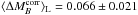
4.2.1. The Hα bias
We find with a 3.1σ significance that SNe from locally passive
environments are brighter than those SNe Ia in locally star-forming environments after
color and stretch correction:  mag (pKS = 0.012). The amplitude of this
significant brightness offset – hereafter called the “Hα bias” – is a
concern for precision cosmology, since the fraction of SNe Ia from passive environments
most likely evolves with redshift, thus creating a redshift dependence on the average
SNe Ia luminosity. Distance measurements to these standardizable candles are therefore
biased. A more complete discussion of the potential impact on cosmological measurements
is presented in Sect. 6.
mag (pKS = 0.012). The amplitude of this
significant brightness offset – hereafter called the “Hα bias” – is a
concern for precision cosmology, since the fraction of SNe Ia from passive environments
most likely evolves with redshift, thus creating a redshift dependence on the average
SNe Ia luminosity. Distance measurements to these standardizable candles are therefore
biased. A more complete discussion of the potential impact on cosmological measurements
is presented in Sect. 6.
4.2.2. Corrected Hubble residual distributions
We now investigate the possible origin of this brightness offset between the SNe
Iaα and the SNe Iaϵ (Hα bias) by
examining the
distributions of each subgroup. In Fig. 6 we notice
the presence of a subgroup of significantly brighter SNe hosted exclusively in locally
passive environments. We thus distinguish two modes in the distribution of corrected
Hubble residuals: (1) The first mode exists in all environments and has
 . (2) The second mode is
exclusive to SNe Ia from low Hα environments (Iaϵ),
and it populates the brighter part of the diagram almost exclusively: among the 20 SNe
Ia with
. (2) The second mode is
exclusive to SNe Ia from low Hα environments (Iaϵ),
and it populates the brighter part of the diagram almost exclusively: among the 20 SNe
Ia with  , 17
are Iaϵ, and only one has a
log (ΣHα) > 39. For analysis
purposes we define and label these modes as follows:
, 17
are Iaϵ, and only one has a
log (ΣHα) > 39. For analysis
purposes we define and label these modes as follows:
-
Mode 1 (M1): 65 SNeconsisting of all SNe Iaαalong with SNe Iaϵ that have
 mag.
mag. -
Mode 2 (M2): 17 SNe Iaϵ with
mag.
Except that both are from locally passive environments, the M2 subgroup and the subgroup of 15 fast declining (x1 < −1) SNe Ia turn out to not be directly related, having only six SNe in common.
Figure 8 shows the distribution of these two modes
fitted by normal distributions (with 3σ clipping). The
M1 SNe are on average fainter
( mag) and M2 SNe Ia are brighter
(
mag) and M2 SNe Ia are brighter
( mag) than the full sample.
The standard deviations are 0.099 ± 0.009 mag and 0.060 ± 0.010 mag for
M1 and M2, respectively. The
weighted RMS gives similar results, with variations at a tenth of the error level. With
no clipping, one additional, bright SN is then retained in
M1, raising the M1 standard
deviation to 0.113 ± 0.010 mag.
mag) than the full sample.
The standard deviations are 0.099 ± 0.009 mag and 0.060 ± 0.010 mag for
M1 and M2, respectively. The
weighted RMS gives similar results, with variations at a tenth of the error level. With
no clipping, one additional, bright SN is then retained in
M1, raising the M1 standard
deviation to 0.113 ± 0.010 mag.
These differences in  would appear to be extremely
significant; however, in this case we chose the dividing point in
, and
thus the added degrees of freedom are not accounted for. To better assess the
significance of the bimodal structure we use the Akaike Information Criterion corrected
for finite sample size (AICc; Burnham & Anderson
2002). When comparing two models, the one with the smallest AICc provides a
better fit to the data. The AICc test is similar to a maximum likelihood ratio that
penalizes additional parameters.
would appear to be extremely
significant; however, in this case we chose the dividing point in
, and
thus the added degrees of freedom are not accounted for. To better assess the
significance of the bimodal structure we use the Akaike Information Criterion corrected
for finite sample size (AICc; Burnham & Anderson
2002). When comparing two models, the one with the smallest AICc provides a
better fit to the data. The AICc test is similar to a maximum likelihood ratio that
penalizes additional parameters.
The two models that we compare are the following: (1) The reference model is a regular normal distribution, with two parameters: a mean and an intrinsic dispersion. (2) The alternative model is bimodal with three parameters: two means and the ratio of the two mode amplitudes. In the bimodal model no intrinsic dispersion is needed, because the SALT2 and peculiar velocity uncertainties are able to fully explain the dispersion of each mode. In both cases the integral of the model is required to equal the number of SNe used in the fit. For the full sample we find ΔAICc(bimodal - unimodal) = −5.6, which strongly favors the bimodal structure. If we remove the possibly contaminated “p.m.s.” cases we find a slightly reduced value of ΔAICc(bimodal - unimodal) = −4.3. Thus, whether we include these or not has little impact. The fact that the bimodal model does not require the introduction of an ad hoc intrinsic dispersion lends it further weight.
In addition we have tested for bimodality in the Hubble residuals for the locally
passive subset alone. Here the first normal mode is forced to match the mean
of the
Iaα subset (μ1 = 0.056), while the mean
of second normal mode and the ratio of the two mode amplitudes are free parameters. Here
again there is no need to include intrinsic dispersion, so there are only two
parameters. When comparing those two models, ΔAICc(bimodal–unimodal) = −3.5, which
again favors the bimodal structure, though less strongly.
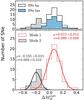 |
Fig. 8 Distribution of corrected Hubble residuals per ΣHα
group (top, as in Fig. 6)
and per mode (bottom) for the full sample. In the lower panel,
the open-red and the filled-gray histograms represent the corrected Hubble
residual distributions of M1 and
M2, respectively. By definition of the modes, the
red histogram corresponds to the stack of the blue distribution with the open
histogram above |

In Sect. 5.2.2 we show how this peculiar structure introduces the brightness offset observed between SNe in low- and high-mass hosts. This “mass step” is seen in our sample (Childress et al. 2013a), as well as in all other large surveys (Kelly et al. 2010; Sullivan et al. 2010; Gupta et al. 2011; Johansson et al. 2013). This suggests that this bimodality is not exclusive to the SNfactory data, but is an intrinsic property of SALT2-calibrated SNe Ia. That it has not been noticed before is very likely due to the rarity of SNe Ia having all of the necessary ingredients: well-measured light curves, small uncertainties due to peculiar velocities, and a wide range of ΣHα, and/or total stellar mass.
5. Discussion
Here we discuss the results presented previously. First, we look for the potential environmental dependency of stretch and color coefficients among the two ΣHα subgroups (Sect. 5.1). Next, we investigate the previously-observed relations between host masses and both the SNe stretches (Sect. 5.2.1) and the SNe-corrected Hubble residuals (Sect. 5.2.2). These relations are interpreted from our local analysis perspective.
5.1. The standardization process
Since the distributions of SN Ia parameters have been shown to vary between our two ΣHα subgroups, we now investigate whether a unique standardization process applies in the context of SALT2 by comparing stretch and color coefficients (α and β respectively; see Eq. (2)) between the ΣHα subgroups. We find that the stretch coefficient, α, is consistent between ΣHα groups, having δα(Iaα − Iaϵ) = −0.020 ± 0.037.
The color coefficient of SNe between low-and high-ΣHα differ by δβ(Iaα − Iaϵ) = 1.0 ± 0.41, but this difference is dominated by the reddest SN, SNF20071015-000. After removing it, the color coefficients are not significantly different: δβ(Iaα − Iaϵ) = 0.67 ± 0.45. Therefore, our analysis is insensitive to any color coefficient variations between ΣHα groups. The color of the outlier, SNF20071015-000, is likely to be dominated by dust, for which a larger color coefficient is expected, as we have shown in Chotard et al. (2011).
We also measured what influence the lowest-stretch SNe Iaϵ from passive
environments may have on the existence of the brighter M2
mode. Our sample contains 15 Iaϵ with
x1 < − 1; we performed an
independent standardization on the remaining 67 SNe, among which 26 are
Iaϵ, 11 of which have  . This fraction, 11
M2/26 Iaϵ, is exactly the same as that
computed from the full sample (17/41). Therefore, we conclude that the existence of the
M2 mode is unrelated to the presence of a fast decline rate
subgroup in passive environments.
. This fraction, 11
M2/26 Iaϵ, is exactly the same as that
computed from the full sample (17/41). Therefore, we conclude that the existence of the
M2 mode is unrelated to the presence of a fast decline rate
subgroup in passive environments.
5.2. Host mass vs. SN properties: A local environment perspective
We investigate here the correlations found by global host studies between total host stellar mass and both the stretch and the SN-corrected Hubble residuals (Kelly et al. 2010; Sullivan et al. 2010; Gupta et al. 2011; Childress et al. 2013a; Johansson et al. 2013).
5.2.1. Mass-stretch correlation
Stretch has been shown to correlate with the host’s stellar mass (e.g., Sullivan et al. 2010). Figure 9 shows x1 as a function of host mass for our sample (see Childress et al. 2013a, for details on the SNfactory host mass analysis). In agreement with the literature, we find a correlation between mass and stretch when all the SNe Ia are considered together, with a Spearman rank correlation coefficient that is non-zero at the 3.4σ level (rs = −0.36, ps = 9.2 × 10⁻⁴).
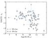 |
Fig. 9 SN Ia x1 vs. total host stellar mass (Childress et al. 2013a). Markers follow the same color and shape code as in Fig. 6. Note the distinctive “L”-shaped distribution of the SNe Iaϵ. |
When looking at ΣHα subgroups, though, we notice that SNe Ia from locally star-forming environments (Iaα) show no correlation between their stretch and the mass of their host (rs = −0.02 ; ps = 0.89). The original correlation is actually driven by SN Iaϵ from locally passive environments (rs = −0.55; ps = 4.8 × 10⁻³, a 3.0σ significance). More precisely, the correlation appears to arise from the bimodal x1 structure of this subgroup, which we previously noted in Fig. 6. Figure 9 clearly shows that the correlation is related to the L-shaped distribution of SNe Iaϵ in the x1–mass plane: SNe with x1 > −1 contribute to the whole range of host masses, whereas the ones with x1 < −1 arise exclusively in massive galaxies (log (M/M⊙) > 10).
Measurements of the local environment indicate that the light-curve widths of SNe in locally star-forming regions are independent of the total stellar mass of their hosts. For SNe Iaϵ, the total stellar mass of the host is not a stretch proxy as suggested by Sullivan et al. (2010) but an indicator of whether the two stretch subgroups (x1 ≶ −1) are represented or not. From this new perspective, the mass-stretch correlation shown in Fig. 2 of Sullivan et al. (2010) could be re-interpreted as being driven by a relatively independent grouping of SNe having higher masses (log (M/M⊙) > 10.2) and lower stretches (s < 0.9 ~ x1 < −1; Guy et al. 2007).
5.2.2. The “mass step”
The second known correlation between host masses and SNe Ia properties is an offset in
corrected Hubble residuals between SNe hosted by high-mass galaxies (brighter) and those
from low-mass hosts (fainter). This can be seen in Fig. 10. This mass effect has been observed by all of the large SNe Ia surveys
(Kelly et al. 2010; Sullivan et al. 2010; Gupta et al.
2011; Childress et al. 2013a; Johansson et al. 2013), and compiled in Childress et al. (2013a). Hereafter, we use the term
“plateau” to denote the averaged values
for SNe from either high- (H) or low-mass (L) galaxies, with a dividing point set at
log (M/M⊙) = 10. In
Childress et al. (2013a), we showed that such a
step function is a very good description of the data. We refer to the difference in the
brightness of these two plateaus as the “mass step.” For our subset of the SNfactory
sample this offset reaches  mag.
mag.
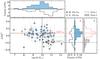 |
Fig. 10 Corrected Hubble residuals as a function of the total host stellar mass, showing
the mass step. Markers follow the same color and shape code as in Fig. 6. Top: total host stellar mass
distribution per ΣHα subgroup. Right:
|
We notice in Fig. 10 (see also Fig. 2 of Childress et al. 2013a) that the upper part of the
envelope of the distribution is constant with mass, whereas the lower part of the
distribution extends to bright values
for masses above
log (M/M⊙) ~ 10. We
see that the high-mass plateau is brighter only because a subgroup of bright SNe exists
in massive hosts. A similar trend can be observed in Fig. 4 of Sullivan et al. (2010) for SNLS, in Fig. 15 of Johansson et al. (2013) for SDSS, and in Fig. 5 of Childress et al. (2013a) where we combined all
available data.
We see in the top panel of Fig. 10 that the local
Hα environment changes with the total stellar mass of the host. For
low masses up to
log (M/M⊙) ≲ 10,
locally star-forming environments dominate (23 Iaα/34). In more massive
hosts (log (M/M⊙) ≳ 10),
however, the local SN environment presents a marked change, and the locally passive
cases are favored (27 Iaϵ/45). Since only a few
M2 SNe Iaϵ are present in lower mass
hosts (3 M2/34), the first plateau happens to be equal to
the mean M1 value, with
 .
In the upper mass range, because of the rise of the Iaϵ subgroup
populating the brighter M2 mode, the average brightness
increases up to the level of the second plateau. The Iaα population
shows no appreciable mass step; we find
.
In the upper mass range, because of the rise of the Iaϵ subgroup
populating the brighter M2 mode, the average brightness
increases up to the level of the second plateau. The Iaα population
shows no appreciable mass step; we find  ,
largely driven by the bright SNF20070701-005. There is a strong possibility that this SN
Ia is a false-positive Hα association (see Sect. 6.2), and if we remove it we find
,
largely driven by the bright SNF20070701-005. There is a strong possibility that this SN
Ia is a false-positive Hα association (see Sect. 6.2), and if we remove it we find
 .
We conclude therefore that the existence of a brighter mode, completely
dominated by SNe having locally passive environments, causes both the
Hα bias and the mass step.
.
We conclude therefore that the existence of a brighter mode, completely
dominated by SNe having locally passive environments, causes both the
Hα bias and the mass step.
6. Consequences for cosmology
The proportion of SNe from locally passive environments has surely changed with time, so the fraction of M2 SNe will depend on redshift, leading us to expect the amplitude of the mass step will change as well. In this section we develop a first estimate of this evolution bias and its consequence for measuring cosmological parameters. In Sect. 6.1, we predict the redshift dependence of the magnitude bias due to evolution in the relative numbers of SNe Iaα and SNe Iaϵ given the Hα bias we observe. We then estimate the bias on measurement of the dark energy equation of state parameter, w, that would result if this evolution does indeed occur. By then coupling the Hα bias and the mass step as discussed in Sect. 6.1.2, we verify the predicted evolution of the mass step using data from the literature. In Sect. 6.2, we introduce a subclass of SNe whose Hubble-residual dispersion is significantly reduced by avoiding this bimodality. We discuss possible strategies for mitigating this bias in Sect. 6.3.
6.1. Evolution of the SNe Ia magnitude with redshift
6.1.1. Evolution model
The mean sSFR is known to increase with redshift (e.g. Pérez-González et al. 2008), which most likely decreases the proportion of SNe associated with locally passive environments (Sullivan et al. 2006; Hopkins & Beacom 2006). Because of the Hα bias, the average SN brightness is expected to be redshift dependent.
We define ψ(z) as the fraction of SNe located in
locally passive environments (Iaϵ) as a function of redshift. Assuming
that the brightness offset between Iaα and Iaϵ is
constant with redshift, the mean corrected B-magnitude of SNe Ia at
maximum light can then be written as 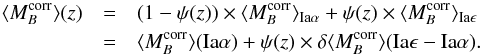 (3)Pérez-González et al. (2008) demonstrate that the
global galactic sSFR increases by a factor of ~40 between z = 0 and 2
(see also Damen et al. 2009). This evolution can
be adequately approximated as
(3)Pérez-González et al. (2008) demonstrate that the
global galactic sSFR increases by a factor of ~40 between z = 0 and 2
(see also Damen et al. 2009). This evolution can
be adequately approximated as  (4)Since sSFR
measures the fraction of young stars in a galaxy, we suggest as a toy model that the
proportion of SNe from locally passive environments evolves in complement (Sullivan et al. 2006) and therefore decreases with
z:
(4)Since sSFR
measures the fraction of young stars in a galaxy, we suggest as a toy model that the
proportion of SNe from locally passive environments evolves in complement (Sullivan et al. 2006) and therefore decreases with
z: 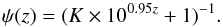 (5)From the definition of
the Iaα/Iaϵ subgroups, the SNfactory sample sets the
normalization to
ψ(z = 0.05) = 41/82 = 50 ± 5%
(Cameron 2011); hence
K = 0.90 ± 0.15.
(5)From the definition of
the Iaα/Iaϵ subgroups, the SNfactory sample sets the
normalization to
ψ(z = 0.05) = 41/82 = 50 ± 5%
(Cameron 2011); hence
K = 0.90 ± 0.15.
Then, using SN, CMB, BAO, and H0 constraints as in Suzuki et al. (2012), along with the assumption that the Universe is flat, we estimate the impact of a bias in SN Ia luminosity distance measurements. Relative to existing SN cosmological fits, we find that shifting the SN Ia luminosity distances according Eqs. (3) and (5) would shift the estimate of the dark energy equation of state by Δw ≈ −0.06 (Rubin, priv. comm., as estimated using the Union machinery, Kowalski et al. 2008; Amanullah et al. 2010; Suzuki et al. 2012).
6.1.2. Prediction of the mass step evolution
The Hα bias is due to a brightness offset between SNe Ia from locally star-forming and locally passive environments. Guided by Fig. 10, in Sect. 5.2.2, we then made a connection between the Hα bias and the mass step by noting the strong change in the proportion of SNe Iaα and SNe Iaϵ on either side of the canonical mass division at log (M/M⊙) = 10.
In Appendix A the mathematical connection between the Hα bias and the amplitude of the mass step is laid out. To a good approximation, the near absence of bright SNe Iaϵ among low-mass hosts means that the low-mass plateau is equal to the average magnitude of the SNe Iaα, and is therefore constant with redshift. By contrast, the brighter high-mass plateau has been shown to arise from a subgroup of bright SNe Iaϵ; thus, the amplitude of the mass-step will evolve along with the fraction of SNe Iaϵ, as given by ψ(z).
Thus, while local Hα measurements are not available for high-redshift
SNe Ia in the literature, our hypothesis – that the redshift evolution of the fraction
of SNe Iaϵ induces a reduction of the influence of the bright SNe that
creates both the mass step and the Hα bias – can be tested using the
same evolutionary form, ψ(z). We consequently predict
(see Appendix A.2) that the amplitude of the
mass-step,  , evolves as
 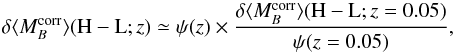 (6)where setting the
constant term,
(6)where setting the
constant term, 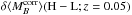 , equal to our measured mass
step provides the normalization.
, equal to our measured mass
step provides the normalization.
6.1.3. Verification of mass-step evolution
Figure 11 shows the predicted redshift evolution of the amplitude of the mass step when assuming our simple SNfactory-normalized model. We compare this model to mass steps measured using literature SNe from SNLS, SDSS, and non-SNfactory low-z datasets (Sullivan et al. 2010; Gupta et al. 2011; Kelly et al. 2010, respectively) from the combined dataset of Childress et al. (2013a). We split those data into four redshift bins with equal numbers of SNe Ia (≈120 SNe Ia in z < 0.18, 0.18 < z < 0.31, 0.31 < z < 0.6 and 0.6 < z ranges), and we measured the magnitude offset between SNe in low- and high-mass hosts assuming a step located at log (M/M⊙) = 10. Figure 11 shows that our simple model qualitatively reproduces the measured mass-step evolution with redshift. Compared to a fixed mass-step anchored by the SNfactory data, our model gives Δχ2 = −5.7 for the literature datasets. This provides external confirmation of behavior consistent with the Hα bias at greater than 98% confidence.
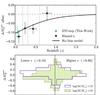 |
Fig. 11 Observed and predicted redshift evolution of the
|
6.1.4. Interpretation and Literature Corrections
From this observation we draw several conclusions. (1) The amplitude of the mass step indeed decreases at higher redshift, so host mass cannot be used as a third SN standardization parameter in the manner it has been (Lampeitl et al. 2010; Sullivan et al. 2010). (2) The observed mass steps follow the predicted evolution based on the Hα bias quite well. This in turn lends further support to the idea that the Hα bias is the origin of the magnitude offset with host mass. As the mass-step bias is observed in different datasets, the Hα bias appears to be a fundamental property of SNe Ia standardized using SALT2. (3) Any ad hoc correction of the mass step by letting SNe Ia from low- and high-mass hosts have different absolute magnitudes will be inappropriate since this assumes that high-mass hosted SNe are brighter in a constant way (Conley et al. 2011), ignoring the observed redshift evolution. Doing so will bias the SN Iaα population from high-mass hosts that dominate at higher z and miss the observed evolution of mean SNe Ia magnitude. Therefore, such a correction will not remove the bias on the dark energy equation of state, which we estimate to be Δw ~ 0.06.
Of course application of a fixed mass-step correction remains useful for bringing into agreement two datasets at the same redshift that have different proportions of low-mass and high-mass host galaxies due to survey selection effects. Whether a correction using a fixed mass step might accidentally help or hurt in correcting the redshift evolution of the Hα bias depends on the – currently unknown – correlation of the parameters of Eqs. (3) and (5) with the redshift evolution in the ratio of high- to low-mass host galaxies.
6.2. Type Iaα SNe: Homogeneous SALT2 candles
The SNe Iaα are unimodal in stretch and in corrected Hubble residuals,
and are therefore free of the aforementioned Hα bias/mass step. The
distribution for this new group of supernovae, when the SALT2 standardization is performed
on this subsample alone, is shown in Fig. 12.
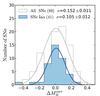 |
Fig. 12 SN Iaα corrected Hubble residual distributions
( |

SNe Iaα standardization generates a smooth symmetric residual distribution, with a significantly smaller magnitude dispersion of σ = 0.105 ± 0.012 mag (after 3σ clipping) than the full initial sample (σ = 0.152 ± 0.011 mag, no outlier). This dispersion agrees with the original M1 fit (0.099 ± 0.009 mag) and corresponds to a significant reduction of ~30% of the Hubble residual dispersion.
To check the robustness of this result we conducted several additional tests. First we considered the effect of including the 3σ outlier, SNF20070701-005. Doing so increases the residual standard deviation to 0.126 ± 0.014 mag (nMAD of 0.108 mag), but we note that this outlier falls within the brighter part of the distribution, potentially polluted by M2 SNe. This SN might just be a case of misassociation with a star-forming environment, as discussed in Sect. 3. This possibility is reinforced by the fact that this host is globally passive, with log (sSFR) = −10.8 (Childress et al. 2013a).
Next, we performed a permutation test based on independent standardization trials for 41 randomly selected SNe from the full sample. The results attest to the high significance of the environmental selection, giving p = 1.9 × 10⁻³.
Finally, K-fold cross-validation was employed to measure the predictive power of our model. Since it avoids overfitting the sample, cross-validation results are not expected to be as good as the original fit (Kim et al. 2013). We find σ = 0.117 ± 0.014 mag using k = 10, which is compatible with our original results. The quoted error includes a marginal dispersion of 0.004 mag from random “fold” selections.
6.3. Mitigation strategies
The Hα bias is a concern for cosmology, since it reveals a local environmental dependency, most probably a progenitor effect not accounted for by current SN standardization methods. It is necessary for ongoing and future surveys to consider it. The best solution would be if additional light curve or spectral features could be identified that can be used to remove the impact of local host properties. Another possibility would be to include the bimodality in the cosmology fitter, treating the redshift dependence and relative fraction of passive environments as free parameters. However, this seems perilous because it could mask or induce signatures of exotic dark energy, and would likely require light curves with much better statistical accuracy in order to resolve the bimodality. Implementation of our model from Sect. 6.1.1 also could be considered. Examining these and other model-dependent correction possibilities is left for future work. Alternatively, it could prove useful to focus on the Iaα subgroup for cosmological analyses, since these appear to be free of environmental biases.
For cosmological measurements naturally it is not permissible to split the SN Ia sample based solely on Hubble diagram residuals, e.g. one cannot directly select only the homogeneous Mode 1 SNe. However, one may select a subsample of SNe Ia based on their local environment properties: it is then possible to remove the brighter Mode 2, which is exclusively found in locally passive environments, by discarding the entire Iaϵ group. This is not as draconian as it may sound; while only ~50% of the sample would be retained, this subset has roughly 1.8 × as much statistical weight per SN. Thus, the statistical power is nearly the same as using the full sample. Of course obtaining local environment measurements could be observationally expensive, but Fig. 11 indicates that most of the bias is at lower redshifts, where local environment measurements are less difficult. Since Iaα appear to be dustier, this might add some complications, but in our dataset the Iaα standardize well despite this. We note that removing SNe from globally passive hosts will only remove approximately half of the SNe Iaϵ. However, at least then local measurements would not be needed for these.
In conclusion, SNe Ia from passive environments (Iaϵ) appear to cause the known (yet not understood) environmental biases, and we raise the possibility of removing them for cosmological studies. As SNe Iaα form an homogeneous subgroup of standardizable candles, free of environmental biases and therefore showing a tighter dispersion on the Hubble diagram, they could be used exclusively for cosmological analyses.
7. Robustness of the analysis
In this section, we analyze the robustness of our results, by testing potential issues in our analysis: (1) the impact of seeing given our 1 kpc aperture; (2) the influence of SNe potentially misassociated with Hα signal from host galaxy cores and (3) the influence of the ΣHα boundary defining the Iaϵ and Iaα subgroups. The general conclusion of these tests is that our results are not significantly affected by changes in our assumptions.
7.1. Restframe aperture and redshift bias
All our spectra have been averaged over an identical spatial aperture of 1 kpc radius (see Sect. 2.2.3). However, the atmospheric seeing PSF correlates spaxels on the arcsecond scale. For the SNfactory dataset the median seeing is 1''̣1. This corresponds to a projected correlation length of ~0.65 kpc at z = 0.03; ~1.1 kpc at z = 0.05, and ~1.6 kpc at z = 0.08. The redshift therefore has an influence on the amount of independent information in the 1 kpc radius aperture around the SN due to the seeing. Seeing also allows contamination of the local environment from bright sources outside the aperture.
However, a Spearman rank correlation analysis shows no correlation between log (ΣHα) and z (rs = 0.17, ps = 0.14), and both ΣHα subgroups have similar redshift distributions (pKS = 0.25). Consequently, we believe that our analysis is relatively unaffected by a redshift bias induced by seeing.
7.2. SNe with potentially misassociated Hα signals
Supernovae close to the center of very inclined hosts (referred to as “p.m.s”, see Sect. 3) have been directly removed from the main analysis, given the possible misassociation with Hα from the core of the galaxy. As described below, when we include those SNe, none of the previous results are significantly affected:
-
Color relation:
the observed correlation between c and ΣHα is slightly more significant, with a Spearman rank correlation coefficient of rs = 0.22 (ps = 0.035);
-
Hα bias:
the bias increases marginally, with
 mag,
(pKS = 6.5 × 10⁻³);
mag,
(pKS = 6.5 × 10⁻³); -
Stretch and host mass:
x1 and the total host stellar mass remain uncorrelated for SNe Iaα (rs = 0.07, ps = 0.66);
-
SNe Iaα dispersion:
the Iaα
dispersion increases to 0.115 ± 0.012 mag (p = 0.011), which is
still compatible with our fiducial result.
7.3. Influence of the Iaα/Iaϵ boundary
In our fiducial analysis the division between locally passive (Iaϵ) and locally star-forming (Iaα) subgroups was set at the median value log (ΣHα) = 38.35 of a 82 SN sample. The confidence interval for this population split is 37–45 (Cameron 2011). The numerical values for our main results when using this range for the Iaα/Iaϵ boundary are as follows:
-
Hα bias:
the biaschanges within the errors bars, with
 mag and
 mag for 37 and 45
Iaϵ, respectively;
mag for 37 and 45
Iaϵ, respectively; -
Stretch and host mass:
x1 and the total host stellar mass of the SNe Iaα remain uncorrelated in both cases, giving ps = 0.84;
-
SNe Iaα dispersion:
the Iaα
dispersion is the same within the error bars, with 0.115 ± 0.012 mag and
0.112 ± 0.012 mag for 37 and 45 Iaϵ, respectively.
The changes are minor, demonstrating the robustness of our analysis to a shift in the Iaα/Iaϵ limits.
Furthermore, in Sect. 3 we pointed out cases of SNe Iaϵ in globally star-forming hosts located near our division point, e.g., having log (ΣHα) ~ 38 and sSFR > −10. Whether they are truly locally passive or locally star-forming is therefore somewhat uncertain. As itemized below, we find that our main results do not depend on whether those SNe are included in the Iaα subgroup. However, three of these cases are bright and have been counted as M2 in our fiducial analysis, therefore moving them from Iaϵ to Iaα increases the dispersion of Hubble residuals of the SNe Iaα subset.
-
Hα bias:
the bias marginally changes, with
 mag;
mag; -
Stretch and host mass:
x1 and the total host stellar mass of the SNe Iaα remain uncorrelated, giving ps = 0.57;
-
SNe Iaα dispersion:
the Iaα
dispersion is degraded by the inclusion of bright SNe that skew the normal
distribution: σ = 0.144 ± 0.014 mag (no SNe have been clipped).
8. Summary and conclusion
Using the SuperNova Integral Field Spectrograph (SNIFS), we have assembled a sample of 89 nearby SNe Ia in the redshift range 0.03 < z < 0.08 with accurate measurements of the Hα surface brightness within a 1 kpc radius (ΣHα) used as a tracer of young stars in the SN neighborhood.
This sample was split in two at the median value log ΣHα = 38.35, which happens to correspond to the mean WIM Hα surface brightness of galaxies (Oey et al. 2007) and to the mean Hα sensitivity level at our highest redshift. SNe with low ΣHα were then designated as “locally passive” (Iaϵ), while those with high ΣHα were designated as “locally star-forming” (Iaα). The wide range of measured ΣHα indirectly confirms the existence of SNe Ia associated to both young and old stellar populations. We then studied variations in SNe properties as a function of this local host parameter as listed below.
Color:
our local analysis highlights a 2σ significance correlation between log (ΣHα) and the SALT2 color c, with the SNe Iaα being redder, as expected (Charlot & Fall 2000).
Stretch:
the relationship between SN light-curve stretch and local star formation activity is more complex than suggested by previous global host studies. Faster declining SNe (x1 < −1) are indeed strongly favored by locally passive environments, but passive local environments also host SNe with moderate stretches. Lower stretch SNe Ia are hosted in locally passive environments, but we find that moderate stretch SNe Ia are hosted by all types of environments. The local perspective also shows that the correlation between the host stellar mass and SN stretch is entirely created by the SNe Iaϵ. The stretches of SNe Iaα, from locally star-forming regions, are uncorrelated with the total stellar masses of their hosts.
Hubble residuals:
after routine SALT2 standardization using stretch and color, we showed that the SN Ia
Hubble residuals () are
significantly environment-dependent. SNe Iaϵ from locally passive regions
are 0.094 ± 0.031 mag brighter than SNe Iaα from locally star-forming
regions. This Hα bias stems from a bimodal structure in the Hubble
residual distribution. The first mode, denoted as M1, is
present in all environments, independent of the local star formation activity. The second
mode, M2, is intrinsically brighter, is exclusive to locally
passive environments, and occurs predominately in high-mass hosts. We noted that this
peculiar structure naturally explains the previously observed “mass step”, i.e. the offset
in brightness between SNe from low- and high-mass hosts (e.g., Childress et al. 2013a). This suggests that the Hα
bias is not exclusive to our sample and has a more fundamental origin than the global host
effect. Additional SN data, with measurement uncertainties below the 0.1 mag, will be
critical for confirming the Hubble residual bimodality. Our analysis does not suggest any
significant dependence on the local Hα environment of the stretch or
color coefficients used in standardization.
Cosmological implications:
the Hα bias is a concern for cosmology since the fraction of SNe in star-forming environments most likely changes with redshift, which implies an evolution with z of the mean B-magnitude of SNe Ia after standardization. Using a simple toy model based on the evolution of the specific star formation rate of galaxies with redshift, we estimated that this effect could shift the measurement of the dark energy equation of state parameter by Δw ~ −0.06. Currently employed constant mass-step corrections might accidently reduce or increase the bias on w, but not remove it. Moreover, the amplitude of the mass step is shown to evolve with redshift as predicted, which supports our claim that both the Hα bias and the mass step arise from the same underlying phenomenon. Future cosmological analyses will need to consider these environmental dependencies. An ideal solution would be to find additional light curve or spectral features able to correct this bias. Another solution would be to focus on a subsample of SNe Ia free from this known – yet not understood – biases.
SNe Iaα as homogeneous SALT2 candles:
SNe Ia from locally passive environments (Iaϵ) appear to be the cause of all the biases we have observed. We raised the idea of removing them from cosmological fits for this reason. The remaining bias-free SNe Iaα have an intrinsic Hubble residual dispersion reduced to 0.105 ± 0.012 mag, suggesting that a selection based on local environment would significantly improve the quality of SNe Ia as cosmological distance indicators. We further noted that this remaining dispersion is entirely consistent with our measurement uncertainties; no intrinsic dispersion is necessary. The cost of suppressing this serious bias would be a minor loss in net statistical power compared to using the full SN sample, and the need for measurements of the local environment.
At this juncture SN cosmology is limited by systematic errors (Conley et al. 2011; Saunders et al. 2013). Calibration issues are thought to set the current limits, but our first analysis of the local SN environments has revealed strong correlations between SNe and the star-forming activity of their immediate environment. This is most likely caused by our limited knowledge of the progenitors of the SNe Ia, the existence of potential SN subgroups, and the evolution with redshift of these standardizable candles.
For future SN cosmology efforts, we thus suggest further studies exploring the properties of SN Ia local host environments. Notably, the following local host properties may bring essential clues leading to the minimization of progenitor dependencies: gas and stellar metallicities, star formation history surrounding the SNe, and local interstellar dust extinction. Continuing to refine these measurements will constitute a major step forward in the direction of constructing an accurate “likes-to-likes” SN cosmology.
Online material
Appendix A: Relation between the Hα bias and the mass step
In this Appendix we provide the mathematical details needed to understand the relation between the ΣHα group magnitudes and the observed mass step. This derivation provides the relation between the numerical values of the Hα bias and the mass step in the SNfactory dataset.
To begin with, the dataset is partioned into four subsets consisting of SNe
Iaα and SNe Iaϵ above and below the canonical mass
division point of
log (M/M⊙) = 10. We
denote the number in each subset as Nα,L,
Nα,H,
Nϵ,L, and
Nϵ,H, with L and H symbolizing SNe Ia
in low- and high-mass hosts, respectively. Likewise, the mean Hubble residuals for each
subset are denoted as  ,
,
 ,
,
 , and
, and
 .
.
To make the equations more readable we introduce the following notation for fractions:
 means “the
fraction of SNe from subset A that have property B”.
For instance,
means “the
fraction of SNe from subset A that have property B”.
For instance,  means
“the fraction of SNe Ia from high-mass hosts that are Iaϵ”, i.e.,
Nϵ,H/NH.
Mathematically, B is the numerator and A the
denominator. Naturally, the partitioning imposes the requirement that
means
“the fraction of SNe Ia from high-mass hosts that are Iaϵ”, i.e.,
Nϵ,H/NH.
Mathematically, B is the numerator and A the
denominator. Naturally, the partitioning imposes the requirement that
 ,
e.g.,
,
e.g.,  .
.
Appendix A.1: General equations
The Hα bias,  , is defined as the
weighted mean difference of the
between the Iaϵ and Iaα subsamples:
, is defined as the
weighted mean difference of the
between the Iaϵ and Iaα subsamples:  (A.1)The mass step,
, is
defined as the weighted mean difference of the
between SNe Ia in low-mass and the high-mass hosts:
(A.1)The mass step,
, is
defined as the weighted mean difference of the
between SNe Ia in low-mass and the high-mass hosts:  (A.2)The individual
weighted mean magnitudes entering Eqs. (A.1) and (A.2) can be written
in terms of the weighted mean magnitudes for each portion. Introduction of our
notation
then gives
(A.2)The individual
weighted mean magnitudes entering Eqs. (A.1) and (A.2) can be written
in terms of the weighted mean magnitudes for each portion. Introduction of our
notation
then gives  Combining
these we obtain the equations for the Hα bias and mass step in terms
of the partitioned data:
Combining
these we obtain the equations for the Hα bias and mass step in terms
of the partitioned data:  With
this development it is now possible to write the mass step directly in terms of the
Hα bias, as follows:
With
this development it is now possible to write the mass step directly in terms of the
Hα bias, as follows:  (A.9)In
this expression we have simply rearranged terms to demonstrate that the same weighted
mean magnitudes, just having different signs and fractions, appear in both the
numerator and denominator.
(A.9)In
this expression we have simply rearranged terms to demonstrate that the same weighted
mean magnitudes, just having different signs and fractions, appear in both the
numerator and denominator.
Appendix A.2: Observational constraints
Equation (A.9) is exact when all of
the quantities can be directly measured, as they are in our dataset. These variables
can be generalized to any similar dataset. In order to be exact, though, observations
of the local environment would be required. However, in the main text we presented two
observational constraints that can be used to greatly simply Eq. (A.9). First, we have shown in Sect. 5.2.2 that the averaged
of SNe
Iaα does not depend on the masses of their hosts:  (A.10)Second, we observed
in Fig. 10 that SNe Iaα and
Iaϵ from low-mass hosts share the same mean magnitude (within error
bars):
(A.10)Second, we observed
in Fig. 10 that SNe Iaα and
Iaϵ from low-mass hosts share the same mean magnitude (within error
bars):  (A.11)As a consequence of
these two observations, the righthand side of Eq. (A.7) becomes
(A.11)As a consequence of
these two observations, the righthand side of Eq. (A.7) becomes  (A.12)Similarly,
the righthand side of Eq. (A.8)
becomes
(A.12)Similarly,
the righthand side of Eq. (A.8)
becomes  (A.13)Finally,
using the relation
(A.13)Finally,
using the relation  , where
Fϵ is the fraction of SNe
Iaϵ, and FH the fraction of SNe Ia from
high-mass hosts, Eq. (A.9) can simply
be expressed as
, where
Fϵ is the fraction of SNe
Iaϵ, and FH the fraction of SNe Ia from
high-mass hosts, Eq. (A.9) can simply
be expressed as  (A.14)In the main
text, the dependence of Fϵ with redshift
is denoted ψ(z), and
is assumed to be
constant. Furthermore, based on the dataset we compiled in Childress et al. (2013a), FH appears to
be constant within 10% up to z ~ 1. Subject to these approximations,
we conclude that the mass-step evolution is simply proportional to
ψ(z), as given in Eq. (6).
(A.14)In the main
text, the dependence of Fϵ with redshift
is denoted ψ(z), and
is assumed to be
constant. Furthermore, based on the dataset we compiled in Childress et al. (2013a), FH appears to
be constant within 10% up to z ~ 1. Subject to these approximations,
we conclude that the mass-step evolution is simply proportional to
ψ(z), as given in Eq. (6).
See Childress et al. (2013b) for details on the measurement of sSFR for the SNfactory sample.
Acknowledgments
We thank Dan Birchall for observing assistance, the technical and scientific staffs of the Palomar Observatory, the High Performance Wireless Radio Network (HPWREN), and the University of Hawaii 2.2 m telescope. We recognize the significant cultural role of Mauna Kea within the indigenous Hawaiian community, and we appreciate the opportunity to conduct observations from this revered site. This research was conducted within the framework of the Lyon Institute of Origins under grant ANR-10-LABX-66. M.R. thanks French Rhône-Alpes region for support from its grant Explo’ra doc 11-015443-03. This work was supported by the Director, Office of Science, Office of High Energy Physics, of the US Department of Energy under Contract No. DE-AC02-05CH11231; by a grant from the Gordon & Betty Moore Foundation; in France by support from CNRS/IN2P3, CNRS/INSU, and PNCG; and in Germany by the DFG through TRR33 “The Dark Universe”. Some results were obtained using resources and support from the National Energy Research Scientific Computing Center, supported by the Director, Office of Science, Office of Advanced Scientific Computing Research, of the US Department of Energy under Contract No. DE-AC02-05CH11231. HPWREN is funded by National Science Foundation Grant Number ANI-0087344, and the University of California, San Diego. Based in part on observations made with the NASA Galaxy Evolution Explorer, operated for NASA by the California Institute of Technology under NASA contract NAS5-98034, with analysis supported by GALEX Archival Research Grant #08-GALEX508-0008 for program GI5-047 (PI: Aldering).
References
- Aihara, H., Allen de Prieto, C., An, D., et al. 2011, ApJS, 193, 29 [NASA ADS] [CrossRef] [Google Scholar]
- Aldering, G., Adam, G., Antilogus, P., et al. 2002, in Survey and Other Telescope Technologies and Discoveries, Proc. SPIE, 4836, 61 [Google Scholar]
- Aldering, G., Antilogus, P., Bailey, S., et al. 2006, ApJ, 650, 510 [NASA ADS] [CrossRef] [Google Scholar]
- Alvarez, M. A., Bromm, V., & Shapiro, P. R. 2006, ApJ, 639, 621 [NASA ADS] [CrossRef] [Google Scholar]
- Amanullah, R., Lidman, C., Rubin, D., et al. 2010, ApJ, 716, 712 [NASA ADS] [CrossRef] [Google Scholar]
- Aubourg, E., Tojeiro, R., Jimenez, R., et al. 2008, A&A, 492, 631 [NASA ADS] [CrossRef] [EDP Sciences] [Google Scholar]
- Bailey, S., Aldering, G., Antilogus, P., et al. 2009, A&A, 500, L17 [NASA ADS] [CrossRef] [EDP Sciences] [Google Scholar]
- Bartunov, O. S., Tsvetkov, D. Y., & Filimonova, I. V. 1994, PASP, 106, 1276 [NASA ADS] [CrossRef] [Google Scholar]
- Bongard, S., Soulez, F., Thiébaut, E., & Pecontal, E. 2011, MNRAS, 418, 258 [NASA ADS] [CrossRef] [Google Scholar]
- Burnham, K. P., & Anderson, D. R. 2002, Model Selection and Multi-Model Inference: A Practical Information-Theoretic Approach (Springer) [Google Scholar]
- Buton, C., Copin, Y., Aldering, G., et al. 2013, A&A, 549, 8 [NASA ADS] [Google Scholar]
- Calzetti, D. 2012 [arXiv:1208.2997] [Google Scholar]
- Calzetti, D., Kinney, A. L., & Storchi-Bergmann, T. 1994, ApJ, 429, 582 [NASA ADS] [CrossRef] [Google Scholar]
- Calzetti, D., Wu, S.-Y., Hong, S., et al. 2010, ApJ, 714, 1256 [NASA ADS] [CrossRef] [Google Scholar]
- Cameron, E. 2011, PASA, 28, 128 [NASA ADS] [CrossRef] [Google Scholar]
- Charlot, S., & Fall, S. M. 2000, ApJ, 539, 718 [NASA ADS] [CrossRef] [Google Scholar]
- Childress, M., Aldering, G., Antilogus, P., et al. 2013a, ApJ, 770, 108 [NASA ADS] [CrossRef] [Google Scholar]
- Childress, M., Aldering, G., Antilogus, P., et al. 2013b, ApJ, 770, 107 [NASA ADS] [CrossRef] [Google Scholar]
- Chotard, N., Gangler, E., Aldering, G., et al. 2011, A&A, 529, L4 [NASA ADS] [CrossRef] [EDP Sciences] [Google Scholar]
- Conley, A., Guy, J., Sullivan, M., et al. 2011, ApJS, 192, 1 [NASA ADS] [CrossRef] [EDP Sciences] [Google Scholar]
- Damen, M., Labbé, I., Franx, M., et al. 2009, ApJ, 690, 937 [NASA ADS] [CrossRef] [Google Scholar]
- D’Andrea, C. B., Gupta, R. R., Sako, M., et al. 2011, ApJ, 743, 172 [NASA ADS] [CrossRef] [Google Scholar]
- de Zeeuw, P. T., Hoogerwerf, R., de Bruijne, J. H. J., Brown, A. G. A., & Blaauw, A. 1999, AJ, 117, 354 [NASA ADS] [CrossRef] [Google Scholar]
- Gallazzi, A., Charlot, S., Brinchmann, J., White, S. D. M., & Tremonti, C. A. 2005, MNRAS, 362, 41 [NASA ADS] [CrossRef] [Google Scholar]
- Girardi, L., Bressan, A., Bertelli, G., & Chiosi, C. 2000, A&AS, 141, 371 [NASA ADS] [CrossRef] [EDP Sciences] [Google Scholar]
- Groves, B., Brinchmann, J., & Walcher, C. J. 2012, MNRAS, 419, 1402 [NASA ADS] [CrossRef] [Google Scholar]
- Gupta, R. R., D’Andrea, C. B., Sako, M., et al. 2011, ApJ, 740, 92 [NASA ADS] [CrossRef] [Google Scholar]
- Guy, J., Astier, P., Baumont, S., et al. 2007, A&A, 466, 11 [NASA ADS] [CrossRef] [EDP Sciences] [Google Scholar]
- Guy, J., Sullivan, M., Conley, A., et al. 2010, A&A, 523, 7 [Google Scholar]
- Hamuy, M., Trager, S. C., Pinto, P. A., et al. 2000, AJ, 120, 1479 [NASA ADS] [CrossRef] [Google Scholar]
- Hanuschik, R. W. 2003, A&A, 407, 1157 [NASA ADS] [CrossRef] [EDP Sciences] [Google Scholar]
- Hopkins, A. M., & Beacom, J. F. 2006, ApJ, 651, 142 [NASA ADS] [CrossRef] [MathSciNet] [Google Scholar]
- James, P. A., & Anderson, J. P. 2006, A&A, 453, 57 [NASA ADS] [CrossRef] [EDP Sciences] [Google Scholar]
- Jha, S., Riess, A. G., & Kirshner, R. P. 2007, AJ, 659, 122 [Google Scholar]
- Johansson, J., Thomas, D., Pforr, J., et al. 2013, MNRAS, 435, 1680 [NASA ADS] [CrossRef] [Google Scholar]
- Kauffmann, G., Heckman, T. M., White, S. D. M., et al. 2003, MNRAS, 341, 54 [Google Scholar]
- Kelly, P. L., Hicken, M., Burke, D. L., Mandel, K. S., & Kirshner, R. P. 2010, ApJ, 715, 743 [NASA ADS] [CrossRef] [Google Scholar]
- Kennicutt, R. C. 1998, ARA&A, 36, 189 [Google Scholar]
- Kennicutt, R. C., & Evans, N. J. 2012, ARA&A, 50, 531 [NASA ADS] [CrossRef] [Google Scholar]
- Kim, A. G., Thomas, R. C., Aldering, G., et al. 2013, ApJ, 766, 84 [NASA ADS] [CrossRef] [Google Scholar]
- Koleva, M., Prugniel, P., Ocvirk, P., Le Borgne, D., & Soubiran, C. 2008, MNRAS, 385, 1998 [NASA ADS] [CrossRef] [Google Scholar]
- Koleva, M., Prugniel, P., Bouchard, A., & Wu, Y. 2009, A&A, 501, 1269 [NASA ADS] [CrossRef] [EDP Sciences] [Google Scholar]
- Konishi, K., Cinabro, D., Garnavich, P. M., et al. 2011 [arXiv:1101.4269] [Google Scholar]
- Kowalski, M., Rubin, D., Aldering, G., et al. 2008, ApJ, 686, 749 [NASA ADS] [CrossRef] [Google Scholar]
- Lampeitl, H., Smith, M., Nichol, R. C., et al. 2010, ApJ, 722, 566 [NASA ADS] [CrossRef] [Google Scholar]
- Lantz, B., Aldering, G., Antilogus, P., et al. 2004, in Optical Design and Engineering, Proc. SPIE, 5249, 146 [Google Scholar]
- Lee, J. H., Hwang, N., & Lee, M. G. 2011, ApJ, 735, 75 [NASA ADS] [CrossRef] [Google Scholar]
- Mannucci, F., Della Valle, M., Panagia, N., et al. 2005, A&A, 433, 807 [NASA ADS] [CrossRef] [EDP Sciences] [Google Scholar]
- Mannucci, F., Della Valle, M., & Panagia, N. 2006, MNRAS, 370, 773 [NASA ADS] [CrossRef] [Google Scholar]
- Maoz, D., & Mannucci, F. 2012, PASA, 29, 447 [NASA ADS] [CrossRef] [Google Scholar]
- Neill, J. D., Sullivan, M., Howell, D. A., et al. 2009, ApJ, 707, 1449 [NASA ADS] [CrossRef] [Google Scholar]
- Oey, M. S., Meurer, G. R., Yelda, S., et al. 2007, ApJ, 661, 801 [NASA ADS] [CrossRef] [Google Scholar]
- Paladini, R., Davies, R. D., & De Zotti, G. 2004, MNRAS, 347, 237 [NASA ADS] [CrossRef] [Google Scholar]
- Pereira, R., Thomas, R. C., Aldering, G., et al. 2013, A&A, 554, 27 [Google Scholar]
- Perlmutter, S., Aldering, G., Goldhaber, G., et al. 1999, ApJ, 517, 565 [NASA ADS] [CrossRef] [Google Scholar]
- Phillips, M. M. 1993, ApJ, 413, L105 [NASA ADS] [CrossRef] [Google Scholar]
- Portegies Zwart, S. F., McMillan, S. L. W., & Gieles, M. 2010, ARA&A, 48, 431 [NASA ADS] [CrossRef] [Google Scholar]
- Pérez-González, P. G., Rieke, G. H., Villar, V., et al. 2008, ApJ, 675, 234 [NASA ADS] [CrossRef] [Google Scholar]
- Riess, A. G., Press, W. H., & Kirshner, R. P. 1996, ApJ, 473, 88 [NASA ADS] [CrossRef] [Google Scholar]
- Riess, A. G., Filippenko, A. V., Challis, P., et al. 1998, AJ, 116, 1009 [NASA ADS] [CrossRef] [Google Scholar]
- Röser, S., Kharchenko, N. V., Piskunov, A. E., et al. 2010, Astron. Nachr., 331, 519 [NASA ADS] [CrossRef] [Google Scholar]
- Sánchez-Blázquez, P., Peletier, R. F., Jiménez-Vicente, J., et al. 2006, MNRAS, 371, 703 [NASA ADS] [CrossRef] [Google Scholar]
- Saunders, C., Aldering, G., Aragon, C., et al. 2013 [Google Scholar]
- Scalzo, R. A., Aldering, G., Antilogus, P., et al. 2010, ApJ, 713, 1073 [NASA ADS] [CrossRef] [Google Scholar]
- Scannapieco, E., & Bildsten, L. 2005, ApJ, 629, L85 [NASA ADS] [CrossRef] [Google Scholar]
- Schlegel, D. J., Finkbeiner, D. P., & Davis, M. 1998, ApJ, 500, 525 [NASA ADS] [CrossRef] [Google Scholar]
- Seon, K.-I., & Witt, A. N. 2012, ApJ, 758, 109 [NASA ADS] [CrossRef] [Google Scholar]
- Stanishev, V., Rodrigues, M., Mourão, A., & Flores, H. 2012, A&A, 545, 58 [Google Scholar]
- Sullivan, M., Le Borgne, D., Pritchet, C. J., et al. 2006, ApJ, 648, 868 [NASA ADS] [CrossRef] [Google Scholar]
- Sullivan, M., Conley, A., Howell, D. A., et al. 2010, MNRAS, 406, 782 [NASA ADS] [Google Scholar]
- Suzuki, N., Rubin, D., Lidman, C., et al. 2012, ApJ, 746, 85 [NASA ADS] [CrossRef] [Google Scholar]
- Tremonti, C. A., Heckman, T. M., Kauffmann, G., et al. 2004, ApJ, 613, 898 [NASA ADS] [CrossRef] [Google Scholar]
- Tripp, R. 1998, A&A, 331, 815 [NASA ADS] [Google Scholar]
All Tables
Definition of the two ΣHα subgroups, and their respective weighted mean light-curve parameters.
All Figures
|
Fig. 1 Top and bottom: the hosts of SN 2007kk (UGC 2828) and SN 2005L (MCG+07-33-005), respectively, both classified as globally star-forming (Childress et al. 2013b). Left: color images made using observations from SNIFS and SDSS-III (Aihara et al. 2011). On both images, the field-of-view of SNIFS, centered on the SN position (white-star marker), is indicated by the orange central square. Right: Hα surface brightness maps of the SN vicinities (the generation of these maps is detailed in Sect. 2.3). SN 2007kk occurred in a passive environment more than 1.5 kpc from the closest star-forming region, while SN 2005L is located at the edge of such a region. |
| In the text | |
|
Fig. 2 SN subtraction from a host cube. Different reconstructed images, made by integrating x,y,λ cubes along the λ axis, are shown for a single observation of SNF20070326-012. Top left: original flux-calibrated cube containing host, sky, and SN signals. Bottom left: pure SN cube obtained after host subtraction (image) and fitted PSF model (contours). Right: SN-subtracted host cube. |
| In the text | |
|
Fig. 3 Sky subtraction process for an R cube of host-SNF20060512-001. Top right: reconstructed image of a final reference acquisition (it could as well be an SN-subtracted cube); the central star marker indicates the SN location. The dot markers indicate the faintest spaxels used to measure the presumed sky. Top left: modeled sky (thick black) fit over the mean of the five faintest spectra (thin colored); the bottom part shows the fit residuals, compared to the presumed sky error (blue band). Bottom: host spectrum at the SN location before (upper thin gray line) and after (lower thick red line) the sky subtraction. The emission at 6830 Å is the Hα+[N ii] gas line complex, left untouched by the sky subtraction procedure. The few small features further toward the red are residuals from the sky subtraction, but this part of the spectrum is not used in this analysis. See Sect. 2.3 for details. |
| In the text | |
|
Fig. 4 Spectral fit of the host mean spectrum in the projected 1 kpc radius around SNF20060512-001. Top right: reconstructed image of a final reference exposure. The circle aperture shows the 1 kpc aperture centered on the SN location (central star marker). Top left: mean host spectrum within 1 kpc radius around the SN (rest-frame, green dashed-line with ± 1σ error band), averaged over 21 cubes (including two final references). The best ULySS fit is shown as the sum of a stellar continuum (red line) and gas lines (magenta dashed line). Bottom, from left to right: zoom on [O ii]λλ3726,3728, 4000 Å break, and Hα + [N ii]λλ6548,6584 + [S ii]λλ6716,6731 wavelength regions. |
| In the text | |
|
Fig. 5 Local vs. global star-forming environment. Blue squares and open-circles show the SNe Ia from locally star-forming and passive regions, respectively (log (ΣHα) ≷ 38.35, blue-dotted line). Gray arrows indicate points with ΣHα signals compatible with zero (detection at less than 2σ). The red-dashed line indicates the limit that is commonly used to distinguish between star-forming and passive galaxies when using global host galaxy measurements (log (sSFR) ≷ −10.5). Three SNe Ia from our sample do not have sSFR measurements. |
| In the text | |
|
Fig. 6 SN Ia parameters as a function of log (ΣHα), the surface
brightness in the 1 kpc radius around the SNe Ia. Upper panel: the
log (ΣHα) distribution colored with respect to
ΣHα subgroups: Iaϵ and
Iaα are shown as empty-black and filled-blue histograms,
respectively. Main panels, from top to bottom: SALT2 stretch
x1, color c, and the Hubble residuals
corrected for stretch and color |
| In the text | |
|
Fig. 7 SALT2 stretch x1 vs. color c. Left: the local perspective. SNe markers and x1 and c marginalized stacked distributions follow the same color-shape code as Fig. 6. Right: the global perspective. Open-blue squares show the globally star-forming hosts and red dots show the globally passive hosts (log (sSFR) ≶ −10.5 respectively). Big markers indicate SNe with local measurements, while small markers denote SNe not in our local sample (failed redshift cut, but passed the quality cuts, see Sect. 2.1). Stacked histograms are the marginalized distributions of x1 and c using the marker color codes. These figures compare to Fig. 2 of Lampeitl et al. (2010). Notice the mix of local environments for moderate x1 while low x1 are almost exclusively from passive environments. |
| In the text | |
|
Fig. 8 Distribution of corrected Hubble residuals per ΣHα
group (top, as in Fig. 6)
and per mode (bottom) for the full sample. In the lower panel,
the open-red and the filled-gray histograms represent the corrected Hubble
residual distributions of M1 and
M2, respectively. By definition of the modes, the
red histogram corresponds to the stack of the blue distribution with the open
histogram above |
| In the text | |
|
Fig. 9 SN Ia x1 vs. total host stellar mass (Childress et al. 2013a). Markers follow the same color and shape code as in Fig. 6. Note the distinctive “L”-shaped distribution of the SNe Iaϵ. |
| In the text | |
|
Fig. 10 Corrected Hubble residuals as a function of the total host stellar mass, showing
the mass step. Markers follow the same color and shape code as in Fig. 6. Top: total host stellar mass
distribution per ΣHα subgroup. Right:
|
| In the text | |
|
Fig. 11 Observed and predicted redshift evolution of the
|
| In the text | |
|
Fig. 12 SN Iaα corrected Hubble residual distributions
( |
| In the text | |
Current usage metrics show cumulative count of Article Views (full-text article views including HTML views, PDF and ePub downloads, according to the available data) and Abstracts Views on Vision4Press platform.
Data correspond to usage on the plateform after 2015. The current usage metrics is available 48-96 hours after online publication and is updated daily on week days.
Initial download of the metrics may take a while.