| Issue |
A&A
Volume 556, August 2013
|
|
|---|---|---|
| Article Number | A63 | |
| Number of page(s) | 18 | |
| Section | Interstellar and circumstellar matter | |
| DOI | https://doi.org/10.1051/0004-6361/201220910 | |
| Published online | 29 July 2013 | |
The degeneracy between dust colour temperature and spectral index
Comparison of methods for estimating the β(T) relation
1
Department of Physics, PO Box 64, 00014 University of Helsinki,
Finland
e-mail:
This email address is being protected from spambots. You need JavaScript enabled to view it.
2
Institut dAstrophysique Spatiale, UMR 8617, CNRS/Université
Paris-Sud 11, 91405
Orsay,
France
Received:
13
December
2012
Accepted:
27
May
2013
Abstract
Context. Submillimetre dust emission provides information on the physics of interstellar clouds and dust. However, noise can produce a spurious anticorrelation between the colour temperature TC and the spectral index β. These artefacts must be separated from the intrinsic β(T) relation of dust emission.
Aims. We compare methods that can be used to analyse the β(T) relation. We wish to quantify their accuracy and bias, especially for observations similar to those made with Planck and Herschel.
Methods. We examine submillimetre observations that are simulated either as simple, modified black body emission or using 3D radiative transfer modelling. We used different methods to recover the (T, β) values of individual objects and the parameters of the β(T) relation. In addition to χ2 fitting, we examined the results of the SIMEX method, basic Bayesian model, hierarchical models, and a method that explicitly assumes a functional form for β(T). The methods were also applied to one field observed by Herschel.
Results. All methods exhibit some bias, even in the idealised case of white noise. The results of the Bayesian method show significantly lower bias than direct χ2 fits. The same is true for hierarchical models that also result in a smaller scatter in the temperature and spectral index values. However, significant bias was observed in cases with high noise levels. When the signal-to-noise ratios are different for different sources, all β and T estimates of the hierarchical model are biased towards the relation determined by the data with the highest signal-to-noise ratio. This can significantly alter the recovered β(T) function. With the method where we explicitly assume a functional form for the β(T) relation, the bias is similar to the Bayesian method. In the case of the actual Herschel field, all methods agree on some degree of anticorrelation between T and β.
Conclusions. The Bayesian method and the hierarchical models can both reduce the noise-induced parameter correlations. However, all methods can exhibit non-negligible bias. This is particularly true for hierarchical models and observations of varying signal-to-noise ratios and this must be taken into account when interpreting the results.
Key words: ISM: clouds / infrared: ISM / radiative transfer / submillimeter: ISM
© ESO, 2013
1. Introduction
Observations of submillimetre and millimetre dust emission are considered one of the most reliable ways of mapping dense clouds and cloud cores in different phases of the star formation process (Motte et al. 1998; André et al. 2000; Enoch et al. 2007; André et al. 2010). Many other tracers suffer from some serious problems, especially in the case of dense prestellar and protostellar cores. The interpretation of molecular line data is complicated by the abundance variations and the optical depth effects and very high-resolution maps of dust extinction and scattering are difficult to obtain (Lombardi et al. 2006; Goodman et al. 2009; Juvela et al. 2008, 2009).
In addition to being a tracer of the structure of interstellar clouds, the dust emission carries information on the properties of the dust grains themselves. These are expected to vary from region to region. The grain optical properties depend on their chemical composition, and the dust size distribution is modified by the competing effects of dust erosion (e.g., by shock waves) and aggregation processes (e.g., Ormel et al. 2011; Jones & Nuth 2011). The grain emissivity may even depend on the temperature of the grains but is certainly modified by the ice mantles that are acquired in cold cloud cores (Ossenkopf & Henning 1994; Stepnik et al. 2003; Meny et al. 2007; Compiègne et al. 2011). Because these changes depend on the local current and past conditions, they could, in principle, be used to trace the physical evolution of the clouds and their dust during the star formation process. Thus, accurate measurements of the dust properties would be very valuable.
Unfortunately, it is difficult to deduce intrinsic dust properties based on the observed radiation. Some of the difficulties are caused by the line-of-sight temperature variations that broaden the emission spectrum, decreasing the observed spectral index β (Shetty et al. 2009b; Malinen et al. 2011; Juvela & Ysard 2012b). At the same time, the dust colour temperature TC overestimates the mass averaged physical dust temperature, and the total dust mass becomes underestimated (Evans et al. 2001; Stamatellos & Whitworth 2003; Malinen et al. 2011; Ysard et al. 2012). If the exact nature of the line-of-sight temperature variations is not known, it is difficult to accurately measure the intrinsic dust emissivity spectral index.
We want to know to what accuracy the basic parameters of dust temperature and dust emissivity spectral index can be deduced from observations. In the present paper, we concentrate on the complications caused by the noise present in the measured submillimetre intensity values. When dust observations are fitted with modified black body spectra, the dust colour temperature, TC, and the observed dust spectral index, β, are partly degenerate. The noise will scatter the observed TC and β values over an elongated ellipse that shows apparent negative correlation between the parameters. In the limit of low noise, the errors are correlated, but the expectation values are not significantly biased. If the noise is greater, error regions become banana-shaped because the β(TC) relation gets steeper at lower temperatures (Shetty et al. 2009b,a; Veneziani et al. 2010; Paradis et al. 2010; Juvela et al. 2011). The parameter distributions can become skewed, and in rare cases, the χ2 values of the modified black body fits may even have separate minima that are several degrees apart in TC (Juvela & Ysard 2012a). Under these conditions, the (TC, β) values determined for individual sources (or for pixels in a map) are not only uncertain but also biased.
The β(TC) relation induced by the noise is usually steeper than the average β(TC) relation derived from observations of a set of sources (Dupac et al. 2003; Désert et al. 2008; Planck Collaboration 2011). Therefore, the noise tends to make the estimated β(TC) relation steeper than the true relation. The bias can be significant even at noise levels below 10%. With perfect knowledge of the observational noise, one should be able to eliminate these effects and to recover the unbiased (TC, β) estimates for the sources and to determine the true overall β(TC) relation. Even this would be the true relation only in the sense that it would accurately describe the observed radiation. It would still not describe the intrinsic grain properties because of line-of-sight temperature variations within the source and, in extreme cases, by opacity effects.
The effect of the noise can be tackled in different ways. In the Bayesian formulation one probes the posterior probability P(θ|d) ∝ P(θ)P(d|θ), where P(θ) is the a priori probability of the parameters θ and P(d|θ) the likelihood function. The probability P(θ|d) can be estimated with Markov chain Monte Carlo (MCMC) calculations (e.g. Veneziani et al. 2010) to recover less biased β and T estimates. In the hierarchical Bayesian method, one additionally includes a global model for the distribution of the T and β (and column density) values (Kelly et al. 2012). If one is mainly interested in the overall relation β(TC), one also can start with the observed values and employ direct Monte Carlo simulation to estimate how much the estimated β(T) relation is affected by the assumed level of noise (Planck Collaboration 2011). The procedure also can be automatised, looking for a β(T) relation that corresponds to the observations when the effect of the noise, estimated with Monte Carlo methods, is added. On the other hand, SIMEX (Cook & Stefanski 1994) is a very general method where the results are examined as a function of the input noise and the final de-biased estimate is obtained by an extrapolation to zero noise level. In this paper we compare the methods listed above, also including some variations of the hierarchical models. Our main goal is to quantify the accuracy by which the β(TC) relation can be derived, for example, from observations carried out by Planck (Tauber et al. 2010) and Herschel1 (Pilbratt et al. 2010). This particularly includes the examination of the bias.
The content of the paper is the following. In Sect. 2 we present the methods that are used to analyse intensity measurements and to derive the parameters of β(TC) relation. Section 3 describes the data used in the tests. These include simple modified black body spectra (Sect. 3.1), surface brightness maps obtained with radiative transfer modelling (Sect. 3.2), and actual Herschel data (Sect. 3.3). The corresponding results are presented in Sects. 4–6. The results are discussed in Sect. 7 and the final conclusions are listed in Sect. 8.
2. Analysis methods
In this section we present the methods that are used to estimate the (T, β) values of individual sources and the parameters (A, B) of the β(T) relation (see Eq. (10)) for a collection of sources.
2.1. The χ2 fitting
The derivation of the modified black body parameters and of the β(T) relation is often based on direct maximum likelihood estimates. Apart from possible filtering of outliers and other allowances for deviations from the normal statistics, the least squares fitting still remains the basic method. The analysis is performed in two stages. The (T, β) values are first estimated for each source (or pixel) separately, fitting the intensities at the observed wavelengths with a modified black body law, using weighted least squares. The estimated (T, β) points are then fitted with a parametric curve that, in our case, is Eq. (10) with the parameters A and B.
We call the above the χ2 method because both steps steps can be based on χ2 minimisation. The uncertainties δT and δβ can be estimated based on the measurement errors using, for example, Monte Carlo methods. When the analytical β(T) relation is fitted, the uncertainties of the individual intensity measurements are no longer considered, and one only relies on the previously derived δT and δβ estimates. We explicitly ignore the information on the correlations of the T and β errors.
2.2. SIMEX method
In the SIMEX method (Cook & Stefanski 1994), one examines how the results change as a function of the noise. The final result is obtained by extrapolating this relation to a zero noise level. Because the (T, β) measurements of individual sources usually do not exhibit clear bias, SIMEX is not useful in their analysis. Only when the signal-to-noise ratio is very low can the error distributions of say the spectral index become skew (Juvela & Ysard 2012a), and SIMEX could be used to quantify the effect. In this paper, we only examine SIMEX estimates of the A and B parameters of the β(T) relation.
In each case, we generate 1000 noise realisations where the noise level is varied from that of the actual observation to a case with three times the original noise. We add Gaussian noise to the intensity measurements (that already contain the original observational noise), perform the modified black body fits for all sources, and fit the β(T) relation with the least squares method. This gives us 1000 points describing the change in the parameters A and B as functions of the noise. We perform linear fits to these relations, and the extrapolation to zero noise level gives the bias-corrected estimates of A and B.
The use of the SIMEX method requires reliable estimates of the noise level of the data. Because of the extrapolation, the statistical noise will be enhanced, but if the noise dependence is well defined, SIMEX could reduce the bias. There is no guarantee that the functional form of the noise dependence is similar at low and high noise levels. The result will depend on the range of noise levels examined and on the functional form used for the fitting and extrapolation. If the extrapolation function is not adequate for the problem at hand, the method could even increase the bias.
2.3. Bayesian method
In the Bayesian method one estimates the posterior probability
p(θ|d) of model parameters
θ for given data d. It presents the advantage of
giving the parameters that maximise
p(θ|d) and, at the same time,
providing error estimates via their probability distribution. Using Bayes formula, the
posterior probability of model parameters for given data,
p(θ|d) can be written as
 (1)Here
p(θ) is the prior probability assigned to the
parameters θ and the last term,
p(d|θ), is called the likelihood
function that gives the probability of data d for a given set of model
parameters θ. The parameter vector θ contains estimates
for the intensity (or flux), temperature, and spectral index of each source. In our case
p(d|θ) corresponds to the combined
probability of the fits of modified black body spectra to the observations of individual
sources. We assume a flat prior. Thus, the probability can be calculated based on the
combined χ2 value of those fits, assuming normal statistics
(1)Here
p(θ) is the prior probability assigned to the
parameters θ and the last term,
p(d|θ), is called the likelihood
function that gives the probability of data d for a given set of model
parameters θ. The parameter vector θ contains estimates
for the intensity (or flux), temperature, and spectral index of each source. In our case
p(d|θ) corresponds to the combined
probability of the fits of modified black body spectra to the observations of individual
sources. We assume a flat prior. Thus, the probability can be calculated based on the
combined χ2 value of those fits, assuming normal statistics
![Mathematical equation: \begin{equation} \ln p(d|\theta) \propto \sum_{i=1}^{N_{\rm S}} \sum_{j=1}^{N_{\rm f}} \left[ \frac{S_{i,j}-S_{\rm model}}{{\rm d}S_{i, j}}, \right]^2 \end{equation}](/articles/aa/full_html/2013/08/aa20910-12/aa20910-12-eq23.png) (2)where
the sum includes flux measurements S and their error estimates
dS for all the NS sources and
Nf frequencies. We evaluate
p(θ|d) using MCMC. In the
Metropolis-Hastings algorithm, one generates parameter steps
θi → θi + 1, using some
propositional probability distribution for the step. The step is then accepted if
(2)where
the sum includes flux measurements S and their error estimates
dS for all the NS sources and
Nf frequencies. We evaluate
p(θ|d) using MCMC. In the
Metropolis-Hastings algorithm, one generates parameter steps
θi → θi + 1, using some
propositional probability distribution for the step. The step is then accepted if
 (3)where
u is a uniformly distributed random number between 0 and 1. Thus, the
calculation only requires knowing the ratio of the probabilities. The accepted
θi values sample the posterior probability distribution
p(θ|d) (see, e.g., Veneziani et al. 2010).
(3)where
u is a uniformly distributed random number between 0 and 1. Thus, the
calculation only requires knowing the ratio of the probabilities. The accepted
θi values sample the posterior probability distribution
p(θ|d) (see, e.g., Veneziani et al. 2010).
We generate the parameter steps using normal distribution. The relative step sizes of the different parameters are fixed beforehand but the absolute step length is adjusted with a single multiplicative factor to keep the acceptance rate close to 20%. After the initial burn-in phase, MCMC samples the posterior probability distribution Eq. (1) and, using values from a long enough piece of the chain, one can directly estimate the distributions of the parameters. We run the MCMC in pieces of about million steps. The parameter distributions in each piece of the chain are examined to make sure that a convergence was reached. The reported results are calculated from the last part of the chain.
It would be possible to extract samples from the MCMC parameter distributions to also estimate distributions for the parameters A and B of the β(T) relation. However, we fit the β(T) relation to the average T and β values obtained for each individual source. This allows direct comparison with other methods (e.g., χ2 and SIMEX).
2.4. Bayesian hierarchical model
In the Bayesian hierarchical model, one combines the models of the individual sources with a global model that describes the overall distribution of source parameters (Kelly et al. 2012). In our case, the basic source parameters are the intensity Ii at a reference wavelength, the temperature Ti, and the spectral index βi. When analysing maps, each pixel is considered as a separate source.
The posterior probability is calculated from ![Mathematical equation: \begin{equation} p(I, T, \beta, \delta | S) \propto p(\theta) \prod_{i=1}^{N_{\rm S}} \left[ p(I_i, T_i, \beta_i|\theta) \prod_{j=1}^{N_{\rm f}} p(S_{i,j}| I_i, T_i, \beta_i, \delta_j) \right]. \label{eq:hm}\vspace*{-3mm} \end{equation}](/articles/aa/full_html/2013/08/aa20910-12/aa20910-12-eq34.png) (4)The term
p(θ) denotes the a priori probability taking all
parameters included in the model into account. The formula includes the product over
NS sources. Inside the square brackets, the first term is
the probability of the parameters (Ii,
Ti,
βi) of the source i,
given the underlying parameter vector θ. In addition to the intensity,
temperature, and spectral index values of individual sources, θ contains
parameters describing the global probability distribution of the
Ii,
Ti, and
βi values (in practice, their expectation
values and a covariance matrix) and optionally parameters describing calibration errors
(see below). The second term in the square brackets is the probability of the data that is
calculated for given modified black body parameters and for Nf
observed frequencies. The values Si,j are the
observed intensities (or fluxes) for source with index i and for
frequency with index j. The parameters
δj are used to account for possible
calibration error (see below). Equation (4)
corresponds to Eq. (9) in Kelly et al. (2012).
(4)The term
p(θ) denotes the a priori probability taking all
parameters included in the model into account. The formula includes the product over
NS sources. Inside the square brackets, the first term is
the probability of the parameters (Ii,
Ti,
βi) of the source i,
given the underlying parameter vector θ. In addition to the intensity,
temperature, and spectral index values of individual sources, θ contains
parameters describing the global probability distribution of the
Ii,
Ti, and
βi values (in practice, their expectation
values and a covariance matrix) and optionally parameters describing calibration errors
(see below). The second term in the square brackets is the probability of the data that is
calculated for given modified black body parameters and for Nf
observed frequencies. The values Si,j are the
observed intensities (or fluxes) for source with index i and for
frequency with index j. The parameters
δj are used to account for possible
calibration error (see below). Equation (4)
corresponds to Eq. (9) in Kelly et al. (2012).
In Eq. (4) one must calculate, firstly,
the probabilities of the individual measurements and, secondly, the probabilities of the
parameters of the fitted modified black bodies. Both calculations can be done based on
different assumptions of the statistics. If we assume the errors to be normally
distributed, the first probability is simply ![Mathematical equation: \begin{equation} p(S_{i,j}|I_i, T_i, \beta_i, \delta_j) \propto {\rm exp}\left[ -\frac{1}{2} \left(\frac{S_{i,j}- \delta_j S_j(I_i, T_i, \beta_i)}{\sigma_{i,j}}\right)^2 \right], \label{eq:normal1}\vspace*{-2mm} \end{equation}](/articles/aa/full_html/2013/08/aa20910-12/aa20910-12-eq43.png) (5)where
Sj(Ii,Ti,βi)
is the intensity for a modified black body with parameters
Ii,Ti,βi
and frequency j. This leads to normal weighted least squares. In the
above equation we also include parameters
δi,j that can be used in MCMC calculations
to account for calibration errors. These are “nuisance” parameters that are part of
θ but are marginalised out from the final results. Following Kelly et al. (2012), the probability can alternatively
be calculated using a Student distribution as
(5)where
Sj(Ii,Ti,βi)
is the intensity for a modified black body with parameters
Ii,Ti,βi
and frequency j. This leads to normal weighted least squares. In the
above equation we also include parameters
δi,j that can be used in MCMC calculations
to account for calibration errors. These are “nuisance” parameters that are part of
θ but are marginalised out from the final results. Following Kelly et al. (2012), the probability can alternatively
be calculated using a Student distribution as ![Mathematical equation: \begin{equation} p(S_{i,j}|I_i, T_i, \beta_i, \delta_j) \propto \frac{1}{\sigma_{i,j}} \left[ 1 \! +\! \frac{1}{d} \left( \frac{S_{i,j} \! -\! \delta_{j} S_{j}(I_i, T_i, \beta_i)}{\sigma_{i,j}}\right)^2 \right]^{-(d+1)/2}\cdot \label{eq:student1}\vspace*{-2mm} \end{equation}](/articles/aa/full_html/2013/08/aa20910-12/aa20910-12-eq47.png) (6)We use the formula
with d = 3 degrees of freedom.
(6)We use the formula
with d = 3 degrees of freedom.
The term
p(Ii,Ti,βi|θ)
also can be calculated using Student distribution ![Mathematical equation: \begin{equation} p(I_i, T_i, \beta_i|\theta) \propto \frac{1}{ |\Sigma|^{1/2}} \left[ 1 + \frac{1}{d} (x_i-\mu)^T \Sigma^{-1} (x_i-\mu) \right]^{-(d+3)/2}, \label{eq:student2} \end{equation}](/articles/aa/full_html/2013/08/aa20910-12/aa20910-12-eq50.png) (7)where
xi = (Ii,Ti,βi),
and the parameters θ consist of μ containing the
expectation values of (I, T, β) and the
covariance matrix Σ. Following Kelly et al. (2012),
the degrees of freedom are set to the value of d = 8. Alternatively, we
can again assume normal distribution. Because the matrix Σ is not constant, the
calculation does not reduce to the estimation of the χ2 value.
Instead, we must use the full formula
(7)where
xi = (Ii,Ti,βi),
and the parameters θ consist of μ containing the
expectation values of (I, T, β) and the
covariance matrix Σ. Following Kelly et al. (2012),
the degrees of freedom are set to the value of d = 8. Alternatively, we
can again assume normal distribution. Because the matrix Σ is not constant, the
calculation does not reduce to the estimation of the χ2 value.
Instead, we must use the full formula ![Mathematical equation: \begin{equation} p(I_i, T_i, \beta_i|\theta) \propto \frac{1}{|\Sigma|^{1/2}} \exp \left[ -0.5 \times \left[ (x_i-\mu)^T \Sigma^{-1} (x_i-\mu) \right] \right]. \label{eq:normal2} \end{equation}](/articles/aa/full_html/2013/08/aa20910-12/aa20910-12-eq56.png) (8)In both cases,
θ includes parameters for the expectation value and covariances of
Ii,
Ti, and
βi.
(8)In both cases,
θ includes parameters for the expectation value and covariances of
Ii,
Ti, and
βi.
The solution is searched with the MCMC method, using the Metropolis-Hastings algorithm. We have a long parameter vector that contains the parameters of the individual sources (i.e., Ii, Ti, βi) and global parameters consisting of the elements of the μ vector and the Σ matrix. In practice, Σ is defined by the three standard deviations and the correlations of Ii, Ti, βi. These parameters form part of the MCMC parameter vector, with the additional constraint that the resulting covariance matrix must be positive-definite. In the following, we refer to hierarchical models as HM or specifically as HM(N) or HM(S), depending on whether the calculations are based on Eqs. (5) and (8) or Eqs. (6) and (7), respectively.
2.5. Model with an explicit β(TC) law
One can use Monte Carlo simulations to determine what effect an assumed level of noise has on the estimated β(T) law. This also can be done in an iterative fashion. One constructs a model consisting of the values (Ii, Ti, βi) of the sources, carries out the Monte Carlo simulation to estimate the observational bias, and one optimises the match between the model predictions (including effects of noise) and the actual observations.
We use this idea, combining it with the assumption that all sources follow a single
β(T) relation that can be described by Eq. (10). In the following, this is referred to as
the MC method. Because Ti, together with
A and B, determines a unique value of
βi, the full MCMC parameter vector only
contains the values of A and B and the
Ii and
Ti of the individual sources. The match
between this model and the observations is handled through a separate Monte Carlo
simulation step. The current MCMC parameters define a modified black body spectrum for
each source. Based on these model spectra and the assumed noise level, we carry out a
simulation where we add noise to the measurements and re-calculate the modified black body
fits for each source keeping both T and β as free
parameters. This gives us samples of the apparent
(TMC,βMC)
values that are affected by the noise. Using these realisations of
( ,
,
 ) values for
all sources, we can perform a fit to estimate the AMC and
BMC values that also are biased by noise. If the original
MCMC parameters are correct, the bias in the AMC and
BMC values should be identical to the bias in the actual
observations. Thus we impose a constraint that the AMC and
BMC values must be the same as the values
AObs and BObs that are derived
directly from the observations. The constraint is added to the MCMC procedure by including
in the probabilities an additional term describing the match between
(AMC, BMC) and
(AObs, BObs). In our
implementation, these probabilities are calculated from normal distribution using
σ(A) = 0.05 and
σ(B) = 0.035.
) values for
all sources, we can perform a fit to estimate the AMC and
BMC values that also are biased by noise. If the original
MCMC parameters are correct, the bias in the AMC and
BMC values should be identical to the bias in the actual
observations. Thus we impose a constraint that the AMC and
BMC values must be the same as the values
AObs and BObs that are derived
directly from the observations. The constraint is added to the MCMC procedure by including
in the probabilities an additional term describing the match between
(AMC, BMC) and
(AObs, BObs). In our
implementation, these probabilities are calculated from normal distribution using
σ(A) = 0.05 and
σ(B) = 0.035.
One major difference to the previous hierarchical model is the a priori assumption of a single β(T) relation of the given form. If this assumption is not correct, this could only be recognised from higher χ2 values in the fits of the individual sources. In practice, this may be difficult because the noise is usually not known to very high accuracy. On the other hand, if the β(T) relation can be described by the assumed formula, the results should have low statistical noise because of the strong additional constraint. Another significant difference is the explicit use of Monte Carlo simulation to describe the effects of the noise. This is more general than Eq. (4), where one also has to choose a model for the global distribution of (Ii, Ti, βi) values. In particular, the Monte Carlo simulation automatically considers the possible asymmetry and curvature of the (T, β) error regions and how these affect the apparent β(T) relation.
3. Analysed observations
3.1. Simulated modified black body spectra
In this paper we are only interested in the effects of observational noise and,
therefore, choose a model that is as simple as possible for the noiseless data. The data
consist of intensity (or flux) values that, for each source, are calculated according to a
single modified black body law 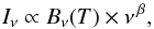 (9)where
β is a fixed emissivity spectral index, and
Bν(T) is the Planck
radiation law for temperature T. The parameters (T,
β) merely describe the properties of the observed radiation. In the
case of real observations, these would be called the colour temperature and the apparent
spectral index to emphasise the difference to the actual physical temperature and emission
properties of the dust grains. In the rest of the paper, we refer to the colour
temperature simply with the symbol T. We add pure Gaussian, uncorrelated
noise to the calculated intensities. In the first tests the relative noise is fixed to
either 5% or 10% of the original noiseless signal. We use two combinations of wavelengths.
The first one consists of 100.0, 160.0, 250.0, 350.0, and 500.0 μm, in
correspondence to a possible set of wavelengths observed with Herschel.
The second set is 100.0, 350.0, 550.0, and 850.0 μm. These wavelengths
were used in Planck Collaboration (2011) where the
data consisted of the IRAS 100 μm maps and the three highest frequency
bands of the Planck satellite.
(9)where
β is a fixed emissivity spectral index, and
Bν(T) is the Planck
radiation law for temperature T. The parameters (T,
β) merely describe the properties of the observed radiation. In the
case of real observations, these would be called the colour temperature and the apparent
spectral index to emphasise the difference to the actual physical temperature and emission
properties of the dust grains. In the rest of the paper, we refer to the colour
temperature simply with the symbol T. We add pure Gaussian, uncorrelated
noise to the calculated intensities. In the first tests the relative noise is fixed to
either 5% or 10% of the original noiseless signal. We use two combinations of wavelengths.
The first one consists of 100.0, 160.0, 250.0, 350.0, and 500.0 μm, in
correspondence to a possible set of wavelengths observed with Herschel.
The second set is 100.0, 350.0, 550.0, and 850.0 μm. These wavelengths
were used in Planck Collaboration (2011) where the
data consisted of the IRAS 100 μm maps and the three highest frequency
bands of the Planck satellite.
We have analysed observations of a small number of sources. Apart from the effects of
noise, the (T, β) values of the sources are assumed to
follow a single β(T) relation. For this relation we
selected a functional form 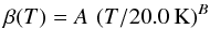 (10)(see,
e.g., Désert et al. 2008; Paradis et al. 2010; Planck
Collaboration 2011). For parameter B, we use the values of
− 0.3, 0.0, or +0.3. A negative value of B seems more consistent with
most observations, but we also examine a flat relation (B = 0.0) and a
positive T − β correlation (B = + 0.3)
to see the behaviour of the analysis methods in these different situations. To be roughly
consistent with the data on very dense clouds (for any of the chosen values of
B), the parameter A was fixed to a value of 2.2. In
most tests, we used a sample of 50 sources with temperatures distributed regularly between
8.0 K and 20.0 K. To build statistics, we typically examine 40 noise realisations of each
set of observations.
(10)(see,
e.g., Désert et al. 2008; Paradis et al. 2010; Planck
Collaboration 2011). For parameter B, we use the values of
− 0.3, 0.0, or +0.3. A negative value of B seems more consistent with
most observations, but we also examine a flat relation (B = 0.0) and a
positive T − β correlation (B = + 0.3)
to see the behaviour of the analysis methods in these different situations. To be roughly
consistent with the data on very dense clouds (for any of the chosen values of
B), the parameter A was fixed to a value of 2.2. In
most tests, we used a sample of 50 sources with temperatures distributed regularly between
8.0 K and 20.0 K. To build statistics, we typically examine 40 noise realisations of each
set of observations.
3.2. Radiative transfer model
As a more realistic set of simulated observation, we use surface brightness maps that are calculated with three-dimensional radiative transfer modelling, using a density field obtained from a magnetohydrodynamical (MHD) simulation.
The surface brightness maps are based on the MHD simulations of Padoan & Nordlund (2011) that were carried out on a grid of 10003 cells. For radiative transfer modelling the density field was regridded onto a hierarchical grid (see Lunttila & Juvela 2012), and the temperature distribution of the large grains was solved. The calculations resulted in 1000 × 1000 pixel surface brightness images. The dust model corresponded to normal Milky Way diffuse interstellar dust (RV = 3.1) as described in Draine (2003). The MHD model and the radiative transfer calculations have been described in detail in Juvela et al. (2012a). There the original cloud corresponded to a linear size of 6 pc and a mean hydrogen density of ~200 cm-3, but only the cloud opacity is important for modelling dust emission. For the present study we selected a smaller region that covers approximately one quarter of the projected area of the full model. The surface brightness images at 160 μm, 250 μm, 350 μm, and 500 μm were down-sampled to 101×101 pixel images with an assumed pixel size of 6″. We added to the images noise using as a starting point noise values of 3.7, 1.20, 0.85, and 0.35 MJy sr-1 per Herschel beam, assuming beam sizes 12.0″, 18.3″, 24.9″, and 36.3″, respectively. The noise level was adjusted with parameter N in the range of 0.0–1.0 times the default values. For analysis the maps were convolved to a common resolution of 40″.
3.3. Herschel observations
The final tests will be carried out using actual Herschel data at 160 μm, 250 μm, 350 μm, and 500 μm. The observations are for the field G109.80+2.70 that was analysed in Juvela et al. (2011) using the χ2 method (the target PCC288 in that paper). The data used in this paper are not identical. The observations of the SPIRE instrument, 250 μm–500 μm, have been reprocessed using the Herschel interactive processing environment HIPE v.9.02, with specific processing to improve the subtraction of the scan baselines. The SPIRE maps are the product of direct projection onto the sky and averaging of the time-ordered data. The 160 μm data of the PACS instrument have been processed with HIPE and the final map has been produced with the Scanamorphos program (Roussel 2012). The PACS map still suffers from some artefacts. The surface brightness appears to rise too much towards the northern corner of the map and, according to comparison with IRAS and AKARI data of the region, the 160 μm map also suffers from a small south-north gradient. Instead of correcting or masking the artefacts, we use the data directly in our comparison of the analysis methods. The zero point of the surface brightness scale has been estimated with the help of Planck and IRAS data (see Juvela et al. 2011, 2012b), and all data were convolved to 40″ before the analysis. The noise levels were estimated by selecting a flat region in the northern part of the map and by calculating the standard deviation between the observations and the same map convolved to a resolution of 2′. The noise per a 40″ beam was found to be 6.75, 4.34, 2.30, and 1.21 MJy sr-1 for the four bands in order of increasing wavelength. After masking areas outside and near the boundaries of the PACS map, we are left with an area of ~10′ × 10′. When sampled at 12″ intervals, the data set consists of ~7850 pixels at each wavelength.
The methods used in the estimation of the β(T) relation.
4. Results for idealised modified black body spectra
In this section we examine a series of simulated observations where, apart from the noise, each observed spectrum follows the assumed model of a modified black body exactly. We compare the results for the methods listed in Table 1 but do not include calibration factors δ yet in the calculations with the HM method. In Sect. 4.1, we use observations with fixed relative uncertainty for all bands and sources. In Sect. 4.2 we study the effect of analysing the low and high temperature sources separately. We then move to cases where the absolute uncertainty is fixed, emulating data from the current Herschel and Planck observations more closely (Sect. 4.3). In Sect. 4.4 we check the effect of the size of the source sample before, in Sect. 4.5, examining a case where the source temperatures are distributed according to normal distribution rather than uniformly between 8 K and 20 K.
4.1. Observations with fixed relative error
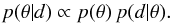
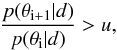
Figures 1–5 show examples of the results obtained with the χ2, SIMEX, BM, MC, and the HM methods when observations made at Herschel wavelengths have a constant signal-to-noise ratio across all bands and sources. The data consist of measurements of 50 sources with temperatures uniformly distributed between 8 K to 20 K and with the spectral indices following the β = A(T/20)B law with values of A = 2.2 and B = −0.3. The relative noise in the measurements is 5%. The figures indicate the β(T) relations recovered by each of the methods and the temperature and spectral index errors of individual sources.
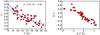 |
Fig. 1 The result of the χ2 method for the case where the sources follow a β(T) relation with parameters A = 2.2 and B = −0.3 and the measurements in Herschel bands have a relative noise of 5%. The left-hand frame shows the estimated T and β values and the fitted β(T) relation. The right-hand frame shows the absolute errors in the T and β values of the sources. |
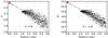 |
Fig. 2 The results of the SIMEX method for the same case as in Fig. 1. The points correspond to the A and B values derived in simulations of varying noise level. The red circles indicate the final values obtained by an extrapolation to a noise level of zero. |
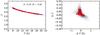 |
Fig. 3 The results of the MC method for the same case as the previous figures. Left frame: MC estimates of the T and β values. The red circles show the average parameters for each source. The dots represent 1000 MCMC samples, with the colours corresponding to different sources. The dashed black line is the true β(T) relation, and the solid blue line is the estimated relation. Right frame: absolute errors in the T and β values of individual sources. The dots correspond to 1000 MCMC estimates for the parameters of each source, and the solid red circles are the average values. |
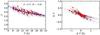 |
Fig. 4 The results of the BM method for the same case as in the previous figures. The contents of the frames are as in Fig. 3. |
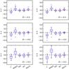 |
Fig. 6 Comparison of the errors in the recovered parameters A (left-hand frames) and B (right-hand frames) of the β(T) relation. The observations consist of measurements at 100, 160, 250, 350, and 500 μm, with a relative noise of 5%. The true value of B is indicated in the frames. |
Figures 1–5 all correspond to the same one realisation of observational noise. Some differences are already visible between the methods, but we must examine several noise realisations to estimate the bias of the methods.
In the following figures we compare the error distributions in the cases the different methods. Each synthetic set of observations consists of data on 50 sources. We derive the parameters A and B for 40 data sets that contain different realisations of observational noise. The scatter of the obtained parameter values provides crude estimates of the error distributions of the parameters A and B. Because each individual realisation already consists of observations of 50 sources, the variation in the estimated parameters remains small. This gives us confidence that the data set is sufficient to derive conclusions on the relative performance of the methods.
Figures 6 and 7 show the results for the analysis of simulated observations at 100, 160, 250, 350, and 500 μm. The figures correspond, respectively, to cases where the relative uncertainty of the measurements is either 5% or 10%. The plots show the distributions of the A and B parameter values relative to the true value in the simulations. The boxplots show the errors in the recovered parameters A and B for the methods: χ2, SIMEX, MC, BM, and HM(S). The boxplots show the median value of the recovered parameter (horizontal line inside the boxes), the range of values from the first to the third quartile (the height of the box), and the outliers (crosses) that are more than 1.5 times the extent of the inner quartile range (the distance shown as vertical lines or “whiskers”) outside the box. Figures 8 and 9 show corresponding results for observations at 100, 350, 550, and 850 μm. The relative noise of the measurements is again either 5% or 10%.
In Figs. 6–9 the behaviour of the methods MC and BM is very similar to each other. The parameters A and B are both slightly underestimated, although this is clear only in the case of the larger relative error. The bias of the hierarchical models has similar magnitudes but the sign of the bias tends to be opposite to the sign of B.
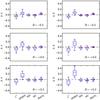 |
Fig. 8 As Fig. 6 but showing results for observations at 100, 350, 550, and 850 μm with a relative noise of 5%. |
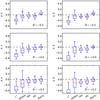 |
Fig. 9 As Fig. 8 (observations at 100, 350, 550, and 850 μm) but showing results for a relative noise of 10%. |
4.2. Analysis of smaller temperature ranges
We examined the observations of the previous section and also split them to two samples with temperatures above and below 14 K. The narrower dynamical range should make it more difficult to reliably estimate the β(T) relation. In particular, we are interested in the performance of the hierarchical model because it includes a global model for the distribution of the (T, β) values.
Figure 10 shows the errors of the recovered A and B parameters for χ2, SIMEX, BM, MC, and HM(S) methods. The full set of observations consists of 50 sources with a fixed relative uncertainty of 5% for intensity measurements at 100, 160, 250, 350, and 500 μm, following the β(T) law with B = −0.3. The results are shown for the 25 sources with temperatures in the range 8–14 K, the other 25 sources in the range 14–20 K, and for the combined sample of 50 sources. The statistics are based on 30 noise realisations. As previously, (e.g., Figs. 6–9) in the case of the same value of B, MC and BM show a small negative bias and the HM(S) a slightly larger positive bias. This applies to both the A and B parameters.
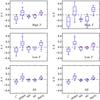 |
Fig. 10 The accuracy of the parameters of the β(T) relation for sources in different temperature ranges. The results are based on measurements at 100, 160, 250, 350, and 500 μm with 5% relative noise and a β(T) relation with B = −0.3. The high and low temperature ranges correspond to temperatures above and below 14 K. The bottom frames show the results for the combined sample. |
4.3. Observations with a fixed absolute sensitivity
In this section we adopt noise levels that are more in line with actual observation with Herschel and Planck. In the case of Herschel, we start with the sensitivities of 8.1, 3.7, 1.20, 0.85, and 0.35 MJy/sr at the wavelengths of 100.0, 160.0, 250.0, 350.0, 500.0 μm, respectively (as in Malinen et al. 2011; Juvela & Ysard 2012a). For extended emission, the noise per unit area would be relatively smaller at the short wavelengths because of the smaller beam size. However, we use the ratio of the values listed above directly, which is more appropriate for point-like sources, but which also accentuates the differences in the signal-to-noise ratios between the wavelengths. Similarly, for IRAS 100 μm and Planck data at 350.0, 550.0, and 850 μm, we start with uncertainties of 0.06, 0.12, 0.12, 0.08 MJy sr-1 (as in Juvela & Ysard 2012a). The actual noise levels are fixed by setting the signal-to-noise ratio to a value of 40 at the wavelength of 350 μm. At the other wavelengths, the signal-to-noise ratio varies depending on the source temperature and the β(T) law. In particular, the signal-to-noise ratio becomes low for the coldest sources and the shortest wavelengths (see Fig. 11).
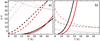 |
Fig. 11 The signal-to-noise ratio of the simulated observations of Sect. 4.3 as a function of the source temperature. The left-hand frame corresponds to the simulated Herschel observations at 100 μm (solid line), 160 μm (dashed line), 250 μm (dash-dotted line), and 500 μm (dotted line). The right-hand frame shows the signal-to-noise ratios for the simulated IRAS 100 μm data (solid line) and the Planck 500 μm and 850 μm bands (dashed and dotted lines, respectively). The signal-to-noise ratio of the 350 μm observations is 40. The black lines correspond to the relation β = 2.2(T/20.0)-0.3 and the red lines to β = 2.2(T/20.0)+ 0.3. |
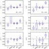 |
Fig. 12 The errors of the parameters of the β(T) relation in case of Herschel observations with fixed absolute noise levels. |
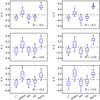 |
Fig. 13 The errors of the parameters of the β(T) relation in the case of IRAS and Planck observations with fixed absolute noise levels. |
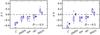 |
Fig. 14 Comparison of the errors in the A and B parameters of the β(T) relation, comparing cases with 50 or 500 observed sources. The methods of analysis are χ2, SIMEX, BM, MC, and HM(S). For each method, two boxplots are shown, the 50-source case on the left and the 500-source case on the right. The observations consist of data in Herschel bands at wavelengths 100–500 μm and with a relative noise of 10%. |
The accuracy of the recovered parameters of the β(T) relation are shown in Figs. 12 and 13, for the Herschel and the Planck cases, respectively. The results of the SIMEX method are often poor and fall partly outside the plotted range. This appears to be caused by the very low signal-to-noise ratio of some sources that, when the noise is further increased, leads to outliers that destroy the accuracy of the extrapolation. The situation might be improved by using larger set of noise realisations and, in the fits of β(T), replacing the least squares with a more robust fitting routine. For the other methods, the results are consistent with the previous tests with fixed relative measurement uncertainties. BM and MC are close to each other. The same applies to the pair of HM(N) and HM(S). However, the hierarchical models show somewhat higher bias and, unlike in Figs. 6–9, the bias in the parameter B is always positive irrespective of the true value of B.
4.4. The effect of the number of sources
In this section, we examine how the number of observed sources (or pixels) affects the results. For this purpose, we generated data consisting of 500 sources with temperatures uniformly distributed between 8 K and 20 K, and the spectral index following Eq. (10) with A = 2.2 and B = −0.3. Figure 14 compares the results obtained with methods χ2, SIMEX, BM, MC, and HM(S) when applied to data in the Herschel bands at wavelengths 100–500 μm and with a relative noise of 10%. Ten realisations are used in this case, and the results are compared with the 50-source cases with the same number of realisations.
As expected, the scatter in A and B values is significantly smaller in the case of 500 sources, because of the averaging of the statistical noise. More interestingly, all methods also exhibit smaller bias. This is particularly true for the χ2 and SIMEX methods, SIMEX having almost no bias left. The HM(S) method also performs better, producing results compatible with the true values of A and B. The MC and BM results are more robust regarding the source numbers, the variation in bias between the 50- and 500-source cases being compatible with the scatter of results.
4.5. The effect of the distribution of source temperatures
The hierarchical model includes the implicit assumption that the joint probability distribution of I, T, and β can be described as a multidimensional normal distribution (version HM(N)) or as Student distribution (version HM(S)). By using sources whose temperatures are distributed uniformly between 8 K and 20 K, we are clearly inconsistent with this assumption. To see whether this has an effect on the results, we examined a case where the source temperatures are extracted from a normal distribution with a mean value of 14.0 K and a standard deviation of 3.0 K, the values being restricted to the same range 8.0–20.0 K.
Figure 15 compares the cases between uniformly and normally distributed source temperatures. The results are shown for the BM, HM(N), and HM(S) methods when the relative noise at Herschel wavelengths is 10%. Each simulated set of observations consists of 50 sources. Figure 15 is based on data from 30 noise realisations. In the case of the hierarchical models, the results do not indicate any clear dependence on the form of the temperature distribution. Because the normal distribution also means an actually narrower dynamical range of temperatures, it may even suggest that the loss of dynamical range is compensated for by the better match with the assumptions of the method, which include the normal distribution of temperature values. However, it is clear that the bias and the dispersion of the parameter estimates are not strongly affected by the change in the temperature distribution. The only noticeable effect is the marginally larger bias of the BM results when the distribution of source temperatures follows normal distribution.
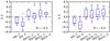 |
Fig. 15 Comparison of the errors in the A and B parameters of the β(T) relation, comparing cases where the source temperatures follow a uniform (U) or a normal (N) distribution. The compared methods of analysis are BM, HM(N), and HM(S). The observations consist of data in Herschel bands at wavelengths 100–500 μm and with a relative noise of 10%. |
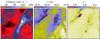 |
Fig. 16 The 250 μm surface brightness, dust colour temperature, and spectral index maps for the MHD model cloud. The values correspond to the χ2 solution with noiseless data. |
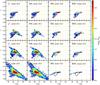 |
Fig. 17 The distributions of (T, β) values for different methods (χ2, BM, HM(N), and HMC) and for the MHD model and noise levels N = 0.0–0.5. The values are the Bayesian estimates of the individual pixels.To guide the eye, a single contour following the solution for the N = 0.0 case is plotted in each frame. The colour scale corresponds to logarithmic number of pixels per a (T, β) interval. |
5. Results for a radiative transfer model
In this section we analyse synthetic surface brightness data that are obtained with MHD simulations and radiative transfer modelling (see Sect. 3.2). The comparison is mainly restricted to χ2, BM, and HM(N) methods. We also examine the effects of mapping artefacts and calibration errors. To this end, we carry out calculations using HM including free parameters for the relative calibration of the observed bands. This variation in the HM method is denoted as HMC.
Figure 16 shows the temperature and spectral index maps calculated with the χ2 method using noiseless data (N = 0.0). The colour temperature ranges from 15.36 K to 17.01 K, with lower temperatures being found towards regions of higher column density. The values of the observed spectral index are between 1.82 and 2.13, the low values also being associated with dense regions. In the model, the intrinsic emissivity spectral index of dust grains themselves was constant, close to the observed maximum value. In observations, the deviations from the intrinsic value result from line-of-sight temperature variations that tend to decrease the apparent spectral index deduced from observed intensities. In the fit, the different bands were weighted according to the noise values given above. Although these data contain no noise, the relative weighting may slightly affect the results because the simulated intensities do not precisely follow a modified black body law. Still, we consider these maps as references to which all methods are compared. The top left-hand panel of Fig. 17 shows the T − β distribution of these maps. Two main features characterise the maps. Firstly, there is a tight T − β correlation for most most pixels, these corresponding to areas of lower column density and relatively high values of both T and β. The second feature corresponds to a smaller number of pixels that are found in regions of high column density and that have lower values of T and especially of β.
Figure 17 shows the distribution of the recovered (T, β) values for the χ2, BM, and HM methods for noise levels N =0.0, 0.1, 0.2, and 0.5. When the input data contain no noise, N = 0.0, the calculations were completed using error estimates corresponding to the N = 0.1 case. This was done because the calculations are technically not possible if error estimates are zero. The values plotted in Fig. 17 are the Bayesian estimates of each map pixel, which are the mean values of the corresponding parameter values in the MCMC chains.
Unlike in Sect. 4, the results of χ2 and BM are almost identical. Section 4 discussed the relative bias between sources of different temperatures while data in Fig. 17 correspond to a narrow temperature range (see Fig. 16). Over an interval of ΔT = 1.0 K a bias of ΔB = 0.1 corresponds to a change of less than 0.01 in the spectral index, too small to be noticeable. Furthermore, in Fig. 17 the noise level is lower, especially relative to the 10% relative noise case of Sect. 4. Asymmetries in the distribution of χ2 values are also usually stronger at lower temperatures and, because the temperature and spectral index values of Fig. 17 are well within the range allowed by the flat priors, the priors are not expected to cause any differences either.
Unlike BM, HM show positive correlation between T and β up to the highest noise level. For N = 0.1, the covariance matrix of the model implies a correlation coefficient of 0.69 between these parameters, which decreases to 0.52 for N = 0.5. At both noise levels, the model covariance matrix gives a standard deviation for β of ~0.015, while pixels with values below β = 2 only exist at the lower noise level. Therefore, the difference in the distribution of β values is not caused by a significant change in the global part of the hierarchical model but rather directly by changes in the relative weight given for the likelihood function.
Figure 18 compares the results of BM and HM(N) in case of noise levels N = 0.1 and N = 0.2. The plots shows the behaviour emphasising regions with low T and β values. One should note that the pixels with T < 16.0 K and pixels with β < 2.05 represent only a small fraction of the full map, ~8% and ~2%, respectively. On the other hand, by being associated with dense cloud structures, the signal-to-noise ratios of those pixels are higher than average. Figure 18 shows that HM provides significantly lower scatter at both noise levels, and this results in more accurate temperature estimates. However, the HM results also contain bias whereby the spectral index β is overestimated for pixels with low β. These also are the pixels with the lowest temperatures.
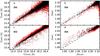 |
Fig. 18 The parameters estimated from noisy data versus the true values obtained from noiseless observations. The upper frames correspond to the BM method and the lower frames to the HM method. In each frame, black and red points correspond, respectively, to the noise levels of N = 0.1 and N = 0.2. |
The results may depend not only on the level of noise but also on the assumption of the probability distributions that are used in the analysis. Figure 19 shows the distributions of (T, β) values for the HM(N) method and noise level N = 0.1. The second frame corresponds to the HM(S) method (i.e., using Eq. (6) instead of Eq. (5)). The use of the Student probabilities results in a solution where all pixels fall onto an narrow band in the (T, β) plane. The difference was confirmed repeating the calculations with different initial values. However, for the lowest temperature pixels, which also correspond to the lowest β values, the convergence of the MCMC chain is slow, requiring several millions of MCMC steps.
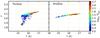 |
Fig. 19 Distribution of recovered Tand β values for MHD model with noise N = 0.1 and the HM method with probabilities being calculated either with normal distribution (left-hand frame) or with Student distribution (right-hand frame). The colour scale corresponds to logarithmic number of pixels per (T, β) interval. |
5.1. Effects of noise and calibration errors
In Fig. 17 we, for the first time in this paper, include results from hierarchical models that include parameters δ to account for calibration errors. The model includes three additional parameters, δi, the relative scaling factors of the 160 μm, 350 μm, and 500 μm data. Together these three factors can compensate for any change in the spectral index; i.e., β is completely degenerate with these parameters. To obtain a unique solution, we use Gaussian priors with a mean value of 0.0 and standard deviation 0.001 for log 10δi.
The calibration factors are strongly constrained to remain near the default value of 1.0 but are, nevertheless, found to deviate from this value even when the input data contain no actual calibration errors. This is caused by the model emission not following a modified black body law. The line-of-sight temperature variations tend to broaden the emission spectrum, but here they only play a minor role. The main cause lies in the opacity of the employed dust model that does not follow a single νβ relation (Draine 2003). Figure 20 demonstrates the deviations of the model spectra relative to the fitted modified black body spectra. In HMC, these are interpreted as errors (no longer necessarily calibration errors) relative to the assumed spectral model. Because each data set consists of more than 10000 pixels, the priors of the parameters are not strong enough to force the values log 10δi to zero.
The results of HMC method do not behave quite consistently as a function of the noise level. This must be partly related to the changes in the influence of the δi priors for cases of a different noise level. However, it also might indicate some problems in the convergence of the calculations. For some initial values, the N = 0.5 calculation appeared to result in a solution that was ~0.1 below the correct β value or that gave very nearly the same β value for all pixels. This suggests that the burn-in phase can be very long, and even after some tens of million MCMC steps, the calculations have not yet really converged. This is likely to affect mostly noisy observations where the probability maximum is less well defined. The common feature of all the solutions was that, as the noise increases, instead of forming a separate group with clearly lower β values, the low temperature pixels begin to conform with the general distribution dictated by the majority of the pixels.
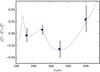 |
Fig. 20 Deviations from the fitted modified black body law in the case of the MHD model. The plot shows the relative deviations for 5% of the highest (blue symbols) and 5% of the lowest column density (black symbols with larger error bars) pixels. The error bars correspond to noise per pixel for the general noise level N = 0.1. The dotted line shows relative deviations between a ν2.1 dependence and the actual opacity in the employed dust model. |
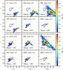 |
Fig. 21 The distributions of (T, β) values for data containing calibration errors where either 160 μm data (first six frames) or the 350 μm data (six last frames) has been scaled by 1.1. The methods are χ2, BM, HM, and HMC, the last one corresponding to a hierarchical model that includes free parameters for multiplicative corrections in three bands. Each frame corresponds to one combination of method and statistical noise, as indicated in the frames. The single contour corresponds to the locus of the correct solution (see Fig. 17). |
We repeated the HMC calculations for simulations where the intensities of either the 160 μm or the 350 μm data were multiplied by 1.1. The applied calibration error is not particularly high but still several times larger than the differences seen in Fig. 20. The results are shown in Fig. 21 where, for comparison, we also plot results for selected χ2 and BM calculations. HMC is able to recover the (T, β) values quite well, especially when comparing with the other methods where the effect of the calibration error is clearly visible. With increased observational noise, the shape of the (T, β) distribution is distorted in a similar way to the cases in Fig. 17. Some positive correlation remains between temperature and spectral index, even at the noise level of N = 0.5. However, the precise shape of the distribution was found to depend weakly on the initial values, suggesting incomplete convergence of the calculations.
5.2. Effects of mapping artefacts
The MHD model simulations can be considered realistic concerning distribution of temperature and spectral index values. Because of the temperature variations in the model, deviations from the simplistic spectral model of a single modified black body are possible. However, these data are still idealised in the sense that they do not contain any large-scale artefacts that can be encountered in real observations.
We carried out one set of tests on the effects of mapping artefacts. We introduced a horizontal stripe in the 160 μm map by adding a constant value of 3 MJy sr-1 to the affected pixels and a similar vertical stripe in the 350 μm map by subtracting 2 MJy sr-1. The width of both stripes is 10% of the map size. As shown in Fig. 22, the artefacts are not strong enough to be visually prominent in the surface brightness data. The maps were analysed with the BM, HM, and HMC methods, with noise levels N = 0.1 and N = 0.2.
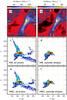 |
Fig. 22 The 160 μm (frame a)) and 350 μm (frame b)) surface brightness maps (N = 0.1) that include stripes with constant surface brightness offsets. The white lines indicate the widths of these stripes. Frames c) and d) show the distribution of (T, β) values obtained with HM for all the pixels (frame c)) and separately for the pixels outside the stripes (frame d)). Frames e) and f) show the corresponding results for method HMC. The black contours correspond to the distribution of values for method HM, in the case of no stripe artefacts and no noise (see Fig. 17). In frames c–f), the colour scale corresponds to logarithmic density of pixels per a (T, β) interval. |
The temperature and spectral index estimates are strongly affected within the modified areas, especially at low column densities where the fractional surface brightness changes are large. Figure 22 demonstrates that, unless the pixels affected by the stripes are removed, the general appearance of the (T, β) distribution is dominated by these artefacts. It is important to see whether the results for the remaining pixels are affected through the global part of the HM model. According to Fig. 22, there is only a small effect. Because of the additional free parameters, the stripes could bias the results of the HMC method more than the results of the HM method. However, in Fig. 22, there is no clear evidence of this either. Of course, if the area or amplitude of the artefacts is increased, more noticeable global effects should eventually appear.
6. Results of the analysis of Herschel observations
As the final test we carried out analysis of Herschel 160 μm, 250 μm, 350 μm, and 500 μm observations of the G109.80+2.70 (see Sect. 3.3). Figure 23 shows the 250 μm surface brightness map (a proxy for column density) and the temperature and spectral index maps derived with the χ2 method. The lower frames show the (T, β) values obtained with the χ2, BM, and HM(N) methods. For BM and HM(N) methods the priors are the same as in the previous MHD simulations (see Table 2). Unlike for example in Fig. 17, all methods show a negative correlation between T and β. The covariance matrix in the global part of the hierarchical model gives a value of − 0.82 for the correlation coefficient between T and β. The standard deviations are 0.058 K for T and 0.052 for β.
The limits of the priors used in MCMC calculations and in hierarchical models.
We emphasise that the results of Fig. 23 may be affected not only by noise but also by the mapping artefacts noted in Sect 3.3. The observed signal is further modified by line-of-sight dust-temperature variations that decrease β especially towards the embedded sources. Therefore, the observed β(T) relation cannot be used directly to infer the intrinsic opacity spectral index of dust grains. Nevertheless, we also show in Fig. 23 the results of the least square fitting of Eq. (10).
At 160 μm, the differences between the observed surface brightness maps and the χ2 fit are shown in Fig. 24. In addition to a weak large-scale gradient, there are some possible artefacts at the map boundaries. The SPIRE maps do not have any noticeable gradients relative to each other. In the fit the 160 μm map appears to be quite consistent with the 350 μm and 500 μm maps, while the 250 μm map is left with a significant positive offset. Of course, based on the four maps and without a priori knowledge of the dust spectral index (or temperature), it is not possible to say whether the 160 μm values are in reality too low or the 250 μm values too high or if the SPIRE channels favour a spectral index that is incompatible with the 160 μm data (e.g., because of the presence of several temperature components). The 160 μm residual map also highlights some smaller features where the relative intensity of the 160 μm is low, either in absolute or relative terms. These may not all be physically real features, but at least the relatively high 160 μm residuals towards the centre of the field can be easily explained by the presence of a warmer dust component associated with the embedded young stellar objects (Malinen et al. 2011; Juvela et al. 2011).
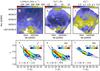 |
Fig. 23 Results for the Herschel field G109.80+2.70. The upper frames show the observed 250 μm surface brightness and the temperature and spectral index maps from the χ2 method. The lower frames show the distributions of the (T, β) values obtained with the χ2, BM, and HM(N) methods, the colour scale corresponding to logarithmic number of pixels per (T, β) interval. The solid lines are least square fits with the parameters A and B given at the bottom of each frame. |
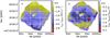 |
Fig. 24 The residuals between the observed 160 μm surface brightness in the field G109.80+2.70 and the χ2 fit. The residuals are shown both as absolute errors (left frame) and relative to the χ2 fit. |
Surface brightness data may suffer from at least two systematic effects, multiplicative errors in the surface brightness calibration and additive errors in the zero point of the surface brightness scale. Assuming that a modified black body spectrum is an accurate model of the emission, method HMC tries to correct for the multiplicative errors. However, additive errors may be an even more serious problem because they introduce systematic effects in temperature and spectral index that vary as the function of surface brightness, that is, depending on column density. Therefore, we also tested a hierarchical model where, instead of the multiplicative factors, the zero point offsets of the 160 μm, 350 μm, and 500 μm maps were taken as free parameters. The median surface brightness of these G109.80+2.70 maps were 181, 89, and 40 MJy sr-1, respectively. The priors of the offset corrections were taken to follow normal distribution with the standard deviation equal to 1% of the median surface brightness value. The results are shown in Fig. 25.
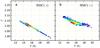 |
Fig. 25 The (T, β) distributions of the field G109.80+2.70 from hierarchical models that include multiplicative calibration factors (left frame) or zero point offsets (right frame) as additional parameters. |
In the fits, the additive corrections were + 5.7, + 6.3, and + 1.2 MJy sr-1 for the 160 μm, 350 μm, and 500 μm bands, respectively. For the 160 μm band this is consistent with Fig. 24, taking into account that there the residuals are relative to a fit that included the 160 μm data as input. The correction is also positive for the other bands, suggesting that the 250 μm input map has some positive offset with respect to the other bands. Because of the priors of the additive correction factors, the solution should be well defined. However, this does not eliminate the fact that the calibration correction and the derived spectral index are partially degenerate. According to Fig. 24, the relative errors are not very significant. This also is reflected in the multiplicative calibration factors that in our calculations were close to unity, 1.01, 1.05, and 0.98 for 160 μm, 350 μm, and 500 μm, respectively.
If data contains additive errors and model includes only multiplicative corrections, or vice versa, the solution will have errors that, as a function of the surface brightness level, behave in a complex fashion. The combination of models with both additive and multiplicative corrections is left for later studies. However, it is already clear that an increased number of parameters will not only make the calculations more time-consuming but also make them more sensitive to the underlying model assumptions. Problems like large-scale gradients and local mapping artefacts may be more significant, and they must be dealt with in a different way.
7. Discussion
We have examined five methods that can be used to estimate the shape of the β(T) relation based on multiwavelength dust continuum observations of a set of sources (or pixels). The χ2 fitting of the intensity values followed by χ2 fitting of the resulting (T, β) values, is known to lead to strongly biased results. Therefore, we particularly examined the bias exhibited by the other methods.
7.1. Analysis of idealised modified black body spectra
The performance of the methods was first examined using idealised observations where each spectrum consisted of a single modified black body and white noise. The results allowed us to to draw some conclusions on the accuracy and, in particular, on the bias in the results.
7.1.1. The SIMEX method
SIMEX is based on the general idea that while we do not have noiseless data available, we can examine how the results vary when the noise level is increased beyond that of the actual observations. The method is empirical, and there is no guarantee that the behaviour at low and high noise levels is similar so that a reliable extrapolation would be possible. The noise level of the observations must, of course, also be estimated, so that one knows how far the extrapolation should be extended. We modelled the noise dependence of the A and B values with linear functions. The results were partly disappointing. When the observations have 5% relative uncertainty, SIMEX overestimates the correction with the result that the bias is of the same order of magnitude as for the χ2 method but of opposite sign. The results were better when the observational noise was raised to 10%. For the SIMEX method, the higher noise did not significantly increase the bias, while in the χ2 fits it was higher by a factor of about 3–4 (as measured by the parameters A and B). Figure 2 suggests that the noise dependence is not entirely linear. This is definitely true close to the original noise because, as long as the added noise is small compared to the original noise, the bias should not change much. The reliability of the results will also depend on the range of noise levels examined, in our case one to three times the original noise. When the data included some observations with very low signal-to-noise ratio (Figs. 12 and 13, see Sect. 4.3), the SIMEX results were very poor. The use of SIMEX in the analysis of real observations would require a more systematic study of the extrapolation functions, the optimal range of noise values used, and the amount of Monte Carlo samples required. Our implementation may also have failed partly because of the non-robust nature of the employed least-squares fits. At lower noise levels, the systematic behaviour of the bias and the relatively small amplification of statistical errors suggest that some improvements over the results presented in this paper should be possible.
7.1.2. Bayesian model and the MC method
Compared to the χ2 and SIMEX methods, MCMC calculations of the basic Bayesian model (BM) were quite successful in eliminating the bias in the parameters of the β(T) relation. Nevertheless, the estimated values of the parameter B tended to be slightly too low. In other words, the results showed a small bias in the direction of the noise, towards a tighter anticorrelation (or looser positive correlation) between the temperature and the spectral index. The behaviour was similar in the case of observations with fixed relative noise as in the tests with fixed absolute noise. The values of T and β obtained for individual sources can show quite significant scatter (e.g., Fig. 4). However, for a sample of 50 sources, the statistical uncertainty of the B parameter was below ~0.1 units for all the examined noise cases. In the method MC, we explicitly enforce a single β(T) relation that, in this paper, also was assumed to have the correct functional form, β = A(T/20)B. If the assumption is true, this should result in a more powerful method of recovering the values of the parameters A and B. The effect of the noise is taken into account with separate Monte Carlo simulations, assuming that this can be reliably estimated.
Compared to the hierarchical models, this method has the advantage that we do not need to specify any model for the noise distribution of I, T, and β values. We simply use the error estimates of the intensity measurements and use Monte Carlo simulation to estimate the effect of the noise on the end result, which consists of the parameters of the β(T) relation. This could be useful if the noise induced dispersion of the T and β values cannot be described well with a covariance matrix. For low signal-to-noise ratios, the joint error regions are known to be strongly curved, the distributions of individual parameters are skew, and the (T, β) values themselves are biased. All these effects would be automatically taken into account, based on the error distributions of the intensity measurements. In practice, the performance of this MC method turned out to be very similar to that of BM. In particular, the method tended to underestimate the values of A and B, but the bias was typically no more than ΔB = −0.1 in the case of 10% relative noise and less than ΔB = −0.05 for the case with 5% of relative noise. In spite of the strong constraint regarding the functional form of β(T), the method did not clearly outperform the other methods. In the absolute noise case, Figs. 12 and 13, the MC method produced results quite comparable to BM but with smaller scatter in the T and β values. The same applies to the tests with 5% and 10% relative noise, although there the hierarchical models also performed rather well. On the other hand, the method MC is relatively slow because each step includes the fitting of modified black body curves for each source. In this method, the MCMC chains also were more likely to get stuck, because they have a very low rate of acceptance for the steps taken. This is directly related to the additional condition that forces the simulated A and B parameters to approach the observed values (see Sect. 2.5). The situation might be improved by adjusting the relative step size of the different Markov chain parameters. The method gives results with low statistical noise, but on the other hand, the scatter would remain small even if the sources did not follow the same β(T) law.
7.1.3. Hierarchical models
The remaining methods were based on the hierarchical model, using two alternative probability distributions. When the two version were compared (e.g., Figs. 12–15), the results were very similar. This is to be expected because of the idealised nature of our simulations and, in particular, the absence of outliers. In the tests with 5% and 10% relative observational noise, the results of the HM method appeared to be slightly biased towards a flat relation. In other words, the bias was negative when B was positive, and with a positive true value of B, the bias was positive. In the case of 5% relative noise, both A and B were recovered with typical bias below 0.05 units. For 10% of relative noise, the results were mostly correct to within 0.1 units. However, in the case of simulations with fixed absolute noise, the bias was increased. This is likely to be caused by the strong decrease in the signal-to-noise ratio towards the lower temperatures. The (T,β) relation is then mainly determined by the sources with a high signal-to-noise ratio, and the low-temperature part is extrapolated based on the assumed model for the joint (T,β) distribution. The same phenomenon was noted by Kelly et al. (2012) (see their Fig. 9). In this case, the hierarchical models show clear positive bias (see Figs. 12 and 13). Unlike in the previous cases with fixed relative noise, the sign of the bias no longer depends on the sign of B. The bias is similar for both the Herschel and Planck wavelength sets. For B = −0.3 the bias is ΔB = + 0.3 and thus, instead of recovering the decreasing β(T) function, the results would suggest a completely flat relation. This is in stark contrast to the BM and MC methods, which both slightly overestimate the steepness of the β(T) relation but still recover the correct sign of B.
Depending on the version, the hierarchical model tries to describe the distribution of temperature and spectral index values using either multivariate normal or Student distribution. Kelly et al. (2012) also examined cases where, contrary to this assumption, the distribution was bimodal. The method was not found to be sensitive to this deviation. We carried out a similar comparison between a uniform temperature distribution and a normal distribution and did not see any clear difference either in the bias or scatter of the temperature and spectral index values (see Fig. 15). In this paper, the default assumption was that of a uniform temperature distribution. Another difference to the Kelly et al. (2012) calculations is that while we have used directly the intensity and temperature values, they used in the fitting the logarithms of these variables. We tested the difference between the use of linear and logarithmic scales. For the cases with 5% and 10% relative noise, we do not see any difference in the results obtained with linear and with logarithmic variables. In the case of absolute (and, for some sources and wavelengths, larger) errors, there is a small difference (see Fig. 26). However, these differences, if real, are still small compared to the differences to, say, the BM and the true values. While the (T, β) values follow a non-linear relation, the same also applies to (lg T, β).
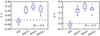 |
Fig. 26 Comparison of results of different versions of the hierarchical methods, HM(N), HM(S), and HM(SL) where the last one fits the intensity and temperature on a logarithmic rather than at a linear scale. The observations consist of Herschel wavelengths with the absolute errors as described in Sect. 4.3. |
We have examined only a few examples of the wide category of hierarchical models. It should be possible to develop the methods further, to better take the details of noise effects into account and to accommodate rare sources whose properties differ from the average. In comparing the Bayesian point estimates, we also have not made full use of the information provided by MCMC, which includes the shape and extent of credible regions. With these considerations, and possibly in the case of larger sample sizes, hierarchical models may appear in an even more favourable light.
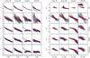 |
Fig. 27 Comparison of the derived (T, β) values in the case of simulated modified black body spectra of different noise level (cf. Sect. 4). The black solid lines correspond to the relation assumed in the simulation of the observations. The measurements have 5% or 10% relative errors or the absolute errors described in Sect. 4.3. In the fourth column of frames, the observations follow two distinct β(T) relations (black solid lines) with 20% relative errors for the low temperature branch (T < 15 K) and 5% relative errors for the high temperature branch (T > 14 K). The left-hand frames show some MCMC samples (coloured dots), their averages (red circles) and the fitted β(T) relations (dashed blue lines). The right hand frames show the distributions for the errors ΔT and Δβ. The plots correspond to a single noise realisation of observations of 50 sources. |
7.2. Distributions of T and β values
In connection with the simulated modified black bodies, we concentrated mainly on the bias of the T(β) relation. However, the scatter of the individual (T, β) values is equally important. In Fig. 27 we plot examples of this scatter in the case of MC and BM methods and three variations of the hierarchical models. The hierarchical models use either normal or Student probabilities and, in the latter case, the fitted parameters are either intensity and temperature or their logarithms. This last alternative is marked as HM(SL). The figure shows the results for one realisation of the observations of 50 sources. The columns of the figure correspond to different noise cases. In the fourth column of Fig. 27, the 25 sources below 15 K also follow a different β(T) law from the 25 sources above 14 K. The parameters are A = 1.8 and B = −0.3, but β for the higher temperature branch is calculated using variable T−6 K instead of T. The relative noise is 20% for the low temperature and 5% for the high temperature branch.
BM exhibits the largest scatter of individual (T, β) values, but the average estimates are not strongly biased. This applies even to the case of two β(T) relations (fourth columns) because the fits of the sources are independent from each other. The hierarchical models exhibit a significantly smaller scatter, but the results are occasionally more biased. The bias is usually towards a flat β(T) relation. Furthermore, when the data include some observations that have higher noise and follow a different relation from that of the high signal-to-noise data, the apparent result is a single β(T) relation that also exhibits a relatively small scatter. In the case of real observations, the sources are unlikely to follow a single β(T) law and one must be cautious in interpreting the results as a proof of such behaviour. The MC method (uppermost frames in Fig. 27) is the extreme case where, by construction, the results will fall on a single β(T) relation whose functional form is predefined. Thus, the results will show a single relation irrespective of the validity of the assumption.
For hierarchical models, the variation in the observational noise is not reflected in the scatter of the (T, β) estimates as strongly as in the case of BM. This is particularly noticeable in the absolute noise case and in the case of the two β(T) relations where the signal-to-noise ratio is lower for the colder sources. The information of the high signal-to-noise sources is extrapolated effectively to the low signal-to-noise sources. Depending on the case, this may cause significant errors. In particular, in the case of two β(T) relations of Fig. 27, all points incorrectly appear to fall onto a single β(T) relation. This suggests some caution when interpreting such results.
7.3. Results of the radiative transfer models
In the MHD models of Sect. 3.2, the range of temperatures was much narrower than in the previous tests. Instead of trying to estimate a functional form of the T(β) relation, we only examined the general distribution of the (T,β) values. Compared to the constant 5% or 10% relative uncertainties of Sect. 4.1, the signal-to-noise ratio of the simulated surface brightness maps varied by a factor of ~30 across the map (see Fig. 16), the median being ~13 for 250 μm and N = 1.0. For the brightest regions, the signal-to-noise ratio exceeds 100, and these regions strongly influence the overall solution of the hierarchical models.
The BM calculations included flat priors with very wide ranges of allowed parameter values (see Table 2). As a consequence, little difference was seen between the χ2 and BM solutions, even for the tails of the distribution that correspond to data with low signal-to-noise ratios (see Fig. 17). The relatively high average temperature also contributes to this result because the noise-induced error regions tend to become strongly asymmetric only at lower temperatures. One should remember that the bias discussed in Sect. 4 concerns the relative errors at different parts of the T(β) relation, while here, in the absence of noise, all pixels fall in a temperature interval that has a width not much more than 1 K.
For the hierarchical models, the results are consistent with those discussed in Sect. 7.2. The global part of the hierarchical models helps to suppress the noise-induced anticorrelation between temperature and spectral index. In Fig. 17, HM and HMC methods give results where, even when the noise increases, all pixels fall close to the correct solution. In the χ2 and BM solutions the same applies to the highest signal-to-noise pixels but the figure emphasises the overall scatter that is dominated by the low intensity regions. In the hierarchical models the global part of the model forces those regions to follow the distribution of the high signal-to-noise data. The result is a very tight distribution which is good solution, provided that all pixels behave statistically in a similar fashion. However, this is not quite true in the case of the MHD model. The coldest regions also have the strongest line-of-sight temperature variations, and as a consequence, they deviate from the general T − β -trend (see also Shetty et al. 2009b; Juvela & Ysard 2012b). In Fig. 17 these regions form a separate cloud of points below β = 2.0. The hierarchical models perform very well up to noise level N ~ 0.2. When noise is further increased, the low-β points are forced to follow the general trend; that is, their spectral indices are overestimated and temperatures underestimated. In the BM solution, the (T, β) values of these pixels appear to be more unbiased, but the overall distribution is strongly deformed by the noise already at N = 0.2.
When the data were modified to include calibration errors, all temperature and spectral index values were affected. At 160 μm a 10% calibration error corresponded to a shift of ΔT ~ 2 K and Δβ ~ 0.2 (see Fig. 21). A similar fractional error at 350 μm had almost no effect on temperature and also changed the spectral index estimates only by ~0.1. When the hierarchical model included parameters for possible calibration errors, the method was able to recover the correct (T, β) values almost as well as before the calibration errors were included. However, at higher noise levels, also the bias in the low-β pixels was as noticeable as in Fig. 17.
The experiment with mapping artefacts demonstrated that, even when the artefacts are barely noticeable in surface brightness data, they can easily dominate the appearance of the overall (T, β) distribution (see Fig. 22). In our test, the stripes did not significantly affect the results outside the artefacts themselves. However, if it is possible to identify artefacts in the input maps (e.g., based on fit residuals), it is always safest to discard them from the analysis with hierarchical models.
7.4. Analysis of Herschel maps of G109.80+2.70
The results for the Herschel field G109.80+2.70 were presented in Sect. 6. In this case the true solution (i.e., in the absence of noise and possible calibration errors and mapping artefacts) is not known. Nominally the average signal-to-noise ratio of these data is even higher than in the case of the MHD models. In the brightest regions the 250 μm surface brightness exceeds 400 MJy sr-1, while the noise (estimated at low surface brightness) is lower by a factor of ~100. On the other hand, the data appeared to contain some gradients and local artefacts, which are errors that cannot be described easily with any global parameters.
For χ2 and BM methods, the dispersion of the (T, β) values was again rather similar, although this time the locus of the BM solution corresponded to slightly higher temperature and lower spectral index (see Fig. 23). The difference should correspond to the difference between the maximum likelihood estimates and the Bayesian estimates that are averages over MCMC samples. Because the prior distributions were flat over a wide range of parameter values, the priors should not have a noticeable effect in Fig. 23. The Bayesian MCMC estimates are often considered more robust. However, there also are situations where the maximum likelihood estimates can be more accurate. One example was shown in Juvela & Ysard (2012a) (see Fig. 2 in that article), where the noise induced in the probability distribution a long tail to lower temperatures and higher values of the spectral index. In that case the maximum likelihood was reached close to the correct values, while the mean of the probability distribution would be biased. In G109.80+2.70, the hierarchical model again produced the smallest scatter in the (T, β) values, although the difference between the methods was smaller than in the previous MHD models.
We considered alternative hierarchical models with either additive or multiplicative correction factors for the calibration. Both resulted in similar temperature values but the derived spectral indices were higher by more than 0.05 when additive corrections were used. The results were positive, at least in the sense that including the calibration factors did not lead to widely different results. However, without strong priors on the calibration factors, the solution could result in very different values of spectral index or even divergence. One cannot unreservedly advocate including of calibration factors as part of routine analysis. The correction is based on the assumption that the observed radiation follows a modified black body law. This is known to be only an approximation (because of more complex wavelength dependence of dust opacity and temperature variations within the telescope beam). The derived calibration factors may also be affected by possible mapping artefacts, that is, local features that cannot be properly taken into account by global parameters. It is always useful to examine the residuals between the surface brightness data and the model fits, whether calibration errors are included in the model or not. In hierarchical models, it is better to mask the problematic regions rather than take the risk that the whole solution is affected.
All the methods applied to the G109.80+2.70 data agreed on a general anticorrelation between T and β parameters. The simulation of Fig. 22 acts as a warning example how strongly the apparent relation between T and β can be affected by small imperfections in the data. Nevertheless, we are confident that the anticorrelation is real in G109.80+2.70. This is at least partly connected with temperature variations caused by young stellar objects embedded in a cold clump (see Juvela et al. 2011 for a toy model of the field). The correlations between T and β in G109.80+2.70 and other fields observed in the project Galactic cold cores (Juvela et al. 2012b) will be analysed in more detail in future papers.
8. Conclusions
We have compared methods that can be used to estimate the β(T) relation from a set of dust emission measurements. These included direct χ2 fitting, SIMEX method, Bayesian model, hierarchical models, and one method (MC) with an explicit assumption of the shape of the β(T) relation. The analysis of simulated observations has led to the following conclusions.
-
All the examined methods show some level of bias. The sign andthe magnitude of the errors depend on the method, the noise, andshape of the true β(T) relation.
-
The methods differ regarding the scatter in the derived T and β values. The hierarchical models produce estimates with relatively small dispersion. The MC method explicitly enforces a single β(T) law.
-
The tested hierarchical models are often biased towards a flat β(T) relation. When part of the sources have a low signal-to-noise ratio and follow a β(T) relation different from the high signal-to-noise sources, the results still show a single relation that is close to the one defined by the sources with high signal-to-noise ratios.
-
Compared to hierarchical models, the Bayesian model typically showed a lower bias but also much larger scatter. However, this scatter is more consistent with the actual uncertainty of the (T, β) estimates of the individual sources.
-
One must keep the special characteristics of the methods in mind when interpreting their results. It also is always useful to examine the residuals of the performed fits.
-
Actual observations may contain both additive and multiplicative errors and artefacts that affect only parts of the data. As far as possible, these should be corrected beforehand. In the case of hierarchical models, problematic data should be masked to prevent them from affecting all results.
Herschel is an ESA space observatory with science instruments provided by European-led Principal Investigator consortia and with important participation from NASA.
HIPE is a joint development by the Herschel Science Ground Segment Consortium, consisting of ESA, the NASA Herschel Science Center, and the HIFI, PACS, and SPIRE consortia.
Acknowledgments
M.J. and J.M. acknowledge the support of the Academy of Finland grant No. 250741. N. Ysard acknowledges a post-doctoral position from the CNES. T.L. acknowledges the support of the Academy of Finland grant No. 132291. We thank the anonymous referee whose comments greatly improved the paper.
References
- André, P., Ward-Thompson, D., & Barsony, M. 2000, Protostars and Planets IV, 59 [Google Scholar]
- André, P., Men’shchikov, A., Bontemps, S., et al. 2010, A&A, 518, L102 [NASA ADS] [CrossRef] [EDP Sciences] [Google Scholar]
- Compiègne, M., Verstraete, L., Jones, A., et al. 2011, A&A, 525, A103 [NASA ADS] [CrossRef] [EDP Sciences] [Google Scholar]
- Cook, J., & Stefanski, L. 1994, J. Am. Stat. Assoc., 89, 428 [Google Scholar]
- Désert, F., Macías-Pérez, J. F., Mayet, F., et al. 2008, A&A, 481, 411 [NASA ADS] [CrossRef] [EDP Sciences] [Google Scholar]
- Draine, B. T. 2003, ApJ, 598, 1017 [NASA ADS] [CrossRef] [Google Scholar]
- Dupac, X., Bernard, J., Boudet, N., et al. 2003, A&A, 404, L11 [NASA ADS] [CrossRef] [EDP Sciences] [Google Scholar]
- Enoch, M. L., Glenn, J., Evans, II, N. J., et al. 2007, ApJ, 666, 982 [NASA ADS] [CrossRef] [Google Scholar]
- Evans, II, N. J., Rawlings, J. M. C., Shirley, Y. L., & Mundy, L. G. 2001, ApJ, 557, 193 [NASA ADS] [CrossRef] [Google Scholar]
- Goodman, A. A., Pineda, J. E., & Schnee, S. L. 2009, ApJ, 692, 91 [NASA ADS] [CrossRef] [Google Scholar]
- Jones, A. P., & Nuth, J. A. 2011, A&A, 530, A44 [NASA ADS] [CrossRef] [EDP Sciences] [Google Scholar]
- Juvela, M., & Ysard, N. 2012a, A&A, 541, A33 [NASA ADS] [CrossRef] [EDP Sciences] [Google Scholar]
- Juvela, M., & Ysard, N. 2012b, A&A, 539, A71 [NASA ADS] [CrossRef] [EDP Sciences] [Google Scholar]
- Juvela, M., Pelkonen, V.-M., Padoan, P., & Mattila, K. 2008, A&A, 480, 445 [NASA ADS] [CrossRef] [EDP Sciences] [Google Scholar]
- Juvela, M., Pelkonen, V.-M., & Porceddu, S. 2009, A&A, 505, 663 [NASA ADS] [CrossRef] [EDP Sciences] [Google Scholar]
- Juvela, M., Ristorcelli, I., Pelkonen, V.-M., et al. 2011, A&A, 527, A111 [NASA ADS] [CrossRef] [EDP Sciences] [Google Scholar]
- Juvela, M., Malinen, J., & Lunttila, T. 2012a, A&A, 544, A141 [NASA ADS] [CrossRef] [EDP Sciences] [Google Scholar]
- Juvela, M., Ristorcelli, I., Pagani, L., et al. 2012b, A&A, 541, A12 [NASA ADS] [CrossRef] [EDP Sciences] [Google Scholar]
- Kelly, B. C., Shetty, R., Stutz, A. M., et al. 2012, ApJ, 752, 55 [NASA ADS] [CrossRef] [Google Scholar]
- Lombardi, M., Alves, J., & Lada, C. J. 2006, A&A, 454, 781 [NASA ADS] [CrossRef] [EDP Sciences] [Google Scholar]
- Lunttila, T., & Juvela, M. 2012, A&A, 544, A52 [NASA ADS] [CrossRef] [EDP Sciences] [Google Scholar]
- Malinen, J., Juvela, M., Collins, D. C., Lunttila, T., & Padoan, P. 2011, A&A, 530, A101 [NASA ADS] [CrossRef] [EDP Sciences] [Google Scholar]
- Meny, C., Gromov, V., Boudet, N., et al. 2007, A&A, 468, 171 [Google Scholar]
- Motte, F., Andre, P., & Neri, R. 1998, A&A, 336, 150 [NASA ADS] [Google Scholar]
- Ormel, C. W., Min, M., Tielens, A. G. G. M., Dominik, C., & Paszun, D. 2011, A&A, 532, A43 [NASA ADS] [CrossRef] [EDP Sciences] [Google Scholar]
- Ossenkopf, V., & Henning, T. 1994, A&A, 291, 943 [NASA ADS] [Google Scholar]
- Padoan, P., & Nordlund, Å. 2011, ApJ, 730, 40 [NASA ADS] [CrossRef] [Google Scholar]
- Paradis, D., Veneziani, M., Noriega-Crespo, A., et al. 2010, A&A, 520, L8 [NASA ADS] [CrossRef] [EDP Sciences] [Google Scholar]
- Pilbratt, G. L., Riedinger, J. R., Passvogel, T., et al. 2010, A&A, 518, L1 [CrossRef] [EDP Sciences] [Google Scholar]
- Planck Collaboration 2011, A&A, 536, A23 [NASA ADS] [CrossRef] [EDP Sciences] [Google Scholar]
- Roussel, H. 2012 [arXiv:1205.2576] [Google Scholar]
- Shetty, R., Kauffmann, J., Schnee, S., & Goodman, A. A. 2009a, ApJ, 696, 676 [NASA ADS] [CrossRef] [Google Scholar]
- Shetty, R., Kauffmann, J., Schnee, S., Goodman, A. A., & Ercolano, B. 2009b, ApJ, 696, 2234 [NASA ADS] [CrossRef] [Google Scholar]
- Stamatellos, D., & Whitworth, A. P. 2003, A&A, 407, 941 [NASA ADS] [CrossRef] [EDP Sciences] [Google Scholar]
- Stepnik, B., Abergel, A., Bernard, J., et al. 2003, A&A, 398, 551 [NASA ADS] [CrossRef] [EDP Sciences] [Google Scholar]
- Tauber, J. A., Mandolesi, N., Puget, J., et al. 2010, A&A, 520, A1 [NASA ADS] [CrossRef] [EDP Sciences] [Google Scholar]
- Veneziani, M., Ade, P. A. R., Bock, J. J., et al. 2010, ApJ, 713, 959 [NASA ADS] [CrossRef] [Google Scholar]
- Ysard, N., Juvela, M., Demyk, K., et al. 2012, A&A, 542, A21 [NASA ADS] [CrossRef] [EDP Sciences] [Google Scholar]
All Tables
All Figures
|
Fig. 1 The result of the χ2 method for the case where the sources follow a β(T) relation with parameters A = 2.2 and B = −0.3 and the measurements in Herschel bands have a relative noise of 5%. The left-hand frame shows the estimated T and β values and the fitted β(T) relation. The right-hand frame shows the absolute errors in the T and β values of the sources. |
| In the text | |
|
Fig. 2 The results of the SIMEX method for the same case as in Fig. 1. The points correspond to the A and B values derived in simulations of varying noise level. The red circles indicate the final values obtained by an extrapolation to a noise level of zero. |
| In the text | |
|
Fig. 3 The results of the MC method for the same case as the previous figures. Left frame: MC estimates of the T and β values. The red circles show the average parameters for each source. The dots represent 1000 MCMC samples, with the colours corresponding to different sources. The dashed black line is the true β(T) relation, and the solid blue line is the estimated relation. Right frame: absolute errors in the T and β values of individual sources. The dots correspond to 1000 MCMC estimates for the parameters of each source, and the solid red circles are the average values. |
| In the text | |
|
Fig. 4 The results of the BM method for the same case as in the previous figures. The contents of the frames are as in Fig. 3. |
| In the text | |
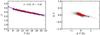 |
Fig. 5 As Fig. 4 but for HM(S), the hierarchical model using Student probability distributions. |
| In the text | |
|
Fig. 6 Comparison of the errors in the recovered parameters A (left-hand frames) and B (right-hand frames) of the β(T) relation. The observations consist of measurements at 100, 160, 250, 350, and 500 μm, with a relative noise of 5%. The true value of B is indicated in the frames. |
| In the text | |
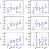 |
Fig. 7 As Fig. 6 but for a relative noise of 10%. |
| In the text | |
|
Fig. 8 As Fig. 6 but showing results for observations at 100, 350, 550, and 850 μm with a relative noise of 5%. |
| In the text | |
|
Fig. 9 As Fig. 8 (observations at 100, 350, 550, and 850 μm) but showing results for a relative noise of 10%. |
| In the text | |
|
Fig. 10 The accuracy of the parameters of the β(T) relation for sources in different temperature ranges. The results are based on measurements at 100, 160, 250, 350, and 500 μm with 5% relative noise and a β(T) relation with B = −0.3. The high and low temperature ranges correspond to temperatures above and below 14 K. The bottom frames show the results for the combined sample. |
| In the text | |
|
Fig. 11 The signal-to-noise ratio of the simulated observations of Sect. 4.3 as a function of the source temperature. The left-hand frame corresponds to the simulated Herschel observations at 100 μm (solid line), 160 μm (dashed line), 250 μm (dash-dotted line), and 500 μm (dotted line). The right-hand frame shows the signal-to-noise ratios for the simulated IRAS 100 μm data (solid line) and the Planck 500 μm and 850 μm bands (dashed and dotted lines, respectively). The signal-to-noise ratio of the 350 μm observations is 40. The black lines correspond to the relation β = 2.2(T/20.0)-0.3 and the red lines to β = 2.2(T/20.0)+ 0.3. |
| In the text | |
|
Fig. 12 The errors of the parameters of the β(T) relation in case of Herschel observations with fixed absolute noise levels. |
| In the text | |
|
Fig. 13 The errors of the parameters of the β(T) relation in the case of IRAS and Planck observations with fixed absolute noise levels. |
| In the text | |
|
Fig. 14 Comparison of the errors in the A and B parameters of the β(T) relation, comparing cases with 50 or 500 observed sources. The methods of analysis are χ2, SIMEX, BM, MC, and HM(S). For each method, two boxplots are shown, the 50-source case on the left and the 500-source case on the right. The observations consist of data in Herschel bands at wavelengths 100–500 μm and with a relative noise of 10%. |
| In the text | |
|
Fig. 15 Comparison of the errors in the A and B parameters of the β(T) relation, comparing cases where the source temperatures follow a uniform (U) or a normal (N) distribution. The compared methods of analysis are BM, HM(N), and HM(S). The observations consist of data in Herschel bands at wavelengths 100–500 μm and with a relative noise of 10%. |
| In the text | |
|
Fig. 16 The 250 μm surface brightness, dust colour temperature, and spectral index maps for the MHD model cloud. The values correspond to the χ2 solution with noiseless data. |
| In the text | |
|
Fig. 17 The distributions of (T, β) values for different methods (χ2, BM, HM(N), and HMC) and for the MHD model and noise levels N = 0.0–0.5. The values are the Bayesian estimates of the individual pixels.To guide the eye, a single contour following the solution for the N = 0.0 case is plotted in each frame. The colour scale corresponds to logarithmic number of pixels per a (T, β) interval. |
| In the text | |
|
Fig. 18 The parameters estimated from noisy data versus the true values obtained from noiseless observations. The upper frames correspond to the BM method and the lower frames to the HM method. In each frame, black and red points correspond, respectively, to the noise levels of N = 0.1 and N = 0.2. |
| In the text | |
|
Fig. 19 Distribution of recovered Tand β values for MHD model with noise N = 0.1 and the HM method with probabilities being calculated either with normal distribution (left-hand frame) or with Student distribution (right-hand frame). The colour scale corresponds to logarithmic number of pixels per (T, β) interval. |
| In the text | |
|
Fig. 20 Deviations from the fitted modified black body law in the case of the MHD model. The plot shows the relative deviations for 5% of the highest (blue symbols) and 5% of the lowest column density (black symbols with larger error bars) pixels. The error bars correspond to noise per pixel for the general noise level N = 0.1. The dotted line shows relative deviations between a ν2.1 dependence and the actual opacity in the employed dust model. |
| In the text | |
|
Fig. 21 The distributions of (T, β) values for data containing calibration errors where either 160 μm data (first six frames) or the 350 μm data (six last frames) has been scaled by 1.1. The methods are χ2, BM, HM, and HMC, the last one corresponding to a hierarchical model that includes free parameters for multiplicative corrections in three bands. Each frame corresponds to one combination of method and statistical noise, as indicated in the frames. The single contour corresponds to the locus of the correct solution (see Fig. 17). |
| In the text | |
|
Fig. 22 The 160 μm (frame a)) and 350 μm (frame b)) surface brightness maps (N = 0.1) that include stripes with constant surface brightness offsets. The white lines indicate the widths of these stripes. Frames c) and d) show the distribution of (T, β) values obtained with HM for all the pixels (frame c)) and separately for the pixels outside the stripes (frame d)). Frames e) and f) show the corresponding results for method HMC. The black contours correspond to the distribution of values for method HM, in the case of no stripe artefacts and no noise (see Fig. 17). In frames c–f), the colour scale corresponds to logarithmic density of pixels per a (T, β) interval. |
| In the text | |
|
Fig. 23 Results for the Herschel field G109.80+2.70. The upper frames show the observed 250 μm surface brightness and the temperature and spectral index maps from the χ2 method. The lower frames show the distributions of the (T, β) values obtained with the χ2, BM, and HM(N) methods, the colour scale corresponding to logarithmic number of pixels per (T, β) interval. The solid lines are least square fits with the parameters A and B given at the bottom of each frame. |
| In the text | |
|
Fig. 24 The residuals between the observed 160 μm surface brightness in the field G109.80+2.70 and the χ2 fit. The residuals are shown both as absolute errors (left frame) and relative to the χ2 fit. |
| In the text | |
|
Fig. 25 The (T, β) distributions of the field G109.80+2.70 from hierarchical models that include multiplicative calibration factors (left frame) or zero point offsets (right frame) as additional parameters. |
| In the text | |
|
Fig. 26 Comparison of results of different versions of the hierarchical methods, HM(N), HM(S), and HM(SL) where the last one fits the intensity and temperature on a logarithmic rather than at a linear scale. The observations consist of Herschel wavelengths with the absolute errors as described in Sect. 4.3. |
| In the text | |
|
Fig. 27 Comparison of the derived (T, β) values in the case of simulated modified black body spectra of different noise level (cf. Sect. 4). The black solid lines correspond to the relation assumed in the simulation of the observations. The measurements have 5% or 10% relative errors or the absolute errors described in Sect. 4.3. In the fourth column of frames, the observations follow two distinct β(T) relations (black solid lines) with 20% relative errors for the low temperature branch (T < 15 K) and 5% relative errors for the high temperature branch (T > 14 K). The left-hand frames show some MCMC samples (coloured dots), their averages (red circles) and the fitted β(T) relations (dashed blue lines). The right hand frames show the distributions for the errors ΔT and Δβ. The plots correspond to a single noise realisation of observations of 50 sources. |
| In the text | |
Current usage metrics show cumulative count of Article Views (full-text article views including HTML views, PDF and ePub downloads, according to the available data) and Abstracts Views on Vision4Press platform.
Data correspond to usage on the plateform after 2015. The current usage metrics is available 48-96 hours after online publication and is updated daily on week days.
Initial download of the metrics may take a while.