| Issue |
A&A
Volume 551, March 2013
|
|
|---|---|---|
| Article Number | A18 | |
| Number of page(s) | 31 | |
| Section | Galactic structure, stellar clusters and populations | |
| DOI | https://doi.org/10.1051/0004-6361/201219994 | |
| Published online | 12 February 2013 | |
Near-infrared proper motions and spectroscopy of infrared excess sources at the Galactic center⋆
1
I. Physikalisches Institut, Universität zu Köln,
Zülpicher Str. 77,
50937
Köln,
Germany
2
Max-Planck-Institut für Radioastronomie,
Auf dem Hügel 69,
53121
Bonn,
Germany
e-mail: This email address is being protected from spambots. You need JavaScript enabled to view it.
3
European Southern Observatory, Alonso de Cordova 3107, Vitacura, Casilla 19,
19001
Santiago,
Chile
4
Astronomical Institute, Academy of Sciences,
Bocni II 1401,
14131
Prague, Czech
Republic
5
Université de Toulouse, UPS-OMP, IRAP, 31400
Toulouse,
France
6
CNRS, IRAP, 14
avenue Édouard Belin, 31400
Toulouse,
France
Received:
12
July
2012
Accepted:
23
November
2012
Abstract
Context. There are a number of faint compact infrared excess sources in the central stellar cluster of the Milky Way. Their nature and origin is unclear. In addition to several isolated objects of this kind there is a small but dense cluster of comoving sources (IRS13N) located ~3′′ west of SgrA* just 0.5′′ north of the bright IRS13E cluster of Wolf-Rayet and O-type stars. Based on the analysis of their color and brightness, there are two main possibilities: (1) they may be dust-embedded stars older than a few Myr; or (2) very young, dusty stars with ages younger than 1 Myr.
Aims. We present a first Ks-band identification and proper motions of the IRS13N members, the high-velocity dusty S-cluster object (DSO, also referred to as G2), and other infrared excess sources in the central field. Goal is to constrain the nature of these source.
Methods. The L′- (3.8 μm) Ks- (2.2 μm) and H-band (1.65 μm) observations were carried out using the NACO adaptive optics system at the ESO VLT. Proper motions were obtained by linear fitting of the stellar positions extracted by StarFinder as a function of time, weighted by positional uncertainties, and by Gaussian fitting from high-pass filtered and deconvolved images. We also present results of near-infrared (NIR) H- and Ks-band ESO-SINFONI integral field spectroscopy of the Galactic center cluster ISR13N.
Results. We show that within the uncertainties, the positions and proper motions of the IRS13N sources in Ks- and L′-band are identical. The HK−sL′ colors then indicate that the bright L′-band IRS13N sources are indeed dust-enshrouded stars rather than core-less dust clouds. The proper motions also show that the IRS13N sources are not strongly gravitationally bound to each other. Combined with their NIR colors, this implies that they have been formed recently. For the DSO we obtain proper motions and a Ks-L′-color.
Conclusions. Most of the compact L′-band excess emission sources have a compact H- or Ks-band counterpart and therefore are likely stars with dust shells or disks. Our new results and orbital analysis from our previous work favor the hypothesis that the infrared excess IRS13N members and other dusty sources close to SgrA* are young dusty stars and that star formation at the Galactic center (GC) is a continuously ongoing process. For the DSO the color information indicates that it may be a dust cloud or a dust-embedded star.
Key words: Galaxy: center / stars: early-type / infrared: stars
Appendix A is available in electronic form at http://www.aanda.org
© ESO, 2013
1. Introduction
The formation of young and massive stars is an important process at the center of the Milky Way (see e.g. Paumard et al. 2006; Ghez et al. 2005). In the central half parsec of the Milky Way these objects are organized in at least one disk-like structure of clockwise rotating stars (CWS; Genzel et al. 2003; Levin & Beloborodov 2003; Paumard et al. 2006) and the existence of a second, less populated disk of counter-clockwise rotating stars (CCWS) has been proposed by Paumard et al. (2006). It is unclear how these young stars have been formed in the strong tidal field of the super-massive black hole (SMBH) at the position of SgrA*. There are two prominent scenarios: one includes star formation in-situ (in an accretion disk; Levin & Beloborodov 2003; Nayakshin et al. 2006), the other requires the in-spiral of a massive stellar cluster that formed at a safe distance of 5−30 pc from the Galactic center (Gerhard et al. 2001; McMillan & Portegies Zwart 2003; Kim et al. 2004; Portegies Zwart et al. 2006). Currently the in-situ scenario appears to be favored by a number of authors (Nayakshin & Sunyaev 2005; Nayakshin et al. 2006; Paumard et al. 2006). Also, results by Stolte et al. (2009, 2010) seem to rule out the possibility that known compact clusters close to the GC (such as the Arches cluster) could migrate inwards and fuel the young stellar population at the very center.
A prime object for testing these scenarios both observationally and theoretically is the IRS13 group of sources. IRS13E (located ~3′′ west and ~1.5′′ south of SgrA*) is the densest stellar association after the immediate vicinity of SgrA* and contains several massive Wolf-Rayet (WR) and O-type stars (Maillard et al. 2004; Moultaka et al. 2005; Paumard et al. 2006; Fritz et al. 2010). It is generally considered to be associated with the mini-spiral (Moultaka et al. 2005; Paumard et al. 2004). For IRS13E four out of seven identified stars show highly correlated velocities (Maillard et al. 2004; Schödel et al 2005), indicating that is probably bound. It is unclear what the origin of the IRS13E group of stars is. It is conceivable that such a cluster could have been formed in an accretion disk as described by Milosavljevic & Loeb (2004) and Nayakshin et al. (2005). However, numerical simulations have shown that it is difficult to explain the formation of such a dominant feature in a star-forming disk (Nayakshin et al. 2007). To support the cluster in-fall scenario, an intermediate-mass black hole (IMBH) was proposed to reside in the center of the cluster (Maillard et al. 2004). The existence of an IMBH results in a higher dynamical friction and a higher stability of the in-falling cluster such that this process in general is more efficient. It would allow compact clusters to reach the central parsec of the Galaxy (with >106 M⊙) within their lifetimes (Hansen & Milosavljevic 2003; Berukoff et al. 2006; Portegies Zwart et al. 2006; but see Kim et al. 2004 for a characterization of the problems with this hypothesis). However, the presence of the IMBH that would be required to stabilize IRS13E is highly disputed. Schödel et al. (2005) analyzed the velocity dispersion of cluster stars. The authors found that the mass of such an object should be ≥7000 M⊙. However, both the X-ray (Baganoff et al. 2003) and the radio (Zhao & Goss 1998) source at the position of IRS13E can be explained by colliding winds of high-mass-losing stars (Coker et al. 2002; Zhao & Goss 1998). These findings make the presence of an unusual and massive and dark object in IRS13E unnecessary.
In addition to the IRS13E association there are a number of faint infrared excess sources that may be essential for the discussion of star formation in the central stellar cluster (see Eckart et al. 2006; Perger et al. 2008). In some cases there is spectroscopic evidence for them being associated with young stars (Perger et al. 2008). Here we present new proper motion and new spectroscopy data on these objects1. These comprise first Ks-band proper motion measurements of sources that include the IRS13N association, and several sources at a projected distance of only a few arcseconds from SgrA*.
Approximately 0.5′′ north of IRS13E, a small cluster of unusually red compact sources has been reported (IRS13N; Eckart et al. 2004). Muzic et al. (2008) gave a detailed analysis of this cluster and showed that an orbital analysis supports that the cluster is a comoving group of young stars. A strong infrared excess is due to the emission of warm dust (T ~ 1000 K; Moultaka et al. 2005). The authors proposed two possible explanations for the nature of IRS13N: (1) objects older than a few Myr and similar to bow-shock sources reported by Tanner et al. (2005); or (2) very young stars (0.1−1 Myr old). The latter scenario implies more recent star formation than has been assumed so far for the GC environment.
Recently, Gillessen et al. (2012a) reported a fast-moving strong infrared excess source, which they interpreted as a core-less gas- and dust cloud approaching SgrA*. Owing to its location and because it is apparently on an elliptical orbit around SgrA*, we refer to it in the following as the dusty S-cluster object (DSO). The community has started to call the newly found fast-moving object G2 (e.g. Burkert et al. 2012), reminiscent of the gas cloud G1 found by Clenet et al. (2005). As we show in the present paper, it cannot be excluded that the newly found object is instead a star with a gas/dust shell or disk around it, and not a core-less gas cloud as claimed by Gillessen et al. (2012a). We therefore propose to call it DSO rather than G2 since the acronym DSO (Dusty S-cluster object) reflects the true nature of the source in a more realistic way. While essential properties of this source have already been described by Gillessen et al. (2012a), no continuum identification of it shortward of 3.5 μm has been published to date. In other cases of near-infrared (NIR) excess sources (e.g. see Fig. 14 in Eckart et al. 2006) a detailed investigation of their nature had not yet been carried out. We also present first Ks-band proper motion studies of the DSO.
After the introduction we describe the observations and data reduction in Sect. 2. In the results Sect. 3 we derive the proper motions and then outline the physical properties of the sources in Sect. 4. In Sect. 5 we give a summary and the appendix contains additional maps and graphs.
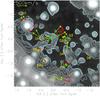 |
Fig. 1 Proper motion vectors of dusty objects in the central stellar cluster of the Milky Way (see Table 4). We show the May 10, 2003, adaptive optics L′-band image of the central 4′′ × 4′′. The arrows indicate the uncertainties in amount (red or yellow portion of the otherwise green arrow) and angle of the measured proper motion derived from data between 2002 and 2008 in the H, Ks, and L′-bands (see Table 1). |
2. Observations and data reduction
2.1. NACO near-infrared imaging
The imaging data in the H-, Ks-, and L′-bands were obtained with the NAOS/CONICA adaptive optics (AO) assisted imager/spectrometer (Lenzen et al. 1998; Rousset et al. 1998; Brandner 2002) at the UT4 (Yepun) at the ESO Very Large Telescope (VLT). IRS7, a supergiant with Ks ≈ 6.5−7.0 mag and located ~5.5′′ north from SgrA*, was used to lock the AO loop using the NIR wavefront sensor. We used data whose observing dates and pixel scales for the sources in the central few arcseconds, the IRS13N sources and the DSO are given in Table 1. Data reduction was standard, with sky subtraction, bad-pixel correction, and flat-fielding. Randomly dithered exposures were median-averaged to obtain final mosaics. The sky background in the H- and Ks-band was measured on a dark cloud about 400′′ north and 713′′ east of the GC. In the L′-band, the sky background was extracted from a median of the dithered science exposures. These are images in which the profiles of single stars are sharply peaked and have no broad wings. In the Ks-band one can see a diffraction-limited stellar image (in some cases with an indication of a diffraction ring) on top of a more extended foot that stems from the residual of the AO seeing correction. From these images we selected data sets in which the NIR PSF close to SgrA* has a FWHM of less that 0.25′′ (estimated through the second-order moment; optical guide star seeing typically <0.5′′) and an estimated FWHM of the diffraction limited part of the PSF of better than 1.5 times the diffraction limit (by visual inspection of the PSF profiles). The diffraction-limited FWHM values in the H-, Ks-, and L′-band are about 42 mas, 56 mas, and 98 mas (NaCo instrument manual). Infrared PSF width estimates for all NACO H-band data until 2008 are given with the light curves by Bremer et al. (2011). Active optics guide star PSF width estimates obtained in the optical for all NACO Ks-band data until 2010 are given in Fig. 20 by Witzel et al. (2012). For the years 2002 and 2009−2012 we did not find high-quality H-band imaging VLT data. The work of Bremer et al. (2011) and Witzel et al. (2012) as well as the comparison to published data suggests that the flux densities and colors of the sources we investigated are constant to within 40% and 80%.
The sources in the wider field of the central star cluster are shown in Fig. 1. The IRS13E and IRS13N clusters are shown in Figs. 2 and 3. The relative and absolute coordinates of the lower left (southeastern) corner of the images are listed in Table 2. In the IRS13N region eight sources were resolved and labeled α through κ, as shown in Figs. 4−7. The nomenclature is taken from Eckart et al. (2004).
2.2. SINFONI imaging spectroscopy
Spectroscopy of the region around IRS13 was carried out in June 2009 using SINFONI, the AO-assisted integral field spectrometer mounted at Yepun, Unit Telescope 4 of the ESO VLT in Chile (Eisenhauer et al. 2003). The AO guiding was carried out in the optical using an R ~ 13.9 star located ~19′′ from SgrA*. We used the Ks-band grating, which provides spectral resolution of 4000; the spatial setting of 0.1′′ per image slice results in a field-of-view of 3′′ × 3′′. The mean Strehl ratio of the cube (measured from Brγ) is about 7%. The sky was sampled on the same dark cloud as in the case of NACO observations, and the total on-source time was 14 × 300 s. Because of the non-quadratic shape of the SINFONI pixels (50 mas × 100 mas), the observations were split into two blocks observed at position angles of 0 and 90 degrees. The two cubes were combined into a single data cube as a final step in the reduction procedure. To combine the two data cubes, we first de-rotated the second cube by 90 degrees to match the orientation of the first one. Both data cubes were re-binned to a unique pixel scale of 50 mas × 50 mas using the IDL task “congrid” and were median-collapsed. The resulting images were then cross-correlated to determine the offsets that can be supplied to the pipeline recipe “sinfo_utl_cube_combine”. The recipe shifts the two cubes and co-adds them to produce the final data cube.
The 3D cubes were reduced and reconstructed with the ESO-supported SINFONI reduction software package. Bad pixel, cosmic rays, and flat-field corrections were applied to the 2D raw frames. The 3D cubes were reconstructed using calibration frames for the slit-let distances and the light dispersion. Intermediate standard-star observations of a nearby G2V star were used to correct for strong atmospheric (telluric) absorptions. The standard-stars were observed near in time and airmass to the target exposures. The G2V spectral characteristics were removed by dividing the standard-star spectrum by the well-known, high signal-to-noise solar spectrum (NSO/Kitt Peak spectra, as provided at the ISAAC/VLT web page).
The flux was calibrated with the known fluxes of the IRS13N cluster sources (Eckart et al. 2004; Muzic et al. 2008), since we are primarily interested in measuring line ratios. The total flux within the SINFONI FOV was scaled according to these values. The positional registration of the data cube was performed via the know positions of the bright IRS13E sources and its uncertainty is about 0.05′′.
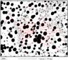 |
Fig. 2 High-pass-filtered image of the IRS13E/IRS13N field in the Ks-band. The labels correspond to those in Table 3. Source 1 to 6 are sources E1 to E6 in IRS13E. The angular resolution is close to the diffraction limit of 60 mas. |
Relative and absolute coordinates of the lower left (southeastern) corner of the image sections shown in the corresponding figure.
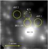 |
Fig. 3 Wavelength-integrated 2 μm SINFONI data cube. Yellow circles mark the regions in which the spectra were obtained. The angular resolution is about 0.11 arcsec. |
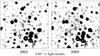 |
Fig. 4 Ks-band identification of individual IRS13E and IRS13N sources at two different epochs and visualizations of the positions of the IRS13N sources α, β, δ, ϵ, η, and κ at two different epochs. The source labels in the high-pass filtered images correspond to those in Table 3. |
From the final reconstructed 3D cube we extracted spectra and emission line maps. In Figs. 8 and 9 we show the K- (intermediate continuum band IB 2.15 μm) and L′-band (3.8 μm) images with the Brγ and [FeIII]-emission lines and the CO absorption line maps in contours overplotted. The contours in Figs. 8−10 are labeled with percentages of the peak flux. The emission line maps presented in Fig. 8 were created by summing the flux of the emission line and then subtracting the average flux density of the continuum to the left and right of the line. The wavelength ranges we used for the maps are Brγ: 2.16−2.17 μm; [FeIII] (2.242 μm): 2.2395−2.2438 μm; [FeIII] (2.3479 μm): 2.3460−2.3515 μm; [FeIII] (2.2178 μm): 2.2154−2.2197 μm; CO-absorption: 2.2932−2.3015 μm. These wavelength ranges are several times larger than a typical radial velocity offset. This is true both for the stellar sources and the extended emission in the observed region, because the absolute values of the radial velocity do not exceed 150 km s-1 (Paumard et al. 2004, 2006; Zhao et al. 2009). The absorption line maps presented in Fig. 9 were created by extrapolating the continuum shortward of 2.29 μm and subtracting it from the measured spectrum. The maps were then produced by plotting the negative value of the line integral over the strongest CO-bandhead between 2.290 μm and 2.300 μm.
In Fig. 10 we show the radio image from Zhao et al. (2009) with line maps in contours overplotted. The radio data and our imaging field spectroscopy data cubes were essentially taken at the same epoch. In addition, we extracted spectra for specific regions as shown in Fig. 3. The radius of the extraction regions is 5 pixels (0.25′′). In Fig. 11 we show the integrated Ks-band spectrum of IRS13N and for comparison the spectra of the nearby regions east and west of IRS13N that are dominated by diffuse emission. the integrated Ks-band spectrum of the [FeIII]-emission line blob north of IRS13 N is presented in Fig. 12. As indicated by the shape of the [FeIII] line at 2.3479 μm, this line might be a blend with the weaker HeII line that is close in wavelength.
3. Results
3.1. Deriving the proper motions
At a distance of 8 kpc the GC is well-suited to derive proper motions of stars (Eckart & Genzel 1996; Ghez et al. 2000; Eckart et al. 2002) and dusty filaments (Muzic et al. 2007). In the framework of the GC, proper motions have mostly been used to derive a mass estimate of the potential the stars are moving in (e.g. Schödel et al. 2009; 2005; Ghez et al. 2005) or to explore the origin and dynamics of young and old stellar populations in the central cluster (e.g. Genzel et al. 2003; Levin & Beloborodov 2003; Ghez et al. 2005; Paumard et al. 2006; Schödel et al. 2005, 2009 Muzic et al. 2008; Bartko et al. 2010; Lu et al. 2008). However, comparing the proper motions is also a unique tool to identify sources across different wavelength bands. In this paper we use this technique to identify stellar counterparts of dusty sources in the GC stellar cluster. No correction for image distortions was applied. However, the comparison to published positions and proper motions shows that the linear and quadratic distorions across the small (≪ 5′′) fields that we considered are less than 5 × 10⁻⁴ and 5 × 10⁻⁵. The small corrections for image rotation that we applied are less then 3 × 10⁻² degrees. Details are given in the following subsections.
 |
Fig. 6 Visualization of the Ks-band identifications of the IRS13N sources γ, δ, ϵ, and ζ at four different epochs in high-pass filtered images. The source labels correspond to those in Table 3. |
3.1.1. Proper motions of IRS13N and IRS13E
To derive the Ks-band proper motions of the IRS13N cluster sources it is necessary to work on images with a very high point source sensitivity for each epoch. In each epoch the faint Ks-band counterparts of the significantly brighter L′-band sources had to be identified. A first identification for epoch 2002 was given by Eckart et al. (2004). The Ks-band sources are faint compared to the IRS13E sources and deconvolution or point spread function (PSF) fitting is not sufficient to provide source identifications for all epochs. Therefore, we produced high-pass filtered images of the highest Strehl Ks-band images. In these images the peak of the diffraction-limited core of the AO images is highlighted and the surrounding emission is strongly suppressed.
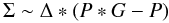
The high-pass filtered image can be produced by calculating a smooth-subtracted image Σ
as  (1)The symbol ∗ denotes
the convolution operator, Δ denotes the distribution of stellar sources, and
E represents the distribution of extended emission. Here
P is the PSF and I the image that results from the
convolution of P and the object distribution
O = Δ + E. We used a narrow Gaussian
G normalized to an integral power of unity. It is our experience that
it is best to choose the Gaussian G to have a width that corresponds to
about 30% to 50% of the full width at half maximum of a diffraction-limited core of a
stellar AO image. The smooth-subtracted image can then be rewritten as
(1)The symbol ∗ denotes
the convolution operator, Δ denotes the distribution of stellar sources, and
E represents the distribution of extended emission. Here
P is the PSF and I the image that results from the
convolution of P and the object distribution
O = Δ + E. We used a narrow Gaussian
G normalized to an integral power of unity. It is our experience that
it is best to choose the Gaussian G to have a width that corresponds to
about 30% to 50% of the full width at half maximum of a diffraction-limited core of a
stellar AO image. The smooth-subtracted image can then be rewritten as
 (2)Since the width of the
extended emission is much larger than the width of the PSF (for the one-dimensional (1D)
case see discussion on narrow dust features by Muzic et al. 2007), we can then infer that
E ∗ P ∗ G ~ E ∗ P
and the high-pass filtered differential image is
(2)Since the width of the
extended emission is much larger than the width of the PSF (for the one-dimensional (1D)
case see discussion on narrow dust features by Muzic et al. 2007), we can then infer that
E ∗ P ∗ G ~ E ∗ P
and the high-pass filtered differential image is
 (3)(see also Sabha
et al. 2010). If the image is clipped at zero
flux, density the remainder of
P ∗ G − P represents the top
section of the diffraction-limited PSF core of the AO image and Σ is an approximation of
an image of the point sources in the field. To give a higher weight to signals close to
and below the spatial frequency of the PSF we convolved the high-pass-filtered image
again with the Gaussian G.
(3)(see also Sabha
et al. 2010). If the image is clipped at zero
flux, density the remainder of
P ∗ G − P represents the top
section of the diffraction-limited PSF core of the AO image and Σ is an approximation of
an image of the point sources in the field. To give a higher weight to signals close to
and below the spatial frequency of the PSF we convolved the high-pass-filtered image
again with the Gaussian G.
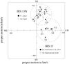 |
Fig. 7 Comparison of Ks- and L′-band proper motions in right ascension and declination for the GC IRS13E and the IRS13N cluster (indicated by circles in dashed lines). The direction of the motion, i.e., S to N, or E to W, is labeled. The source labels correspond to those in Table 3. The Ks-band motions derived here are labeled with open dots. For IRS13 and for IRS13N the filled dots indicate the proper motions published by Fritz et al. (2010) and Muzic et al. (2008). The open circles depict the Ks-band proper motions described here. |
This high-pass filtering method has the advantage that no estimate of the PSF is required. The PSF is typically variable across the imaging field and has a finite size. The corresponding apodization radius and residuals from stars that have to be removed from the PSF wings (via a median procedure or explicit subtraction) are usually the cause for additional artifacts that spoil the image quality if high sensitivity is required. In addition, a deconvolution may suffer from small number division problems at high spatial frequencies, or it runs with a limited number of iterations, or a loop gain and a stopping or convergence criterion. A limited number of sources needs to be identified for PSF fitting. All these restrictions and their potential drawbacks do not have to be considered for the high-pass filtering method. The noise property of the high-pass filtering is intimately linked to the original noise in the image. All noise contributions with spatial frequencies significantly lower than the characteristic cutoff frequency of the filter (i.e. given by the FWHM of the Gaussian kernel) are strongly suppressed by subtracting the flux-conserved image from the original. Only the (already existing) image power around and above the characteristic cutoff frequency of the filter will remain. This includes power at the diffraction limit. Hence, there is no mechanism over which additional and spurious noise peaks can be introduced by the filtering process. high-pass filtering has, however, the disadvantage that PSF imperfections at high spatial frequencies, which may be introduced by the combined imaging optics (residual astigmatism, trefoil, etc.) are not corrected for.
Ks-band positions in arcseconds relative to SgrA* and proper motions in km s-1 of IRS13E and IRS13N sources at epoch 2005.83.
We derived the positions of individual sources in the high-pass filtered images from (1) Gauss-fits to the resulting source profiles and (2) by determining the peak position on a sub-pixel level. Within the uncertainties (see below) both methods resulted in the same proper motion values. To provide an accurate relative positional reference system the low proper motion stars 26−33 identified in Fig. 2 and the May 2005 positions of stars E1 through E6 in the IRS13E cluster (Fritz et al. 2010) were used to establish a calibrated reference frame that allowed us to compare the positions and proper motions to values in the literature: in particular Fritz et al. (2010) mainly for the IRS13E sources in Ks-band, Muzic et al. (2008) for the IRS13E and IRS13N sources in L′-band, and Schödel et al. (2005) for the IRS13E sources and stars in the wider 3′′ diameter field around the cluster obtained in the Ks-band.
The proper motions of sources α through κ can be inspected in Figs. 4−6. For demonstration purposes the pixel scale of 27 mas has been decreased (by interpolation) by a factor of 8. Gray scales have been adapted to the quality of the frame. Sources may in addition be influenced by blends with nearby background sources. In Table 3 we present the source name (Col. 1), a reference (2), a source identification (3), coordinates relative to SgrA* and the corresponding uncertainties (4−7), and proper motion values and the uncertainties (8−11). The uncertainties for the positions and proper motion values were derived from the linear regression fit to the positions at all epochs.
In Fig. 7 we compare the proper motion values of IRS13E and IRS13N sources obtained in L′-band (Muzic et al. 2008) to those obtained here in Ks-band. We compared our proper motion results with published values and quote the root mean square deviations in right ascension σRA and declination σDec.
These values have to be compared to the expected 1D proper motion velocity dispersion value of about 200 km s-1 at the location of the IRS13E and IRS13N clusters (Schödel et al. 2009).
The IRS13E sources E1 to E6 we agree well with the results of Fritz et al. (2010) σRA = 11 km s-1 and σDec = 22 km s-1 and with in comparison to the L′-band proper motion by Muzic et al. (2008) with σRA = 38 km s-1 and σDec = 44 km s-1. We regard the difference to Fritz et al. (2010) as a measure of our measurement uncertainty for bright sources in the Ks-band and the differences to Muzic et al. (2008) as a measure of the combination of our measurement uncertainties in the Ks-band and the corresponding L′-band uncertainties. The deviations from Schödel et al. (2005) are larger with σRA = 96 km s-1 and σDec = 77 km s-1, but here the baseline in time used to derive the motions was only three years. For the IRS13N sources β to η we compared our Ks-band proper motions to the L′-band values by Muzic et al. (2008) and found σRA = 65 km s-1 and σDec = 95 km s-1. Correcting for the uncertainties derived for bright sources from the comparison to the data by Muzic et al. (2008), we obtain a residual uncertainty value between the Ks-band and L′-band proper motions of σIRS13N, RA = 52 km s-1 and σIRS13N, Dec = 84 km s-1 that can be solely attributed to the faint co-moving IRS13N sources β to η (see Sect. 4).
3.1.2. Proper motions of the DSO
In the central arcsecond the source density is highest in the overall cluster. In this region we need the highest angular resolution in addition to high point source sensitivity to separate the faint and bright stars from each other and to search for a stellar counterpart of the dusty high-velocity S-star cluster source reported by Gillessen et al. (2012a). In addition to the high pass-filtering we therefore employed Lucy- and linear Wiener filtering. A detailed comparison of these with two algorithms with the CLEAN algorithm, which is sensitive to structures that are favored by high-pass filtering, is given in Ott et al. (1999). In the Ks-band we used the same images as for IRS13N. In the H-band we used the images employed for the HK-spectral index analysis of SgrA* presented by Bremer et al. (2011) that covers the years 2003 till 2008. In both bands we investigated the images at the derived L′-band positions of the dusty S-cluster object relative to the corresponding positions of the star S2 and SgrA*.
In addition, we compared the data with detailed simulations of the field including important, neighboring sources such as S23, S54, and S63. For these sources the proper motions, and in the case of S23 the curvatures, are listed in Table 9 by Gillessen et al. (2009). From S63 we derived the proper motions from our H- and Ks-band data, since the values listed by Gillessen et al. (2009) indicated a motion almost perpendicular to what we found. Our simulations clearly show that the DSO and star S63 blend each other from 2002 until 2007. In 2007 the DSO starts to emerge from the S63 PSF and is clearly distinguishable from the neighboring stars.
This results in Ks-band identifications for all epochs since 2007. We can use the 2008 H-band data to derive a lower limit for the DSO magnitude. Taking the background from the neighboring stars and the 3σ variation across the diffraction limited beam into account, we find a limit of mH > 21.2. See Figs. A.1−A.4. In Fig. 14 we show the proper motion of the DSO projected onto the sky compared to the orbital solution given by Gillessen et al. (2012a).
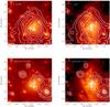 |
Fig. 8 2 μm-band image (left; IB 2.15 μm) and L′-band image (right; 3.8 μm) with the Brγ emission (top) and CO absorption (bottom) line maps in contours overplotted. |
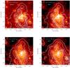 |
Fig. 9 2 μm-band image (left; IB 2.15 micron) and L′-band image (right; 3.8 μm) with [FeIII]-emission line maps in contours overplotted. |
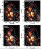 |
Fig. 10 13 mm VLA radio image from Zhao et al. (2009) with our Brγ- and [FeIII]-emission line maps in contours overplotted. |
3.1.3. Proper motions in the wider field of the central star cluster
The central parsec of the GC reveals different structures when observed at different wavelengths. In Fig. 14 shown by Eckart et al. (2006) these sources are denoted with D followed by a number. In Fig. 1 (taken on July 6, 2004 in the L′-band) we show the proper motions of some of these sources in the central few arcseconds (see also Fig. A.9 in the appendix). They are typically brighter than 14.6 in L′-band. Some of them appear to be circular symmetric on the sky (e.g. D2 and D5), others appear to be elongated (D3 and D4) or even filamentary, such as the source D8 at the eastern edge of Fig. 1 about −1.5′′ east and −0.5′′ south of SgrA*. The extended source D8 was excluded from our investigation since it is a very complex region in projection on the sky for which proper motions are difficult to obtain. Comparing Fig. 1 shown by Gillessen et al. (2009) to our Fig. 1, we can associate the position of the S-star S43 with the position of D2 (see also Table 4). Within the uncertainties both objects also compare well in their H-, Ks-, and L′-band proper motions. For sources D3, D5, and D7 we could only determine L′-band proper motions. For D4 the data are given by Muzic et al. (2010). For D2, D6, S90, F1, and F2 the Ks- and L′-band proper motions agree within the uncertainties given in Table 4.
The mosaics in L′-band were put into an astrometric frame (see Muzic et al. 2008). The H- and Ks-band data were transformed into the coordinate system of the Ks-band mosaic obtained on July 31, 2002, using the coordinate transformation procedure described by Muzic et al. (2008). The positions of the 30 reference stars are evenly distributed over the field and were determined using the IDL code STARFINDER (Diolaiti et al. 2000) for the coordinate transformation. The known proper motions were calculated from the reference stars positions taken from Schödel et al. (2009).
The peak positions of the objects were determined using two dimensional (2D) Gaussian fits in each mosaic and band. The uncertainties in the graphs are the 1σ uncertainty in the peak position and the uncertainties in velocities are the 1σ-uncertainty of the linear fits. Figure A.9 show detailed maps of the immediate environment of the infrared excess sources close to SgrA* in the central stellar cluster. Details of the proper motions are shown in Fig. A.10 and are listed in Tables A.1−A.3. As an overview the results are summarized in Table 4 and in Fig. 1. The figure shows that the motions in the different bands for each source can be related to each other, since the vectors point in the same direction within the error bars,
Names, positional offsets from SgrA* in arcseconds, proper motions in km s-1 of compact infrared excess sources in the central 2′′ field close to SgrA*.
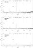 |
Fig. 11 Integrated Ks-band spectrum of IRS13N (top panel), spectrum of the nearby region Diffuse-1 west of IRS13N (middle panel) and Diffuse-2 east of IRS13N (bottom). The three spectra were normalized to the peak value of the Brγ line in the IRS13N spectrum. The spectra are continuum subtracted. |
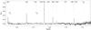 |
Fig. 12 Integrated Ks-band spectrum of the [FeIII]-emission line source at the position of source K21 (Zhao et al. 2009) north of IRS13 N. This spectrum is continuum subtracted normalized to the peak of the Brγ line. |
4. Discussion
4.1. Identification and proper motions of IRS13N sources
The derived stellar 1D velocity dispersion at that location is three times higher than the root mean square difference between the proper motions of the sources identified in the Ks and L′-band. In addition, the difference between our 2005.83 1D IRS13N source positions in the Ks-band and the L′-band positions by Muzic et al. (2008) at a mean epoch closer to 2005 is about 20 mas, i.e., two thirds of a Ks-band pixel of 27 mas size. This is on the same order (or below) of what is expected as the maximum change in position due to proper motions of the sources during the time difference between these mean epochs. We conclude that over the past 10 epochs we used to analyze the motion of the IRS13N sources the Ks-band sources can indeed be identified as being the co-moving counterparts of the L′-band sources. This also means that the L′-band sources are not unrelated (core-less) dust clouds as speculated by Fritz et al. (2010).
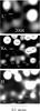 |
Fig. 13 Distinguishing the DSO against stars S57, S23, S54, and S63 in 2008 in L′- and Ks-band. Only an upper limit can be given in the H-band. |
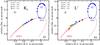 |
Fig. 14 Positions of the DSO relative to S2 and SgrA* plotted in comparison to the orbital tracks provided by Gillessen et al. (2012a) (red for the DSO, blue for S2, SgrA* is at the position of the black dot at the origin). The results for the Ks- and L′-band are shown in panels a) and b) (see data in Table 5). Thin lines indicate the approximate expected positions of the DSO on its orbit from 2002.0 to 2012.0 (based on our L′-band reductions and Gillessen et al. 2012a). The epochs are color-coded and the measurement uncertainty is shown as a black cross (see A.6 in the appendix). |
It is likely that not all sources α to κ that had been discussed in Eckart et al. (2004) belong to the same association. We pointed out already in Eckart et al. (2004) that κ has significantly bluer colors than the other IRS13N objects. Infdeed, it has not yet been identified with an L′-band source. Our Ks-band proper motion analysis also shows that it is moving south and west rather than predominantly north as all the other IRS13N members. From this we conclude that κ does not belong to the small IRS13N cluster of co-moving infrared excess sources.
Source α is farthest south of the Eckart et al. (2004) sources and has also a velocity offset from the other IRS13N sources. Here we give the L′-band velocities derived by Muzic et al. (2008) a higher weight, since in Ks-band the source is apparently located in a crowded region as well as in the wings of the bright IRS13E member E1. We conclude that α is also probably not a member of the small IRS13N cluster of co-moving sources. We are therefore left with the sources β to η that have been identified as co-moving and whose dynamics were analyzed in detail by Muzic et al. (2008).
Source η is significantly brighter in H-band than all other IRS13N sources. It also has a the highest velocity discrepancy between Ks and L′ with a difference of ~150 km s-1. If we assume that the IRS13N sources are embedded in their own dust disk or envelopes and that they all have a random orientation towards the observer, this implies an average opening angle of 180°/6 = 30° under which the source can be seen unobscured. From this one may conclude that the circum-stellar material almost entirely surrounds the objects. If the sources have disks, it means either that not all material has settled into the disk, or that these disks are as thick as they are long in diameter, or that they are significantly warped. All of this could be expected if the sources indeed belong to a dynamically young compact cluster of co-moving young stellar objects.
The velocity dispersions of sources β to η corrected for their measurements uncertainties is about 45 km s-1 for the L′-band data discussed by Muzic et al. (2008). For the less well determined motions derived from our Ks-band identifications this value is about a factor of 1.5 higher. The implications for the possibly associated stellar mass of the IRS13N association has been discussed in detail by Muzic et al. (2008). The result is that if the IRS13N cluster is gravitationally bound, these velocity dispersions imply a stellar mass that should be detectable. Hence, it is likely to be unstable, implying that the association and its members are (dynamically) young.
4.2. Nature of the IRS13N sources
In this paper we used the SINFONI line and continuum images for a qualitative interpretation of the nature of the extended and stellar sources only. A quantitative analysis of the line fluxes is beyond the scope of the paper and will be published elsewhere. The comparison between the Brγ line emission and the near-infrared continuum emission of the stars in the IRS13E/IRS13N field in Fig. 8 shows that the line emission peaks on one of the brightest components (E2) of IRS13E, covers the entire IRS13E cluster and extends to the IRS13N complex. The strength of the emission is correlated with the presence of stars in the field and is clearly not only associated with the stars, but comprises a diffuse component as well. The maps of the [FeIII]-emission depicted in Fig. 9 show that the line flux is peaked both on IRS13E (E2) and IRS13N. The [FeIII] flux also shows contributions from a diffuse component. In IRS13N the [FeIII] integrated line flux density peaks to within ≤ 0.1′′ close to sources ϵ and δ. Zhao et al. (2009) found a radio source labeled K23 that lies between ϵ and δ and has to within 3−4σ the same velocity as the mean velocity of the NIR counterparts of ϵ and δ.
Ks-, and L′-band positions of the DSO and the star S2 relative to the SgrA* position.
The integrated [FeIII] line emission is also peaked on a source about 0.15′′ north of η with offsets from SgrA* of −3.25′′ ± 0.03′′ in right ascension and −0.45′′ ± 0.03′′ in and declination. This position agrees with that of source K21 identified by Zhao et al. (2009) to within about 0.1′′. The authors found a proper motion velocity of vα = −224 ± 16 km s-1 and vδ = −421 ± 20 km s-1 toward the NNW. In the L′-band we do not find a clearly defined point source at the position of K21. The continuum flux density extension from IRS13N at that position is consistent with a source that is about a magnitude fainter (i.e. L′ ~ 12) than source η. At Ks-band no clear association to a source brighter than K ~ 16.3 can be established. This indicates that K21 is either associated with a stellar source even more reddened than the IRS13N sources or that the source K21 is a core-less dust source bright in [FeIII]-emission. The integrated line emission of Brγ is also extended and covers the position of K21. A spectrum of the infrared flux density at the position of K21 is shown in Fig. 12.
The comparison between the CO absorption and the near-infrared continuum emission in Fig. 8 shows that the IRS13N complex is clearly located at a minimum of the CO-absorption in the IRS13E/IRS13N field. The absorption is concentrated on a few stars in the field to objects about 0.5′′ east, west, and north of IRS13N. The minimum in the absorption strength centered on IRS13N comes close to the background value due to the overall central stellar cluster. Given the contribution through PSF wings of these stars at the location of IRS13N, this is fully consistent with the statement that most of the IRS13N sources (about 0.5′′ north of IRS13E) do not show any significant CO line absorption.
The comparison of the radio data by Zhao et al. (2009) (Fig. 10) shows that the radio continuum emission peaks to within ≤ 0.10′′ at the peaks or contour line excursions of the [FeIII] line emission. The radio continuum is more peaked on the IRS13E source E1. The correspondence to the [FeIII]-emission (in particular the 2.242 μm line emission) is best. The Brγ emission is clearly more extended than the bright radio continuum emission, highlighting that the radio emission is more dominated by the compact stellar sources than the more diffuse emission traced by Brγ.
The combined spectra on IRS13N and the two off-positions east and west (Figs. 3 and 11) demonstrate that the emission in the Brγ, H2 and in particular in the [FeIII] lines is brighter on IRS13E than in the off-positions. The spectra also demonstrate that the integrated CO-band head absorption toward IRS13E is as strong as toward the off-positions. This indicates that the CO-absorption at this position can be fully explained by the CO-absorption in the PSF wings of the bright nearby late-type stars and the overall stellar cluster background.
4.3. NIR colors and spectra of the IRS13N cluster
The analysis of the HK (i.e. a significant section of the SED) colors presented in Fig. 16 shows that they – if
dereddened – would not come to lie even close to the positions expected for colors of pure
dust-emitting sources but rather lie at the locations expected for objects that show a
mixture of stellar and dust emission (see also Eckart et al. 2004).
(i.e. a significant section of the SED) colors presented in Fig. 16 shows that they – if
dereddened – would not come to lie even close to the positions expected for colors of pure
dust-emitting sources but rather lie at the locations expected for objects that show a
mixture of stellar and dust emission (see also Eckart et al. 2004).
Compared to the immediate surroundings (except for the IRS13E cluster), the sources in the IRS13N region are clearly correlated with a minimum in CO absorption and an excess in Fe- and H-recombination line emission. While the excess in emission may in part be due to a local concentration of gas associated with the 13N association or possibly with the mini-spiral, the lack of CO absorption can be attributed to the predominantly early spectral type, as suggested from the NIR colors of the sources (Eckart et al. 2004).
While NIR CO absorption and emission is often present, it is not a necessary feature to be observed toward young massive stars. Out of 201 young massive stars in M17, Hoffmeister et al. (2006) found 30% to have featureless spectra. Half of those show an infrared excess that corresponds to basically the same percentage of the remaining 60% of the sources that show CO in absorption or emission. Almost a third of the featureless sources also tend to show X-ray emission and a fifth shows simultaneous infrared excess and X-ray emission.
Featureless sources have the tendency to be brighter in the NIR compared to other young stellar objects. From the distribution in Fig. 3 in Hoffmeister et al. (2006) we can conclude that featureless objects are typically up to two magnitudes more luminous compared to CO emission or absorption sources. They are apparently later than spectral class B3.
Compared to previous CO bandhead studies in star-forming regions, the investigation by Hoffmeister et al. (2006) is the most extensive and a fairly unbiased one. Casali & Eiroa (1996) argued that Class II sources tend to show CO absorption, while Class I sources are featureless. The thermal continuum emission from dusty in-falling envelopes can exceed the combined stellar and disk photospheric emission by almost an order of magnitude (Calvet et al. 1997; Hoffmeister et al. 2006). Hence, this process can result in featureless spectra. In addition, the veiling of an envelope will also weaken the CO absorption lines. The presence of envelopes with large-scale heights is consistent with the presence of a single bright source η in addition to five faint objects, as elaborated above. The presence of a disk, on the other hand, is likely to amplify the CO feature. Therefore, Hoffmeister et al. (2006) concluded that the 60 featureless objects in their sample of 201 sources in M17 are very likely Class I sources that have just started to build up an infrared excess that is progressively moving toward the mid-infrared (MIR) and NIR domain.
From model calculations Hoffmeister et al. (2006) infered that the observed CO absorption is most likely a sign of heavily accreting proto-stars. The mass accretion rates may be above 10-5 M⊙ yr-1. High accretion can be provided through angular momentum loss within a disk. We conclude that the absence of that feature may indicate that these stars are currently not strongly accreting or have not yet reached that phase. This would be the case if the luminosity of the in-falling envelope is strong against the emission from the disk.
We infer from the combination of the fact that the stellar sources are in a co-moving group (Muzic et al. 2008; Eckart et al. 2004) and the proper motions and the spectroscopy presented here (see below) that the IRS13N sources may be featureless young stellar objects, like Class I sources, in which a bright NIR disk has not yet been formed but in which the NIR/MIR excess is still dominated from surrounding and in-falling material.
4.4. Age of the IRS13N sources
Possible stellar identifications of the IRS13N sources have already been discussed extensively by Eckart et al. (2004) and Muzic et al. (2008). The fact that our data supports the finding that the sources (β to η; see below) are indeed co-moving poses serious problems to source identifications that involve stars with ages >3 Myr. Here we highlight a few more aspects concerning the identification of the sources with young stars:
Broad-band colors can give information on the nature of sources. In Fig. 16 (left) we compare the colors of dusty objects in the central few arcseconds of the Milky Way to the colors of young stellar objects as given by Hoffmeister et al. (2006). The sources of IRS13N are more highly extincted than the remaining dusty objects in the field. Their dereddened colors agree with those young dust enshrouded objects (details in Eckart et al. 2004). The assumption (see Sect. 4.3) that the IRS13N cluster members are Class I sources implies that they are young. In a recent study of stellar and circumstellar properties of six Class I proto-stars Prato et al. (2009) estimated their ages as <2 Myr. However, even the ages of young Class II/Class III sources are estimated to range between 0.1 and 1 Myr (Green & Meyer 1995; Luhman & Rieke 1999; see also van Kempen et al. 2009). This is consistent with the assumption of Eckart et al. (2004) that the IRS13N sources are good candidates for being YSOs or young Herbig Ae/Be stars with ages that may range between 0.1 and about ~3 Myr. Molinari et al. (2008) found that the time scales of the formation of stars are about 1−4 × 10⁵ years, with shorter times for higher masses (6 to 40 M⊙) (Hillenbrand et al. 1992; Fuente et al. 2002; Ishii et al. 1998). The orbital time scale for the combined motion of the entire IRS 13E/IRS13N complex and the mini-spiral gas of about 104 years (see also Muzic et al. 2008) is short compared to the plausible ages of the massive young stars. We also assume that their associated envelopes and disks can survive the hostile GC environment for at least 104 years (see discussion in Scally & Clarke 2001).
4.5. Broad-band spectrum of IRS13N
Inspection of the 1.2′′ angular resolution 1.3 mm map of the mini-spiral presented by Kunneriath et al. (2012a,b) shows that the IRS13N complex is associated with 1.3 mm continuum emission. Just north of IRS13E it shows itself as a compact source component with a flux density of 20 ± 3 mJy (see Fig. A.7). Arithmetically de-convolved with the beam, its size is less than 0.6 arcsec. In NE direction it is partially blended with IRS13E and a northern neighboring mm-source. In the 13 mm map presented by Zhao & Goss (1998; Fig. 3/PLATES therein) we can read off the map in their Fig. 3 an extended flux density of 11 ± 2 mJy with a compact source of about 3 mJy. These flux densities are consistent with a dominant nonthermal stellar wind contribution with an approximate mass load of 10-5 M⊙ yr-1 (e.g. Montes et al. 2009; Lang et al. 2005). This a mass load is typical for young luminous stars (Drake & Linsky 1989; Kudritzki et al. 1999; Crowther 2001).
Eckart et al. (2004) quoted H, Ks and L′ flux densities for individual IRS13N sources. Viehmann et al. (2005, 2006) gave NIR/MIR flux density values obtained in an ≈1′′ diameter circular aperture on IRS13N. In the J- and H-band and probably even in the Ks-band these 1′′ aperture flux densities are dominated by confusing fore- and background sources of the central cluster and the values by Viehmann et al. (2006) can probably only be taken as an upper limit. Due to the very red colors of the sources the 1′′ flux densities at longer wavelengths are most likely characteristic for the IRS13N sources. However, at these wavelengths dust emission becomes dominant. Our investigation of the Ks- and L′-band proper motions shows that the dust-emission-dominated L′-band flux densities can be fully associated with the stellar sources found at shorter wavelength. Hence, we assume that a dominant portion of the emission longward of the Ks-band can in fact be attributed to the IRS13N sources.
4.6. Proper motions and nature of the central dusty sources
Examination of the proper motions of the dusty sources in the central few arcseconds shows that 5 of the 10 L′-band excess sources identified in Eckart et al. (2004, see Fig. 1) have Ks-band counterparts. The color−color diagram in Fig. 16 (left) shows that the colors of dusty objects in the central few arcseconds of the Milky Way are bluer than those of the IRS13N sources. Correcting for the Galactic foreground extinction of approximately 27 mag in the visible places them at the location of the young stars discussed by Hoffmeister et al. (2006). The IRS13N sources are more highly extincted than the remaining dusty objects in the field. Correcting for the Galactic foreground extinction places them at the location of extincted young stellar objects in Fig. 16i (left). Sources β to η in IRS13N are therefore excellent candidates for being young stars with an average extinction around AV ~ 27.
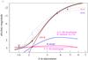 |
Fig. 15 Decomposition of the DSO spectrum including our Ks-band detection and H-band limit. Here we demonstrate that a mixture of dust and stellar contribution is possible. The points correspond to the L- and Ks-band magnitudes, and H-band upper limit from this work, and the M-band measurement and K-band upper limit of Gillessen et al. (2012a,b). Red and blue dashed curves also show their 550 K and 650 K warm dust fits. In solid blue, red, and magenta lines the emission from three different possible stellar types of the DSO core are plotted. Any of these stars embedded in 450 K dust (solid brown line) can produce the black line that fits all the NIR DSO photometric measurements. |
4.7. Pure dust versus photospheric emission
Here we investigate if the NIR emission of the infrared excess sources can be caused by pure dust sources or if significant contributions from photospherice emission of stars need to be included. If the objects were pure dust sources their observed colors must be consistent with reddened colors of pure dust sources. For the IRS13N this is apparently not the case. The DSO is clearly detected in the Ks-band at mK = 18.9. Using AK = 2.22 and approximating LK[L⊙] with 1.1 × 10⁴ × D [Mpc] 2 × SK [mJy] that results into SK = 0.13 mJy and LK [L⊙] = 92 × 10-3 L⊙. This is 46 times more than the luminosity in the Brγ line reported for the head of the DSO by Gillessen et al. (2012b). This implies that the 2 μm luminosity is dominated by the continuum rather than the Brγ line emission. In the H-band we find an upper limit mH > 21.2 if we consider the background level from the neighboxuring stars S23, S54i, and S63 in 2008, and the 3σ variation at the position of the DSO in the Ks- and L′-band. With the DSO L′-band brightness of mL′ = 14.4 ± 0.3 obtained from the observing epochs listed in Table 1 we obtain H − Ks = 2.3 as a lower limit (Fig. 16 right). This results in a measured color Ks − L′ = 4.5. With AH = 4.21, AKs = 2.22 and AL′ = 1.09, AM ~ AL′ (e.g. Viehmann et al. 2005; Lutz et al. 1996) the absolute magnitudes can be found and plotted in a spectrum (Fig. 15). In Fig. 16 (right) we compare the data to the black-body line and extincted colors of different mixtures between a stellar and a dust contribution (Glass & Moorwood 1985). The pure 550 K dust colors (Ks − L′ ~ 3.0) reddened by AV = 27 are consistent with the Ks − L′ color of the DSO. However (with the current H − Ks color limit and with potential H − Ks colors that range up to the pure 550 K color), the dereddened positions of the DSO show that the DSO colors are also consistent with a mixture between a stellar and a dust contribution. Withn its current (H − Ks color limited) position in the diagram, mixtures with 60% stellar emission and 40% dust with temperatures less than 550 K are possible. If the DSO will be detected half way between its current H − Ks and that of pure 550 K dust (striped circle in Fig. 16), 20% stellar and 80% 550 K dust contribution are possible. In Fig. 15 we show a possible spectral decomposition of the DSO using the M-band measurement by Gillessen et al. (2012a). In addition to their 550 K and 650 K fit and their mKs = 17.8 limit (dashed lines) we plot our Ks-band DSO detection and the H-band limit. The fit shows that the integrated flux can amount up to about 30 L⊙. We show a decomposition in which we assume that 50% of the current Ks band flux is due to a late dwarf (blue line) or an AF giant or AGB star (magenta line). We used dust at a temperature of 450 K plotted in red (see dereddening of the DSO in the color color diagram in Fig. 16 right). The sum of the spectra is shown by the thick black line (dashed at short wavelengths for the AF giant/AGB case).
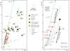 |
Fig. 16 Left: colors of dusty objects in the central parsec of the Milky Way compared to the colors of young stellar objects as given by Hoffmeister et al. (2006). The labels COAS and COES indicate that the sources show CO absorption or emission in their spectra. Right: colors of dusty objects in the central parsec of the Milky Way compared to colors of pure dust (temperatures given in red numbers) and mixtures of a stellar and a dust contribution (fractional numbers given in black; see also Glass & Moorwood 1985). Here we demonstrate that a mixture of dust and stellar contribution is possible. Because the H − Ks color of DSO is an upper limit, its NIR emission can be explained as pure dust at 550 K reddened by ~27 mag, or as a star embedded in warm dust, e.g., if its color were detected to be H − KS ~ 3.5 mag (dashed circle), after dereddening by 27 mag, its emission would be consistent with 20% stellar and 80% dust contributions. |
Similarly, after dereddening the IRS13N sources for AV = 27m, they miss the pure black-body line by about two magnitudes (see Fig. 16 left). For fully dereddened objects an offset of two magnitudes in Ks − L′ calls for temperatures of about 800 K or below with flux density contributions of a pure dust component of less than 50% (see also Fig. 7 by Glass & Moorwood 1985). This temperature estimate is consistent with the overall IRS13N temperature of around 650 K given by Fritz et al. (2010). This clearly implies that the IRS13N sources cannot be pure dust emitters but must have a stellar core. This is also fully consistent with the fact that the colors of these objects are similar to those of early dust enshrouded stars with colors shown the diagram in Fig. 16 (left). Hence, for IRS13N sources the evidence for photospheric emission from a star is strongly supported by the H-band detections (Eckart et al. 2004, Table 2 – here all sources except ϵ and γ could be identified).
Inspection of Fig. 16 (left), the black-body line shown in Fig. 16 (right) and comparison to Fig. 7 by Glass & Moorwood (1985) shows that within the uncertainties the sources F1 and D7 are good candidates for being pure dust sources. Sources D6 and S90 will have mostly stellar colors after dereddening with a possible contribution of dust >1000 K. Sources F2, D2, D3, D4, and D5 are clear candidates for being objects that show a mixture from photospheric emission and emission from dust with temperatures well below 1000 K.
4.8. Statistical robustness of the DSO identifications
Here we analyze the statistical robustness of the DSO identifications in the H- and Ks-bands. In Sabha et al. (2012) and Eckart et al. (2012) we tabulated the probability for finding a blend star above the confusion limit in a single Ks-band spatial resolution element in the overall region of the S-star cluster and at the position of SgrA*. With two independent methods we determined the central Ks-band confusion limit observationally. Sabha et al. (2010, 2012) employed successive subtraction of stars in the S-star cluster. Witzel et al. (2012) used the shape of the SgrA* flare amplitude histogram. The otherwise straight power spectrum with which this histogram can be described turns over at a flare flux density at which a mere flare detection becomes a flare flux density measurement (details in Witzel et al. 2012). This indicates a confusion limit in the range of 0.5 to 1.5 mJy.
The result of the statistical investigation of the S-star cluster by Sabha et al. (2012) is that for a range of observationally supported parameters that describe the structure and luminosity function of the cluster, the authors can give the probability of finding a blend star in a single spatial resolution element above the confusion limit. Here we use a power law index of the projected spatial distribution of α = 0.30 ± 0.05 and a K-band luminosity function exponent of KLF = 0.18 ± 0.07. Projecting the S-star cluster onto the sky blend stars are created by line of sight overlaps of fainter stars within a finite angular resolution element. The probability of finding blend stars in the central 1.3 × 1.3 arcsec2 overall can be as high as 1.0 and reaches a value of about 0.5 at the position of SgrA* itself. In the following we use these values although they can be much lower if the immediate vicinity of SgrA* is emptied of low-mass stars through stellar dynamical processes.
The probability of finding a Ks-band source in an L′-band resolution element (that corresponds to 2.8 Ks-band resolution elements) at a specific predicted position within the S-cluster is about 170 times lower than unity, i.e., 6 × 10⁻³. As explained in Sabha et al. (2012), the live time of these blend stars (also indicated through observations) is about 3 years during which they dissolve again into individual objects with flux densities below the confusion limit due to their proper motions. If one aims to explain the 2007−2012 Ks-band identifications of the DSO by blend stars, one requires about 2−3 of these transient apparent objects. This happens with a probability of 3 × 10⁻⁷. Since there is no guarantee that apparent proper motions during the dissolving phase of the blend stars follow the observed orbit and since we have chosen upper limits to start with, these low-probability values can be regarded as a safe upper limits for a scenario in which the DSO can be explained as the result of blend stars. Even if a blend star is assumed, one can think of at least 5−10 proper motion velocity values and 5−10 directions that would be expected given the accuracy of 13−25 mas and the involvement of 2 to 6 epochs. This will lower the probabilities quoted above by a factor of 25−100. This implies that the combined probability of being confused by a comoving blend star is less than 10-4.
However, the number of bright, single stars in the central region is high. We can therefore consider the likelihood of finding faint stars above the confusion limit at the position of the DSO over a time span of several years. From the KLF analysis by Sabha et al. (2010, 2012) we infer a maximum of about 40 stars fainter than 16 magnitudes (dereddened) within the central 1.3′′ × 1.3′′. This implies 0.2 sources per resolution element and observing epoch. For six consecutive epochs this results in a probability of about a percent to find a random configuration of the central cluster such that a faint star is found at consecutive positions given by the L′-band detections. If we include the immediate neighborhood (i.e., 9 to 25 surrounding resolution elements), the probability can rise to 25%. With a limited accuracy of determining the direction and value of the proper motion, this implies that the likelihood of finding a star that is close in position and velocity is in the percentage range. This may explain the confusion of the DSO with S63 in the interval 2002 to 2007.
In summary, the contamination with a bright field star over the entire time interval 2002 to 2012 is likely (around a few percent) but being confused by blend stars is very unlikely (≤ 10-4). For the IRS13N and all other infrared excess sources discussed here the projected stellar densities are even lower than those close to the center, such that serendipitous identifications are also not very likely.
4.9. Proper motions and identification of the DSO
The analysis presented here shows that the dusty S-cluster object reported by Gillessen et al. (2012a) does indeed have a Ks-band counterpart. Its H − Ks-color limits indicate that it cannot be excluded that the DSO is an embedded star rather than a pure dust cloud. Gillessen et al. (2012a) showed that both in proper motions and radial velocities the trajectory of the source perfectly fits a closed elliptical orbit. The authors interpreted this source as a dust cloud that is approaching SgrA* and will be disrupted during the peri-bothron passage. The combination of the fragility of the cloud and the fact that it is on a bound elliptical orbit implies that the object must have been on that orbit for a couple of revolutions. In the harsh environment of the central stellar cluster the evaporation time scale for a pure dust cloud is incompatible with this fact. The dust cloud would disappear before it can establish a relaxed orbit. If the object is on a bound orbit as a cloud and since it will be heavily stretched out by tidal forces during the peri-bothron passages it should not be as compact as it currently appears. Variations in the shape should (with lower angular resolution than in the H- and Ks-band) be traceable in the bright L′-band continuum where it appears to be rather compact (Gillessen et al. 2012a). In the Ks-band the DSO is close to the confusion limit (see discussion in Sect. 4.8). Given the strong and extended Brγ recombination line emission from the mini-spiral the situation may be similar for the DSO Brγ line emission. As in the case of the continuum identifications this may influence the brightness, position, shape, and velocity field of the source as seen in the light of the line emission (Gillessen et al. 2012a).
If the DSO is indeed a dusty star, then it may develop a bow-shock if it passes through an accretion wind from SgrA* quite similar to the sources X3 and X7 described by Muzic et al. (2010). Since the DSO as a dusty source is an obvious probe for strong winds possibly associated with SgrA*. Its presence and the fact that it has not yet developed a bow-shock, although it is already closer than X3 and X7, indicates that the wind from SgrA* is highly un-isotropic and possibly directed toward the mini-cavity (see Scenario IV below and Muzic et al. 2010, for a more detailed discussion).
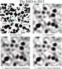 |
Fig. 17 Comparison of DSO images in the a) Ks- (13.2 mas pixel scale) and b) L′-band (27 mas pixel scale). The image section size is 1′′ × 1′′. In c) and d) a Gaussian of 98 mas FWHM and a PSF from the image have been scaled to the DSO peak brightness and subtracted at its position. An astrometric grid of red circles marks some bright stars that can be used as positional references to compare the images at different wavelengths. |
Comparing the luminosity and the magnitude of the DSO (Table 4) we obtained in the H- and Ks-band to the absolute magnitudes of OB and Be stars as presented by Wegner (2006) and stars of luminosity class I − V, we found that the DSO could preferentially be a K-dwarf (V) or an F-dwarf/subgiant (V-III) at no additional extinction intrinsic to the surrounding dust cloud or an A-dwarf/subgiant (V-III) at about 30 magn of intrinsic visual extinction (see Fig. 15). The AGB or early evolutionary phase may be included here to support the dusty envelope. These identifications point toward a slightly later type as compared to the earlier-type B0-2.5 V stars in the S-cluster (Martins et al. 2008). This would imply a stellar mass of a few solar masses. However, the combination of local extinction (including geometrical effects like shadowing and volume-filling factors of the extincting material) and scattering may alter that identification and it could be even earlier or more luminous as well. This leads us to discuss four additional scenarios: Scenario I: since the DSO is prominent in its hydrogen line emission (Gillessen et al. 2012a) with a Brγ line with of 100 km s-1 in 2008 but rather faint in the H and Ks continuum bands (see Table 4), it may very well be a dusty, faint narrow-line Wolf-Rayet (WR) star. They are known to be less luminous than most other WR or OB giants, and there are a few of these objects in the GC field (see e.g. Moultaka et al. 2005; Paumard et al. 2006). The WR stars IRS7W with mK = 13.1, IRS7SE with mK = 13.0 (Martins et al. 2007) and WR2 with mK = 12.9 (Moultaka et al. 2005) are amongst the faintest known so far in the Galactic center cluster (for faint WR stars in the Milky Way see also Shara et al. 1999, 2012; Mauerhan et al. 2011 with survey limits around mK = 15.0). Given these apparent magnitudes, the DSO would have to be an exceptionally faint WR star. The earliest WR stars with dense winds and strong free-free excesses may belong to the intrinsically faintest of the WRs (Mauerhan et al. 2011). As indicated by the increasing Brγ (Gillessen et al. 2012a), the harsh environment of the S-star cluster and the possibly repeated interaction with the SgrA* black hole may have altered the stars mass loss or shell size and hence its luminosity in the thermal infrared and the Brγ line width of an object that started out as a narrow-line WR star at larger separations from SgrA*. Scenario II: Dong et al. (2012) have carried out a multi-wavelength study of evolved massive stars in the GC. In their Fig. 12 they show a Paα equivalent line width (EW) vs. Ks-[3.6 μm] plot of these objects. From this plot it becomes obvious that for WC stars and the fainter WNL stars/OB super-giants the EW values are lower than 100 Å for Ks- [3.6 μm] > 2 mag and even drop significantly with further increasing infrared excess, reaching values of up to Ks- [3.6 μm] ~ 5. Dong et al. (2012) suggested that the free-free emission from the strong winds of the WNL stars/OB giants could potentially dominate the emission in the mid-infrared (Wright & Barlow 1975). This could explain the positive EW vs. Ks-[3.6 μm] correlation they found. These properties fit with the DSO well if we assume that Ks-[3.6 μm] ≈ Ks − L′ and that a small EW in the Paα line is correlated with a small EW of the Brγ line. The Brγ line width in 2008 indicated in Fig. 2 by Gillessen et al. (2012a) is on the order of or smaller than 100 km s-1 in 2008 and 200 km s-1 in 2011. Taking the Galactic foreground extinction into account, its position in the color−color diagram in Fig. 16 (left) comes to lie in the WNL stars/OB supergiant domain with small EW and high infrared excess, as described by Dong et al. (2012). Scenario III: Murray-Clay & Loeb (2011, 2012) have proposed that the dusty S-cluster object is a proto-planetary disk that has been brought in from a young stellar ring. However, to change the ellipticity of the previously rather circular orbit in one single event to the high ellipticity orbit on which it is now requires a similarly violent interaction as the upcoming peri-bothron passage. If the object were only a core-less dust cloud, this event would therefore lead to an early destruction of the object at the time it enters the current orbit. If the source is indeed a core-less dust cloud, the only alternative is that the ellipticity of its orbit has been changed gradually. However, this implies many peri-bothron passages, imposes a conflict with evaporation timescales, and will most likely lead to destruction as well. The only alternative is indeed that the dusty S-cluster object has been formed on an orbit rather similar to the current one, or that it has been brought in gradually from outside the S-star cluster, as proposed earlier by Murray-Clay & Loeb (2011, 2012). This hypothesis is also supported by the analysis in the color−color diagram shown in Fig. 16 (left). The authors show that there are two objects, D3 and the DSO, which are dominated by their dust emission in the L′-band, which would be the case if they were relatively young stellar objects. Scenario IV: the DSO may be similar to the bow-shock sources X3 and X7 (Muzic et al. 2010) but has not yet developed an obvious bow-shock structure. For X3 and X7 Muzic et al. (2010) discussed possible stellar counterparts, including the possibility of late-type and main-sequence sources. However, the preference is clearly on late B-type main-sequence stars (B7-8V) and low-luminosity WR stars as well. Other explanations have problems: the central star of a planetary nebulae will remain at the required brightness for less than 1000 yr before it becomes too faint, and a main-sequence star cannot be an appropriate source of a dust-rich envelope, as is apparently observed for the DSO in the L-band.
4.10. Will the DSO be disrupted?
Gillessen et al. (2012a) have reported that the Brγ emission of the DSO is spread over 200 mas. Similar sizes are also predicted in the models presented by Burkert et al. (2012) and Schartmann et al. 2012. In Fig. 17 we compare images of the DSO in the Ks- and L′-band. We also show the L′-band images after removing the DSO using a Gaussian of 98 mas FWHM (i.e., the diffraction limit in the L′-band) and a star located 0.5′′ west and 0.42′′ north of SgrA* (i.e., a PSF obtained from an image section close to SgrA*; see Fig. 1). The analysis of the images shows that >90% of the DSO emission at 3.8 μm wavelength is compact (FWHM ≤ 20 mas). Only up to 10% of the flux density contained in the compact part of the DSO can be extended on the scale size of the PSF. This indicates that the warm (~550 K) dust emission is very compact in comparison to the hotter (~104 K) hydrogen recombination line emission. Alternatively, the MIR continuum emission contains a significant compact free-free contribution (see below). In this case, however, one would expect that the recombination line emission is dominated by contributions from this free-free component and should hence be more compact than observed.
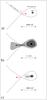 |
Fig. 18 Sketch of the relative position and motion of the Lagrange point L1 and the DSO. |
Since the Ks-band identifications of the DSO suggest that it can also be associated with a star it is only its dusty envelope that can potentially be disrupted. To investigate that possibility we have to determine the location of the Lagrange point L1 through which mass can be transferred and compare it to the size of the dust shell or disk. In Fig. 18 we show a sketch that demonstrates the location of the DSO and the motion of the Lagrange point L1 with respect to it. In panel a) in Fig. 18 we show the situation about one year before the peri-bothron passage. The L1 point is rapidly approaching the DSO through its orbital motion toward SgrA*. At peri-bothron, L1 will also be closest to the star (panel b) in Fig. 18). If the star has a mass of about 1 M⊙, the separation of L1 from it will be about 0.1 AU. For a Herbig Ae/Be stars with 2−8 M⊙ that distance will be 0.2 and 0.5 AU. For a typical S-cluster stellar mass of ~20−30 M⊙ the separation will be closer to one AU. Interferometrically determined typical inner ring sizes for young Herbig Ae/Be and T Tauri stars can be as small as 0.1−1 AU (Monnier & Millan-Gabet 2002), however, a disk or shell may be much larger than this. Based on its MIR-luminosity, Gillessen et al. (2012a) determined a source size of about 1 AU. Hence, during peri-bothron passage a significant amount of the dusty circumstellar material may pass beyond L1 and start to move into the Roche lobe associated with SgrA*.
However, this peri-bothron passage will only last for a few months, after which the DSO will move away from SgrA* at a speed of around a 1000 km s-1 within the first year. After one year the separation of the L1-point from the DSO is already about 1000 times larger than during the peri-bothron passage (panel c) in Fig. 18). This implies that any cold dusty material that passed the L1 toward the SgrA* will be overtaken again by the receding L1-point. However, the time will not be sufficient to completely disrupt the dust shell or disk of the DSO, especially if it is very compact. The material that passed he L1-point during the peri-bothron passage will not stay in the SgrA* Roche lobe and will not be immediately accreted. Only thin, hot material associated with a possible stellar wind of a hot and massive object may stay past the L1-point, but at the typical escape velocities of such volatile material of a few 100 km s-1 it would have left the star in any case.
Shcherbakov & Baganoff (2010) have discussed the feeding rate of SgrA* as a function of radius. Their modeling suggests that sources X3 and X7 (Muzic et al. 2010) are still in the regime in which most of the in-flowing mass is blown away again (see their Fig. 3). This may partly explain the bow-shock structure of X3 and X7. During its peri-bothron passage the star S2 has been well within the zone in which matter of its stellar wind could have been accreted. However, no effect on the variability of SgrA* has been reported. The DSO peri-bothron will be at a larger radius than that of S2. This implies that if the stellar wind from its central star is not stronger than that of S2, no enhanced accretion effect will result from it. If the radius-dependent accretion flow is clumpy or un-isotropic, the DSO may still develop a bow-shock like X3 and X7 and a major portion of the cold and dusty material that was detached from the DSO during its peri-bothron passage will be blown away.
5. Summary
We have shown that most of the L′-band excess sources are indeed associated with stellar objects that can be identified as H- or Ks-band sources with the same proper motions as the L′-band objects. While this is true for many of the infrared excess sources we found in the inner few arcseconds of the GC, it is also true for all objects that constitute the small association of co-moving IRS13N sources (sources β to η in the nomenclature of Eckart et al. 2004). The colors of the excess sources in the field (excepting D3 and the DSO) have brightnesses and colors that agree well with those of the narrow-line WR star candidates found in the central stellar cluster by Moultaka et al. (2005).
The IRS13N sources have visual extinctions that are higher than those of the excess sources in the field by up to 30 mag. The integral field spectroscopy shows that the IRS13N sources are located at a minimum of the CO-band-head absorption in that region. This makes it unlikely that they are dusty late-type stars older than a few Myr. Given the colors and extinctions of the IRS13N sources (β to η), they are the best candidates for being young stellar objects in the overall GC stellar cluster with ages younger than 1 Myr. They show no evidence for CO-bandhead absorption or emission and are then likely to belong to the Class I sources of spectrally featureless dusty young stars.
For the fast-moving DSO reported by Gillessen et al. (2012a) we were able to provide a Ks-band identification as well. While the H − Ks color limit point at a significant contribution of dust, there is also the possibility that the DSO is a dust-enshrouded stellar source and not a core-less cloud of gas and dust. The DSO may be a stellar source and is close to the SMBH for a few months only. This may have a significant influence on the possible disruption of its dusty envelope or disk. While the dusty material will certainly experience the gravitational pull by the SMBH SgrA*, it may be rapidly enclosed again by the DSO’s Roche lobe a few months after the peri-bothron passage (Fig. 18). While this is a possible scenario for the cold and dusty material, any fast wind possibly associated with the DSO may be accreted if it is a more massive, hot object. However, the peri-bothron passage distance to SgrA* is more than twice as large as that of S2 which did not have any reported effect on the variability of SgrA*. It may not be excluded, however, that if the DSO passes SgrA* by it may develop a bow-shock similar to sources X3 and X7 (Muzic et al. 2010). Additional monitoring of the trajectory and size evolution of the DSO as well as the variability of SgrA* are essential to achieve a complete picture of the scenario. It is probably currently not possible to reliably determine if and how much gas will be accreted. It is unclear if the object is already quite compact (as indicated by the L-band data) through the influence of earlier passages. It is unclear what the interaction with a wind from SgrA* is and how much of the material will be blown away. New and detailed simulations (beyond those given by Burkert et al. 2012; and Schartmann et al. 2012) will be needed that include the DSO identification as a stellar system and the nature of SgrA*.
If the IRS13N sources, in addition to the infrared excess sources including the DSO, are young stellar objects, this implies that the conditions of star formation at the center of the Milky Way may support a significant constant star formation rate in the overall central stellar cluster in addition to larger star formation events (in an accretion disk; Levin & Beloborodov 2003; Nayakshin & Sunyaev 2005; Nayakshin et al. 2006).
Online material
Appendix A
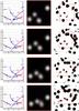 |
Fig. A.1 Ks-band identification of the DSO. We show the relative positions of the stars S23, S57, S54, S63 and the DSO over the years 2002−2012 in comparison with Ks-band Lucy-deconvolved images. The measuring uncertainties range between 13 mas and 25 mas. We show the results of the model calculation (left) with the location of the sources on their sky-projected track (dot interval 0.5 years; 1999−2006.5 in blue, 2007−2012 in red), an image of the model with the sources indicated by red circles (middle; image size is 380 mas × 380 mas), and a deconvolved Ks-band image with the modeled image section overlayed (right). For the years 2006/7 to 2012 a source can clearly be identified at the L′-band position of the DSO. The position of SgrA* is indicated by a red asterix. In the years 2002 to 2005 the DSO is confused with S63. In 2006−2008 it emerges from the confusion and shows up between the stars S23, S63, and S54 just north of S63. For 2009, 2011, 2012 the mK = 18.9 source cannot be clearly identified. This is to a large part due to the stronger crowding at the center and to the limited data quality. |
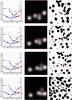 |
Fig. A.1 continued. |
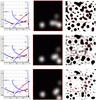 |
Fig. A.1 continued. |
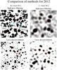 |
Fig. A.2 Retrieving the DSO in 2012 using different methods. Here we show a comparison of results from different data reduction methods and different Ks- and L′-band datasets for 2012. In both bands different methods result in a clear detection of a Ks- and L′-band counterpart of the DSO (see Ott et al. 1999, for a detailed comparison of deconvolution algorithms in the GC field). As the DSO is close to the confusion limit, the peak of the flux distribution within the diffraction limit results in small deviations in the apparent peak position. |
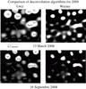 |
Fig. A.3 Retrieving the DSO in 2008 using different methods. Here we show a comparison of results from different data reduction methods and different Ks-band datasets for 2008. At both (selected as an example) epochs the different methods result in a clear detection of a Ks-band counterpart of the DSO (see also Ott et al. 1999). |
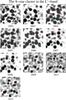 |
Fig. A.4 L′-band identification of the DSO, obtained via high-pass filtering. Here the source can always clearly be identified. For the year 2010 we have no high-quality L′-band data at hand. |
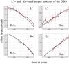 |
Fig. A.5 L′- and Ks-band coordinates of the identification of the DSO shown separately for RA and Dec values as a function of time. The 1σ deviations between the expected positions and the identifications range between ± 13 mas and ± 25 mas (i.e., a quarter of the Ks- and L′-band beam). |
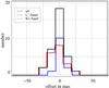 |
Fig. A.6 Histograms of the deviations from the proposed orbit (Gillessen et al. 2012) for all bands. The 1σ deviations between the expected positions and the identifications in the different bands range between ± 13 mas and ± 25 mas. |
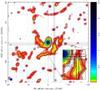 |
Fig. A.7 Mini-spiral region imaged with CARMA in the 1.3 mm CD array configuration with a synthesized circular beam size of 1.2′′ presented by Kunneriath et al. (2011). We show the map to outline the continuum emission from IRS13N. Contour levels are 0.015, 0.02, 0.03, 0.04, 0.05, 0.1, 0.6, 0.9, 1.2, 1.5, and 2.5 Jy/beam. Solid black lines and a thin cyan ellipse (in the inset) indicate in the map and the inset indicates the region in which the IRS13N sources are located. |
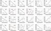 |
Fig. A.8 Ks-band proper motions of the 34 sources in and close to the IRS13E and IRS13N field. Offsets in RA and Dec in milliarcseconds are plotted against the time in years. Source labels are given as indicated in Fig. 2 and Table 3. |
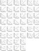 |
Fig. A.8 continued. |
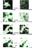 |
Fig. A.9 Comparison of the Ks- (left) and L′-band (right) identifications. L′-band excess sources in the field around SgrA* as shown in the overview map in Fig. 1 and listed in Table 4. The arrow color-coding for the observing bands and the proper motions are given between the images in the lower part of the panel. The 2004 map sizes are 0.932′′ × 0.932′′ (70 × 70 pixels) in the Ks-band and 0.945′′ × 0.945′′ (35 × 35 pixels) in the L′-band. We have indicated the sources with arrows and labels. The gray-scaling is given in bars and the contours are logarithmically spaced and given for display purposes only. The DSO is visible at the lowest contour levels in the appropriate plot in Fig. A.9. In Fig. A.9 we marked the region in which D7 is located with a dashed circle. Some contour excursions are visible, but no clear detection of a compact source is possible. For source D4/X7 see Muzic et al. (2010). |
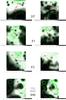 |
Fig. A.9 continued. |
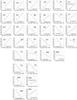 |
Fig. A.10 Proper motions of infrared excess sources in the central 2′′ close to SgrA*. Offsets in RA and Dec in milliarcseconds are plotted against the time in years. Source labels and observing bands are given as indicated in Fig. 1 and Table 4. The source positions agree to within better than about ± 25 mas, i.e., a quarter of the L′-band beam. The motions obtained at different wavebands agree within the uncertainties. For sources for which S-star identifications are given, the positions and motions agree on average to within about 30 mas and 150 km s-1. |
L′-, Ks, and H-band positions of infrared excess sources in the central 2′′ field close to SgrA*.
L′-, Ks, and H-band proper motion velocities of infrared excess sources in the central 2′′ field close to SgrA* including results from a linear fit to the DSO data.
Based on observations collected at the European Southern Observatory, Chile.
Acknowledgments
We thank the anonymous referee for the useful comments and suggestions that helped to improve the paper. This work was supported in part by the Deutsche Forschungsgemeinschaft (DFG) via the Cologne Bonn Graduate School (BCGS), the Max Planck Society through the International Max Planck Research School (IMPRS) for Astronomy and Astrophysics, as well as special funds through the University of Cologne. B. Shahzamanian, N. Sabha and M. Valencia-S., are members of the IMPRS. N. Sabha is member of the Bonn Cologne Graduate School for Physics and Astronomy. Part of this work was supported by the German Deutsche Forschungsgemeinschaft, DFG, via grant SFB 956, and by fruitful discussions with members of the European Union funded COST Action MP0905: Black Holes in a violent Universe and PECS project No. 98040. This work was co-funded under the Marie Curie Actions of the European Commission (FP7-COFUND). Macarena García-Marín is supported by the German federal department for education and research (BMBF) under the project number 50OS1101. NSO/Kitt Peak FTS data used here were produced by NSF/NOAO. We are grateful to all members of the NAOS/CONICA and the ESO PARANAL team.
References
- Baganoff, F. K., Bautz, M. W., Brandt, W. N., et al. 2001, Nature, 413, 45 [NASA ADS] [CrossRef] [PubMed] [Google Scholar]
- Baganoff, F. K., Maeda, Y., Morris, M., Bautz, M. W., et al. 2003, ApJ, 591, 891 [NASA ADS] [CrossRef] [Google Scholar]
- Bartko, H., Martins, F., Trippe, S., Fritz, T. K., Genzel, R., et al. 2010, ApJ, 708, 834 [NASA ADS] [CrossRef] [Google Scholar]
- Berukoff, S. J., & Hansen, B. M. S. 2006, ApJ, 650, 901 [NASA ADS] [CrossRef] [Google Scholar]
- Brandner, W., Rousset, G., Lenzen, R., et al. 2002, Msngr, 107, 1 [Google Scholar]
- Bremer, M., Witzel, G., Eckart, A., et al. 2011, A&A, 532, A26 [NASA ADS] [CrossRef] [EDP Sciences] [Google Scholar]
- Buchholz, R. M., Schödel, R., & Eckart, A. 2009, A&A, 499, 483 [NASA ADS] [CrossRef] [EDP Sciences] [Google Scholar]
- Burkert, A., Schartmann, M., Alig, C., et al. 2012, ApJ, 750, 58 [NASA ADS] [CrossRef] [Google Scholar]
- Calvet, N., Hartmann, L., & Strom, S. E. 1997, ApJ, 481, 912 [NASA ADS] [CrossRef] [Google Scholar]
- Casali, M. M., & Eiroa, C. 1996, A&A, 306, 427 [NASA ADS] [Google Scholar]
- Coker, R. F., Pittard, J. M., & Kastner, J. H. 2002, A&A, 383, 568 [NASA ADS] [CrossRef] [EDP Sciences] [Google Scholar]
- Clenet, Y., Roun, D., Gratadour, D., et al. 2005, A&A, 439, 9 [Google Scholar]
- Crowther, P. A. 2001, in The influence of binaries on stellar population studies (Dordrecht: Kluwer Academic Publishers), Astrophys. Space science Lib. (ASSL), 264, 215 [Google Scholar]
- Dong, H., Wang, Q. D., & Morris, M. R. 2012, MNRAS, 425, 884 [NASA ADS] [CrossRef] [Google Scholar]
- Diolaiti, E., Bendinelli, O., Bonaccini, D., et al. 2000, SPIE, 4007, 879 [NASA ADS] [Google Scholar]
- Drake, S. A., & Linsky, J. L. 1989, AJ, 98, 1831 [NASA ADS] [CrossRef] [Google Scholar]
- Eckart, A., & Genzel, R. 1996, Nature, 383, 415 [NASA ADS] [CrossRef] [Google Scholar]
- Eckart, A., Ott, T., & Genzel, R. 1999, A&A, 352, L22 [NASA ADS] [Google Scholar]
- Eckart, A., Genzel, R., Ott, T., & Schödel, R. 2002, MNRAS, 331, 917 [NASA ADS] [CrossRef] [Google Scholar]
- Eckart, A., Moultaka, J., Viehmann, T., Straubmeier, C., & Mouawad, N. 2004, ApJ, 602, 760 [CrossRef] [Google Scholar]
- Eckart, A., Baganoff, F. K., Schödel, R., et al. 2006, A&A, 450, 535 [NASA ADS] [CrossRef] [EDP Sciences] [Google Scholar]
- Eckart, A., Sabha, N., Witzel, G., et al. 2012, Conf. Proc. SPIE, in press [arXiv:1208.1129E] [Google Scholar]
- Eisenhauer, F., Abuter, R., Bickert, K., et al. 2003, SPIE, 4841, 1548 [NASA ADS] [Google Scholar]
- Fritz, T. K., Gillessen, S., Dodds-Eden, K., et al. 2010, ApJ, 721, 395 [NASA ADS] [CrossRef] [Google Scholar]
- Fuente, A., Martin-Pintado, J., Bachiller, R., Rodriguez-Franco, A., & Palla, F. 2002, A&A, 387, 977 [NASA ADS] [CrossRef] [EDP Sciences] [Google Scholar]
- Ghez, A., Morris, M., Becklin, E. E., Tanner, A., & Kremenek, T. 2000, Nature, 407, 349 [NASA ADS] [CrossRef] [PubMed] [Google Scholar]
- Glass, I. S., & Moorwood, A. F. M. 1985, MNRAS, 214, 429 [NASA ADS] [CrossRef] [Google Scholar]
- Green, T. P., & Meyer, M. R. 1995, ApJ, 450, 233 [NASA ADS] [CrossRef] [Google Scholar]
- Genzel, R., Schödel, R., Ott, T., et al. 2003, ApJ, 594, 812 [NASA ADS] [CrossRef] [PubMed] [Google Scholar]
- Gerhard, O. 2001, ApJ, 546, L39 [NASA ADS] [CrossRef] [Google Scholar]
- Ghez, A. M., Salim, S., Hornstein, S. D., et al. 2005, ApJ, 620, 744 [NASA ADS] [CrossRef] [Google Scholar]
- Gillessen, S., Eisenhauer, F., Trippe, S. et al. 2009, ApJ, 692, 1075 [NASA ADS] [CrossRef] [Google Scholar]
- Gillessen, S., Genzel, R., Fritz, T. K., et al. 2012a, Nature, 481, 51 [NASA ADS] [CrossRef] [Google Scholar]
- Gillessen, S., Genzel, R., Fritz, T. K., et al. 2012b, ApJ, submitted [arXiv:1209.2272] [Google Scholar]
- Hansen, B. M. S., & Milosavljevic, M. 2003, ApJ, 593, L77 [NASA ADS] [CrossRef] [Google Scholar]
- Hillenbrand, L. A., Strom, S. E., Vrba, F. J., & Keene, J. 1992, ApJ, 397, 613 [NASA ADS] [CrossRef] [Google Scholar]
- Hoffmeister, V. H., Chini, R., Scheyda, C. D., et al. 2006, A&A, 457, L29 [NASA ADS] [CrossRef] [EDP Sciences] [Google Scholar]
- Ishii, M., Nagata, T., Sato, S., et al. 1998, AJ, 116, 868 [NASA ADS] [CrossRef] [Google Scholar]
- Kim, S. S., Figer, D. F., & Morris, M. 2004, ApJ, 607, L123 [NASA ADS] [CrossRef] [Google Scholar]
- Kudritzki, R. P., Puls, J., Lennon, et al. 1999, A&A, 350, 970 [NASA ADS] [Google Scholar]
- Kunneriath, D., Eckart, A., Vogel, S. N., et al. 2012a, A&A, 538, A127 [CrossRef] [EDP Sciences] [Google Scholar]
- Kunneriath, D., Eckart, A., Vogel, S. N., et al. 2012b, PhCS, 372, 2063 [NASA ADS] [Google Scholar]
- Lang, C. C., Johnson, K. E., Goss, W. M., & Rodrguez, L. F. 2005, AJ, 130, 2185 [Google Scholar]
- Lenzen, R., Hofmann, R., Bizenberger, P., & Tusche, A. 1998, SPIE, 3354, 606 [Google Scholar]
- Levin, Y., & Beloborodov, A. M. 2003, ApJ, 590, L33 [NASA ADS] [CrossRef] [Google Scholar]
- Lu, J. R., Ghez, A. M., Hornstein, S. D., Morris, M., & Becklin, E. E. 2005, ApJ, 625, L51 [NASA ADS] [CrossRef] [Google Scholar]
- Lu, J. R., Ghez, A. M., Hornstein, S. D., et al. 2009, ApJ, 690, 1463 [NASA ADS] [CrossRef] [Google Scholar]
- Luhman, K. L., & Rieke, G. H. 1999, ApJ, 525, 440 [NASA ADS] [CrossRef] [Google Scholar]
- Lutz, D., Feuchtgruber, H., Genzel, R., et al. 1996, A&A, 315, L269 [NASA ADS] [Google Scholar]
- Maillard, J. P., Paumard, T., Stolovy, S. R., & Rigaut, F. 2004, A&A, 423, 155 [NASA ADS] [CrossRef] [EDP Sciences] [Google Scholar]
- Martins, F., Genzel, R., Hillier, D. J., et al. 2007, A&A, 468, 233 [NASA ADS] [CrossRef] [EDP Sciences] [Google Scholar]
- Martins, F., Gillessen, S., Eisenhauer, F., et al. 2008, ApJ, 672, L119 [NASA ADS] [CrossRef] [Google Scholar]
- Mauerhan, J. C., Van Dyk, S. D., & Morris, P. W. 2011, AJ, 142, 40 [NASA ADS] [CrossRef] [Google Scholar]
- McMillan, S. L. W., & Portegies Zwart, S. F. 2003, ApJ, 596, 314 [NASA ADS] [CrossRef] [Google Scholar]
- Milosavljevic, M, & Loeb, A. 2004, ApJ, 604, L45 [NASA ADS] [CrossRef] [Google Scholar]
- Molinari, S., Pezzuto, S., Cesaroni, R., et al. 2008, A&A, 481, 345 [NASA ADS] [CrossRef] [EDP Sciences] [Google Scholar]
- Monnier, J. D., & Millan-Gabet, R., 2002, ApJ, 579, 694 [NASA ADS] [CrossRef] [Google Scholar]
- Montes, G., Perez-Torres, M. A., Alberdi, A., & Gonzalez, R. F. 2009, ApJ, 705, 899 [NASA ADS] [CrossRef] [Google Scholar]
- Moultaka, J., Eckart, A., Schödel, R., Viehmann, T., & Najarro, F. 2005, A&A, 443, 163 [NASA ADS] [CrossRef] [EDP Sciences] [Google Scholar]
- Murray-Clay, R. A., & Loeb, A. 2011 [arXiv:1112.4822M] [Google Scholar]
- Murray-Clay, R. A., & Loeb, A. 2012, NatCo, 3, 1049 [Google Scholar]
- Muzic, K., Eckart, A., Schödel, R., Meyer, L., & Zensus, A. 2007, A&A, 469, 993 [NASA ADS] [CrossRef] [EDP Sciences] [Google Scholar]
- Muzic, K., Schödel, R., Eckart, A., Meyer, L., & Zensus, A. 2008, A&A, 482, 173 [NASA ADS] [CrossRef] [EDP Sciences] [Google Scholar]
- Muzic, K., Eckart, A., Schödel, R., et al. 2010, A&A, 521, A13 [NASA ADS] [CrossRef] [EDP Sciences] [Google Scholar]
- Nayakshin, S., & Sunyaev, R. 2005, MNRAS, 364, L23 [NASA ADS] [CrossRef] [Google Scholar]
- Nayakshin, S., Dehnen, W., Cuadra, J., & Genzel, R. 2006, MNRAS, 366, 1410 [NASA ADS] [CrossRef] [Google Scholar]
- Nayakshin, S., Cuadra, J., & Springel, V. 2007, MNRAS, 379, 21 [NASA ADS] [CrossRef] [Google Scholar]
- Ott, T., Eckart, A., & Genzel, R. 1999, ApJ, 523, 248 [NASA ADS] [CrossRef] [Google Scholar]
- Paumard, T., Maillard, J.-P., & Morris, M. 2004, A&A, 426, 81 [NASA ADS] [CrossRef] [EDP Sciences] [Google Scholar]
- Paumard, T., Genzel, R., Martins, F., et al. 2006, ApJ, 643, 1011 [NASA ADS] [CrossRef] [Google Scholar]
- Perger, M., Moultaka, J., Eckart, A., et al. 2008, A&A, 478, 127 [NASA ADS] [CrossRef] [EDP Sciences] [Google Scholar]
- Portegies Zwart, S. F., Baumgardt, H., McMillan, S. L. W., et al. 2006, ApJ, 641, 319 [NASA ADS] [CrossRef] [Google Scholar]
- Prato, L., Lockhart, K. E., Johns-Krull, C. M., & Rayner, J. T. 2009, AJ, 137, 3931 [NASA ADS] [CrossRef] [Google Scholar]
- Rousset, G., Lacombe, F., Puget, P., et al. 1998, SPIE, 3353, 508 [Google Scholar]
- Sabha, N., Witzel, G., Eckart, A., et al. 2010, A&A, 512, A2 [NASA ADS] [CrossRef] [EDP Sciences] [Google Scholar]
- Sabha, N., Eckart, A., Merritt, D., et al. 2012, A&A, 545, A70 [NASA ADS] [CrossRef] [EDP Sciences] [Google Scholar]
- Scally, A., & Clarke, C. 2001, MNRAS, 325, 449 [Google Scholar]
- Schartmann, M., Burkert, A., Alig, C., et al. 2012, ApJ, 755, 155 [NASA ADS] [CrossRef] [Google Scholar]
- Schödel, R., Eckart, A., Iserlohe, C., Genzel, R., & Ott, T. 2005, ApJ, 625, L111 [NASA ADS] [CrossRef] [Google Scholar]
- Schödel, R., Merritt, D., & Eckart, A. 2009, A&A, 502, 91 [NASA ADS] [CrossRef] [EDP Sciences] [Google Scholar]
- Schödel, R., Najarro, F., Muzic, K., & Eckart, A. 2010, A&A, 511, A18 [NASA ADS] [CrossRef] [EDP Sciences] [Google Scholar]
- Shcherbakov, R. V., & Baganoff, F. K. 2010, ApJ, 716, 504 [NASA ADS] [CrossRef] [Google Scholar]
- Shara, M. M., Moffat, A. F. J., Smith, L. F., et al. 1999, AJ, 118, 390 [NASA ADS] [CrossRef] [Google Scholar]
- Shara, M. M., Faherty, J. K., Zurek, D., et al. 2012, AJ, 143, 149 [NASA ADS] [CrossRef] [Google Scholar]
- Stolte, A., Ghez, A., Morris, M., et al. 2009, Ap&SS, 324, 137 [NASA ADS] [CrossRef] [Google Scholar]
- Stolte, A., Morris, M. R., Ghez, A. M., et al. 2010, ApJ, 718, 810 [NASA ADS] [CrossRef] [Google Scholar]
- Tanner, A., Ghez, A. M., Morris, M. R., & Christou, J. C. 2005, ApJ, 624, 742 [NASA ADS] [CrossRef] [Google Scholar]
- van Kempen, T. A., van Dishoeck, E. F., Salter, D. M., et al. 2009, A&A, 498, 167 [NASA ADS] [CrossRef] [EDP Sciences] [Google Scholar]
- Viehmann, T., Eckart, A., Schödel, R., et al. 2005, A&A, 433, 117 [NASA ADS] [CrossRef] [EDP Sciences] [Google Scholar]
- Viehmann, T., Eckart, A., Schödel, R., Pott, J.-U., & Moultaka, J. 2006, ApJ, 642, 861 [NASA ADS] [CrossRef] [Google Scholar]
- Wegner, W. 2006, MNRAS, 371, 185 [NASA ADS] [CrossRef] [Google Scholar]
- Witzel, G., Eckart, A., Bremer, M., et al. 2012, ApJS, 203, 18 [NASA ADS] [CrossRef] [Google Scholar]
- Wright, A. E., & Barlow, M. J. 1975, MNRAS, 170, 41 [NASA ADS] [CrossRef] [Google Scholar]
- Zhao, J.-H., & Goss, W. M. 1998, ApJ, 499, L163 [NASA ADS] [CrossRef] [Google Scholar]
- Zhao, J.-H., Morris, M. R., Goss, W. M., & An, T. 2009, ApJ, 699, 186 [NASA ADS] [CrossRef] [Google Scholar]
All Tables
Relative and absolute coordinates of the lower left (southeastern) corner of the image sections shown in the corresponding figure.
Ks-band positions in arcseconds relative to SgrA* and proper motions in km s-1 of IRS13E and IRS13N sources at epoch 2005.83.
Names, positional offsets from SgrA* in arcseconds, proper motions in km s-1 of compact infrared excess sources in the central 2′′ field close to SgrA*.
Ks-, and L′-band positions of the DSO and the star S2 relative to the SgrA* position.
L′-, Ks, and H-band positions of infrared excess sources in the central 2′′ field close to SgrA*.
L′-, Ks, and H-band proper motion velocities of infrared excess sources in the central 2′′ field close to SgrA* including results from a linear fit to the DSO data.
All Figures
|
Fig. 1 Proper motion vectors of dusty objects in the central stellar cluster of the Milky Way (see Table 4). We show the May 10, 2003, adaptive optics L′-band image of the central 4′′ × 4′′. The arrows indicate the uncertainties in amount (red or yellow portion of the otherwise green arrow) and angle of the measured proper motion derived from data between 2002 and 2008 in the H, Ks, and L′-bands (see Table 1). |
| In the text | |
|
Fig. 2 High-pass-filtered image of the IRS13E/IRS13N field in the Ks-band. The labels correspond to those in Table 3. Source 1 to 6 are sources E1 to E6 in IRS13E. The angular resolution is close to the diffraction limit of 60 mas. |
| In the text | |
|
Fig. 3 Wavelength-integrated 2 μm SINFONI data cube. Yellow circles mark the regions in which the spectra were obtained. The angular resolution is about 0.11 arcsec. |
| In the text | |
|
Fig. 4 Ks-band identification of individual IRS13E and IRS13N sources at two different epochs and visualizations of the positions of the IRS13N sources α, β, δ, ϵ, η, and κ at two different epochs. The source labels in the high-pass filtered images correspond to those in Table 3. |
| In the text | |
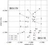 |
Fig. 5 Proper motion of IRS13E and IRS13N. For source labels see Figs. 4 and 6. |
| In the text | |
|
Fig. 6 Visualization of the Ks-band identifications of the IRS13N sources γ, δ, ϵ, and ζ at four different epochs in high-pass filtered images. The source labels correspond to those in Table 3. |
| In the text | |
|
Fig. 7 Comparison of Ks- and L′-band proper motions in right ascension and declination for the GC IRS13E and the IRS13N cluster (indicated by circles in dashed lines). The direction of the motion, i.e., S to N, or E to W, is labeled. The source labels correspond to those in Table 3. The Ks-band motions derived here are labeled with open dots. For IRS13 and for IRS13N the filled dots indicate the proper motions published by Fritz et al. (2010) and Muzic et al. (2008). The open circles depict the Ks-band proper motions described here. |
| In the text | |
|
Fig. 8 2 μm-band image (left; IB 2.15 μm) and L′-band image (right; 3.8 μm) with the Brγ emission (top) and CO absorption (bottom) line maps in contours overplotted. |
| In the text | |
|
Fig. 9 2 μm-band image (left; IB 2.15 micron) and L′-band image (right; 3.8 μm) with [FeIII]-emission line maps in contours overplotted. |
| In the text | |
|
Fig. 10 13 mm VLA radio image from Zhao et al. (2009) with our Brγ- and [FeIII]-emission line maps in contours overplotted. |
| In the text | |
|
Fig. 11 Integrated Ks-band spectrum of IRS13N (top panel), spectrum of the nearby region Diffuse-1 west of IRS13N (middle panel) and Diffuse-2 east of IRS13N (bottom). The three spectra were normalized to the peak value of the Brγ line in the IRS13N spectrum. The spectra are continuum subtracted. |
| In the text | |
|
Fig. 12 Integrated Ks-band spectrum of the [FeIII]-emission line source at the position of source K21 (Zhao et al. 2009) north of IRS13 N. This spectrum is continuum subtracted normalized to the peak of the Brγ line. |
| In the text | |
|
Fig. 13 Distinguishing the DSO against stars S57, S23, S54, and S63 in 2008 in L′- and Ks-band. Only an upper limit can be given in the H-band. |
| In the text | |
|
Fig. 14 Positions of the DSO relative to S2 and SgrA* plotted in comparison to the orbital tracks provided by Gillessen et al. (2012a) (red for the DSO, blue for S2, SgrA* is at the position of the black dot at the origin). The results for the Ks- and L′-band are shown in panels a) and b) (see data in Table 5). Thin lines indicate the approximate expected positions of the DSO on its orbit from 2002.0 to 2012.0 (based on our L′-band reductions and Gillessen et al. 2012a). The epochs are color-coded and the measurement uncertainty is shown as a black cross (see A.6 in the appendix). |
| In the text | |
|
Fig. 15 Decomposition of the DSO spectrum including our Ks-band detection and H-band limit. Here we demonstrate that a mixture of dust and stellar contribution is possible. The points correspond to the L- and Ks-band magnitudes, and H-band upper limit from this work, and the M-band measurement and K-band upper limit of Gillessen et al. (2012a,b). Red and blue dashed curves also show their 550 K and 650 K warm dust fits. In solid blue, red, and magenta lines the emission from three different possible stellar types of the DSO core are plotted. Any of these stars embedded in 450 K dust (solid brown line) can produce the black line that fits all the NIR DSO photometric measurements. |
| In the text | |
|
Fig. 16 Left: colors of dusty objects in the central parsec of the Milky Way compared to the colors of young stellar objects as given by Hoffmeister et al. (2006). The labels COAS and COES indicate that the sources show CO absorption or emission in their spectra. Right: colors of dusty objects in the central parsec of the Milky Way compared to colors of pure dust (temperatures given in red numbers) and mixtures of a stellar and a dust contribution (fractional numbers given in black; see also Glass & Moorwood 1985). Here we demonstrate that a mixture of dust and stellar contribution is possible. Because the H − Ks color of DSO is an upper limit, its NIR emission can be explained as pure dust at 550 K reddened by ~27 mag, or as a star embedded in warm dust, e.g., if its color were detected to be H − KS ~ 3.5 mag (dashed circle), after dereddening by 27 mag, its emission would be consistent with 20% stellar and 80% dust contributions. |
| In the text | |
|
Fig. 17 Comparison of DSO images in the a) Ks- (13.2 mas pixel scale) and b) L′-band (27 mas pixel scale). The image section size is 1′′ × 1′′. In c) and d) a Gaussian of 98 mas FWHM and a PSF from the image have been scaled to the DSO peak brightness and subtracted at its position. An astrometric grid of red circles marks some bright stars that can be used as positional references to compare the images at different wavelengths. |
| In the text | |
|
Fig. 18 Sketch of the relative position and motion of the Lagrange point L1 and the DSO. |
| In the text | |
|
Fig. A.1 Ks-band identification of the DSO. We show the relative positions of the stars S23, S57, S54, S63 and the DSO over the years 2002−2012 in comparison with Ks-band Lucy-deconvolved images. The measuring uncertainties range between 13 mas and 25 mas. We show the results of the model calculation (left) with the location of the sources on their sky-projected track (dot interval 0.5 years; 1999−2006.5 in blue, 2007−2012 in red), an image of the model with the sources indicated by red circles (middle; image size is 380 mas × 380 mas), and a deconvolved Ks-band image with the modeled image section overlayed (right). For the years 2006/7 to 2012 a source can clearly be identified at the L′-band position of the DSO. The position of SgrA* is indicated by a red asterix. In the years 2002 to 2005 the DSO is confused with S63. In 2006−2008 it emerges from the confusion and shows up between the stars S23, S63, and S54 just north of S63. For 2009, 2011, 2012 the mK = 18.9 source cannot be clearly identified. This is to a large part due to the stronger crowding at the center and to the limited data quality. |
| In the text | |
|
Fig. A.1 continued. |
| In the text | |
|
Fig. A.1 continued. |
| In the text | |
|
Fig. A.2 Retrieving the DSO in 2012 using different methods. Here we show a comparison of results from different data reduction methods and different Ks- and L′-band datasets for 2012. In both bands different methods result in a clear detection of a Ks- and L′-band counterpart of the DSO (see Ott et al. 1999, for a detailed comparison of deconvolution algorithms in the GC field). As the DSO is close to the confusion limit, the peak of the flux distribution within the diffraction limit results in small deviations in the apparent peak position. |
| In the text | |
|
Fig. A.3 Retrieving the DSO in 2008 using different methods. Here we show a comparison of results from different data reduction methods and different Ks-band datasets for 2008. At both (selected as an example) epochs the different methods result in a clear detection of a Ks-band counterpart of the DSO (see also Ott et al. 1999). |
| In the text | |
|
Fig. A.4 L′-band identification of the DSO, obtained via high-pass filtering. Here the source can always clearly be identified. For the year 2010 we have no high-quality L′-band data at hand. |
| In the text | |
|
Fig. A.5 L′- and Ks-band coordinates of the identification of the DSO shown separately for RA and Dec values as a function of time. The 1σ deviations between the expected positions and the identifications range between ± 13 mas and ± 25 mas (i.e., a quarter of the Ks- and L′-band beam). |
| In the text | |
|
Fig. A.6 Histograms of the deviations from the proposed orbit (Gillessen et al. 2012) for all bands. The 1σ deviations between the expected positions and the identifications in the different bands range between ± 13 mas and ± 25 mas. |
| In the text | |
|
Fig. A.7 Mini-spiral region imaged with CARMA in the 1.3 mm CD array configuration with a synthesized circular beam size of 1.2′′ presented by Kunneriath et al. (2011). We show the map to outline the continuum emission from IRS13N. Contour levels are 0.015, 0.02, 0.03, 0.04, 0.05, 0.1, 0.6, 0.9, 1.2, 1.5, and 2.5 Jy/beam. Solid black lines and a thin cyan ellipse (in the inset) indicate in the map and the inset indicates the region in which the IRS13N sources are located. |
| In the text | |
|
Fig. A.8 Ks-band proper motions of the 34 sources in and close to the IRS13E and IRS13N field. Offsets in RA and Dec in milliarcseconds are plotted against the time in years. Source labels are given as indicated in Fig. 2 and Table 3. |
| In the text | |
|
Fig. A.8 continued. |
| In the text | |
|
Fig. A.9 Comparison of the Ks- (left) and L′-band (right) identifications. L′-band excess sources in the field around SgrA* as shown in the overview map in Fig. 1 and listed in Table 4. The arrow color-coding for the observing bands and the proper motions are given between the images in the lower part of the panel. The 2004 map sizes are 0.932′′ × 0.932′′ (70 × 70 pixels) in the Ks-band and 0.945′′ × 0.945′′ (35 × 35 pixels) in the L′-band. We have indicated the sources with arrows and labels. The gray-scaling is given in bars and the contours are logarithmically spaced and given for display purposes only. The DSO is visible at the lowest contour levels in the appropriate plot in Fig. A.9. In Fig. A.9 we marked the region in which D7 is located with a dashed circle. Some contour excursions are visible, but no clear detection of a compact source is possible. For source D4/X7 see Muzic et al. (2010). |
| In the text | |
|
Fig. A.9 continued. |
| In the text | |
|
Fig. A.10 Proper motions of infrared excess sources in the central 2′′ close to SgrA*. Offsets in RA and Dec in milliarcseconds are plotted against the time in years. Source labels and observing bands are given as indicated in Fig. 1 and Table 4. The source positions agree to within better than about ± 25 mas, i.e., a quarter of the L′-band beam. The motions obtained at different wavebands agree within the uncertainties. For sources for which S-star identifications are given, the positions and motions agree on average to within about 30 mas and 150 km s-1. |
| In the text | |
Current usage metrics show cumulative count of Article Views (full-text article views including HTML views, PDF and ePub downloads, according to the available data) and Abstracts Views on Vision4Press platform.
Data correspond to usage on the plateform after 2015. The current usage metrics is available 48-96 hours after online publication and is updated daily on week days.
Initial download of the metrics may take a while.