| Issue |
A&A
Volume 551, March 2013
|
|
|---|---|---|
| Article Number | A18 | |
| Number of page(s) | 31 | |
| Section | Galactic structure, stellar clusters and populations | |
| DOI | https://doi.org/10.1051/0004-6361/201219994 | |
| Published online | 12 February 2013 | |
Online material
Appendix A
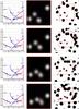 |
Fig. A.1
Ks-band identification of the DSO. We show the relative positions of the stars S23, S57, S54, S63 and the DSO over the years 2002−2012 in comparison with Ks-band Lucy-deconvolved images. The measuring uncertainties range between 13 mas and 25 mas. We show the results of the model calculation (left) with the location of the sources on their sky-projected track (dot interval 0.5 years; 1999−2006.5 in blue, 2007−2012 in red), an image of the model with the sources indicated by red circles (middle; image size is 380 mas × 380 mas), and a deconvolved Ks-band image with the modeled image section overlayed (right). For the years 2006/7 to 2012 a source can clearly be identified at the L′-band position of the DSO. The position of SgrA* is indicated by a red asterix. In the years 2002 to 2005 the DSO is confused with S63. In 2006−2008 it emerges from the confusion and shows up between the stars S23, S63, and S54 just north of S63. For 2009, 2011, 2012 the mK = 18.9 source cannot be clearly identified. This is to a large part due to the stronger crowding at the center and to the limited data quality. |
| Open with DEXTER | |
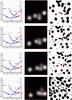 |
Fig. A.1
continued. |
| Open with DEXTER | |
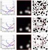 |
Fig. A.1
continued. |
| Open with DEXTER | |
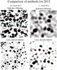 |
Fig. A.2
Retrieving the DSO in 2012 using different methods. Here we show a comparison of results from different data reduction methods and different Ks- and L′-band datasets for 2012. In both bands different methods result in a clear detection of a Ks- and L′-band counterpart of the DSO (see Ott et al. 1999, for a detailed comparison of deconvolution algorithms in the GC field). As the DSO is close to the confusion limit, the peak of the flux distribution within the diffraction limit results in small deviations in the apparent peak position. |
| Open with DEXTER | |
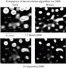 |
Fig. A.3
Retrieving the DSO in 2008 using different methods. Here we show a comparison of results from different data reduction methods and different Ks-band datasets for 2008. At both (selected as an example) epochs the different methods result in a clear detection of a Ks-band counterpart of the DSO (see also Ott et al. 1999). |
| Open with DEXTER | |
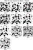 |
Fig. A.4
L′-band identification of the DSO, obtained via high-pass filtering. Here the source can always clearly be identified. For the year 2010 we have no high-quality L′-band data at hand. |
| Open with DEXTER | |
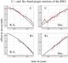 |
Fig. A.5
L′- and Ks-band coordinates of the identification of the DSO shown separately for RA and Dec values as a function of time. The 1σ deviations between the expected positions and the identifications range between ± 13 mas and ± 25 mas (i.e., a quarter of the Ks- and L′-band beam). |
| Open with DEXTER | |
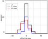 |
Fig. A.6
Histograms of the deviations from the proposed orbit (Gillessen et al. 2012) for all bands. The 1σ deviations between the expected positions and the identifications in the different bands range between ± 13 mas and ± 25 mas. |
| Open with DEXTER | |
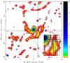 |
Fig. A.7
Mini-spiral region imaged with CARMA in the 1.3 mm CD array configuration with a synthesized circular beam size of 1.2′′ presented by Kunneriath et al. (2011). We show the map to outline the continuum emission from IRS13N. Contour levels are 0.015, 0.02, 0.03, 0.04, 0.05, 0.1, 0.6, 0.9, 1.2, 1.5, and 2.5 Jy/beam. Solid black lines and a thin cyan ellipse (in the inset) indicate in the map and the inset indicates the region in which the IRS13N sources are located. |
| Open with DEXTER | |
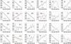 |
Fig. A.8
Ks-band proper motions of the 34 sources in and close to the IRS13E and IRS13N field. Offsets in RA and Dec in milliarcseconds are plotted against the time in years. Source labels are given as indicated in Fig. 2 and Table 3. |
| Open with DEXTER | |
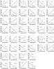 |
Fig. A.8
continued. |
| Open with DEXTER | |
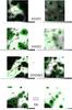 |
Fig. A.9
Comparison of the Ks- (left) and L′-band (right) identifications. L′-band excess sources in the field around SgrA* as shown in the overview map in Fig. 1 and listed in Table 4. The arrow color-coding for the observing bands and the proper motions are given between the images in the lower part of the panel. The 2004 map sizes are 0.932′′ × 0.932′′ (70 × 70 pixels) in the Ks-band and 0.945′′ × 0.945′′ (35 × 35 pixels) in the L′-band. We have indicated the sources with arrows and labels. The gray-scaling is given in bars and the contours are logarithmically spaced and given for display purposes only. The DSO is visible at the lowest contour levels in the appropriate plot in Fig. A.9. In Fig. A.9 we marked the region in which D7 is located with a dashed circle. Some contour excursions are visible, but no clear detection of a compact source is possible. For source D4/X7 see Muzic et al. (2010). |
| Open with DEXTER | |
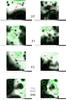 |
Fig. A.9
continued. |
| Open with DEXTER | |
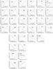 |
Fig. A.10
Proper motions of infrared excess sources in the central 2′′ close to SgrA*. Offsets in RA and Dec in milliarcseconds are plotted against the time in years. Source labels and observing bands are given as indicated in Fig. 1 and Table 4. The source positions agree to within better than about ± 25 mas, i.e., a quarter of the L′-band beam. The motions obtained at different wavebands agree within the uncertainties. For sources for which S-star identifications are given, the positions and motions agree on average to within about 30 mas and 150 km s-1. |
| Open with DEXTER | |
L′-, Ks, and H-band positions of infrared excess sources in the central 2′′ field close to SgrA*.
L′-, Ks, and H-band proper motion velocities of infrared excess sources in the central 2′′ field close to SgrA* including results from a linear fit to the DSO data.
© ESO, 2013
Current usage metrics show cumulative count of Article Views (full-text article views including HTML views, PDF and ePub downloads, according to the available data) and Abstracts Views on Vision4Press platform.
Data correspond to usage on the plateform after 2015. The current usage metrics is available 48-96 hours after online publication and is updated daily on week days.
Initial download of the metrics may take a while.