| Issue |
A&A
Volume 549, January 2013
|
|
|---|---|---|
| Article Number | A17 | |
| Number of page(s) | 20 | |
| Section | Extragalactic astronomy | |
| DOI | https://doi.org/10.1051/0004-6361/201219436 | |
| Published online | 06 December 2012 | |
Dense gas in M 33 (HerM33es)⋆,⋆⋆,⋆⋆⋆
1 Instituto Radioastronomía Milimétrica, Av. Divina Pastora 7, Nucleo Central, 18012 Granada, Spain
e-mail: buchbend@iram.es
2 Sterrewacht Leiden, Leiden University, PO Box 9513, 2300 RA Leiden, The Netherlands
3 Observatorio Astronómico Nacional (OAN)-Observatorio de Madrid, Alfonso XII 3, 28014 Madrid, Spain
4 Leiden Observatory, Leiden University, PO Box 9513, 2300 RA Leiden, The Netherlands
5 Laboratoire d’Astrophysique de Bordeaux, Université de Bordeaux, OASU, CNRS/INSU, 33271 Floirac, France
6 University of British Columbia Okanagan, 3333 University Way, Kelowna BC V1V 1V7, Canada
7 Department of Astronomy & Astrophysics, Tata Institute of Fundamental Research, Homi Bhabha Road, Mumbai 400005, India
8 Department of Earth and Space Sciences, Chalmers University of Technology, Onsala Observatory, 439 94 Onsala, Sweden
9 Laboratoire d’Astrophysique de Marseille – LAM, Université Aix-Marseille, CNRS, UMR 7326, 38 rue F. Joliot-Curie, 13388 Marseille Cedex 13, France
10 IRAM, 300 rue de la Piscine, 38406 Saint Martin d’Hères, France
11 Max-Planck Institut für Radioastronomie (MPIfR), Auf dem Hügel 69, 53121 Bonn, Germany
12 Departamento de Astrofísica, Centro de Astrobiología, CSIC-INTA, Ctra. de Torrejón a Ajalvir km 4, 28850 Madrid, Spain
13 Dept. Física Teórica y del Cosmos, Universidad de Granada, Spain
14 SRON Netherlands Institute for Space Research, Landleven 12, 9747 AD Groningen, The Netherlands
15 Astron. Dept., King Abdulaziz University, PO Box 80203, Jeddah, Saudi Arabia
Received: 18 April 2012
Accepted: 20 September 2012
Aims. We aim to better understand the emission of molecular tracers of the diffuse and dense gas in giant molecular clouds and the influence that metallicity, optical extinction, density, far-UV field, and star formation rate have on these tracers.
Methods. Using the IRAM 30 m telescope, we detected HCN, HCO+, 12CO, and 13CO in six GMCs along the major axis of M 33 at a resolution of ~114 pc and out to a radial distance of 3.4 kpc. Optical, far-infrared, and submillimeter data from Herschel and other observatories complement these observations. To interpret the observed molecular line emission, we created two grids of models of photon-dominated regions, one for solar and one for M 33-type subsolar metallicity.
Results. The observed HCO+/HCN line ratios range between 1.1 and 2.5. Similarly high ratios have been observed in the Large Magellanic Cloud. The HCN/CO ratio varies between 0.4% and 2.9% in the disk of M 33. The 12CO/13CO line ratio varies between 9 and 15 similar to variations found in the diffuse gas and the centers of GMCs of the Milky Way. Stacking of all spectra allowed HNC and C2H to be detected. The resulting HCO+/HNC and HCN/HNC ratios of ~8 and 6, respectively, lie at the high end of ratios observed in a large set of (ultra-)luminous infrared galaxies. HCN abundances are lower in the subsolar metallicity PDR models, while HCO+ abundances are enhanced. For HCN this effect is more pronounced at low optical extinctions. The observed HCO+/HCN and HCN/CO line ratios are naturally explained by subsolar PDR models of low optical extinctions between 4 and 10 mag and of moderate densities of n 3 × 10³–3 × 104 cm-3, while the FUV field strength only has a small effect on the modeled line ratios. The line ratios are almost equally well reproduced by the solar-metallicity models, indicating that variations in metallicity only play a minor role in influencing these line ratios.
Key words: galaxies: individual: M 33 / galaxies: ISM / ISM: molecules / ISM: clouds / photon-dominated region (PDR)
Based on observations with the IRAM 30m telescope, Herschel, and other observatories. IRAM is supported by CNRS/INSU (France), the MPG (Germany), and the IGN (Spain). Herschel is an ESA space observatory with science instruments provided by European-led Principal Investigator consortia and with important participation from NASA.
Appendices are available in electronic form at http://www.aanda.org
FITS files of the presented spectra of the ground-state transitions of HCN, HCO+, 12CO and 13CO are available at the CDS via anonymous ftp to cdsarc.u-strasbg.fr (130.79.128.5) or via http://cdsarc.u-strasbg.fr/viz-bin/qcat?J/A+A/549/A17
© ESO, 2012
1. Introduction
Owing to their large dipole moments, even the rotational ground state transitions of HCN and HCO+ trace dense molecular gas with densities in excess of ~104 cm-3. Because stars condense out of dense cores of giant molecular clouds (GMCs), both molecules are promising tracers of star formation (SF) and the star formation rate (SFR). A series of papers (Gao & Solomon 2004a,b; Wu et al. 2005; Gao et al. 2007; Baan et al. 2008; Graciá-Carpio et al. 2008; Wu et al. 2010; García-Burillo et al. 2012; Liu & Gao 2012) have recently investigated the correlation of HCN (and partly HCO+) with far-infrared (FIR) luminosities (LFIR) in galactic GMCs, centers of nearby galaxies, and (ultra-)luminous galaxies (LIRGs/ULIRGs), showing that HCN is indeed a good tracer of SF and tightly correlated with LFIR. There are, however, findings that complicate this picture (see e.g. Costagliola et al. 2011). In contrast to CO, which traces the bulk of the molecular gas-phase carbon, HCN and HCO+ are minor species. Their abundances are therefore more strongly influenced by the details of the chemical network (e.g. López-Sepulcre et al. 2010). HCO+ is linked via ion-molecule reactions to the ionization equilibrium. Its collisional cross-section is close to a factor 10 larger than that of HCN, which is linked to the hydrocarbon chemistry and the amount of nitrogen in the gas phase. Elemental depletion in low-metallicity environments may therefore have a strong effect on its abundance.
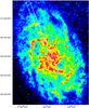 |
Fig. 1 SPIRE 250 μm map of M 33 (Xilouris et al. 2012). The rectangle delineates the 2′ × 40′ wide strip along the major axis shown in Fig. 2. Crosses mark the positions of the observed GMCs. |
Most extragalactic observations of HCN and HCO+ have so far been restricted to the nuclei of galaxies or their integrated fluxes. Exceptions are a study of HCN and HCO+ emission in the disk of M 31 by Brouillet et al. (2005), LMC observations (Chin et al. 1996, 1997, 1998; Heikkilä et al. 1999), HCN maps of seven Seyfert galaxies by Curran et al. (2001), and also HCN mapping along the major axis in 12 nearby galaxies by Gao & Solomon (2004a,b, hereafter GS04a,b). We also recommend the studies of HCN and CO and their ratios in M 51 by Kuno et al. (1995) and Schinnerer et al. (2010). The interstellar medium (ISM) of nuclear regions are often subject to particularly strong heating sources because they are often dominated by starbursts with intense UV fields heating the gas or active galactic nuclei (AGNs) with strong X-ray emission. Indeed, the HCN to HCO+ line intensity ratios are found to be systematically higher in AGN-dominated regions, such as in the central part of NGC 1068, and low in pure starburst environments, as in M 82 (e.g. Kohno et al. 2003; Imanishi et al. 2009; Krips et al. 2008, 2011).
We have targeted seven GMCs along the major axis of M 33 out to a radial distance of 4.6 kpc, using the IRAM 30 m telescope. M 33 is a spiral galaxy with Hubble type SA(s)cd located at a distance of only 840 kpc (Table 1 and Fig. 1). It is the third largest member of the Local Group (after M 31 and the Milky Way). Observations of small-scale structures in M 33 do not suffer from distance ambiguities as galactic observations do. Its small distance allows us to obtain a spatial resolution of ~ 114 pc (i.e. 28′′) at a frequency of 89 GHz (i.e. 3.3 mm) with the 30 m telescope. M 33 is seen at an intermediate inclination of i = 56°, yielding a short line-of-sight depth, which allows us to study individual cloud complexes. It is roughly ten times less massive than the Milky Way, and its overall metallicity is 12 + log O/H = 8.27, subsolar by about a factor two (Magrini et al. 2010). Therefore M 33 is particularly interesting to compare with the Milky Way, but also with the Large Magellanic Cloud that has a metallicity similar to M 33 (Hunter et al. 2007).
Using the IRAM 30 m telescope, Rosolowsky et al. (2011) (hereafter RPG11) observed four massive GMCs of more than 3 × 10⁵ M⊙ in M 33, searching for the ground-state transition HCN. They detected HCN in only two of the GMCs. The observed GMCs are under-luminous in HCN by factors between two to seven relative to their CO emission when compared to averaged values in the Milky Way.
Here, we present new, deep observations of the ground-state transitions of HCN, HCO+, 13CO, and CO towards seven GMCs in M 33 including three of the clouds observed by RPG11. All four tracers are detected in six of the GMCs. The relative weakness of HCN emission is confirmed and interpreted using models of photon-dominated regions (PDRs). To better characterize the observed GMCs, we estimated their star formation rate, total infrared luminosities, and FUV fields using a large ancillary data set compiled in the framework of the Herschel open time key project HerM33es (Kramer et al. 2010). Figure 2 shows a subset of this data set.
Basic properties of M 33.
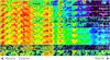 |
Fig. 2 Observed positions towards seven GMCs within a 2′ × 40′ strip along the major axis of M 33. The strip extends from 10′ south of the galactic center to 33.3′ north. The center of the strip is at 01:34:11.8 +30:50:23.4 (J2000). Circles indicate the 30 m beam size of 28′′ at 90 GHz. Panels show from top to bottom: integrated intensities of H emission (Hoopes & Walterbos 2000) 24; 70 μm emission observed with Spitzer (Tabatabaei et al. 2007); continuum emission between 100 μm and 500 μm observed with PACS and SPIRE in the framework of the HerM33es program (Kramer et al. 2010; Boquien et al. 2011; Xilouris et al. 2012); 12CO 2–1 30 m observation and H i VLA data, both taken from Gratier et al. (2010). All data are shown at their original resolutions. |
Observed intensities and complementary data.
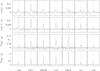 |
Fig. 3 Spectra of the ground-state transitions of HCN, HCO+, 12CO, and 13CO at the positions of seven GMCs along the major axis of M 33 (cf. Figs. 1, 2). 12CO and 13CO have been observed in position switching; HCN and HCO+ with wobbler switching. The spectra are shown on a main beam brightness temperature scale (Tmb). The velocity resolution is given by the spectrometer with the lowest resolution, i.e. WILMA, and is 5.4 km s-1 in case of 12CO and 13CO, and 6.7 km s-1 for HCN and HCO+. Center velocities are listed in Table 2. The local standard of rest (lsr) velocity displayed covers 300 km s-1. The same velocity range is used to determine the baseline (red lines), excluding the line windows determined from 12CO 1–0 (dotted lines), cf. Fig. A.1. |
2. IRAM 30 m observations
We used the IRAM 30 m telescope to perform single-pointed observations of the ground-state transitions of HCN, HCO+, 12CO, and 13CO towards seven GMCs in M 33. Observations were carried out between December 2008 and July 2012, comprising a total of 109 hours of observing time. In 2008, we used the now decommissioned A100 and B100 receivers that had a bandwidth of 500 MHz and the 1 MHz filterbank, to observe each of the four lines individually.
The bulk of the observations were carried out in 2009 employing the new eight-mixer receiver EMIR and its instantaneous bandwidth of 16 GHz in each polarization, connected to the wide-band WILMA autocorrelator backend with 2 MHz spectral resolution. This setup allowed simultaneous observation of HCN with HCO+ and 12CO with 13CO. One advantage of the simultaneous observations is that the relative intensity calibration of the lines is very accurate. The observations were carried out in wobbler switching mode using the maximum available throw of ± 120′′ and a switching frequency of two seconds. This mode ensures more stable baselines than the position-switching mode. However, the velocity resolution of about 6 km s-1 in the 3 mm band only barely resolves the spectral lines of M 33, which are typically 10–15 km s-1 wide (Gratier et al. 2010). The beam sizes are 21′′ at 115 GHz and 28′′ at 89.5 GHz, corresponding to a spatial resolution of 86 pc and 114 pc, respectively, in M 33 (cf. Table 1).
The observations of 12CO and 13CO were repeated in June and July 2012 using position-switching and the FTS spectrometers with an off position outside of the disk of M 33 to exclude the possibility of self-chopping effects in the spectra. The latter were present in some of the earlier wobbler-switched 12CO spectra. Due to the high critical density of the dense gas tracers HCN and HCO+, as well as the observed velocity gradient along the major axis of M 33 (see Table 2), we reckon that self-chopping is less probable for these lines. Please note that the 12CO data of GMC1, GMC91, and GMC26 are taken from RPG11 who also used position-switching.
All data were reduced using the GILDAS1 software package. Each scan was inspected and scans with poor baselines or unreasonably high rms values were rejected. Before averaging, linear baselines were fitted and removed. The data were regridded to a common velocity resolution. Spectra were converted from the  to the Tmb scale by multiplying with the ratio of forward efficiency (Feff = 95%) to main beam efficiency (Beff = 81%), taken to be constant for the observed 3 mm lines. The reduced spectra are shown in Fig. 3.
Integrated intensities were extracted from the spectra on a Tmb scale by summing all channels inside a velocity range around each particular line. The velocity range was determined by eye for each position from the full width to zero intensity (FWZI) of the 12CO 1–0 line and is marked in Fig. 3. We determined σ uncertainties of the integrated intensities by measuring the baseline rms ( ) in a 300 km s-1 window centered on the particular line using the corresponding 12CO 1–0 FWZI as baseline window and using
  with the number of channels N and the channel width Δvres. In case the 1σ value is higher than the typical 10% calibration error of the IRAM 30 m, the former is used to estimate the observational error for the following analysis. If the integrated intensities are lower than 3σ, we use this value as an upper limit. Table 2 lists the observed intensities, intensity ratios, and further ancillary data. For details on the latter see Appendix C. Error estimates are given in parentheses after the integrated intensities in Table 2.
3. GMCs: selection of positions and properties
Motivated by the HerM33es project, the GMCs were selected to lie within a 2′ × 40′ wide strip along the major axis of M 33 shown in Figs. 1 and 2 at a range of galacto-centric distances of up to 4.6 kpc. Three of the GMCs (GMC1, GMC26, GMC91) belong to the sample of CO-bright clouds studied by RPG11 in search of HCN emission. We added four other GMCs (no6, no3, no1, no2) to increase the range of studied galacto-centric radii, as well as physical conditions.
Table 2 lists their observed properties and Appendix C describes in detail how they were derived. The masses of the molecular gas traced by CO, calculated using XCO-factors derived individually for every cloud as a function of integrated CO 1–0 intensities and total IR luminosity (cf. Appendix C.4), vary by a factor 130 between 0.1 × 10⁵ (GMC no2) and 13 × 105 M⊙ (GMC1). The SFRs vary by more than a factor 50 and the far ultraviolet (FUV) field strengths by a factor larger than 20. The GMC near the nucleus, GMC1, is the most massive and shows the strongest SFR, as well as the highest FUV flux, while GMC no2 at 4.6 kpc radial distance is the least massive in molecular mass and shows only weak activity.
LTE column densities from the stacked spectra.
Individual areas of the strip have been mapped in [C ii] and other FIR lines in the framework of the HerM33es project, which will yield additional insight into the properties of the ISM of M 33. In the first papers on [C ii], we focused on the H ii region BCLMP 302 (Mookerjea et al. 2011) which is associated with GMC no3, and on BCLMP 691 (Braine et al., in prep.), which lies near GMC no1.
Gratier et al. (2012) identified over three hundred 12CO 2–1 clumps in M 33 and present a detailed view of each individual clump in Hff, 8 μm, 24 μm, and FUV, together with the corresponding HI and 12CO 2–1 spectra and further complementary data. The seven GMCs discussed here are among the identified clumps. In Table 2 we give the corresponding clump numbers.
4. Observed line ratios
4.1. Spectra at individual positions: HCO+ and HCN
HCO+ is detected at six positions with 6 to 12 mK peak temperatures and with good signal-to-noise ratios of at least seven; position no2 has not been detected. HCN emission is detected at the same six positions with signal-to-noise ratios of four and better; position no2 is but tentatively detected at a signal-to-noise ratio of 3.5. The HCO+/HCN ratio of line integrated intensities of positions where both molecules are detected varies between 1.1 and 2.5 (Table 2). Below, we compare the observed ratios in detail with ratios found in the Milky Way and in other galaxies. Although the integrated intensities we find for GMC26, GMC1, and GMC91 differ up to a factor of two from the values and upper limits given in RPG11 for the same positions, they are consistent within 3σ of the baseline rms of the observations from RPG11. We attribute the discrepancies to baseline problems of the RPG11 data.
4.2. Spectra at individual positions: 12CO and 13CO
Emission from 12CO and 13CO is detected at all seven positions, though varying by a factor of more than 15 between GMC no2 and GMC91. The ratio of line integrated 12CO vs. 13CO intensities varies between 9 for GMC no1 and 15 for GMC no6. In Fig. A.1 we show the 12CO and 13CO spectra at a high resolution of 1 km s-1. The resolved line shapes are Gaussian and the corresponding FWHMs are given in Table 2.
4.3. Stacked spectra
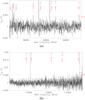 |
Fig. 4 a) Stacked spectrum of all data taken in the frequency range between 87.2 and 90.8 GHz. The red dashed line denotes the 3σ value average over the entire baseline. The HCN and HCO+ lines are not shown up to their maximum peak temperature. b) Stacked spectrum of the wobbler switched data taken in the frequency range between 108.1 and 115.5 GHz. The average 3σ value is shown as red dashed line. The baseline noise increases with frequency because of the increasing atmospheric opacity. C18O, C17O, and CN are marked but not detected. The 12CO and 13CO lines are not shown up to their maximum peak temperature. |
Stacking of all spectra allows improvement on the signal-to-noise ratios and detection of faint lines. Figure 4(a) shows the stacked spectrum of all data taken near 89 GHz. It was created by shifting all spectra in frequency such that the emission lines align in frequency. Individual spectra were weighted by integration time. In addition to the lines of HCN and HCO+, the resulting spectrum shows detections of CCH and HNC 1–0. The average baseline rms is 0.27 mK at 5.4 km s-1 resolution. HOC+ is tentatively detected with an upper limit of 19 mK km s-1, resulting in a lower limit to the HCO+/HOC+ ratio of 5.8.
The stacked spectrum centered on 112 GHz (Fig. 4(b)) does not show additional detections other than 13CO and 12COeven after additional smoothing of the velocity resolution. Table 3 lists the integrated intensities and upper limits of all detected transitions in the stacked spectrum, as well as their corresponding LTE column densities and abundances, derived as explained in Appendix D.
4.4. Comparison with other sources
4.4.1. HCO+/CO vs. HCN/CO
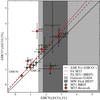 |
Fig. 5 Ratios of integrated intensities HCO+/CO vs. HCN/CO for M 33 (red points: this work) and for M 31 (green points: BR05). Upper/lower limits are denoted by arrows. Linear least squares fits to data from M 33 (red solid line) and M 31 (BR05, black dashed) are shown. Both fits exclude points with upper limits. The solid black line shows the angle bisector where I(HCO+) = I(HCN). The gray shaded areas display the range of the HCN/CO found in the disk of the Milky Way (MW) by (Helfer & Blitz 1997, HE97) (darker gray) and in a sample of normal spiral galaxies (GA04b) (lighter gray). |
For the comparison of different tracers, all data were convolved to the same resolution of 28′′. We account for the different intrinsic beam sizes of the CO, HCN, and HCO+ 1–0 observations by multiplying with beam filling factors determined from the 12CO 2–1 map (Gratier et al. 2010). Figure 5 compares the HCO+/CO vs. HCN/CO line intensities ratios observed in M 33, with those observed at nine positions in the disk of the Andromeda galaxy M 31 (Brouillet et al. 2005, hereafter BR05). M 31 lies at a similar distance as M 33 of 780 kpc and had been observed with the 30 m telescope as well. Therefore, both studies obtain about the same spatial resolution of ~114 pc.
For M 33, we find HCN/CO ratios in the range of 0.4%–2.9% (mean: 1.5 ± 0.8%) and HCO+/CO ratios in 0.6%–3.5% (mean: 1.9 ± 1.0%). BR05 finds comparable values in the spiral arms of M 31: HCN/CO 0.75%–2.8% (mean: 1.7 ± 0.5%) and HCO+/CO 1.1%–3.9% (mean: 2.0 ± 0.7%). A linear least squares fit to the M 33 data results in HCO+/CO = (1.14 ± 0.15%) HCN/CO + (0.18 ± 0.14%). This is consistent within errors to the fit results obtained by BR05 for the M 31 data: HCO+/CO = 1.07% HCN/CO + 0.23%. We excluded positions with upper limits from the fit, i.e. position GMC no2.
In the Milky Way in the solar neighborhood values of HCN/CO are found between 0.7%–1.9% (mean: 1.4 ± 2%), while the Galactic plane hosts on average 2.6 ± 0.8% (Helfer & Blitz 1997). HCO+/CO values in the Galactic center range between 0.9% and 7.6% (Riquelme et al. 2010).
The HCN/CO ratios found in the LMC by Chin et al. (1998) and Heikkilä et al. (1999) lie between 3% and 6%, and are thus higher than any value found in M 33, M 31, and also M 51 where HCN/CO = 1.1%–2% in the spiral arms are reported (Kuno et al. 1995). Unlike GS04b in a sample of normal galaxies, we do not find a systematic change in the HCN/CO ratio between regions in the center of M 33, i.e. the inner ~1 kpc (here GMC1, GMC26) and regions at greater galacto-centric distances (cf. Table 2). GS04b reports that HCN/CO drops from ~10% in the centers of normal galaxies to ~1.5%–3% in their disks  4 kpc. In ULIRGs and AGNs the ratios may reach global HCN/CO values as high as 25% (GS04b and references therein). GS04b attribute these high ratios to the presence of starbursts and argue that HCN/CO may serve as a starburst indicator.
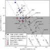 |
Fig. 6 Comparison of integrated intensities HCO+/HCN vs. HNC/HCO+ in M 33 (red filled circles and square; arrows indicate upper/lower limits) with values found in the LMC (Chin et al. 1997, 1998) (CH97, CH98; blue diamonds) and in luminous infrared galaxies compiled by Baan et al. (2008) (BA08; open symbols) and by Costagliola et al. (2011) (CO11; crosses). The dotted, dashed, and dot-dashed lines shows HNC/HCN = 1, 0.4, and 0.17 (stacked value of M 33), respectively. The gray shaded area shows the range of the observed HCO+/HCN ratios in M 31 by BR05. |
4.4.2. HCO+/HCN vs. HNC/HCO+
The HCO+/HCN ratios observed in M 33 vary between 1.1 and 2.5, while the upper limits derived for the HNC/HCO+ ratios vary between 0.2 and 0.5 (Fig. 6). The upper limit of the HNC/HCN ratio is at maximum 0.7 (GMC91), while the stacked spectrum where HNC has been detected shows a HNC/HCN ratio of 0.17 (Fig. 6).
These ratios are compared with the ratios found in luminous infrared nuclei by Baan et al. (2008) and Costagliola et al. (2011) and in H ii regions of the LMC by Chin et al. (1997, 1998) (cf. Fig.3a in Baan et al. 2010). The HCO+/HCN ratios are also compared to the range found in the disk of M 31 by BR05 (cf. Fig. 6).
The HCO+/HCN ratios, found in M 33 in the six GMCs with clear detections, lie at the upper end of the distribution of values found in LIRGs. While the starburst galaxy M 82 exhibits a higher ratio than the AGN NGC 1068 (1.6 vs. 0.9), these ratios lie within the scatter of values and their errors observed in the disk of M 33.
The HCO+/HCN ratios in M 33 lie in the overlap region between the ones found in M 31 and those found in the LMC. We find neither ratios as high as in the LMC, i.e. 3.5, nor ratios as low as in M 31, i.e. 0.51. Interestingly, all detected regions in the LMC are situated in the same parameter space as those detected in M 33.
The detection of HNC in the stacked spectrum allows us to derive an average HCO+/HNC ratio of 7.8 (Table 3) for the GMCs observed in M 33. This ratio lies at the very high end of the range of values found in any of the other samples plotted in Fig. 6.
More remarkably, the HCN/HNC value of 5.9 from the stacked spectra is higher than any from the other samples we compare with in Fig. 6. Furthermore, it is higher than ratios observed over the surface of IC 342 which are only ~1–2 (Meier & Turner 2005), higher than the ratios in a range of galaxies found by Huettemeister et al. (1995) of < 4, higher than the typical ratios of 1 observed in starburst and Seyfert galaxies (e.g. Aalto et al. 2002), and also higher than ratios of 1–3 observed in Galactic molecular complexes (Wootten et al. 1978).
This extraordinary high ratio indicates that the physics or chemistry in M 33 may be different from that of AGNs and starbursts. The dominance of strong X-ray radiation in the nuclei of AGNs or even of starbursts may be important for the differences in the line ratios, since it creates X-ray-dominated regions (XDRs) that change the chemical abundances (e.g. Meijerink & Spaans 2005).
The subsolar metallicity of M 33 may also play a role in creating such a high HCN/HNC ratio. However, the HCN/HNC ratio obtained in M 33 is significantly higher than those observed in similar low-metallicity environments, such as N159, 30 Dor in the LMC, as well as LIRS36 in the SMC, which are no higher than 3.6 (besides a lower limit of 4.7 in N27 in the SMC) (Chin et al. 1998; Heikkilä et al. 1999) and comparable to the values found in Galactic GMCs (Huettemeister et al. 1995). Therefore, a subsolar metallicity alone does not seem to be a guarantee for very high HCN/HNC ratios.
4.4.3. HCN vs. total infrared luminosity (LTIR)
The LTIR/LHCN ratios observed in M 33 (Table 2) range between 1300 and 3500 L⊙/K km s-1 pc2. These ratios lie at the upper end of the values found in Milky Way clouds (Wu et al. 2010). Normal galaxies show on average total LTIR/LHCN ratios of ~900 ± 70 L⊙/K km s-1 pc2 (Graciá-Carpio et al. 2008, GS04a,b). Higher values, in the range of ~1100–1700 L⊙/K km s-1 pc2, are found for (U-)LIRGs (Graciá-Carpio et al. 2008, GS04a,b), while the highest reported ratios are found at the extreme end of the LIRG/ULIRG distribution, as well as in high-z galaxies, and range up to ~3900 L⊙/K km s-1 pc2 (Solomon et al. 2003; Gao et al. 2007; Graciá-Carpio et al. 2008; Wu et al. 2010; García-Burillo et al. 2012). Thus the LTIR/LHCN ratios in M 33 are among the highest ratios observed.
In Sect. 6 below, we attempt to shed more light on the weak HCN emission and investigate the line ratios of CO, HCN, and HCO+ using models of photon-dominated regions that take not only the chemical network into account, but also the detailed heating and cooling processes of a cloud as well as radiative transfer.
4.4.4. 12CO/13CO line ratio
In our sample of GMCs in M 33 we find 12CO/13CO line intensity ratios between 9 and 15. There is no obvious correlation with galacto-centric distance, FUV strength, or SFR. In a study of eight GMCs in the outer disk of M 33, Braine et al. (2010) found similar ratios between 8.9 and 15.7. In the Milky Way, the isotopic ratio of 12C/13C varies between values of 80–90 in the solar neighborhood and 20 in the Galactic center (Wilson 1999). Polk et al. (1988) studied the 12CO/13CO line ratio in the Milky Way, for several large regions of the plane in comparison with the average emission from GMCs and of the centers of GMCs. They find that the average value rises from three in the centers of GMCs, to 4.5 averaged over GMCs, to 6.7 for the Galactic plane, with peaks of ~15. Their interpretation is that the higher ratios observed in the plane are caused by diffuse gas of only moderate optical thickness in 12CO. A similar interpretation may hold in M 33. The fraction of dense gas within the beam and optical depth effects may affect the ratios observed in M 33.
Ratios in the Magellanic clouds are observed by Heikkilä et al. (1999) to cover values between 5 and 18, a somewhat wider range than found in M 33. Unlike in M 33, a gradient is seen on larger scales in a set of IR-bright nearby galaxies, dropping from values of about ten in the center to values as low as two at larger radii (Tan et al. 2011). Although Aalto et al. (1995) finds variations with galacto-centric radius in some galaxies of their IR-bright sample, other galaxies exist where the 12CO/13CO stays constant with radius. They report a mean value of ~12 for the centers of most galaxies in their sample except for the most luminous mergers with ratios of 20 (see also Casoli et al. 1992).
5. Molecular abundances
Molecular abundances in M 33 and typical examples of galactic and extra-galactic sources.
We use the observed line intensities of HCO+, HCN, HNC, and C2H to estimate the molecular column densities and abundances, assuming local thermodynamic equilibrium (LTE) and optically thin emission. Details on the calculations are given Appendix D, with results shown in Table D.1. The abundances are only lower limits in case the emission of HCN and HCO+ is optically thick. In comparison with our PDR-model analysis below we find, however, that for the best-fitting models to our observations the optical depths (τ) in the centers of the lines of HCN and HCO+ are τ < 0.1, suggesting that emission is likely to be optically thin (cf. Sect. 7). In Table 4, we compare the abundances with those found in other galaxies (LMC, NGC 253, M 82, IC 342), in selected Galactic sources, the photon-dominated region Orion Bar, the dark cloud TMC-1, and a translucent cloud. The estimated column densities for the stacked values are given in Table 3.
The abundances of HCO+, HCN, and HNC found in M 33 are very similar to those found in the LMC cloud N159. The abundances derived from the stacked spectrum of M 33 agree to within 0.5 dex with those of N159. Galactic sources have values that are higher by more than an order of magnitude. The Orion Bar, for example, shows 1.8 dex to 0.8 dex higher abundances. The good agreement with the LMC may be driven by its similar metallicity of 0.3–0.5 relative to the solar metallicity (Hunter et al. 2007), which is only slightly lower on average than in M 33 (Magrini et al. 2007, 2010). However, the C2H abundance observed in M 33 and in the Orion Bar agree within 0.3 dex.
The LTE HCO+/HCN abundance ratios in M 33 range between 0.2 and 0.5 (Table D.1). Godard et al. (2010) measured an HCO+/HCN abundance ratio of 0.5 in the diffuse ISM of the Milky Way, similar to the ratio found in the solar neighborhood, and similar to the higher ratios found in M 33.
6. PDR models
6.1. Setup
To improve on the LTE analysis and to better understand why HCN is less luminous than HCO+ in M 33, we compare the observed HCO+/HCN, HCN/CO, and HCO+/CO line ratios with models of photon-dominated regions (PDRs) using the Meudon PDR code (Le Petit et al. 2006; Gonzalez Garcia et al. 2008). The line intensities of the molecules 13CO, HNC, and C2H are not modeled.
We ran a grid of models for different densities nH = 0.1, 0.5, 1, 5, 10, 50, 102 × 104 cm-3, FUV fields G0 = 10,50,100 in Habing units2, and optical extinctions Av = 2–50 mag, i.e. in steps of log Av ~ 0.2. We calculated this grid of models for a solar and a subsolar metallicity. The subsolar one is tailored to describe the metallicity in the disk of M 33. See Appendix A for a detailed description of the model setup.
6.2. Results
The modeled HCN/CO line ratio (Fig. 7, Tables E.1 and E.2) hardly varies with metallicity, nH or FUV. It varies, however strongly, with Av. After an initial drop of upto an order of magnitude for extinctions less than about 4 mag, it rises until Av ~ 20 mag and then saturates at a value that is nearly independent of any of the input parameters.
In contrast, the modeled HCO+/HCN ratio shows differences between the two metallicities for Av ≲ 10 mag. The subsolar model shows higher ratios than the solar model for a given Av, FUV field, and density. Strong FUV fields and low densities increase the ratio. At higher optical extinctions the ratios are hardly influenced by changes in metallicity, Av or FUV. This reflects the variation in HCN and HCO+ abundances. At low Av, subsolar HCN abundances are lower than solar ones by up to a factor of 0.6 dex, while HCO+ is enhanced in the subsolar models by up to 0.7 dex. Also the CO abundances show a clear dependence on metallicity. For all input parameters, its abundance in the subsolar models is ~ 0.6 dex lower than in the solar models. This directly reflects the underabundance of carbon of 0.6 dex in the subsolar models. As a result, the HCN/CO line ratio is fairly independent of metallicity.
For optical extinctions in the range of Av ≤ 8 mag, where the bulk of molecular gas in galaxies resides (Tielens 2005), the HCN/CO ratio increases with increasing densities. In general in LIRGs/ULIRGs where most of gas has higher density than in normal galaxies, the HCN/CO is also higher (GS04a,b).
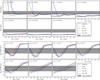 |
Fig. 7 PDR model line ratios for subsolar (solid lines) and solar metallicity (dashed lines): HCO+/HCN (top) and HCN/CO (bottom). Different colors indicate different FUV field strengths G0 = 10 (red), 50 (green), and 100 (blue). Every panel of a subfigure shows the results for one density; from left to right and top to bottom nH = 0.1, 0.5, 1, 5, 10, 50, and 102 × 104 cm-3. Gray areas mark the range of observed ratios in M 33. The dashed horizontal lines show the values from the stacked spectra. |
Best-fitting PDR models.
7. Comparison with PDR models
Figure 7 shows the range in observed intensity ratios (cf. Table 2), where the plot shows that the optical extinctions play a decisive role in determining the line ratios. High extinctions of Av > 16 mag are inconsistent with the observed HCN/CO ratios. Similarly, high densities of 105 cm-3 cannot reproduce the measured HCO+/HCN ratios. Interestingly, metallicity only plays a minor role. In general, both metallicity models allow the observed range of line ratios to be reproduced.
To quantify the agreement between the line ratios of the different models and the individual observed clouds including the stacked spectrum, we use a χ2 fit routine. To get a handle onto the errors of the best-fitting models, a Monte Carlo analysis is employed. The details on the fitting and Monte Carlo methods are given in Appendix B. Table 5 shows the input parameters Av, nH, and FUV of the best-fitting subsolar and solar metallicity models, i.e. those having the lowest χ2, for the stacked values and each observed cloud.
7.1. Stacked ratios
The best-fitting models for reproducing the stacked HCO+/HCN and HCN/CO ratios of 1.4 and 1%, respectively, that describe the averaged GMC properties are Av = 8 mag, nH = 3 × 104 cm-3, and FUV = 68 G0. Emission stems from moderately dense gas with average line-of-sight column densities of 8 mag. The beam-filling factor ΦFUV derived from ratio of the beam-averaged TIR intensity to the fitted local FUV field is ~30%; i.e., the fitted FUV field strengths are significantly higher than expected from the observations. The same holds for the beam filling factors deduced from the ratios of extinctions derived from CO and the Av of the best-fitting models, which are about ΦAv = 50%. This is not surprising, however, and indicates that emission is clumped within the 114 pc beam. From the models of the calculated grid closest to the best fit, i.e., Av = 6 and 10 mag, nH = 1 × 10⁴, and FUV = 50 G0, we find optical depths (τ) in the centers of the lines of HCN and HCO+ that lie between 0.02–0.1 and 0.07–0.1, respectively. Thus both lines are optically thin. 12CO is moderately optically thick with optical depths of τ 4–25. The line width assumed in the Meudon PDR code is ~3 km s-1 (cf. Appendix A).
7.2. Individual regions
Here, we focus on individual regions grouped by their particular HCO+/HCN ratios and thus their best-fit Av values: no6 showing a high ratio of 2.5, GMC91, no3, and no1 have intermediate ratios of 1.4–1.9 and GMC26, GMC1 having ratios of 1.1–1.2.
GMC no6
This cloud shows the highest HCO+/HCN ratio of 2.5, while at the same time the HCN/CO ratio is relatively low with 1.4 and weaker than expected from the linear fit to the M 33 data (cf. Sect. 4.4.1 and Fig. 5). GMC no6 is best fitted by subsolar models that yield a low best-fitting value for Av of ~4 mag, while the best-fitting density and FUV strength are 6 × 103 cm-3 and 40 G0, respectively. The beam-filling factor derived from Av is 1.7, indicating that emission completely fills the beam with several clouds along the line-of-sight. This cloud has the second highest star formation rate of our sample of 35.9 M⊙ Gyr-1 pc-2, and the same holds for the FUV field strength of 37.3 G0.
GMC91, no3, and no1
The line ratios of these three clouds are best described by subsolar models. The best-fitting Av are similar with 6–8 mag. So are the FUV 30–50 G0 and the densities 3 × 103 cm-3–3 × 104 cm-3, and no1 and no3 have similar SFR rates of ~13 M⊙ Gyr-1 pc-2, while no3 is a factor of four more massive than no1 with MH2 = 8 × 10⁵ M⊙. GMC91 lies at only 320 pc distance in close vicinity of GMC no3 and is only slightly more massive than the same. It is the most CO intense cloud in our sample while its HCN and HCO+ emission is relatively weak. This renders GMC91 somewhat peculiar and results in a low HCO+/CO ratio of 0.6% and, as already found by RPG11, a particularly low HCN/CO intensity ratio of 0.4% (Table 2). The HCN/CO ratio of GMC91 is much lower than the ratios observed in the disk of the Milky Way by Helfer & Blitz (1997), who find 2.6% ± 0.8% and also in the inner disks (5–10 kpc) of normal galaxies by GS04b who find 4% ± 2%. The relatively weak HCN and HCO+ emission may indicate a low fraction of dense mass in GMC91, which thus may be a rather quiescent GMC with only a low SFR. Indeed, it has the lowest star formation rate of 4 M⊙ Gyr-1 pc-2 of all observed clouds.
GMC1 and GMC26
These two clouds host the lowest observed ratios of HCO+/HCN of 1.1–1.2. Here, the solar models provide slightly better or equal fits than the subsolar models. However, since the ISM of M 33 is subsolar, here we discuss only the best fits to the subsolar models. These GMCs have similar best-fitting input parameters of Av 9–10 mag and nH ~ 104 cm-3, while the best-fitting FUV field strengths are ~30 G0 and 70 G0, respectively. However comparing their physical properties in Table 2, again, these two clouds are actually not at all alike. GMC1 is located in the very center of M 33 and is by far the most massive cloud in our sample. It is actively forming stars at a rate of 65 M⊙ Gyr-1 pc-2, the highest in our sample, and has an correspondingly high FUV field of 50.7 G0. GMC26 has much lower HCN/CO ratios, and its SFR is only 6.6 M⊙ Gyr-1 pc-2 the second lowest in the sample with exception of no2.
For all best-fitting solutions of the six individual positions we find that the modeled optical depths of HCN and HCO+ are τ ≤ 0.1, which renders emission of these lines to be likely optically thin. This also justifies the assumption of optical thin emission for the LTE analysis in Sect 5. Indeed, the PDR modeled abundances of both molecules are comparable to the ones derived from LTE (cf. Table 4 and E.2).
In conclusion, it is noteworthy to repeat that the line ratios studied here are fairly independent of the metallicity, SF activity, and FUV field strength of the parent GMC, while the optical extinction has a major influence on the modeled line ratios.
8. Summary
We present IRAM 30 m observations of the ground-state transitions of HCN, HCO+, 12CO and 13CO of seven GMCs distributed along the major axis in the disk of the nearby spiral galaxy M 33. We achieve a spatial resolution of ~114 pc at a frequency of 89 GHz.
The molecular gas masses of the target GMCs vary by a factor of ~130 between 0.1 × 10⁵ M⊙ (GMC no2) and 13 × 105 M⊙ (GMC1) and the star formation rates derived from Hα and 24 μm images vary by a factor of more than 50. The FUV field strengths show a variation of more than a factor 20. Below, we summarize the main results.
-
1.
For the six GMCs where HCO+ is detected, peakline temperatures (on the Tmb scale) vary between 6 and 12 mK. The HCO+/HCN-integrated intensity line ratios lie between 1.1 and 2.5 (on the K km s-1 scale, cf. Table 2). Similar line ratios are observed in the disk of M 31 (Brouillet et al. 2005).
-
2.
The line intensity ratios HCN/CO and HCO+/CO vary between (0.4 − 2.9)% and (0.6 − 3.5)%, respectively. The spread of ratios found in M 33 is slightly larger than in the spiral arms of M 31 (Brouillet et al. 2005, Fig 5). GMC 91 exhibits a particularly low HCN/CO ratio of 0.4%, which is much lower than values in the Galactic disk of 2.5% ± 0.6% (Helfer & Blitz 1997) or in normal galaxies with 4% ± 2% (GS04a).
-
3.
The
 luminosity ratios range between 1.3 × 10³ and 3.5 × 10³ and are situated at the very high end of ratios found by Wu et al. (2010) in molecular clouds of the Milky Way and LIRGs/ULIRGs. This shows that HCN emission in comparison to the LTIR in M 33 particularly weak.
 -
4.
Stacking of all spectra taken at the seven GMC positions leads to 3σ detections of CCH and HNC. The HCN/HNC ratio of 5.8 is remarkable high. It is higher than values found in the LMC (Chin et al. 1997, 1998), in IC 342 (Meier & Turner 2005), in samples of LIRGs/ULIRGs (Baan et al. 2008; Costagliola et al. 2011), in starburst and Seyfert galaxies (e.g. Aalto et al. 2002), and in Galactic molecular complexes Wootten et al. (1978), where all together no values higher than three are reported.
-
5.
The HCO+, HCN, HNC abundances, derived assuming LTE, agree with those of the LMC cloud N159 within 0.5 dex. In contrast, the Orion Bar, a Galactic massive star-forming region, shows significantly higher abundances of all three tracers by 0.8 dex to 1.8 dex. These striking differences may reflect the factor two subsolar metallicities of both the LMC and M 33.
-
6.
Employing the Meudon PDR code to model photon-dominated regions we investigated the influence of the metallicity on the abundances and emission of HCN and HCO+. For a range of optical extinctions, volume densities, and FUV radiation field strengths, we derived two sets of models with different metallicity, one reflecting the abundances in the Orion nebula by Simón-Díaz & Stasińska (2011), the other the average subsolar metallicity of M 33 (Magrini et al. 2010). Both sets of models are able to describe the observed range of HCO+/HCN and HCN/CO line ratios reasonably well (χ2 < 3.4). Therefore, changes in metallicity do not need to be invoked to describe the observed line ratios. The observations are described by subsolar models with optical extinctions between 4 mag and 10 mag and moderate densities of <3 × 104 cm-3, with little influence by the FUV field strength. The optical extinction has a pronounced influence on the modeled ratios, while FUV field, metallicity and even density only play minor roles. The modeled lines of HCN and HCO+ of the best-fitting models are found to be optically thin with optical depths τ ≤ 0.1.
Online material
Appendix A: PDR Model setup
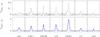 |
Fig. A.1 12CO and 13CO 1-0 spectra at the seven selected GMC positions at high-velocity resolution of 1 km s-1. The 12CO spectra of positions GMC91, GMC26 and GMC1 are taken from RPG11. The blue lines overplotted on the 12CO spectra show the Gaussian line fits used to deduce the FWHM of the lines which are listed in Table 2. |
We use the Meudon PDR code (Le Petit et al. 2006; Gonzalez Garcia et al. 2008), which solves the thermal balance, chemical network, detailed balance, and radiative transfer of a plane-parallel slab of optical extinction Av and constant density nH illuminated from both sides by an FUV field of intensity G0. The modeled line widths are calculated by the Meudon code via the Doppler broadening of the gas due to the kinetic temperature and the turbulent velocity of the gas. The latter dominates the line widths and is an input parameter to the Meudon code. We use the default value of the Meudon code which, expressed in terms of the FWHM of the velocity distribution, is (Δ v)FWHM ~ 3 km s-1. This is slightly lower than the observed line widths that are in the range of 4–11 km s-1. We also used the defaults for additional input parameters (e.g. the cosmic-ray ionization rate and size distribution of dust grains).
Initial Abundances used in the PDR models.
The grid of models has been calculated for volume densities nH = 0.1, 0.5, 1, 5, 10, 50, 102 × 104 cm-3, FUV field strengths G0 = 10, 50, 100 in Habing units, and optical extinctions Av = 2–50 mag, i.e. in steps of log Av ~ 0.2.
The input range of FUV fields is motivated by the range of FUV fields derived from the TIR in the six observed clouds which vary between G0 = 11.3 and 50.7, excluding position no2 with a very low G0 of 2.5 (cf. Table 2). We add models of G0 = 100 to cover possible higher local radiation fields. The values of AV range from those found in translucent clouds with 2 mag to extinctions of 50 mag typically found in resolved Galactic high-mass star-forming clouds. The densities cover values found in a typical molecular cloud, covering the critical densities of the observed tracers and transitions.
We calculated this grid of models for solar and subsolar metallicities. Table A.1 shows the abundances measured in M 33 and in the Orion nebula which we use as initial abundances for our PDR models. The abundances of the sun are listed for comparison. For the “solar” metallicity model, we adopt the abundances of O, C, N, S, Fe measured in the H ii region of the Orion nebula by Simón-Díaz & Stasińska (2011). The heavy elements S and Fe are depleted to dust grains with respect to the abundances found in the solar photosphere.
For the subsolar metallicity PDR model, we adopt the averaged O, N, and S abundances measured in M 33 from Magrini et al. (2010) who targeted 33 H ii regions between 1 and 8 kpc galacto-centric distance. The carbon gas-phase abundance has not been measured in M 33. We estimate it using the metallicity dependence of the C/O ratio described by (Henry et al. 2000). To derive the Fe abundance, we scale the solar Fe/O ratio by the subsolar O metallicity of M 33.
Appendix B: Chi-squared fitting and Monte Carlo analysis
To quantitatively compare the modeled and observed line ratios we calculate the summed squared residuals weighted by the observational errors between the modeled and observed line ratios HCO+/HCN and HCN/CO, for every model and for each observed cloud as  (B.1)where σ is the observational error of the line ratios deduced from the errors of the line intensities, cf. Sect. 2. We normalize the χ2 by dividing by N = 2, the number of independent observed line ratios. The minimum χ2 gives the best-fitting model.
To get a handle on the errors of the best-fitting models, we employ a Monte Carlo simulation. We assume that the measured ratios and their errors follow a Gaussian distribution with an expected value equal to the ratio and a variance equal to σ2.
We generate 5000 sets of HCN/CO and HCO+/HCN ratios drawn randomly from their Gaussian parent distribution. For every set we calculate a χ2 as explained above and deduce the best fits. From all best fits of all sets we derive the mean and the standard deviation of the input parameters: nH, Av, FUV, and χ2 (Table 5).
Appendix C: GMC properties
For comparison we derived complementary properties, the star formation rate, the FUV field, the XCO factor, the masses of the molecular and atomic material, and the optical extinction within the beam at the observed positions (Table 2). Below, we explain in detail how these values have been derived. All errors are calculated using Gaussian error propagation. The particular uncertainties of individual measurements used to derive the complementary quantities are given below.
C.1. Star formation rate (SFR) and total infrared luminosity (TIR)
To obtain an extinction free tracer of the SFR we combine the 24 μm (Tabatabaei et al. 2007) and H luminosity (Hoopes & Walterbos 2000) using (Calzetti et al. 2007). We assume errors of 7% for 24 μm (Spitzer Observers Manual v8.0) and 15% for H.
Another measure of the SFR is the total infrared luminosity (LTIR) emitted between 1 μm and 1 mm. We estimate it by adding the measured brightnesses at 24, 70, 100, 160, 250, 350, 500 μm, in W kpc-2 weighted by the factors determined by Boquien et al. (2011). We convert the determined brightnesses to luminosities corresponding to the 28′′ beam by multiplying with the beam size in kpc-2. The errors on the derived TIR are the σ values of the fits given by Boquien et al. (2011).
C.2. Molecular line luminosities
We calculate the molecular line luminosities  and
and  in units of K km s-1 pc2 by multiplying the integrated line intensities with the beam size in pc2, i.e. 1.5 × 10⁴ pc2. Errors follow from the measurement uncertainties given in Table 2.
C.3. FUV flux G0
The FUV flux G0 impinging on the dusty cloud surfaces can be estimated from the emitted total infrared intensity assuming that all FUV photons are absorbed by the dust. We use G0 = 4π 0.5 LTIR (cf. e.g. Mookerjea et al. 2011) with G0 in units of the Habing field 1.6 10-3 erg s-1 cm2 (Habing 1968) and the TIR intensity in units of erg s-1 cm-2 sr-1. Errors follow directly from the errors on LTIR. The FUV flux that we use to compare with values deduced from the stacked spectrum is the average FUV flux of all individual clouds, i.e. 21.6 ± 0.7 G0.
C.4. XCO factor and atomic and molecular gas mass
To derive the masses of the molecular gas we first convert the CO 1–0 integrated intensities into H2 column densities (NH2) via NH2 = ICOXCO. We assume that the conversion factor XCO (cf. Table 2) is a function of total infrared luminosity as found by Israel (1997) for a sample of low-metallicity environments in the LMC and SMC and for two clouds in M 33 (cf. Leroy et al. 2011).
Israel (1997) derived NH2 for CO clouds in the LMC, the SMC, and other low-metallicity galaxies from their far-infrared surface brightness and H i column densities. He finds local XCO values up to a magnitude higher than the widely used Galactic value of 2 × 10²⁰ (K km s-1)-1 cm-2 (e.g. Dame et al. 2001). In particular he studies the two bright H ii regions NGC 604 and NGC 595 in M 33, for which he derives X-factors of 22 × 1020 (K km s-1)-1 cm-2 and 12 1020 (K km s-1)-1 cm-2. Israel (1997) further finds a correlation between XCO and the TIR-flux. For NGC 604 we find a TIR luminosity of 27.18 and 7.82 × 10⁶ L⊙ for NGC 595 (cf. Sec. C.1). We estimate the local XCO for our seven clouds from their TIR by using the mean of the XCO/LTIR ratio of NGC 604 and NGC 595 as a conversion factor, i.e. XCO = 1.17 × 10²⁰ 10-6 L⊙LTIR. The derived X-factors vary between 7 and 1.5 in units of 1020 (K km s-1)-1 cm-2 for the six positions with HCN and HCO+ detections (Table 2). Gratier et al. (2010) assume a constant X-factor of 4 × 10²⁰ (K km s-1)-1 cm-2.
The mass of the molecular gas MH2 is estimated from the intensity of the 12CO 1–0 line using the XCO-factor derived in the previous section and MH2 = 2 × 1.36 NH2 mp A with the proton mass mp, the beam size A. The factor two accounts for the two protons of molecular hydrogen and 1.36 includes the contribution of heavy elements to the total mass. Errors follow from the measurement uncertainty of 12CO given in Table 2.
The mass of the atomic gas is estimated from the intensity of the H i line via the column density (Rohlfs & Wilson 2000) assuming optically thin emission. The atomic gas mass is calculated with the same formula as for the molecular mass without the factor two accounting for the two protons in H2. Errors assume a 15% calibration error on the HI data.
C.5. Optical extinction Av
As shown by Bohlin et al. (1978) a correlation between the amount of hydrogen atom column density N(H i + H2) and the color excess exists; they estimate a conversion factor of ⟨ N(H i + H2) ⟩ /E(B − V) = 5.8 × 10²¹ atoms cm-2 mag-1. The color excess and the optical extinction Av are also linked. Bohlin et al. (1978) give a value for the interstellar average of R = Av/E(B − V) = 3.1. Using the two conversion formula and the values for and NH2, derived as explained in the previous section, we calculate an estimate of the optical extinction for the observed clouds per beam. For clouds not filling the 115 pc beam, local extinctions may be higher. The errors given for Av (cf. Table 2) include the errors of N(H i) and N(H2). We estimate the Av for the stacked spectra by averaging the values of the individual positions, i.e. 4.2 ± 1.9 mag.
Appendix D: LTE column densities
LTE column densities at the individual positions.
We estimate column densities from the integrated intensities, assuming LTE and optically thin emission: ![\appendix \setcounter{section}{4} \begin{equation} \label{formula:coldens} N = \frac{3h}{8 \pi^3 \mu^2} \frac{Z}{J} \frac{\exp(\frac{h \nu}{k T_{\rm ex}})}{\left[1 - \exp\left(-\frac{h \nu}{k T_{\rm ex}}\right)\right]} (\mathcal{J}_{\nu}(T_{\rm ex}) - \mathcal{J}_{\nu}(T_{\rm BG}))^{-1} \int{T_{\rm mb} {\rm d} \nu} , \end{equation}](/articles/aa/full_html/2013/01/aa19436-12/aa19436-12-eq182.png) (D.1)with:
(D.1)with:  (D.2)where Z the partition function, J the rotational quantum number of the upper level, μ the dipole moment, Tex the excitation temperature, TBG the temperature of the cosmic background, and Tmb the main beam temperature of the specific line. Table D.2 lists frequency, μ, Eu/kb, and the critical densities of the observed transitions. The partition function is taken from the “Cologne Database for Molecular Spectroscopy” (CDMS) (Müller et al. 2001, 2005). The value of Z depends on Tex. The CDMS lists values for discrete temperatures in the range from 2.75 to 500 K for every molecule. We use these values to interpolate Z for the excitation temperature we adopt at a specific position.
Molecule parameters.
To estimate the excitation temperature, we derive the dust temperature, assuming that Tex, the kinetic temperature Tkin, and the dust temperature Tdust are coupled and equal. To estimate Tdust we obtain the dust SEDs for all our pointings from the Herschel and Spitzer observations at 500, 350, 250, 160, 100, and 24 μm 28′′ resolution and fit two-component graybody models to the data. Each component is described by Sν = B(ν,T)τν = B(ν,T)κνMd/D2, assuming optically thin emission, with the flux Sν, the Planck function Bν, the opacity τν, the dust mass Md, the distance D, and the dust absorption coefficient κν = 0.4(ν/(250 GHz))β cm2 g-1 (Kruegel & Siebenmorgen 1994; Krügel 2003), β is the dust emissivity index assumed to be 1.5.
Tdust is found to vary only slightly, between 20 K in the northernmost position observed, GMC no2, and 26 K in the nuclear
GMC, GMC1 (cf. Table D.1). We assume that Tex equals the temperature of the cold dust component.
The CCH 1–0 transition is split into six hyperfine components. In the stacked spectrum, we detected the 3/2–1/2, 2–1 transition, which is the strongest one. To determine LTE column densities of CCH, we estimate the total integrated intensity of the CCH 1–0 line including all hyperfine components by dividing the result of a Gaussian fit to the detected component by its relative strength, i.e. 0.416 (Padovani et al. 2009).
The column density of H2 is estimated from 13CO 1–0, assuming a 12CO/13CO abundance ratio of 60 as typically found in the Milky Way (Langer & Penzias 1993) and a H2/CO abundance ratio of 8.5 × 10⁻⁵, also found for the Milky Way (Frerking et al. 1982). From this we derive the relative abundances of the different species with respect to NH2. The derived column densities, as well as the relative abundances, are given in Table D.1 for individual clouds and in Table 3 for the stacked spectra. For comparison we give in Table D.1 the values of NH2 that we derive from the 12CO 1–0 lines using the individual XCO-factors derived for every cloud (see above). After comparing both methods to obtain the column density of H2, we find that the results are consistent within a factor of 2.5 excluding position no2. The values of NH2 for the stacked values in Table 3 are deduced using an average over the individual XCO factor of the observed GMCs of 3.0 × 10²⁰ (K km s-1)-1 cm-2.
Appendix E: PDR Model results
The modeled abundances and intensity ratios of the ground-state transition of HCN, HCO, and 12CO using the Meudon PDR code for subsolar and solar metallicities are shown in Tables E.1 and E.2. Both tables are subdivided in three blocks one for each modeled radiation field of G0 = 10,50,and 100 in Habing units, which illuminates the modeled clouds from both sides. The other two input parameters that have been varied are the density with values of nH = 0.1, 0.5, 1, 5, 10, 50, 102 × 104 cm-3 and the optical extinctions with values of Av = 2, 4, 6, 10, 16, 26, 40, and 50 mag.
Results of the PDR models with solar metallicities.
Habing units correspond to an average interstellar radiation field (ISRF) between 6 eV ≤ hν ≤ 13.6 eV of 1.6 × 10⁻³ erg cm-2 s-1 (Habing 1968). Another unit that is frequently used is the Draine unit of the local average ISRF, which is 1.7 × G0 in Habing units.
Acknowledgments
P.G. is supported by the French Agence Nationale de la Recherche grant ANR-09-BLAN-0231-01 as part of the SCHISM project.
References
- Aalto, S., Booth, R. S., Black, J. H., & Johansson, L. E. B. 1995, A&A, 300, 369 [NASA ADS] [Google Scholar]
- Aalto, S., Polatidis, A. G., Hüttemeister, S., & Curran, S. J. 2002, A&A, 381, 783 [NASA ADS] [CrossRef] [EDP Sciences] [Google Scholar]
- Asplund, M., Grevesse, N., Sauval, A. J., & Scott, P. 2009, ARA&A, 47, 481 [NASA ADS] [CrossRef] [Google Scholar]
- Baan, W. A., Henkel, C., Loenen, A. F., Baudry, A., & Wiklind, T. 2008, A&A, 477, 747 [NASA ADS] [CrossRef] [EDP Sciences] [Google Scholar]
- Baan, W. A., Loenen, A. F., & Spaans, M. 2010, A&A, 516, A40 [NASA ADS] [CrossRef] [EDP Sciences] [Google Scholar]
- Bohlin, R. C., Savage, B. D., & Drake, J. F. 1978, ApJ, 224, 132 [NASA ADS] [CrossRef] [Google Scholar]
- Boquien, M., Calzetti, D., Combes, F., et al. 2011, AJ, 142, 111 [NASA ADS] [CrossRef] [Google Scholar]
- Braine, J., Gratier, P., Kramer, C., et al. 2010, A&A, 520, A107 [NASA ADS] [CrossRef] [EDP Sciences] [Google Scholar]
- Brouillet, N., Muller, S., Herpin, F., Braine, J., & Jacq, T. 2005, A&A, 429, 153 [NASA ADS] [CrossRef] [EDP Sciences] [Google Scholar]
- Calzetti, D., Kennicutt, R. C., Engelbracht, C. W., et al. 2007, ApJ, 666, 870 [NASA ADS] [CrossRef] [Google Scholar]
- Casoli, F., Dupraz, C., & Combes, F. 1992, A&A, 264, 55 [NASA ADS] [Google Scholar]
- Chin, Y.-N., Henkel, C., Millar, T. J., Whiteoak, J. B., & Mauersberger, R. 1996, A&A, 312, L33 [NASA ADS] [Google Scholar]
- Chin, Y.-N., Henkel, C., Whiteoak, J. B., et al. 1997, A&A, 317, 548 [NASA ADS] [Google Scholar]
- Chin, Y.-N., Henkel, C., Millar, T. J., Whiteoak, J. B., & Marx-Zimmer, M. 1998, A&A, 330, 901 [NASA ADS] [Google Scholar]
- Costagliola, F., Aalto, S., Rodriguez, M. I., et al. 2011, A&A, 528, A30 [NASA ADS] [CrossRef] [EDP Sciences] [Google Scholar]
- Curran, S. J., Polatidis, A. G., Aalto, S., & Booth, R. S. 2001, A&A, 368, 824 [NASA ADS] [CrossRef] [EDP Sciences] [Google Scholar]
- Dame, T. M., Hartmann, D., & Thaddeus, P. 2001, ApJ, 547, 792 [NASA ADS] [CrossRef] [Google Scholar]
- de Vaucouleurs, G., de Vaucouleurs, A., Corwin, Jr., H. G., et al. 1991, Third Reference Catalogue of Bright Galaxies (Springer) [Google Scholar]
- Freedman, W. L., Wilson, C. D., & Madore, B. F. 1991, ApJ, 372, 455 [NASA ADS] [CrossRef] [Google Scholar]
- Frerking, M. A., Langer, W. D., & Wilson, R. W. 1982, ApJ, 262, 590 [NASA ADS] [CrossRef] [Google Scholar]
- Galleti, S., Bellazzini, M., & Ferraro, F. R. 2004, A&A, 423, 925 [NASA ADS] [CrossRef] [EDP Sciences] [Google Scholar]
- Gao, Y., & Solomon, P. M. 2004a, ApJS, 152, 63 [NASA ADS] [CrossRef] [Google Scholar]
- Gao, Y., & Solomon, P. M. 2004b, ApJ, 606, 271 [NASA ADS] [CrossRef] [Google Scholar]
- Gao, Y., Carilli, C. L., Solomon, P. M., & Van den Bout, P. A. 2007, ApJ, 660, L93 [NASA ADS] [CrossRef] [Google Scholar]
- García-Burillo, S., Usero, A., Alonso-Herrero, A., et al. 2012, A&A, 539, A8 [NASA ADS] [CrossRef] [EDP Sciences] [Google Scholar]
- Godard, B., Falgarone, E., Gerin, M., Hily-Blant, P., & de Luca, M. 2010, A&A, 520, A20 [NASA ADS] [CrossRef] [EDP Sciences] [Google Scholar]
- Gonzalez Garcia, M., Le Bourlot, J., Le Petit, F., & Roueff, E. 2008, A&A, 485, 127 [NASA ADS] [CrossRef] [EDP Sciences] [Google Scholar]
- Graciá-Carpio, J., García-Burillo, S., & Planesas, P. 2008, Ap&SS, 313, 331 [NASA ADS] [CrossRef] [Google Scholar]
- Gratier, P., Braine, J., Rodriguez-Fernandez, N. J., et al. 2010, A&A, 522, A3 [NASA ADS] [CrossRef] [EDP Sciences] [Google Scholar]
- Gratier, P., Braine, J., Rodriguez-Fernandez, N. J., et al. 2012, A&A, 544, A55 [NASA ADS] [CrossRef] [EDP Sciences] [Google Scholar]
- Habing, H. J. 1968, Bull. Astron. Inst. Netherlands, 19, 421 [Google Scholar]
- Heikkilä, A., Johansson, L. E. B., & Olofsson, H. 1999, A&A, 344, 817 [NASA ADS] [Google Scholar]
- Helfer, T. T., & Blitz, L. 1997, ApJ, 478, 233 [NASA ADS] [CrossRef] [Google Scholar]
- Henry, R. B. C., Edmunds, M. G., & Köppen, J. 2000, ApJ, 541, 660 [NASA ADS] [CrossRef] [Google Scholar]
- Hogerheijde, M. R., & Sandell, G. 2000, ApJ, 534, 880 [NASA ADS] [CrossRef] [Google Scholar]
- Hoopes, C. G., & Walterbos, R. A. M. 2000, ApJ, 541, 597 [NASA ADS] [CrossRef] [Google Scholar]
- Huettemeister, S., Henkel, C., Mauersberger, R., et al. 1995, A&A, 295, 571 [NASA ADS] [Google Scholar]
- Hunter, I., Dufton, P. L., Smartt, S. J., et al. 2007, A&A, 466, 277 [NASA ADS] [CrossRef] [EDP Sciences] [Google Scholar]
- Imanishi, M., Nakanishi, K., Tamura, Y., & Peng, C. 2009, AJ, 137, 3581 [Google Scholar]
- Israel, F. P. 1997, A&A, 328, 471 [NASA ADS] [Google Scholar]
- Johansson, L. E. B., Olofsson, H., Hjalmarson, A., Gredel, R., & Black, J. H. 1994, A&A, 291, 89 [NASA ADS] [Google Scholar]
- Kohno, K., Ishizuki, S., Matsushita, S., Vila-Vilaró, B., & Kawabe, R. 2003, PASJ, 55, L1 [NASA ADS] [CrossRef] [Google Scholar]
- Kramer, C., Buchbender, C., Xilouris, E. M., et al. 2010, A&A, 518, L67 [NASA ADS] [CrossRef] [EDP Sciences] [Google Scholar]
- Krips, M., Neri, R., García-Burillo, S., et al. 2008, ApJ, 677, 262 [NASA ADS] [CrossRef] [Google Scholar]
- Krips, M., Martín, S., Eckart, A., et al. 2011, ApJ, 736, 37 [NASA ADS] [CrossRef] [Google Scholar]
- Kruegel, E., & Siebenmorgen, R. 1994, A&A, 288, 929 [NASA ADS] [Google Scholar]
- Krügel, E. 2003, The physics of interstellar dust (Bristol, UK: The Institute of Physics) [Google Scholar]
- Kuno, N., Nakai, N., Handa, T., & Sofue, Y. 1995, PASJ, 47, 745 [NASA ADS] [Google Scholar]
- Langer, W. D., & Penzias, A. A. 1993, ApJ, 408, 539 [NASA ADS] [CrossRef] [Google Scholar]
- Le Petit, F., Nehmé, C., Le Bourlot, J., & Roueff, E. 2006, ApJS, 164, 506 [NASA ADS] [CrossRef] [EDP Sciences] [Google Scholar]
- Leroy, A. K., Bolatto, A., Gordon, K., et al. 2011, ApJ, 737, 12 [NASA ADS] [CrossRef] [Google Scholar]
- Liu, L., & Gao, Y. 2012, Science China Physics, Mechanics and Astronomy, 55, 347 [NASA ADS] [Google Scholar]
- López-Sepulcre, A., Cesaroni, R., & Walmsley, C. M. 2010, A&A, 517, A66 [NASA ADS] [CrossRef] [EDP Sciences] [Google Scholar]
- Magrini, L., Vílchez, J. M., Mampaso, A., Corradi, R. L. M., & Leisy, P. 2007, A&A, 470, 865 [NASA ADS] [CrossRef] [EDP Sciences] [Google Scholar]
- Magrini, L., Stanghellini, L., Corbelli, E., Galli, D., & Villaver, E. 2010, A&A, 512, A63 [NASA ADS] [CrossRef] [EDP Sciences] [Google Scholar]
- Martín, S., Mauersberger, R., Martín-Pintado, J., Henkel, C., & García-Burillo, S. 2006, ApJS, 164, 450 [NASA ADS] [CrossRef] [Google Scholar]
- Meier, D. S., & Turner, J. L. 2005, ApJ, 618, 259 [NASA ADS] [CrossRef] [Google Scholar]
- Meijerink, R., & Spaans, M. 2005, A&A, 436, 397 [NASA ADS] [CrossRef] [EDP Sciences] [Google Scholar]
- Mookerjea, B., Kramer, C., Buchbender, C., et al. 2011, A&A, 532, A152 [NASA ADS] [CrossRef] [EDP Sciences] [Google Scholar]
- Müller, H. S. P., Thorwirth, S., Roth, D. A., & Winnewisser, G. 2001, A&A, 370, L49 [NASA ADS] [CrossRef] [EDP Sciences] [Google Scholar]
- Müller, H. S. P., Schlöder, F., Stutzki, J., & Winnewisser, G. 2005, J. Mol. Struct., 742, 215 [NASA ADS] [CrossRef] [Google Scholar]
- Omont, A. 2007, Rep. Progress Phys., 70, 1099 [Google Scholar]
- Padovani, M., Walmsley, C. M., Tafalla, M., Galli, D., & Müller, H. S. P. 2009, A&A, 505, 1199 [NASA ADS] [CrossRef] [EDP Sciences] [Google Scholar]
- Paturel, G., Petit, C., Prugniel, P., et al. 2003, A&A, 412, 45 [NASA ADS] [CrossRef] [EDP Sciences] [Google Scholar]
- Polk, K. S., Knapp, G. R., Stark, A. A., & Wilson, R. W. 1988, ApJ, 332, 432 [NASA ADS] [CrossRef] [Google Scholar]
- Regan, M. W., & Vogel, S. N. 1994, ApJ, 434, 536 [NASA ADS] [CrossRef] [Google Scholar]
- Riquelme, D., Bronfman, L., Mauersberger, R., May, J., & Wilson, T. L. 2010, A&A, 523, A45 [NASA ADS] [CrossRef] [EDP Sciences] [Google Scholar]
- Rohlfs, K., & Wilson, T. L. 2000, Tools of Radio Astronomy (New York: Springer) [Google Scholar]
- Rosolowsky, E., Pineda, J. E., & Gao, Y. 2011, MNRAS, 415, 1977 [NASA ADS] [CrossRef] [Google Scholar]
- Schinnerer, E., Weiß, A., Aalto, S., & Scoville, N. Z. 2010, ApJ, 719, 1588 [NASA ADS] [CrossRef] [Google Scholar]
- Simón-Díaz, S., & Stasińska, G. 2011, A&A, 526, A48 [NASA ADS] [CrossRef] [EDP Sciences] [Google Scholar]
- Solomon, P., Van den Bout, P., Carilli, C., & Guelin, M. 2003, Nature, 426, 636 [NASA ADS] [CrossRef] [PubMed] [Google Scholar]
- Tabatabaei, F. S., Beck, R., Krause, M., et al. 2007, A&A, 466, 509 [NASA ADS] [CrossRef] [EDP Sciences] [Google Scholar]
- Tan, Q.-H., Gao, Y., Zhang, Z.-Y., & Xia, X.-Y. 2011, Res. Astron. Astrophys., 11, 787 [NASA ADS] [CrossRef] [Google Scholar]
- Tielens, A. 2005, The Physics and Chemistry of the Interstellar Medium (Cambridge University Press) [Google Scholar]
- Turner, B. E. 2000, ApJ, 542, 837 [NASA ADS] [CrossRef] [Google Scholar]
- Wilson, T. L. 1999, Rep. Progress Phys., 62, 143 [NASA ADS] [CrossRef] [Google Scholar]
- Wootten, A., Evans, II, N. J., Snell, R., & van den Bout, P. 1978, ApJ, 225, L143 [NASA ADS] [CrossRef] [Google Scholar]
- Wu, J., Evans, II, N. J., Gao, Y., et al. 2005, ApJ, 635, L173 [NASA ADS] [CrossRef] [Google Scholar]
- Wu, J., Evans, II, N. J., Shirley, Y. L., & Knez, C. 2010, ApJS, 188, 313 [NASA ADS] [CrossRef] [Google Scholar]
- Xilouris, E. M., Tabatabaei, F. S., Boquien, M., et al. 2012, A&A, 543, A74 [NASA ADS] [CrossRef] [EDP Sciences] [Google Scholar]
- Zaritsky, D., Elston, R., & Hill, J. M. 1989, AJ, 97, 97 [NASA ADS] [CrossRef] [Google Scholar]
All Tables
Molecular abundances in M 33 and typical examples of galactic and extra-galactic sources.
All Figures
|
Fig. 1 SPIRE 250 μm map of M 33 (Xilouris et al. 2012). The rectangle delineates the 2′ × 40′ wide strip along the major axis shown in Fig. 2. Crosses mark the positions of the observed GMCs. |
| In the text | |
|
Fig. 2 Observed positions towards seven GMCs within a 2′ × 40′ strip along the major axis of M 33. The strip extends from 10′ south of the galactic center to 33.3′ north. The center of the strip is at 01:34:11.8 +30:50:23.4 (J2000). Circles indicate the 30 m beam size of 28′′ at 90 GHz. Panels show from top to bottom: integrated intensities of H emission (Hoopes & Walterbos 2000) 24; 70 μm emission observed with Spitzer (Tabatabaei et al. 2007); continuum emission between 100 μm and 500 μm observed with PACS and SPIRE in the framework of the HerM33es program (Kramer et al. 2010; Boquien et al. 2011; Xilouris et al. 2012); 12CO 2–1 30 m observation and H i VLA data, both taken from Gratier et al. (2010). All data are shown at their original resolutions. |
| In the text | |
|
Fig. 3 Spectra of the ground-state transitions of HCN, HCO+, 12CO, and 13CO at the positions of seven GMCs along the major axis of M 33 (cf. Figs. 1, 2). 12CO and 13CO have been observed in position switching; HCN and HCO+ with wobbler switching. The spectra are shown on a main beam brightness temperature scale (Tmb). The velocity resolution is given by the spectrometer with the lowest resolution, i.e. WILMA, and is 5.4 km s-1 in case of 12CO and 13CO, and 6.7 km s-1 for HCN and HCO+. Center velocities are listed in Table 2. The local standard of rest (lsr) velocity displayed covers 300 km s-1. The same velocity range is used to determine the baseline (red lines), excluding the line windows determined from 12CO 1–0 (dotted lines), cf. Fig. A.1. |
| In the text | |
|
Fig. 4 a) Stacked spectrum of all data taken in the frequency range between 87.2 and 90.8 GHz. The red dashed line denotes the 3σ value average over the entire baseline. The HCN and HCO+ lines are not shown up to their maximum peak temperature. b) Stacked spectrum of the wobbler switched data taken in the frequency range between 108.1 and 115.5 GHz. The average 3σ value is shown as red dashed line. The baseline noise increases with frequency because of the increasing atmospheric opacity. C18O, C17O, and CN are marked but not detected. The 12CO and 13CO lines are not shown up to their maximum peak temperature. |
| In the text | |
|
Fig. 5 Ratios of integrated intensities HCO+/CO vs. HCN/CO for M 33 (red points: this work) and for M 31 (green points: BR05). Upper/lower limits are denoted by arrows. Linear least squares fits to data from M 33 (red solid line) and M 31 (BR05, black dashed) are shown. Both fits exclude points with upper limits. The solid black line shows the angle bisector where I(HCO+) = I(HCN). The gray shaded areas display the range of the HCN/CO found in the disk of the Milky Way (MW) by (Helfer & Blitz 1997, HE97) (darker gray) and in a sample of normal spiral galaxies (GA04b) (lighter gray). |
| In the text | |
|
Fig. 6 Comparison of integrated intensities HCO+/HCN vs. HNC/HCO+ in M 33 (red filled circles and square; arrows indicate upper/lower limits) with values found in the LMC (Chin et al. 1997, 1998) (CH97, CH98; blue diamonds) and in luminous infrared galaxies compiled by Baan et al. (2008) (BA08; open symbols) and by Costagliola et al. (2011) (CO11; crosses). The dotted, dashed, and dot-dashed lines shows HNC/HCN = 1, 0.4, and 0.17 (stacked value of M 33), respectively. The gray shaded area shows the range of the observed HCO+/HCN ratios in M 31 by BR05. |
| In the text | |
|
Fig. 7 PDR model line ratios for subsolar (solid lines) and solar metallicity (dashed lines): HCO+/HCN (top) and HCN/CO (bottom). Different colors indicate different FUV field strengths G0 = 10 (red), 50 (green), and 100 (blue). Every panel of a subfigure shows the results for one density; from left to right and top to bottom nH = 0.1, 0.5, 1, 5, 10, 50, and 102 × 104 cm-3. Gray areas mark the range of observed ratios in M 33. The dashed horizontal lines show the values from the stacked spectra. |
| In the text | |
|
Fig. A.1 12CO and 13CO 1-0 spectra at the seven selected GMC positions at high-velocity resolution of 1 km s-1. The 12CO spectra of positions GMC91, GMC26 and GMC1 are taken from RPG11. The blue lines overplotted on the 12CO spectra show the Gaussian line fits used to deduce the FWHM of the lines which are listed in Table 2. |
| In the text | |
Current usage metrics show cumulative count of Article Views (full-text article views including HTML views, PDF and ePub downloads, according to the available data) and Abstracts Views on Vision4Press platform.
Data correspond to usage on the plateform after 2015. The current usage metrics is available 48-96 hours after online publication and is updated daily on week days.
Initial download of the metrics may take a while.