| Issue |
A&A
Volume 549, January 2013
|
|
|---|---|---|
| Article Number | A17 | |
| Number of page(s) | 20 | |
| Section | Extragalactic astronomy | |
| DOI | https://doi.org/10.1051/0004-6361/201219436 | |
| Published online | 06 December 2012 | |
Online material
Appendix A: PDR Model setup
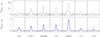 |
Fig. A.1
12CO and 13CO 1-0 spectra at the seven selected GMC positions at high-velocity resolution of 1 km s-1. The 12CO spectra of positions GMC91, GMC26 and GMC1 are taken from RPG11. The blue lines overplotted on the 12CO spectra show the Gaussian line fits used to deduce the FWHM of the lines which are listed in Table 2. |
| Open with DEXTER | |
We use the Meudon PDR code (Le Petit et al. 2006; Gonzalez Garcia et al. 2008), which solves the thermal balance, chemical network, detailed balance, and radiative transfer of a plane-parallel slab of optical extinction Av and constant density nH illuminated from both sides by an FUV field of intensity G0. The modeled line widths are calculated by the Meudon code via the Doppler broadening of the gas due to the kinetic temperature and the turbulent velocity of the gas. The latter dominates the line widths and is an input parameter to the Meudon code. We use the default value of the Meudon code which, expressed in terms of the FWHM of the velocity distribution, is (Δ v)FWHM ~ 3 km s-1. This is slightly lower than the observed line widths that are in the range of 4–11 km s-1. We also used the defaults for additional input parameters (e.g. the cosmic-ray ionization rate and size distribution of dust grains).
Initial Abundances used in the PDR models.
The grid of models has been calculated for volume densities nH = 0.1, 0.5, 1, 5, 10, 50, 102 × 104 cm-3, FUV field strengths G0 = 10, 50, 100 in Habing units, and optical extinctions Av = 2–50 mag, i.e. in steps of log Av ~ 0.2.
The input range of FUV fields is motivated by the range of FUV fields derived from the TIR in the six observed clouds which vary between G0 = 11.3 and 50.7, excluding position no2 with a very low G0 of 2.5 (cf. Table 2). We add models of G0 = 100 to cover possible higher local radiation fields. The values of AV range from those found in translucent clouds with 2 mag to extinctions of 50 mag typically found in resolved Galactic high-mass star-forming clouds. The densities cover values found in a typical molecular cloud, covering the critical densities of the observed tracers and transitions.
We calculated this grid of models for solar and subsolar metallicities. Table A.1 shows the abundances measured in M 33 and in the Orion nebula which we use as initial abundances for our PDR models. The abundances of the sun are listed for comparison. For the “solar” metallicity model, we adopt the abundances of O, C, N, S, Fe measured in the H ii region of the Orion nebula by Simón-Díaz & Stasińska (2011). The heavy elements S and Fe are depleted to dust grains with respect to the abundances found in the solar photosphere.
For the subsolar metallicity PDR model, we adopt the averaged O, N, and S abundances measured in M 33 from Magrini et al. (2010) who targeted 33 H ii regions between 1 and 8 kpc galacto-centric distance. The carbon gas-phase abundance has not been measured in M 33. We estimate it using the metallicity dependence of the C/O ratio described by (Henry et al. 2000). To derive the Fe abundance, we scale the solar Fe/O ratio by the subsolar O metallicity of M 33.
Appendix B: Chi-squared fitting and Monte Carlo analysis
To quantitatively compare the modeled and observed line ratios we calculate the summed squared residuals weighted by the observational errors between the modeled and observed line ratios HCO+/HCN and HCN/CO, for every model and for each observed cloud as 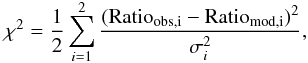 (B.1)where σ is the observational error of the line ratios deduced from the errors of the line intensities, cf. Sect. 2. We normalize the χ2 by dividing by N = 2, the number of independent observed line ratios. The minimum χ2 gives the best-fitting model.
To get a handle on the errors of the best-fitting models, we employ a Monte Carlo simulation. We assume that the measured ratios and their errors follow a Gaussian distribution with an expected value equal to the ratio and a variance equal to σ2.
We generate 5000 sets of HCN/CO and HCO+/HCN ratios drawn randomly from their Gaussian parent distribution. For every set we calculate a χ2 as explained above and deduce the best fits. From all best fits of all sets we derive the mean and the standard deviation of the input parameters: nH, Av, FUV, and χ2 (Table 5).
Appendix C: GMC properties
For comparison we derived complementary properties, the star formation rate, the FUV field, the XCO factor, the masses of the molecular and atomic material, and the optical extinction within the beam at the observed positions (Table 2). Below, we explain in detail how these values have been derived. All errors are calculated using Gaussian error propagation. The particular uncertainties of individual measurements used to derive the complementary quantities are given below.
C.1. Star formation rate (SFR) and total infrared luminosity (TIR)
To obtain an extinction free tracer of the SFR we combine the 24 μm (Tabatabaei et al. 2007) and H luminosity (Hoopes & Walterbos 2000) using (Calzetti et al. 2007). We assume errors of 7% for 24 μm (Spitzer Observers Manual v8.0) and 15% for H.
Another measure of the SFR is the total infrared luminosity (LTIR) emitted between 1 μm and 1 mm. We estimate it by adding the measured brightnesses at 24, 70, 100, 160, 250, 350, 500 μm, in W kpc-2 weighted by the factors determined by Boquien et al. (2011). We convert the determined brightnesses to luminosities corresponding to the 28′′ beam by multiplying with the beam size in kpc-2. The errors on the derived TIR are the σ values of the fits given by Boquien et al. (2011).
C.2. Molecular line luminosities
We calculate the molecular line luminosities  and
and  in units of K km s-1 pc2 by multiplying the integrated line intensities with the beam size in pc2, i.e. 1.5 × 10⁴ pc2. Errors follow from the measurement uncertainties given in Table 2.
C.3. FUV flux G0
The FUV flux G0 impinging on the dusty cloud surfaces can be estimated from the emitted total infrared intensity assuming that all FUV photons are absorbed by the dust. We use G0 = 4π 0.5 LTIR (cf. e.g. Mookerjea et al. 2011) with G0 in units of the Habing field 1.6 10-3 erg s-1 cm2 (Habing 1968) and the TIR intensity in units of erg s-1 cm-2 sr-1. Errors follow directly from the errors on LTIR. The FUV flux that we use to compare with values deduced from the stacked spectrum is the average FUV flux of all individual clouds, i.e. 21.6 ± 0.7 G0.
C.4. XCO factor and atomic and molecular gas mass
To derive the masses of the molecular gas we first convert the CO 1–0 integrated intensities into H2 column densities (NH2) via NH2 = ICOXCO. We assume that the conversion factor XCO (cf. Table 2) is a function of total infrared luminosity as found by Israel (1997) for a sample of low-metallicity environments in the LMC and SMC and for two clouds in M 33 (cf. Leroy et al. 2011).
Israel (1997) derived NH2 for CO clouds in the LMC, the SMC, and other low-metallicity galaxies from their far-infrared surface brightness and H i column densities. He finds local XCO values up to a magnitude higher than the widely used Galactic value of 2 × 10²⁰ (K km s-1)-1 cm-2 (e.g. Dame et al. 2001). In particular he studies the two bright H ii regions NGC 604 and NGC 595 in M 33, for which he derives X-factors of 22 × 1020 (K km s-1)-1 cm-2 and 12 1020 (K km s-1)-1 cm-2. Israel (1997) further finds a correlation between XCO and the TIR-flux. For NGC 604 we find a TIR luminosity of 27.18 and 7.82 × 10⁶ L⊙ for NGC 595 (cf. Sec. C.1). We estimate the local XCO for our seven clouds from their TIR by using the mean of the XCO/LTIR ratio of NGC 604 and NGC 595 as a conversion factor, i.e. XCO = 1.17 × 10²⁰ 10-6 L⊙LTIR. The derived X-factors vary between 7 and 1.5 in units of 1020 (K km s-1)-1 cm-2 for the six positions with HCN and HCO+ detections (Table 2). Gratier et al. (2010) assume a constant X-factor of 4 × 10²⁰ (K km s-1)-1 cm-2.
The mass of the molecular gas MH2 is estimated from the intensity of the 12CO 1–0 line using the XCO-factor derived in the previous section and MH2 = 2 × 1.36 NH2 mp A with the proton mass mp, the beam size A. The factor two accounts for the two protons of molecular hydrogen and 1.36 includes the contribution of heavy elements to the total mass. Errors follow from the measurement uncertainty of 12CO given in Table 2.
The mass of the atomic gas is estimated from the intensity of the H i line via the column density (Rohlfs & Wilson 2000) assuming optically thin emission. The atomic gas mass is calculated with the same formula as for the molecular mass without the factor two accounting for the two protons in H2. Errors assume a 15% calibration error on the HI data.
C.5. Optical extinction Av
As shown by Bohlin et al. (1978) a correlation between the amount of hydrogen atom column density N(H i + H2) and the color excess exists; they estimate a conversion factor of ⟨ N(H i + H2) ⟩ /E(B − V) = 5.8 × 10²¹ atoms cm-2 mag-1. The color excess and the optical extinction Av are also linked. Bohlin et al. (1978) give a value for the interstellar average of R = Av/E(B − V) = 3.1. Using the two conversion formula and the values for and NH2, derived as explained in the previous section, we calculate an estimate of the optical extinction for the observed clouds per beam. For clouds not filling the 115 pc beam, local extinctions may be higher. The errors given for Av (cf. Table 2) include the errors of N(H i) and N(H2). We estimate the Av for the stacked spectra by averaging the values of the individual positions, i.e. 4.2 ± 1.9 mag.
Appendix D: LTE column densities
LTE column densities at the individual positions.
We estimate column densities from the integrated intensities, assuming LTE and optically thin emission: 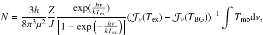 (D.1)with:
 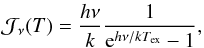 (D.2)where Z the partition function, J the rotational quantum number of the upper level, μ the dipole moment, Tex the excitation temperature, TBG the temperature of the cosmic background, and Tmb the main beam temperature of the specific line. Table D.2 lists frequency, μ, Eu/kb, and the critical densities of the observed transitions. The partition function is taken from the “Cologne Database for Molecular Spectroscopy” (CDMS) (Müller et al. 2001, 2005). The value of Z depends on Tex. The CDMS lists values for discrete temperatures in the range from 2.75 to 500 K for every molecule. We use these values to interpolate Z for the excitation temperature we adopt at a specific position.
Molecule parameters.
To estimate the excitation temperature, we derive the dust temperature, assuming that Tex, the kinetic temperature Tkin, and the dust temperature Tdust are coupled and equal. To estimate Tdust we obtain the dust SEDs for all our pointings from the Herschel and Spitzer observations at 500, 350, 250, 160, 100, and 24 μm 28′′ resolution and fit two-component graybody models to the data. Each component is described by Sν = B(ν,T)τν = B(ν,T)κνMd/D2, assuming optically thin emission, with the flux Sν, the Planck function Bν, the opacity τν, the dust mass Md, the distance D, and the dust absorption coefficient κν = 0.4(ν/(250 GHz))β cm2 g-1 (Kruegel & Siebenmorgen 1994; Krügel 2003), β is the dust emissivity index assumed to be 1.5.
Tdust is found to vary only slightly, between 20 K in the northernmost position observed, GMC no2, and 26 K in the nuclear
GMC, GMC1 (cf. Table D.1). We assume that Tex equals the temperature of the cold dust component.
The CCH 1–0 transition is split into six hyperfine components. In the stacked spectrum, we detected the 3/2–1/2, 2–1 transition, which is the strongest one. To determine LTE column densities of CCH, we estimate the total integrated intensity of the CCH 1–0 line including all hyperfine components by dividing the result of a Gaussian fit to the detected component by its relative strength, i.e. 0.416 (Padovani et al. 2009).
The column density of H2 is estimated from 13CO 1–0, assuming a 12CO/13CO abundance ratio of 60 as typically found in the Milky Way (Langer & Penzias 1993) and a H2/CO abundance ratio of 8.5 × 10⁻⁵, also found for the Milky Way (Frerking et al. 1982). From this we derive the relative abundances of the different species with respect to NH2. The derived column densities, as well as the relative abundances, are given in Table D.1 for individual clouds and in Table 3 for the stacked spectra. For comparison we give in Table D.1 the values of NH2 that we derive from the 12CO 1–0 lines using the individual XCO-factors derived for every cloud (see above). After comparing both methods to obtain the column density of H2, we find that the results are consistent within a factor of 2.5 excluding position no2. The values of NH2 for the stacked values in Table 3 are deduced using an average over the individual XCO factor of the observed GMCs of 3.0 × 10²⁰ (K km s-1)-1 cm-2.
Appendix E: PDR Model results
The modeled abundances and intensity ratios of the ground-state transition of HCN, HCO, and 12CO using the Meudon PDR code for subsolar and solar metallicities are shown in Tables E.1 and E.2. Both tables are subdivided in three blocks one for each modeled radiation field of G0 = 10,50,and 100 in Habing units, which illuminates the modeled clouds from both sides. The other two input parameters that have been varied are the density with values of nH = 0.1, 0.5, 1, 5, 10, 50, 102 × 104 cm-3 and the optical extinctions with values of Av = 2, 4, 6, 10, 16, 26, 40, and 50 mag.
Results of the PDR models with solar metallicities.
© ESO, 2012
Current usage metrics show cumulative count of Article Views (full-text article views including HTML views, PDF and ePub downloads, according to the available data) and Abstracts Views on Vision4Press platform.
Data correspond to usage on the plateform after 2015. The current usage metrics is available 48-96 hours after online publication and is updated daily on week days.
Initial download of the metrics may take a while.