| Issue |
A&A
Volume 548, December 2012
|
|
|---|---|---|
| Article Number | A29 | |
| Number of page(s) | 20 | |
| Section | Catalogs and data | |
| DOI | https://doi.org/10.1051/0004-6361/201219105 | |
| Published online | 14 November 2012 | |
The North Ecliptic Pole Wide survey of AKARI: a near- and mid-infrared source catalog⋆
1
Astronomy Program, Department of Physics and Astronomy, FPRDSeoul National
University, Kwanak-Gu, 151-742
Seoul, Republic of
Korea
e-mail: This email address is being protected from spambots. You need JavaScript enabled to view it.
2
Institute of Space and Astronautical Science, Japan Aerospace
Exploration Agency, Sagamihara, 229-8510
Kanagawa,
Japan
3
Graduate School of Science, Nagoya University,
Furo-cho, Chikusa-ku, Nagoya,
464-8602
Aichi,
Japan
4
Korea Astronomy and Space Science Institute,
305-348
Deajeon, Republic of
Korea
5
Yonsei University Observatory, Yonsei University,
120-749
Seoul, Republic of
Korea
6
RALSpace, The Rutherford Appleton Laboratory,
Chilton, Didcot, Oxfordshire
OX11 0QX,
UK
7
Astrophysics Group, Department of Physics, The Open
University, Milton
Keynes, MK7
6AA, UK
8
Academia Sinica, Institute of Astronomy and Astrophysics,
Taiwan
9
Institute for Astronomy, University of Hawaii,
2680 Woodlawn Drive,
Honolulu, HI, 96822, USA
10
Department of Particle and Astrophysical Science, Nagoya
University, Furo-cho,
Chikusa-ku, 464-8602
Nagoya,
Japan
11
The Astronomical Observatory of the Jagiellonian
University, ul. Orla
171, 30-244
Kraków,
Poland
12
Polish Academy of Sciences, al. Lotników, 32/46, 02-668
Warsaw,
Poland
13
The Andrzej Sołtan National Centre for Nuclear
Research, ul. Hoża
69, 00-681
Warsaw,
Poland
Received: 24 February 2012
Accepted: 23 July 2012
Abstract
We present a photometric catalog of infrared (IR) sources based on the North Ecliptic Pole Wide field (NEP-Wide) survey of AKARI, which is an infrared space telescope launched by Japan. The NEP-Wide survey covered 5.4 deg2 area, a nearly circular shape centered on the NEP, using nine photometric filter-bands from 2−25 μm of the Infrared Camera (IRC). Extensive efforts were made to reduce possible false objects due to cosmic ray hits, multiplexer bleeding phenomena around bright sources, and other artifacts. The number of detected sources varied depending on the filter band: with about 109 000 sources being cataloged in the near-infrared (NIR) bands at 2−5 μm, about 20 000 sources in the shorter parts of the mid-infrard (MIR) bands between 7−11 μm, and about 16 000 sources in the longer parts of the MIR band, with ~4000 sources at 24 μm. The estimated 5σ detection limits are approximately 21 mag (mag) in the 2−5 μm bands, 19.5−19 mag in the 7−11 μm, and 18.8−18.5 mag in the 15−24 μm bands in the AB magnitude scale. The completenesses for those bands were evaluated as a function of magnitude: the 50% completeness limits are about 19.8 mag at 3 μm, 18.6 mag at 9 μm, and 18 mag at 18 μm band, respectively. To construct a reliable source catalog, all of the detected sources were examined by matching them with those in other wavelength data, including optical and ground-based NIR bands. The final band-merged catalog contains about 114 800 sources detected in the IRC filter bands. The properties of the sources are presented in terms of the distributions in various color–color diagrams.
Key words: methods: data analysis / catalogs / infrared: galaxies / surveys
The full version of Table 4 is only available at the CDS via anonymous ftp to cdsarc.u-strasbg.fr (130.79.128.5) or via http://cdsarc.u-strasbg.fr/viz-bin/qcat?J/A+A/548/A29
© ESO, 2012
1. Introduction
AKARI, an infrared (IR) space telescope launched by ISAS/JAXA in 2006 (Murakami et al. 2007), successfully carried out an all-sky survey at mid- and far-IR wavelengths, as well as several large-area surveys and many other pointed observations across the wavelength range 2−160 μm. The North Ecliptic Pole (NEP) survey (Matsuhara et al. 2006) was one of these large area surveys of AKARI. The AKARI telescope had two focal-plane instruments: the Infrared Camera (IRC, Onaka et al. 2007) and the Far-Infrared Surveyor (FIS, Kawada et al. 2007). The FIS covered a 50−200 μm range with four wide-band photometric filters, and a Fourier Transform Spectrometer (FTS). The IRC was designed to carry out NIR to MIR imaging with nine photometric filters, and spectroscopic observations with a prism and grisms.
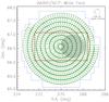 |
Fig. 1 Overall map of the NEP-Wide field. The survey consisted of 446 pointing observations represented by green boxes. Each frame covered a 10′ × 10′ area with half of its field of view (FoV) overlapped by neighboring frames. The red box and blue lines represent the regions covered by optical surveys at the CFHT and Maidanak Observatory, respectively. The circular gray-shaded region denotes the NEP-Deep field. |
The NEP survey is composed of two parts: a wide (henceforth NEP-Wide) survey and a deep (henceforth NEP-Deep) survey. The area observed in the NEP-Wide survey is shown in Fig. 1 (green tiles) and is about 5.4 deg2 with a circular shape (whose radius is about 1.25 deg) centered on the NEP (α = 18h00m00s, δ = + 66°33′38′′), while the NEP-Deep survey covers about 0.6 deg2 (Wada et al. 2008; Takagi et al. 2012), with a center slightly offset from the NEP (shaded region). These surveys were observed using the nine IRC bands to provide nearly continuous coverage from 2 μm to 25 μm. The filter system is designated as N2, N3, and N4 for the NIR bands, S7, S9W, and S11 for the shorter part of the MIR band (MIR-S), and L15, L18W, and L24 for the longer part of the MIR bands (MIR-L) with the numbers representing the approximate effective wavelengths in units of μm. The photometric bands with wider spectral widths are indicated by a W at the end. The NEP-Wide survey was carried out with 446 pointed observations, with the field of view (FoV) of each individual frame being 10′ × 10′. The survey coverage was designed around seven concentric circles and a partial rim in the outermost part.
The details of the strategy, the observational plans for the coordinated pointing surveys, the scientific goals and the technical constraints are described in Matsuhara et al. (2006). The initial results and the catalog for NEP-Deep survey were reported by Wada et al. (2008). The data characteristics and basic properties of the sources were presented using a subset of NEP-Wide data by Lee et al. (2009). Here, we present the entire data set of NEP-Wide, correct to remove artificial effects, and provide a more detailed analysis of the photometric results. The main purposes of this paper is to present the data reduction methodology, and provide a point source catalog of the NEP-Wide survey.
This paper is organized as follows. In Sect. 2, we present details of the data reduction process, and the additional image corrections needed to improve the efficacy of the image data. We describe the results of our source extraction and photometry, as well as the properties of the data such as sensitivity and the completeness of the source detection in Sect. 3. The next section describes the source matching across the available bands to confirm the genuineness of the detected sources in Sect. 4. In Sect. 5, we present the band-merging procedure and describe the contents in the final catalog. The natures of the detected sources using various color-magnitude diagrams and color–color diagrams are shown in Sect. 6. We summarize our results in the final section.
2. Data reduction
2.1. Pre-processing
2.1.1. Standard reduction with IRC pipeline
The individual pointing data from the AKARI NEP-Wide field was obtained using the observation template “IRC03” (Onaka et al. 2007), which was designed for general imaging observations. During a single pointing observation with IRC03, each exposure consisted of observations with three combined filters (two MIR bands and one NIR band). Figure 2 shows the overall view of the observation sequence, as well as the structure of the raw data obtained from a single pointing observation using “IRC03”. Each pointing data was reduced by the IRC imaging pipeline (Lorente et al. 2008) implemented in the IRAF1 environment. We adopted the official package version 0710172 without any modification of the CL script. The pipeline is composed of three stages, correcting for the instrumental features and transforming the raw data packets to basic science data as described below.
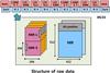 |
Fig. 2 Overall view of the observation template IRC03, which was used for NEP-Wide observations. For one pointing observation, the exposure was carried out according to a fixed sequence. The structure of the raw data obtained in the IRC03 mode are shown in the bottom panel. The NIR data consist of one short and one long-exposure, whereas the MIR data are composed of one short- and three long-exposures. |
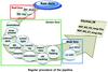 |
Fig. 3 Schematic view of the procedures in the pipeline designed for the preprocessing of the IRC imaging data. The imaging pipeline is composed of three parts. |
The conceptual structure of the pipeline is schematically shown in Fig. 3. The structure of the packaged raw data for each individual pointed observation is a three-dimensional cube that consists of combined single frames created during each exposure cycle as shown in Fig. 2. The first stage, called the “red-box” module, slices these into standard two-dimensional image frames and creates an observation log containing the summary of the processed files in the working directory. Each data set can be recognized by its target name, filter name, pointing identification number (PID), and coordinates (RA, Dec). Most of these procedures are automatically carried out by running the “prepipeline” command.
In the second stage (the green-box module), the pipeline performs various procedures such as masking of bad pixels, subtraction of dark current, linearization of detector response, and correction for distortion and flat fielding. We chose a “self-dark” parameter and the pipeline’s default flat. The self-dark is an image made by averaging pre-dark images of MIR-S and MIR-L long-exposure dark frames from each pointed observation (Lorente et al. 2008). Here, the pre-dark is the dark frame taken at the beginning of the operation for the NIR and MIR channels (Fig. 2). The super-dark was obtained from more than 100 pointings of pre-dark images taken at the early stage of the mission to provide superior signal to noise (S/N). However, self-dark may be able to remove hot pixels more efficiently than using the super-dark, especially for the MIR-S and MIR-L data. Hence, for the NIR long-exposure frames, the super-dark is used to achieve higher S/N. In the MIR data, the cosmic ray hits were removed at this stage. However, for 19 frames of the S9W and 104 frames of S11, there remained a small noticeable pattern in the lower right part even after flat-fielding. We simply removed the area having bright patterns after the pre-processing stage.
The third stage (the blue-box) calculates the relative shifts and rotations among the frames before stacking, in order to match the attitude of the frames, since the individual frames taken at a given pointing observation are not exactly aligned. In addition, the blue-box stage estimates the average sky and adjusts the sky levels before stacking these frames. We chose the default option “submedsky” for those processes. At this point, to stack the MIR-L frames, we used “coaddLusingS”. This is an optional task in the IRC pipeline, that utilizes the stacking information from the MIR-S frames, which are simultaneously obtained with MIR-L frames, thus have identical PIDs. We used this method because a successful coaddition is guaranteed thanks to the same rotations and shifts as the MIR-S frames of the same PID, even though some of them are not properly stacked when using only MIR-L images. For these tasks, we used long-exposure frames, and selected 3σ for the limits of image statistics in the pipeline reduction. Finally, the IRC pipeline adds header information that supports the world coordinate system (WCS).
2.1.2. Astrometry
To input the information of the WCS into the stacked frame, the toolkit “putwcs” of the
pipeline calculates astrometry by matching the bright point sources in the IRC image to
reference objects using the Two-Micron All-Sky Survey (2MASS) data (Skrutskie et al.
2006). The astrometric accuracy of the “putwcs”
is less than 1′′ rms for the NIR bands, about 2′′ rms for MIR-S bands, and 3′′–4′′ rms
for MIR-L bands (Wada et al. 2008; Shim et al.
2011). The full-width-at-half-maximum (FWHM) of
stacked frames from a pointing observation are about
 in the NIR bands, and in the range
 –
– in the MIR bands (Lorente et al. 2008; Lee et al. 2009) depending on the filter.
The “putwcs” was run automatically from the N2 to S9W band images. However, this task did not work well for the wavelength bands longer than S9W because of an insufficient number of sources with 2MASS counterparts. For this reason, the astrometry for about 40 frames (~9%) of the S11 band was derived by comparing with the S9W frames whose WCS solutions had already been determined. This alternative method was satisfactory because the S11 frames with unsuccessful “putwcs” operations constituted only a small fraction of the total, and the sources in these S11 frames were easily identified using S9W data with the same PID. At this stage, three sets of pointing data from the NIR bands were discarded owing to stacking failures and very low quality (PID: 2110888). For the L15 band, the automatic operation of “putwcs” was successful for only 84% frames. The astrometry of the remaining ~16% was done using S11 sources in the same manner as described above for S11 frames. However, the pointing direction of the MIR-L channels is ~20.6′ apart from that of the MIR-S, while the NIR and the MIR-S share the same field of view. Therefore, to utilize S11 sources for the astrometry of the L15 data, we used pertinent regions extracted from the mosaicked image of the S11 band.
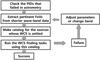 |
Fig. 4 Schematic flow chart describing the iterative procedures used to find a satisfactory solution for the WCS header of the L18W and L24 band data. |
The astrometric solutions for the L18W data were obtained in a similar way to that for the L15 band. However, the number of common sources between the L18W band and 2MASS data was quite small so that the “putwcs” operations were applicable to only about 50% of the L18W frames. The remaining frames were processed using the L15 sources, but these attempts were also not fully successful because, for many frames, the number of L18W sources cross-matched with L15 sources was insufficient. For these frames, we used the corresponding region extracted from the mosaicked images of the S11 and S9W bands. For the L24 band, the automatic execution of “putwcs” was able to find the astrometric solution for only ~10% frames of the total since 24 μm sources with 2MASS counterparts are very rare. We therefore conducted an alternative source-matching with the L18W and L15 band data and obtained the astrometry for about 65% of the frames. To get correct astrometry using WCS deriving tasks, we have to ensure a sufficient number of sources effectively available for the fitting process of the software. The iterative procedures adopted to find a sufficient number of sources for the astrometry of the L18W and L24 data are shown schematically in Fig. 4. We were able to obtain astrometric solutions for about 90% of the L24 frames, leaving ~10% of the frames unusable for source detection and photometry.
2.2. Post-processing and image correction
2.2.1. Cosmic ray rejection in the NIR bands
The “IRC03” template takes three long-exposure frames for each NIR band. The last frame N4 in each pointed observation may be taken during a satellite maneuver to the next pointing, and can be automatically rejected by the pipeline when the data quality is too poor (Fig. 2). For this reason, most of the N4 pointing data have two frames stacked by the pipeline. This causes difficulties in removing cosmic rays from N4 frames (as well as a small fraction of the N2 and N3 frames). Therefore, an alternative method to remove cosmic rays from individual frames has to be applied to those frames before the mosaicking. We used a program “L.A. cosmic” which is based on the Laplacian edge detection algorithm for highlighting boundaries (van Dokkum 2001). We used the imaging version3 of the software written in CL script for IRAF users provided by van Dokkum4. This procedure relies on the sharpness of the edges rather than the contrast between entire cosmic rays and their surroundings, therefore it is independent of their shapes. The L.A. cosmic procedure was run by the implementation in IRAF with the default settings. This algorithm was found to be quite robust and it effectively rejected remaining cosmic rays of arbitrary size.
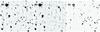 |
Fig. 5 Example showing the result of cosmic-ray rejection. The left panel a) is a sample portion of the N4 image produced by the IRC imaging pipeline (PID: 2100757) on which many cosmic rays remain. The middle panel b) is the same image restored by cosmic-ray rejection using the L.A. cosmic procedure. The third panel c) shows the result of subtraction, a–b, which is just a map showing the rejected cosmic rays. |
Figure 5 shows an example comparison of the images before (left panel) and after the procedure (middle panel). The right panel shows the difference between the two images. However, the sources directly hit by cosmic rays are consequently deformed or damaged during the L.A. cosmic procedure, hence the photometry for those sources are inevitably affected. Most of these sources damaged by cosmic rays were finally rejected by the masking process during the image correction to remove MUX-bleeding effects in the NIR bands, as described in the following section.
2.2.2. Correction for MUX-bleeding effects
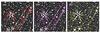 |
Fig. 6 Close-up views of a sample region around bright sources showing false detections at each NIR band caused by MUX-bleeding trails before the correction. The left, middle, and right panels show the N2, N3, and N4 band images, respectively. Colored circles indicate the objects that were not matched with optical data. |
In addition to cosmic rays, multiplexer bleed trails (or MUXbleeds, hereafter) remained along the horizontal direction in the NIR data because of the nature of InSb detector array (Holloway 1986; Offenberg 2001). In general, when there is a bright source in a frame, periodic horizontal features appear along the same row. Consequently, many spurious artifacts are detected as sources along the bleeding trails. Figure 6 shows the region where the spurious detection is serious due to MUXbleeds. To mitigate such artifacts, and facilitate detection and accurate positional matching with real source in the other bands, we have to apply an appropriate rejection procedure. However, it is difficult to accurately correct for the bleeding effect without any influence on the real sources. We simply masked the regions of MUXbleeds, at the expense of rejecting a small number of real sources.
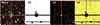 |
Fig. 7 Schematic diagram describing the procedures used to make a weight map for an individual frame obtained from a single pointing observation. The first panel a) is a sample image containing a bleeding trail and a bright source whose center is disrupted. The second panel b) shows the regions to be masked. The third panel c) represents the number of rejected frames during the stacking procedure. Each pixel has an integer value ranging 0 to 3. The last panel d) is a weight map to be used for the final mosaicking procedure. |
The method we used to mask the region severely affected by bleeding effects assigns a different weight to the selected regions when we create a mosaic image with the software SWarp5. When we wished to remove a region affected by MUXbleeds we gave a zero weight to that region. Figure 7 shows a schematic overview describing the steps adopted to determine the region to be masked and to produce a weight map, which is used to generate a mosaic image at the final stage. The leftmost panel (a) is a sample image reduced by the IRC pipeline. In the second panel (b), dark stripes and circles show the regions to be masked by assigning a zero weight, whereas the white regions have 100% weight. The third image (c) shows the number of rejected frames during the stacking procedure in the final stage of the pipeline. For example, there are three dithered exposures in the N2 band and each pixel in this map may have an integer value ranging from 0 to 3. If we multiply this by “mask image” of the second panel, we can make the final weight map in the panel (d), which gives proper weight factors for individual pixels. Here, the most important task is how to decide the region to be masked to effectively remove the muxbleeds while minimizing the pixel losses that were not affected by the bleeding trail.
To decide the area to be masked, we had to trace the bright sources causing MUXbleeds. We investigated the threshold brightness at which MUXbleeds started to appear. We carried out photometry on all of the individual frames to find the sources brighter than this threshold. The photometry was done both before and after the L.A. cosmic procedure to search for the sources hit by cosmic rays and deformed during the cosmic ray rejection process. The results of these measurements enabled us to determine the area to be masked, as well as the sources distorted by cosmic rays. The typical shape of the masked region around a bright source is a circular disk centered on the centroid of the source, with a narrower horizontal stripe covering the bleeding trail. We found that sources brighter than ~12.6 mag (mag) cause MUXbleeds in the N2 band, and sources brighter than about 13 mag in the N3 and N4 bands. The radius of the circular area and the width of the stripe both depend on the brightness of the source. For the circular mask, the center is defined by the pixel coordinate of the source that causes the bleeds, and the appropriate radius was chosen to be 2.5 times of the Kron radius (Kron 1980). The width of the stripe was set to be 1.5 Kron radius, and the actual position of stripe was 2–3 pixels parallel-shifted in a vertical direction from the original y-coordinate of the source to efficiently block the MUXbleed, because it is not symmetric with respect to horizontal axis. Applying these criteria on each frame, we masked the MUXbleeds and extremely bright sources (brighter than 12.6 mag) as well as the sources deformed by the cosmic ray rejection procedure in the NIR bands.
In the MIR bands, the MUXbleeds have less significant effects on the image frames because the bleeding trails are rarely found in the S7 and S9W bands, and completely disappear in the S11 band. Since the horizontal trails usually do not extend to the edge of frame, we used small patches covering the trails around the source in order not to lose too many pixels. However, in 19 frames in the S9W and 104 frames in the S11 bands, a bright bean-shaped pattern remained in the corner of the frames. Artifacts occasionally caused by moving objects such as satellites or asteroids passing through the field of view were also found in four frames in the MIR-S bands. To reject these bright artifacts, masking regions were carefully determined by visually inspecting the individual frames and weight maps were generated that were used for image mosaicking basically in the same manner as the NIR data. The number of frames that require weight maps for mosaicking was about 10% of the MIR-S data.
2.2.3. Weight maps and mosaic images
To create a mosaic image for each band, we combined individual frames using SWarp. During the SWarp run, the “WEIGHTED” option was selected as a combine type in order to use the weight maps generated for MUXbleed correction. The BILINEAR resampling method was also used since it is known to be effective at suppressing boundary discontinuities. In the final mosaic images, spiky structures still remained close to bright sources because they are difficult to remove unless we apply rather large circular radii when masking these regions. However, these structures do not occupy a significant fraction and do not cause serious false detection problems. False sources are easily filtered out during the confirmation procedure that uses data from other bands (see Sect. 4).
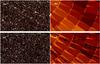 |
Fig. 8 Segments of mosaic images (left) and weighted coverage maps (right) before and after the MUXbleed correction (N3). The upper pair shows the images before this process and the bottom panels show them after the operation. The bleeding trails in this field are completely removed by this weighted mosaicking method using weight maps. In the map d), zero-weighted pixels are in black. |
Figure 8 shows the results of the image correction for MUXbleed effects using two pairs of maps. The upper panels are mosaic (left) and weight (right) maps before correction, whereas the bottom panels show the corresponding images after correction. Most of the bleeding trails in the NIR bands are effectively removed by this process. By co-adding the individual pointed observations, utilizing the weight map for each frame, we finally produced three NIR master images for the source extraction and photometry. Among 446 frames, three were excluded owing to the stacking failure in the pipeline caused by the poor data quality. The actual area covered by the NIR bands is about 5.34 deg2 and the fraction of masked region is in the range of 2–4% of the observed area. As summarized in Table 1, about 0.21 deg2 was masked out in the N2 band, which is about 4% of the entire area covered by the N2 band. In the N3 band, 0.198 deg2 (3.7%) and in the N4 band, 0.111 deg2 (2.1%) were masked, respectively.
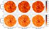 |
Fig. 9 Entire coverage maps of the NIR data before (upper) and after (lower) the correction for MUX bleeds. Uncovered area and none-weighted pixels have zero values (white area), which have wedge-like shape from the center to radially outer direction. |
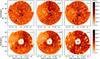 |
Fig. 10 Entire coverage maps of MIR-S (upper) and MIR-L (lower) bands. |
The weighted coverage maps may help us to understand the overall view of the final results compared to the uncorrected image data, as shown in Fig. 9. The maps for the NIR data before and after the correction are presented for comparison. The actual coverage as well as the masked area were calculated using these maps. The mosaic images for the MIR bands were generated in the same way using weight maps for individual frames, and have similar coverage maps as shown in Fig. 10.
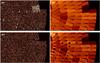 |
Fig. 11 Segments of a mosaic images (left) and weighted coverage maps (right) before and after the correction for undesirable patterns in the S9W image. The upper panels show the images before the masking and the bottom panels show the resultant images after masking. Coverage maps show that the masking of MIR-S images effectively removes most of the remaining patterns (for 19 frames), and demonstrates that remaining MUXbleed effects are almost completely removed. |
Coverage and masked area.
The areas observed by the MIR-S bands range between 5.33 and 5.35 deg2. The fraction of the masked region (zero-weighted regions) is less than ~0.03%, a very small fraction compared to those of the NIR bands (Table 1). The masking of the S7 band was mainly required because of the streaks caused by bright stars in ~25 frames. For the S9W and S11 bands, the masking was done to reject the noticeable patterns in about 19 and 104 frames in the S9W and S11 bands. Figure 11 shows the segments of resultant mosaic images of the S9W band. The upper and lower panels show the images before and after the correction for the irregular artifacts, respectively. For the MIR-L bands, this procedure was not necessary because there were no artifacts. Note that there is uncovered region near the central parts of the MIR-L observation because of the offset between the FoVs for the MIR-S and MIR-L observations (see Murakami et al. 2007, for the focal plane allocation of the instruments of AKARI).
3. Photometry and data properties
3.1. Source detection and photometry
As shown in Figs. 8 and 11, we removed most of the MUXbleed effects in the NIR bands, as well as other artifacts in the MIR bands, to minimize spurious detections. We confirmed that the detection reliability was significantly improved by comparing the detected sources from a small portion of both the corrected and the uncorrected images, using the same detection parameters.
We used the entire mosaicked images covering the whole NEP-Wide area to carry out extraction and photometry of the sources for each band. To measure the fluxes of the detected sources, we used a software SExtractor developed by Bertin & Arnouts (1996)6. Here, we chose DETECT_THRESH = 3, DETECT_MINAREA = 5, and BACK_SIZE = 3, which are the same as those used by Wada et al. (2008), except for DETECT_THRESH. We chose a higher threshold to reduce false detections. The number of detected sources from nine master images are presented in Table 2, together with the estimated detection limits as described in the following section. About 87 800, 104 000, and 96 000 sources are detected in the N2, N3, and N4 band, respectively. The numbers of detected sources in the MIR bands are much smaller than those in the NIR bands. In the MIR-S bands, 15 300 (S7), 18 700 (S9W), and 15 600 (S11) sources were detected, and in the MIR-L bands, 13 100 (L15), 15 100, (L18W), and about 4000 (L24) sources were detected, respectively.
The photometric measurements were made in a single mode operation for each band in order not to use the same aperture for different band images. The sizes of the sources depend significantly on the effective wavelengths of the filter bands because the IRC images are nearly diffraction limited. To confirm the validity of detected sources and reject spurious objects, it is more appropriate to employ the single mode operation for each band and look for counterparts in the other bands.
To use flexible apertures for various sources, the fluxes of them were measured using elliptical Kron apertures (i.e., SExtractor’s Flux_AUTO), owing to the elongated shapes of the point spread functions (PSFs) in the NIR bands as well as for the variable sizes and shapes of MIR band sources. The fluxes in units of ADU are converted to μJy using the flux calibration in Table 4.6.7 of the IRC data user manual version 1.4 (Lorente et al. 2008; Tanabe et al. 2008), which has been established based on the observation of standard stars. Finally, we obtained the AB magnitude (Oke & Gunn 1983) using the relation, AB (mag) = −2.5 log fν + 23.9, where fν is the flux density within a given passband in units of μJy.
Number of detected sources and 5σ detection limits.
We checked the reliability of the photometry by comparing our magnitudes of the bright (<16 mag) sources with those in the NEP-Deep catalog of Wada et al. (2008; see also Takagi et al. 2012). We found that the average magnitudes of the same sources in the NEP-Wide and NEP-Deep differ by up to 0.05 mag. Since the rms of magnitude differences between the NEP-Deep and Wide data were about 0.1, the systematic difference of 0.05 mag is not considered to be statistically significant. Furthermore, these differences are within the absolute calibration uncertainties (~6%). Since the observations for the NEP-Wide and NEP-Deep surveys were done with different observing templates (i.e. IRC03 for NEP-Wide and IRC05 for NEP-Deep) and the photometry was performed with slightly different parameters, we regard that the small systematic differences between the measured magnitudes are not serious.
3.2. Detection limits and completeness
The flux limit of the point source detection in each band was estimated from the fluctuation in the sky background, by measuring the flux at random positions far away from the source positions. We used an aperture three times the size of the FWHM, and determined the 5σ detection limits based on the value of σ derived from the sky background. The detection limits depend on the noise levels of the fields, which vary from place to place, and we present the averaged values over the entire NEP field in Table 2. In this table, we listed the FWHMs of sources detected in mosaicked images for all the IRC bands. For each band, we measured the FWHM for about 30 bright sources whose optical counterparts have stellarities greater than 0.95 and took the average of them. In the NIR bands, the N2 filter reaches a depth of ~20.9 mag, and the N3 and N4 bands reach ~21.1 mag. The MIR detection limits are much shallower: ~19.5 (S7), 19.3 (S9W), and 18.9 mag (S11) for the MIR-S bands, and ~18.5 (L15), 18.6 (L18W), and 17.8 mag (L24) for the MIR-L bands. In the table, the 50% completeness limits, which were measured by injecting artificial sources as described below, are also presented.
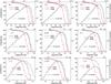 |
Fig. 12 Completeness estimation for each band (red curves). The estimates for the NEP-Deep data are also shown for comparison. The gray histograms show the NEP-Wide source density per square degree per 0.2 mag bin at each band (not corrected for incompleteness). |
Using the IRAF tasks in noao.artdata package, we generated artificial sources with a fixed range of magnitude and spread them at random positions in 8 sample regions of 10′ × 10′ selected from all over the mapped area. The sources injected at positions within a distance of 20 pixels from any other sources are not counted as input sources to avoid source blending and miscounting. We attempted to detect the injected objects and measured the brightness of them by running SExtractor with the same parameters as those applied to the detection and photometry for the real sources. We compared the positions and magnitudes of the detected sources with those of the artificial input sources. If a detected source lay within 2 pixels (1 pixel corresponds to 1.46′′, 2.34′′ and 2.45′′ for NIR, MIR-S, and MIR-L bands, respectively) from the location of the input source, and the measured brightness was within 0.5 mag of the input value, we regarded this source as valid detection of the injected source. These criteria for the validation of the detected sources are the same as those chosen by Wada et al. (2008). We then counted the number of detected sources and compared them with the number of the input artificial sources to determine the completeness, which was defined as the fraction of recovered objects in each magnitude bin. To ensure statistical efficacy, we generated a sufficient number of input sources (300–400) per sample region. For each magnitude bin, we repeated the same procedures seven to ten times with different seed numbers for the brightness and spatial distributions, and took the average. Among the various input parameters for this test, the most sensitive was found to be the half intensity radius at each wave band.
The completeness of detection for the NEP-Wide data are shown in Fig. 12 as a function of magnitude for the IRC bands. We also show the completeness estimates for the NEP-Deep data using the same parameters as those employed for the NEP-Wide data. The completeness curve shows that the detection probability begins to drop rapidly at around the 85–80% value in the NIR bands, and around the 90% level in the MIR bands. The magnitude difference between the 90% and 10% completeness is about 1 mag in the NIR bands, and less than 1 mag in the MIR bands. The 50% completeness limits are about 19.8 mag in the NIR bands, 18.7−18.3 mag in the MIR-S bands, and 18.0−16.8 mag in the MIR-L bands, as presented in Table 2. As shown in Fig. 12, the magnitude differences between the NEP-Wide and NEP-Deep data at the 50% completeness level are about 0.5−0.6 mag in the NIR and MIR-S bands. In the MIR-L bands, the differences are about 1.0 (L15)−0.5 mag (L18W).
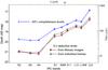 |
Fig. 13 Flux detection limits and 50% completeness limits for each band. The detection limits of the NIR bands are around 21 mag, and MIR bands reach much shallower depth than NIR bands. The 50% completeness limits are about 1.2 mag shallower than the detection limits in the NIR filters and about 0.7 mag shallower in the MIR bands from S7 to L18W. |
Figure 13 shows the comparison of the 5σ detection and 50% completeness limits for the IRC bands. The measurements of the detection limits using individual frames are also shown for comparison (gray). These estimates obtained using the mosaicked images give slightly shallower detection limits than those measured using the individual frames for the NIR band, while deeper limits are measured for the MIR bands. The differences at the NIR bands are less than 0.2 mag and possibly result from the variation of the image quality, for example from FWHM changes and seeing variations, along with resampling during the mosaicking process.
The 50% completeness limits are shallower than the 5σ detection limits by about 1.2−1.3 mag for the NIR bands and about 0.6−0.8 mag for the MIR bands (except for L24 which has a relatively larger difference of 1.0 mag). Wada et al. (2007) also found a similar trend in the differences between the 5σ detection limits and 50% completeness limits for the NEP-Deep data. By comparing a single exposure and stacked image of ten exposures, they found that the 50% limits do not improve much for the NIR bands, while the improvements for the MIR bands are close to the square-root of the exposure time. On the basis of these results, they concluded that the NIR bands are affected by the source confusion. In fact, the improvement in the 50% limit between one pointing and ten pointing observations is only a factor of 1.15 (Wada et al. 2007) for the N3 band, implying that the source confusion could be significant.
The MIR bands are unlikely to be affected by the confusion because the source density is much lower than that of the NIR bands, while the sizes of the PSFs are nearly the same (Lee et al. 2009). The smaller difference between the 50% completeness and 5σ detection limit can thus be understood by the confusion effects in the NIR bands. Note that the numbers of source per beam are 1/60.7, 1/46.8, and 1/51.3 for N2, N3 and N4 bands, respectively. These values are smaller than the classical definition of the confusion limit of 1/30 sources per beam, but only by a factor of two. The NIR band observations are affected by the source confusion to some extent.
4. Confirmation of the sources
4.1. Supplementary data
In addition to our AKARI/NEP-Wide data, high-quality optical data, NIR J and H band data, and radio data over a more limited field are available for the NEP-Wide field (Kollgaard et al. 1994; Lacy et al. 1995; Sedgwick et al. 2009; White et al. 2010). Optical data were obtained using the 3.5 m Canada-France-Hawaii Telescope (CFHT) for the inner parts and the 1.5 m telescope at Maidanak observatory in Uzbekistan for the outer parts of the NEP-Wide field as shown Fig. 1. The CFHT observations with the MegaCam covered the inner part of the 2 deg2 rectangular field centered on the NEP using the u∗, g′, r′, i′, z′ filter system. The detection limits (4σ) are about 26 mag for u∗, g′, r′, about 25 mag for i′, and 24 mag for z′ band, and the full catalog contains over ~110 000 sources (Hwang et al. 2007). The Maidanak observations were carried out using the SNUCAM (Im et al. 2010). The observations covered the outer regions surrounding the CFHT field using B, R, I filters (Jeon et al. 2010), whose depths are around 23 mag in B, R and about 22 mag in I band. In addition, NIR J, H band data was obtained using FLAMINGOS mounted the Kitt Peak National Observatory (KPNO) 2.1 m telescope, which cover the entire NEP-Wide area (~5.2 deg2). The number of sources in this data is over 220 000 (Jeon et al., in prep.). The optical data are crucial for identifying the nature of the corresponding AKARI sources, since the stellarity parameters help us to distinguish between stars and galaxies. The J, H data are used to bridge the gap in wavelength coverage between the AKARI/NIR and the optical data.
4.2. Overview of the source matching
To construct a reliable source catalog, we have to validate the detected sources. If a certain source is detected at only one filter band without any counterpart in the other bands, it could potentially be as a false detection, especially in the case of the NIR bands. In order to verify the reliability of detected sources in a given IRC band, we searched for their counterparts within a 3′′ radius in the other IRC bands, as well as ancillary optical and J, H band data search parameter. The choice of 3′′ as a matching radius is somewhat arbitrary: we considered the astrometric accuracy of the NEP-Wide data to be 1.38′′ (Lee et al. 2009), hence selected a search radius of twice of this value. We tried several values and found that the number of matched sources begins to increase very slowly with radius larger than 2′′, and nearly saturates at around 3′′. Note that the typical size of the FWHM of the point sources ranges from 5′′ (NIR) to 7′′ (MIR) (see Table 2), approximately corresponding to the diameter of the matching circle.
Number of sources matched with those in other bands.
In the case of the N2 band, for example, we first examined its positional matching with the N3 and N4 band. We then proceeded to find counterparts in the optical, and the KPNO’s J and H bands. We finally looked for the matching sources in the AKARI’s MIR-S and MIR-L data. About 1590 of the N2 sources (~1.8%) do not have any counterpart in any of the other bands. In the N3 and N4 bands, about 3.9% and 6.8% of the sources remained unmatched to any other band data, respectively. All of these unmatched sources can not be confirmed and are likely to be false objects. We excluded these sources from the catalog.
To find the counterparts of the MIR sources, a similar procedure was applied. The cross-matching of the sources in each of the MIR band was carried out against the others from the NIR to MIR-L bands in order of wavelength. The fractions of sources without any counterparts are 1.6%, 1.0%, and 2.2% for the S7, S9W, and S11, respectively. For the MIR-L bands, about 7%, 10%, and 20% of sources in the L15, L18W, and L24 bands remained unmatched to those in other bands. Unlike the NIR bands, it is risky to exclude all of the MIR sources having no counterparts because the artifacts are not serious in the MIR bands compared to the NIR bands, and very red objects can be detected in the long wavelength bands only. We therefore checked all the unmatched sources by eye and included most of them except for some very rare cases (~2%) with spurious images.
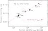 |
Fig. 14 Probability of random matching for the N2 band sources with those in other bands. The random matching probability is proportional to the density of the sources in the band to be matched, as indicated by the dotted line. |
The results of the matching procedures among the IRC bands as well as with optical data
are presented in Table 3. The numbers in this table
include the sources that were matched more than once, which are given in the parenthesis.
Duplicate sources, or multiple matching occurred predominantly when the sources were
located in a crowded region, although numerically they represent a small fraction of the
total. When two band data are used to find a counterpart, there is always a possibility of
false matching. Suppose that the sources in bands A and
B are uncorrelated and randomly distributed in space. In this case, the
fraction of the sources in band A accidentally matched with those in band
B is simply  , where rmatch
is a matching radius. We confirmed this simple relationship between the source density and
the false matching rate by numerical simulations: we tried to match the
N2 sources to those in other band data but in different fields of the
same size, the results of which are shown with diamonds in Fig. 14. A dotted line in this figure is an expected relation from the
numerical simulation. The matching experiments with the real data for random fields of
view show good agreements with the expected relation based on a random-matching
probability argument. In our cross identification procedure, the density of the optical
data is the highest: the CFHT catalog (Hwang et al. 2007) contains about 118 200 sources in 1.8 deg2 and thus the source
density is 65 700 per deg2. When we used the matching radius of 3′′, the false
matching rate was about 14.3%. For the Maidanak data, the source density is about
41 100 per deg2 and the false matching rate is estimated to be 9%.
, where rmatch
is a matching radius. We confirmed this simple relationship between the source density and
the false matching rate by numerical simulations: we tried to match the
N2 sources to those in other band data but in different fields of the
same size, the results of which are shown with diamonds in Fig. 14. A dotted line in this figure is an expected relation from the
numerical simulation. The matching experiments with the real data for random fields of
view show good agreements with the expected relation based on a random-matching
probability argument. In our cross identification procedure, the density of the optical
data is the highest: the CFHT catalog (Hwang et al. 2007) contains about 118 200 sources in 1.8 deg2 and thus the source
density is 65 700 per deg2. When we used the matching radius of 3′′, the false
matching rate was about 14.3%. For the Maidanak data, the source density is about
41 100 per deg2 and the false matching rate is estimated to be 9%.
However, these probabilities should be regarded as upper limits for the false matching since the sources detected in the same field of view should be actually correlated, i.e., a source at a given band is likely to be present in the other bands. In order to make more realistic estimates of the false matching rate, we varied the matching radius. In the case of the matching test between the N2 and CFHT optical data, for example, we found that the number of the N2 sources that have the optical counterparts in an annulus corresponding to matching radii of between 2.5′′ and 3′′ comprises about 1.41% instead of the random matching probability of 4.37%. In the case of the matching with the Maidanak data, we expect a 2.75% false matching rate for the same annulus, but only 1.08% matched sources were found. If we assumed that all the sources in this annulus had been accidently matched, the false matching could be less than 1.5%. We thus conclude that the false matching probability must be very low.
4.3. Summary of the source matching
4.3.1. Matching between IRC bands
The results of the source matching amongst the different wavebands were used to confirm the source detections. In the AKARI/NEP-Wide data, the numbers of sources in the NIR bands are much larger than those of the MIR band sources. Consequently, the majority of the MIR sources have the NIR counterparts, but not vice versa. It is therefore reasonable to combine the information on the basis of the NIR framework.
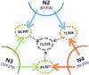 |
Fig. 15 Summary of the source matching between the different NIR bands. The numbers of sources detected in each NIR band are presented at the apexes of the triangle. The matching results amongst them are shown, excluding any duplicated or multiply matched sources. The numbers in the dotted ellipses represent the number of sources with detections in both of the matching bands. |
As explained in the previous section, a matching between any two bands was performed in both directions. Between the N2 and N3 bands, for example, we first searched for counterparts in the N3 band for a given N2 source, and then changed the matching direction. Similar procedures were applied to all the possible combinations of the three NIR bands, as shown in Fig. 15. The numbers shown in the ellipses on the three sides of the triangle are those of the number of sources, with the detections in both bands indicated at the apexes. Using the results of the cross-matching in both directions, we can find either duplicate or multiply matched sources between two bands. The number of the sources detected in both the N2 and N3 was 80 990, in the N2 and N4 was 71 898, and in the N3 and N4 was 84 807.
For a given MIR source, there could be multiple NIR or optical sources since the PSF of the MIR data is much larger than that in the NIR and the source density in the NIR is much higher (by up to a factor of eight) than that in the MIR. In such cases, we simply chose the nearest detection to the MIR source. On the other hand, there were no multiple matching of the MIR sources for a given NIR source. We summarize the results of cross matching between the NIR and MIR bands in Fig. 16. Amongst the MIR bands, there were no duplicate matches, as presented in Table 3, since the number density of the MIR sources is much lower.
4.3.2. Optical identification
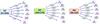 |
Fig. 16 Schematic diagram showing the results of the matching between the sources in the NIR and MIR bands except for multiply matched sources. The matching results of the N2 sources with all the MIR bands are shown in the leftmost panel. The results for N3 and N4 bands are shown in the middle and the right panels, respectively. |
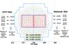 |
Fig. 17 Results of the matching AKARI sources with the optical data covering two separate fields of the CFHT and Maidanak observations. On the left and right of the diagram, the results for the CFHT and Maidanak data are presented, respectively. Overall results of the matching both sets of optical data are given in the bottom of the figure. |
On the left and right hand sides of Fig. 17, the numbers of sources matched with each of the optical catalogs are presented. Note that the total number of N3 sources is 104 170, while the number of them in the CHFT field is about 36 380. Amongst these sources, 82.8% in the CFHT field have optical counterparts. Similarly, the number of N3 sources located in the Maidanak field is about 82 750, which is more than twice the number of sources in the CFHT field, and 62.4% of these sources have Maidanak optical counterparts. On the whole, 74.1% of the N3 sources have counterparts in either the Maidanak or CFHT data. As shown in the lower part of Fig. 17, 83.0% of the N2 and 70.4% of the N4 sources have optical counterparts. The rate of matching with optical data decreases with NIR band wavelength. The matching rate with the CFHT data is somewhat higher than with the Maidanak data, because the CFHT observations are deeper.
We also examined the matching of the NIR sources with the KPNO J, H data. The cross matching results are presented in Fig. 18. For the N2, N3 and N4 bands, 78%, 63% and 65% have counterparts in KPNO data, respectively.
5. Catalog
5.1. Band-merging
After the source matching described above, we generated separate catalogs for the nine IRC bands. At this point, each catalog contained the photometric information from the other bands. We merged those catalogs step by step. As shown in Fig. 19, we made an NIR band catalog from the N2, N3, and N4 single-band catalogs by cross-matching the sources, and where possible, with the optical data. The MIR-S and MIR-L catalogs were also generated with the same method as used for the NIR catalog. The final band-merging was based on the NIR catalog, and the sources in the MIR-S and MIR-L catalogs were compiled by matching of the entries using corresponding source IDs. For registered sources in the catalog, if there was no detection in a certain band, we assigned the dummy value 99 000. The NIR sources having no counterpart in any other bands are excluded to avoid the false objects caused by various artifacts. As explained in Sect. 4.2, however, we carried out a careful eye inspection of the individual images of the MIR sources with no counterparts before this exclusion.
5.2. Catalog format
The number of sources in the final catalog is about 114 800. In Table 4, an extract from the source catalog is shown for the purpose of illustration. We give a short description below of the columns in the catalog.
Column (1) contains the identification number of the sources.
-
Columns (2) and (3) are the J2000 right ascension (RA) and thedeclination of a source in decimal degrees. The coordinates arebased on the N2 astrometry. If there was no detection in the N2 image, thecoordinates were based on the shortest wavelengthidentification.
-
Columns (4), (7), (10), (13), (16), (19), (22), (25), and (28) are the AB magnitudes of the sources in the AKARI bands from the N2 to L24 band.
-
Columns (5), (8), (11), (14), (17), (20), (23), (26), and (29) provide the uncertainties in the magnitudes, which are the RMS errors in the measured values.
-
Columns (6), (9), (12), (15), (18), (21), (24), (27), and (30) are the photometric flags from the SExtractor. 0 – well isolated and clean image, 1 – the source has neighbors, about 10% of the integrated area affected, 2 – the object was blended with another one, 3 – 1 + 2, 4 – at least one pixel is saturated, 8 – object is truncated, close to the image boundary, –1 – no photometry (not detected).
-
Column (31) is the additional flag that indicates any caution about the use of the NIR photometry, (this indicates partially damaged sources during the cosmic-ray rejection, masking of MUX-bleeding, and etc.) 2 – for N2, 3 – for N3, 4 – for N4. For the matching results with optical data, we present the magnitude, magnitude error, and stellarity information. In addition, the number of matched optical sources and the positional deviation of optical source from the AKARI WCS are included.
-
Columns (32), (34), (36), (38), (40) are the magnitudes in u∗, g′, r′, i′, z′ from the CFHT data.
-
Columns (33), (35), (37), (39), (41) are the magnitude errors in u∗, g′, r′, i′, z′.
-
Columns (42), (44), (46) are the magnitudes in B, R, I from Maidanak data.
-
Columns (43), (45), (47) are the magnitude errors in B, R, I.
-
Column (48) contains stellarity information from optical data. Note that the stellarity values for the CFHT data were measured from the g′, r′, i′, z′ combined image (Hwang et al. 2007) and those of the Maidanak data were determined from the R- band image because of its highest S/N (Jeon et al. 2010). If a source is matched with both the CFHT and Maidanak data, we used the stellarity determined from the CFHT data.
-
Column (49) provides the number of optical sources matched to an AKARI source. For multiply matched sources, this is larger than 1.
-
Column (50) contains the distance between the astrometric coordinates of AKARI and optical data in arcsec. When an AKARI source is matched to optical data more than once (that is, Col. (49) > 1), we chose the smallest number (the value of the closest one).
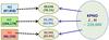 |
Fig. 18 Number of sources in each of the NIR band detection catalogs matched with KPNO J, H band data. About 78%, 63%, and 65% of the N2, N3, and N4 sources were found to have counterparts in the J and H band data. |
6. Nature of the sources
The point sources in the NEP-Wide catalog are mostly either stars or galaxies. In high-resolution optical images, the galaxies appear as extended sources unless they are very far away or very compact, whereas stars appear as point sources whose images follow the PSF of the instruments. However, in the AKARI image, distant galaxies cannot be easily distinguished from those of stars because of the relatively large PSFs. In many cases, the nature of the sources can be identified by their spectral energy distributions (SEDs).
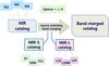 |
Fig. 19 Schematic diagram describing the band merging procedure. we first combined the three catalogs of the NIR, MIR-S, and MIR-L channels. We then merged them into a band-merged catalog covering the optical u∗ to the L24 band. During this procedure, we checked the source IDs carefully in order to avoid any duplication of the same entries. |
In contrast to the infrared images, the ground-based optical images have much smaller PSFs, allowing an easy distinction between the point and extended sources. In particular, the optical data for the NEP-Wide were all taken in excellent seeing conditions. Both the CFHT and Maidanak data have typical PSF FWHMs smaller than one arcsecond. The stellarity parameter given by SExtractor can thus be used to distinguish between point and extended sources, as shown in Fig. 20. The sources with stellarity parameters close to 1 are point-like sources, while those with values close to 0 are extended sources. Although the stellarity parameters are spread over all the possible values between 0 and 1, there is a clear dichotomy, unless the sources become too faint. For the following discussion, we selected the high-stellarity sources using an optical stellarity parameter (>0.8) and an r′ band magnitude cut (<19) and designated them as “star-like” objects.
Stellar SEDs are usually determined by the surface temperature and the atmospheric metal abundances. Since the stellar surface temperature is usually higher than 3000 K, the infrared parts of stellar SEDs can be approximated by the Rayleigh-Jeans spectrum. Thus, we expect the stars to make a smaller contribution to the SED as the wavelength increases. However, infrared properties can often be modified by the presence of circumstellar material. Some stars with large amounts of circumstellar material can be bright even in some MIR bands.
Galaxies emit significant amounts of radiation in the infrared. Their SEDs strongly depend on galactic type and star formation rate (e.g., Polletta et al. 2007). Since our catalog covers a wide range of wavelengths, the SED fitting of individual galaxies could provide useful information about their natures. However, this is beyond the scope of the present paper. Here we provide only general and statistical comments about the compositions of the sources in the present paper.
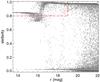 |
Fig. 20 Stellarity parameter as a function of r′ band magnitude derived from the CFHT data. It can be clearly seen that the stellarity parameters are mostly either close to 1 or 0 unless the sources are very faint. Note that the sources brighter than 16 mag have relatively small stellarities because the central parts of their images are saturated. |
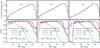 |
Fig. 21 Source counts of NIR bands and the matching ratio against optical and other NIR bands. Top panels show the distribution of sources as a function of magnitude per square degree per 0.2 mag bin. In the lower panels, the matching ratio against those in other NIR bands and optical data are presented together. |
6.1. Number counts and the source matching ratio
We present number counts for each band and the cross-matching rate of the sources against optical data and the other bands as a function of magnitude. Figure 21 shows the results for the NIR bands. The top panels show the number counts of NIR band sources which are confirmed through the cross-checking process with the other bands. The N2 sources brighter than 12.6 mag were excluded during the data reduction process because they were heavily saturated and generated MUXbleeds. We found that the sources with no counterparts in the other data are mostly fainter than 19 mag in the N2 band. On the other hand, most of the false objects at bright magnitudes were found to be residual streaks around bright stars through the visual inspection of the image. On the other hand, at fainter magnitudes, most of the false objects close to the detection limits are due to noises, because the comparison of common areas of the NEP-Deep and NEP-Wide data shows that many of these faint sources do not appear as real sources in the NEP-Deep, whose detection limits are more than 1 mag deeper.
In the lower panel, we show the matching ratios against the optical, and the other two NIR bands data separately. The fraction of sources for which the stellarity is greater than 0.8 without any constraint on magnitude are indicated by the gray line in this panel. The fraction of star-like objects that are defined as those with the optical stellarity greater than 0.8 and r magnitude brighter than 19 are shown as blue dotted lines. Using the optical-IR SEDs of these objects, we confirmed that most of the star-like objects closely follow black body spectra, suggesting that they are indeed likely to be stars. Figure 21 thus suggests that the sources brighter than 14 mag in the N2 band are mostly stars, even though the actual number of them is small. The fraction of high-stellarity objects rapidly decreases around 17 mag, and completely falls off to zero toward ~20 mag. The features in the N3 and N4 band are generally similar to those in the N2 band. The properties of these objects in color–color diagrams are discussed in the following subsection. The overall fraction of star-like objects among the entire N2 sources is about 17%. In the N3 and N4 bands, these fractions are about 15% and 16%, respectively.
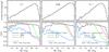 |
Fig. 22 Same as Fig. 21, but for the MIR-S band sources. The top panel shows the number of sources per square degree per 0.2 mag bin as a function of magnitude. In the lower panel, the matching rates of the sources against those in the other MIR-S bands and the optical data are presented together with the fraction of star-like sources. |
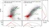 |
Fig. 24 Color–color diagrams of the NEP-Wide NIR sources matching with optical data. a) (N2 − N3) vs. (N3 − N4) color and b) (N2 − N3) vs. (N2 − N4) color. Dark dots represent all of the sources having optical counterparts and red dots represent the “star-like” sources defined as having the criteria of stellarity >0.8 and r′ < 19. The histograms in both the right and lower panels show the number of sources per 0.2 mag bin. |
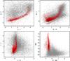 |
Fig. 25 Color–color diagrams and color-magnitude diagram of the NEP-Wide sources matched with the optical data. They show the various colors by optical bands from the CFHT and Maidanak and the NIR J, H bands. Red dots represent the “star-like” sources defined as having stellarity >0.8 and r′ < 19. |
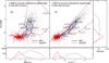 |
Fig. 26 Color–color diagrams of the NEP-Wide MIR source matching with optical data. a) (S7 − S9W) vs. (S9W − S11) and b) (S7 − S9W) vs. (S7 − S11) color–color diagrams. All of the MIR sources having optical counterparts are presented using dark dots in the diagrams. Among them, the star-like sources defined as those with stellarity greater than 0.8 are indicated by the red histogram. |
The same analysis was conducted for the MIR bands and the results are shown in Fig. 22 (MIR-S) and 23 (MIR-L). The numbers of sources detected in the MIR bands are much smaller than those in the NIR bands. Compared to the fraction of high-stellarity sources in the NIR bands, their fractions in the MIR bands are small at all magnitudes, and decreases significantly toward the longer wavelength bands. However, the number of these sources neither rapidly decline nor become zero in the fainter regions.
Overall, about 22% of the entire NIR and 20% of the MIR sources do not have optical counterparts within a 3′′ radius, while there are multiple optical counterparts for some sources. This multiple matching was most serious between the optical and MIR band sources. We found multiple optical counterparts for about 17% of the MIR sources during the MIR band merging. In these cases, we tried to identify the proper counterparts using the optical sources that had NIR counterparts from AKARI or in the J, H bands. Through this process, we were able to assign the reliable counterparts with confidence. Despite this, the nearest neighbor does not seem to be the most likely optical counterpart for about (~3%) of the MIR sources. In those cases, we visually inspected the images, although this provided little help. In the final catalog, all of the optical counterparts are indeed those found to be the nearest neighbors.
6.2. Color–color and color–magnitude diagrams
It is not easy to clearly establish the nature of the sources with the AKARI data alone. We attempted to distinguish different types of sources using various color-magnitude and color–color diagrams.
The star-like sources are plotted with red colors in each color–color diagram from Figs. 24 to 27. The color–color diagrams for the three NIR bands of AKARI are shown in Fig. 24. The majority of the star-like sources lie in the narrow range of colors of −0.7 < (N2 − N3) < −0.4, −1.5 < (N2−N4) < −1.0 and −0.9 < N3 − N4 < −0.4. The sources with stellarity greater than 0.95, magnitudes in the range 14.5 < r < 17.5, and identified as stellar sources by inspection of their images and SEDs are overplotted in dark red. We also present various optical-NIR color–color diagrams in Fig. 25. The star-like sources form a tight sequence in the (g′ − z′) versus (u′ − r′) color–color diagram, being located along the lower right edge. On the other hand, extended sources are more widely spread, occupying the entire region above the stellar-source sequence. In the (R − I) versus (B − R) color–color diagrams, however, the stellar sequence is somewhat broad and runs across the broader region occupied by the extended sources. The NIR colors such as (J − H) and (H − N2) are also useful in distinguishing the stars from galaxies (extended sources) as shown in the lower panels of Fig. 25. The (J − N2) color is not shown here but it is similar to the (H − N2) color. The N2 vs. (H − N2) color–magnitude diagram (CMD) in the last panel shows that the star-like sources are the brightest ones in the N2 band. By comparing these properties in color–color plots, we can separate stars effectively, even though we are unable to identify all stars individually. The diagrams show that the high-stellarity sources are statistically good indicator for the selection of the stars although the criterion does not perfectly identify stars in all cases.
The colors of galaxies provide us with valuable information about their composition and history (Fukugita et al. 1995). However, unlike point sources, extended sources show widely spread across the color–color diagrams as shown in Figs. 24 to 27. In Fig. 24, we have plotted the redshift tracks of the templates (Silva et al. 1998) of the star-forming galaxy M51 and the typical ultra-luminous infrared galaxy (ULIRG) Arp220 over the diagrams. Compared to these tracks, we find that the NEP-Wide sources are located close to the redshift sequence, although the scatter is quite large. This could mean that the galaxy SEDs are quite diverse, but in addition, a large fractions of the NEP-Wide sources are star forming galaxies at different redshifts. About 70% of the MIR-selected sources in AKARI’s early data were identified as star forming galaxies through the detailed inspection of their infrared SEDs (Lee et al. 2007). Since the NIR parts of the SEDs of star-forming galaxies are dominated by late-type stars and thus rather homogeneous, the NIR colors are mostly determined by the galaxy redshifts. The histograms show the distribution of the source density in each 0.1 mag bin. We also note that many sources are located quite far away from the star forming galaxy sequence. Some of these sources with very red NIR colors are likely to be active galactic nuclei (AGNs; Lee et al. 2007).
In Figs. 26 and 27, we show the diagrams using the colors for the MIR bands, for which, the NEP-Wide sources appear to have a much wider distribution. As for the sources used in the previous color–color diagrams, optically matched sources are presented with gray colors and the star-like sources are plotted with red colors. As shown in these figures, the MIR-S color–color diagrams (S7−S9W), (S7−S11) and (S9W−S11) show that the star-like sources are well segregated from the other sources, but this feature gradually disappears in the longer wavelength band colors. Most of the stars (and the early type galaxies) detected in the NIR bands seem to fade out in the MIR bands. Unlike the NIR and MIR-S band colors, the MIR-L band colors do not seem to be helpful in classifying stars since the MIR-L band color–color diagrams do not show any prominent features. The variation in the NIR colors are mainly due to the wide range of galaxy redshift, while the MIR colors are sensitive to the star formation rates, causing the wide spread in the MIR color–color diagrams. The number of sources detected in all IRC bands is about 1000 and most of them seem to be late-type star forming galaxies. Many of these are identified as disk galaxies by the visual inspection of the optical images, and from their optical-IR SEDs. They are not located in a particular region and occupy a large area in the color–color diagrams. However, various interesting sources seem to be included in the all-band detected sources. Bright sources in the MIR-L bands that have radio counterparts are likely to be AGNs (Lee et al. 2009). We found that many of them show a power law distribution of SEDs while some show PAH bumps (Takagi et al. 2010). Dozens of sources are bright (<17 mag) in either the L18W or L24 band and have faint optical (r′ or R) counterparts, seemingly suspected to be dust obscured galaxies (DOGs), a class of high-redshift ULIRGs. There are no sources with high-stellarity associated with faint MIR-L sources. In addition, the MIR-L sources detected in only one band, having no counterparts in our other data sets seem possibly to be very red objects.
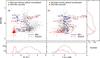 |
Fig. 27 a) (N2 − N3) vs. (S7 − S11), and b) (N2 − N3) vs. (L15 − L18W) color–color diagrams. The NEP-Wide sources whose optical stellarities are known by cross-matching with the optical CFHT and Maidanak catalogs are presented using dark dots in the diagrams. Among them, the star-like sources are plotted in red. |
7. Summary and conclusion
We have carried out the reduction and analysis of the NEP-Wide survey data obtained by the AKARI/IRC. In order to reduce spurious detection, we masked out the regions affected by instrumental effects such as MUXbleeding trails, especially in the NIR bands. The detected sources were compared with the available data at other wavelengths, including optical, ground-based NIR observations, in addition to the other bands of AKARI. The areal coverage is about a 5.4 deg2 circular field centered on the NEP. The 5σ detection limits of the survey are around 21 AB mag in the NIR bands, 19–19.5 mag in the MIR-S bands, and 18.5–18.8 mag in the MIR-L bands.
The ancillary optical data from the CFHT and the Maidanak observatory are sufficiently deep to identify most of the AKARI sources. We carried out extensive comparisons by cross-matching of the sources among the photometric bands ranging from optical to MIR wavelengths in order to confirm the validity of the detected sources and exclude the low-reliability sources. Using these results, we produced a band-merged source catalog covering the wavelength bands from the u∗ band to the MIR L24 band. This catalog contains about 114 800 entries. On the basis of this catalog, we have shown the characteristics of the sources using various color–color diagrams. By comparing and using optical stellarity, we found that the NIR and MIR-S band colors provide a reliable means of distinguishing stars from galaxies. Except for the star-like objects, most of the NEP-Wide sources appear to be various types of star forming galaxy. The sources detected in all of the AKARI/IRC bands include interesting sources such as PAH galaxies, AGNs, ULIRGs, DOG candidates, or MIR-bright early-type galaxies.
The NEP-Wide catalog covers a moderately large sky area with a wide wavelength range. It complements the NEP-Deep catalogs of Wada et al. (2008) and Takagi et al. (2012), which have better sensitivity and smaller angular coverage, but the same filter bands.
The Spitzer space telescope has also carried out large area surveys such as the Spitzer Wide-Area Infrared Extragalactic (SWIRE) Survey and First Look Survey (FLS). These surveys are carried out with all wide-band filters of Spitzer: 3.6 4.5, 5.8, and 8.0 μm with the Infrared Array Camera (IRAC) and 24, 70, and 160 μm with the Multiband Imaging Photometer for Spitzer (MIPS). This should be compared to the nearly continuous wavelength coverage of AKARI’s NEP surveys from 2.4 to 24 μm. The FLS covered the area of about 5 deg2, which is similar to that of the NEP-Wide. The survey area of SWIRE is about ten times larger, but composed of several different fields.
IRAF is distributed by the National Optical Astronomy Observatories, which are operated by the Association of Universities for Research in Astronomy, Inc., under cooperative agreement with the National Science Foundation.
This software is accessible at AKARI observers web page (http://www.ir.isas.jaxa.jp/AKARI/Observation).
There are imaging version and spectroscopic version for IRAF users.
For the detailed description of this software, see http://terapix.iap.fr/IMG/pdf/sextractor.pdf
Acknowledgments
This work is based on observations with AKARI, a JAXA project with the participation of ESA, universities and companies in Japan, Korea, the UK, and Netherlands. This work contains many data obtained by the ground-based Maidanak Observatory’s 1.5 m, KPNO 2.1 m, and CFHT 3.5 m telescopes. This work was supported by the Korean Research Foundation grant 2006-341-C00018. A.S. and A.P. have been supported by the research grant of the Polish National Science Centre N N203 51 29 38.
References
- Bertin, E., & Arnouts, S. 1996, A&AS, 117, 393 [NASA ADS] [CrossRef] [EDP Sciences] [Google Scholar]
- Fukugita, M., Shimasaku, K., & Ichikawa, T. 1995, PASP, 107, 945 [NASA ADS] [CrossRef] [Google Scholar]
- Holloway, H. 1986, J. Appl. Phys., 60, 1091 [NASA ADS] [CrossRef] [Google Scholar]
- Hwang, N., Lee, M. G., Lee, H. M., et al. 2007, ApJS, 172, 583 [NASA ADS] [CrossRef] [Google Scholar]
- Im, M., Ko, J., Cho, Y., et al. 2010, J. Korean Astron. Soc., 43, 75 [Google Scholar]
- Jeon, Y., Im, M., Ibrahimov, M., et al. 2010, ApJS, 190, 166 [NASA ADS] [CrossRef] [Google Scholar]
- Kawada, M., Baba, H., Barthel, P. D., et al. 2007, PASJ, 59, S389 [NASA ADS] [CrossRef] [Google Scholar]
- Kollgaard, R. I., Brinkmann, W., Chester, Margaret, M., et al. 1994, ApJS, 93, 145 [NASA ADS] [CrossRef] [Google Scholar]
- Kron, R. G. 1980, ApJS, 43, 305 [NASA ADS] [CrossRef] [Google Scholar]
- Lacy, M., Miley, J. M., Waldram, E. M., et al. 1995, MNRAS, 276, 614 [NASA ADS] [CrossRef] [Google Scholar]
- Lee, H. M., Im, M., Wada, T., et al. 2007, PASJ, 59, S529 [NASA ADS] [Google Scholar]
- Lee, H. M., Kim, S. J., Im, M., et al. 2009, PASJ, 61, 375 [NASA ADS] [Google Scholar]
- Lorente, R., Onaka, T., Ita, Y., et al. 2008, AKARI IRC Data User Manual, ver. 1.4 [Google Scholar]
- Matsuhara, H., Wada, T., Matsuura, S., et al. 2006, PASJ, 58, 673 [NASA ADS] [Google Scholar]
- Murakami, H., Baba, H., Barthel, P., et al. 2007, PASJ, 59, S369 [NASA ADS] [CrossRef] [MathSciNet] [Google Scholar]
- Offenberg, J., Fixen, D. J., Rauscher, B. J., et al. 2001, PASP, 113, 240 [NASA ADS] [CrossRef] [Google Scholar]
- Oke, J. B., & Gunn, J. E. 1983, ApJ, 266, 713 [NASA ADS] [CrossRef] [Google Scholar]
- Onaka, T., Matsuhara, H., Wada, K., et al. 2007, PASJ, 59, S401 [NASA ADS] [Google Scholar]
- Polletta, M., Tajer, M., & Maraschi, L., et al. 2007, ApJ, 663, 81 [NASA ADS] [CrossRef] [Google Scholar]
- Skrutskie, M. F., Curtie, R. M., Stiening, R., et al. 2006, AJ, 131, 1163 [NASA ADS] [CrossRef] [Google Scholar]
- Sedgwick, C., Serjeant, S., Sirothia, S., et al. 2009, ASPC, 418, 519 [NASA ADS] [Google Scholar]
- Shim, H., Im, M., Lee, H. M., et al. 2011, ApJ, 727,14 [NASA ADS] [CrossRef] [Google Scholar]
- Silva, L., Granato, G. L., Bressan, A., et al. 1998, ApJ, 509, 103 [NASA ADS] [CrossRef] [Google Scholar]
- Tanabe, T., Sakon, I., Cohen, M., et al. 2008, PASJ, 60, S375 [NASA ADS] [CrossRef] [Google Scholar]
- Takagi, T., Oyama, Y., Goto, T., et al. 2010, A&A, 514, A5 [NASA ADS] [CrossRef] [EDP Sciences] [Google Scholar]
- Takagi, T., Matsuhara, H., Goto, T., et al. 2012, A&A, 537, A24 [NASA ADS] [CrossRef] [EDP Sciences] [Google Scholar]
- van Dokkum, P. G. 2001, PASP, 113, 1420 [NASA ADS] [CrossRef] [Google Scholar]
- Wada, T., Oyabu, S., Ita, Y., et al. 2007, PASJ, 59, S515 [NASA ADS] [Google Scholar]
- Wada, T., Matsuhara, H., Oyabu, S., et al. 2008, PASJ, 60, S517 [NASA ADS] [Google Scholar]
- White, G. J., Perason, C., Braun, R., et al. 2010, A&A, 517, A54 [NASA ADS] [CrossRef] [EDP Sciences] [Google Scholar]
All Tables
All Figures
|
Fig. 1 Overall map of the NEP-Wide field. The survey consisted of 446 pointing observations represented by green boxes. Each frame covered a 10′ × 10′ area with half of its field of view (FoV) overlapped by neighboring frames. The red box and blue lines represent the regions covered by optical surveys at the CFHT and Maidanak Observatory, respectively. The circular gray-shaded region denotes the NEP-Deep field. |
| In the text | |
|
Fig. 2 Overall view of the observation template IRC03, which was used for NEP-Wide observations. For one pointing observation, the exposure was carried out according to a fixed sequence. The structure of the raw data obtained in the IRC03 mode are shown in the bottom panel. The NIR data consist of one short and one long-exposure, whereas the MIR data are composed of one short- and three long-exposures. |
| In the text | |
|
Fig. 3 Schematic view of the procedures in the pipeline designed for the preprocessing of the IRC imaging data. The imaging pipeline is composed of three parts. |
| In the text | |
|
Fig. 4 Schematic flow chart describing the iterative procedures used to find a satisfactory solution for the WCS header of the L18W and L24 band data. |
| In the text | |
|
Fig. 5 Example showing the result of cosmic-ray rejection. The left panel a) is a sample portion of the N4 image produced by the IRC imaging pipeline (PID: 2100757) on which many cosmic rays remain. The middle panel b) is the same image restored by cosmic-ray rejection using the L.A. cosmic procedure. The third panel c) shows the result of subtraction, a–b, which is just a map showing the rejected cosmic rays. |
| In the text | |
|
Fig. 6 Close-up views of a sample region around bright sources showing false detections at each NIR band caused by MUX-bleeding trails before the correction. The left, middle, and right panels show the N2, N3, and N4 band images, respectively. Colored circles indicate the objects that were not matched with optical data. |
| In the text | |
|
Fig. 7 Schematic diagram describing the procedures used to make a weight map for an individual frame obtained from a single pointing observation. The first panel a) is a sample image containing a bleeding trail and a bright source whose center is disrupted. The second panel b) shows the regions to be masked. The third panel c) represents the number of rejected frames during the stacking procedure. Each pixel has an integer value ranging 0 to 3. The last panel d) is a weight map to be used for the final mosaicking procedure. |
| In the text | |
|
Fig. 8 Segments of mosaic images (left) and weighted coverage maps (right) before and after the MUXbleed correction (N3). The upper pair shows the images before this process and the bottom panels show them after the operation. The bleeding trails in this field are completely removed by this weighted mosaicking method using weight maps. In the map d), zero-weighted pixels are in black. |
| In the text | |
|
Fig. 9 Entire coverage maps of the NIR data before (upper) and after (lower) the correction for MUX bleeds. Uncovered area and none-weighted pixels have zero values (white area), which have wedge-like shape from the center to radially outer direction. |
| In the text | |
|
Fig. 10 Entire coverage maps of MIR-S (upper) and MIR-L (lower) bands. |
| In the text | |
|
Fig. 11 Segments of a mosaic images (left) and weighted coverage maps (right) before and after the correction for undesirable patterns in the S9W image. The upper panels show the images before the masking and the bottom panels show the resultant images after masking. Coverage maps show that the masking of MIR-S images effectively removes most of the remaining patterns (for 19 frames), and demonstrates that remaining MUXbleed effects are almost completely removed. |
| In the text | |
|
Fig. 12 Completeness estimation for each band (red curves). The estimates for the NEP-Deep data are also shown for comparison. The gray histograms show the NEP-Wide source density per square degree per 0.2 mag bin at each band (not corrected for incompleteness). |
| In the text | |
|
Fig. 13 Flux detection limits and 50% completeness limits for each band. The detection limits of the NIR bands are around 21 mag, and MIR bands reach much shallower depth than NIR bands. The 50% completeness limits are about 1.2 mag shallower than the detection limits in the NIR filters and about 0.7 mag shallower in the MIR bands from S7 to L18W. |
| In the text | |
|
Fig. 14 Probability of random matching for the N2 band sources with those in other bands. The random matching probability is proportional to the density of the sources in the band to be matched, as indicated by the dotted line. |
| In the text | |
|
Fig. 15 Summary of the source matching between the different NIR bands. The numbers of sources detected in each NIR band are presented at the apexes of the triangle. The matching results amongst them are shown, excluding any duplicated or multiply matched sources. The numbers in the dotted ellipses represent the number of sources with detections in both of the matching bands. |
| In the text | |
|
Fig. 16 Schematic diagram showing the results of the matching between the sources in the NIR and MIR bands except for multiply matched sources. The matching results of the N2 sources with all the MIR bands are shown in the leftmost panel. The results for N3 and N4 bands are shown in the middle and the right panels, respectively. |
| In the text | |
|
Fig. 17 Results of the matching AKARI sources with the optical data covering two separate fields of the CFHT and Maidanak observations. On the left and right of the diagram, the results for the CFHT and Maidanak data are presented, respectively. Overall results of the matching both sets of optical data are given in the bottom of the figure. |
| In the text | |
|
Fig. 18 Number of sources in each of the NIR band detection catalogs matched with KPNO J, H band data. About 78%, 63%, and 65% of the N2, N3, and N4 sources were found to have counterparts in the J and H band data. |
| In the text | |
|
Fig. 19 Schematic diagram describing the band merging procedure. we first combined the three catalogs of the NIR, MIR-S, and MIR-L channels. We then merged them into a band-merged catalog covering the optical u∗ to the L24 band. During this procedure, we checked the source IDs carefully in order to avoid any duplication of the same entries. |
| In the text | |
|
Fig. 20 Stellarity parameter as a function of r′ band magnitude derived from the CFHT data. It can be clearly seen that the stellarity parameters are mostly either close to 1 or 0 unless the sources are very faint. Note that the sources brighter than 16 mag have relatively small stellarities because the central parts of their images are saturated. |
| In the text | |
|
Fig. 21 Source counts of NIR bands and the matching ratio against optical and other NIR bands. Top panels show the distribution of sources as a function of magnitude per square degree per 0.2 mag bin. In the lower panels, the matching ratio against those in other NIR bands and optical data are presented together. |
| In the text | |
|
Fig. 22 Same as Fig. 21, but for the MIR-S band sources. The top panel shows the number of sources per square degree per 0.2 mag bin as a function of magnitude. In the lower panel, the matching rates of the sources against those in the other MIR-S bands and the optical data are presented together with the fraction of star-like sources. |
| In the text | |
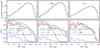 |
Fig. 23 Same as Fig. 22, but for the MIR-L band sources. |
| In the text | |
|
Fig. 24 Color–color diagrams of the NEP-Wide NIR sources matching with optical data. a) (N2 − N3) vs. (N3 − N4) color and b) (N2 − N3) vs. (N2 − N4) color. Dark dots represent all of the sources having optical counterparts and red dots represent the “star-like” sources defined as having the criteria of stellarity >0.8 and r′ < 19. The histograms in both the right and lower panels show the number of sources per 0.2 mag bin. |
| In the text | |
|
Fig. 25 Color–color diagrams and color-magnitude diagram of the NEP-Wide sources matched with the optical data. They show the various colors by optical bands from the CFHT and Maidanak and the NIR J, H bands. Red dots represent the “star-like” sources defined as having stellarity >0.8 and r′ < 19. |
| In the text | |
|
Fig. 26 Color–color diagrams of the NEP-Wide MIR source matching with optical data. a) (S7 − S9W) vs. (S9W − S11) and b) (S7 − S9W) vs. (S7 − S11) color–color diagrams. All of the MIR sources having optical counterparts are presented using dark dots in the diagrams. Among them, the star-like sources defined as those with stellarity greater than 0.8 are indicated by the red histogram. |
| In the text | |
|
Fig. 27 a) (N2 − N3) vs. (S7 − S11), and b) (N2 − N3) vs. (L15 − L18W) color–color diagrams. The NEP-Wide sources whose optical stellarities are known by cross-matching with the optical CFHT and Maidanak catalogs are presented using dark dots in the diagrams. Among them, the star-like sources are plotted in red. |
| In the text | |
Current usage metrics show cumulative count of Article Views (full-text article views including HTML views, PDF and ePub downloads, according to the available data) and Abstracts Views on Vision4Press platform.
Data correspond to usage on the plateform after 2015. The current usage metrics is available 48-96 hours after online publication and is updated daily on week days.
Initial download of the metrics may take a while.