| Issue |
A&A
Volume 543, July 2012
|
|
|---|---|---|
| Article Number | A19 | |
| Number of page(s) | 15 | |
| Section | Extragalactic astronomy | |
| DOI | https://doi.org/10.1051/0004-6361/201219091 | |
| Published online | 21 June 2012 | |
Galaxy mass, cluster-centric distance and secular evolution: their role in the evolution of galaxies in clusters in the last 10 Gyr
INAF – Osservatorio Astronomico di Brera, via Brera 28, 20121 Milan, Italy
e-mail: This email address is being protected from spambots. You need JavaScript enabled to view it.
; This email address is being protected from spambots. You need JavaScript enabled to view it.
Received: 22 February 2012
Accepted: 15 May 2012
Abstract
Context. Galaxy mass and environment are known to play a key role in galaxy evolution: studying galaxy colors as a function of redshift, galaxy mass, and environment offers a powerful diagnosis to disentangle the role of each.
Aims. We study the simultaneous dependence of the fraction of blue galaxies fblue on secular evolution, environment, and galaxy mass with a well-controlled cluster sample. We are thus able to study the evolution and respective role of the cessation of star formation history (SFH) in clusters caused by galaxy mass (“mass quenching”) or by environment (“environmental quenching”).
Methods. We defined an homogenous X-ray selected cluster sample (25 clusters with 0 < z < 1 and one cluster at z ~ 2.2), having similar masses and well-defined sizes. Using multicolor photometry and a large spectroscopic sample to calibrate photometric redshifts, we carefully estimated fblue for each cluster at different galaxy mass and cluster-centric distance bins. We then fitted the dependence of fblue on redshift (z), environment (r/r200) and galaxy mass (M) with a simple model.
Results.fblue increases with cluster-centric distance with a slope α = 1.2-0.3+0.4, decreases with galaxy mass with a slope β = -3.8-0.5+0.6, and increases with redshift with a slope γ = 3.3-0.6+0.7. The data also require for the first time a differential evolution with galaxy mass of fblue with redshift, with lower mass galaxies evolving slower by a factor ζ = -3.9-1.1+0.9.
Conclusions. Our study shows that the processes responsible for the cessation of star formation in clusters are effective at all epochs (z ≲ 2.2), and more effective in denser environments and for more massive galaxies. We found that the mass and environmental quenchings are separable, that environmental quenching does not change with epoch, and that mass quenching is a dynamical process, i.e. its evolutionary rate is mass-dependent. Our study extends the downsizing-like scenario, where the most massive galaxies have their properties set at a very high redshift, to the cluster environment and all galaxies. It illustrates the need to disentangle galaxy mass and cluster-centric distance to properly estimate the behavior of fblue in clusters.
Key words: galaxies: clusters: general / galaxies: clusters: individual: JKCS 041 / galaxies: evolution / galaxies: star formation
© ESO, 2012
1. Introduction
It is well-established that galaxy mass and environment are key parameters in shaping galaxy properties (e.g., Butcher & Oemler 1978; Dressler 1980; De Propris et al. 2003). At least in the local Universe, both change galaxy properties in a similar direction, for instance making them preferentially redder (e.g., Visvanathan & Sandage 1977; Butcher & Oemler 1978) or of early-type morphology (e.g., Blanton et al. 2003; Dressler 1980). Furthermore, there is a correlation between galaxy mass and environment, because denser environments tend to be inhabited by more massive galaxies (e.g., Hogg et al. 2003; Baldry et al. 2006). In the local Universe, the Sloan Digital Sky Survey (SDSS, York et al. 2000) provided data from which one could quantify the role of each to an unprecedented precision (e.g., Kauffmann et al. 2004; Peng et al. 2010).
However, when considering higher redshifts (z ~ 1–2), the analysis is complicated – and additionally there are less data available – by the disentangling of the precise role of secular galaxy evolution, of galaxy mass, and of environment on galaxy properties. Therefore, any analysis of galaxy evolution at z ~ 1–2 needs to simultaneously control for galaxy secular evolution, galaxy mass, and environment. Indeed, any bias in one of those three terms may confuse the interpretation of the obtained result. For instance, a blueing related to a younger age at higher redshift may be mistaken for a blueing induced by a sampling biased preferentially toward lower density environments, which are richer in blue galaxies.
Controlling for galaxy mass requires working with galaxy mass-selected samples, which presents the advantage of a better control of the sample. Indeed, galaxy mass has on average a much more regular evolution (increasing with decreasing redshift) than galaxy rest-frame optical luminosity, which can temporarily increase with starbust, and then decrease. For example, a sample selected on rest-frame optical luminosity is very likely to be biased toward those temporary low-mass starbust galaxies at high redshifts, thus introducing a spurious increase in the fraction of blue galaxies that disappears if a mass-selected sample is used (e.g., De Propris et al. 2003). A more subtle question is the mass evolution of star-forming galaxies that will significantly increase their stellar mass with time. For example, an average star formation rate of 2 M⊙ yr-1 (resp. 5 M⊙ yr-1) for 5 Gyr (resp. 2 Gyr) is sufficient to build 1010 M⊙. Therefore, selecting galaxies by stellar mass measured at the galaxy redshift may introduce a net inflow with decreasing redshift of galaxies that rise above the mass threshold adopted for the study. This uncontrolled inflow with decreasing redshift of galaxies in the selected sample leaves the ambiguity between a real evolution of massive blue galaxies and a selection effect. To remove this ambiguity, one needs to control for mass not at the redshift of observation, but evolved at z = 0 to select at high redshift the likely ancestors of present-day galaxies of a given mass (e.g., Andreon et al. 2008; Raichoor & Andreon 2012).
Controlling for secular evolution requires acknowledging that the galaxy rest-frame color evolves with time. Indeed, galaxies observed at higher redshifts will on average have bluer rest-frame colors than their local counterparts, because of their mean younger age and of the higher mean star formation activity of the Universe at higher redshifts (e.g., Lilly et al. 1996; Madau et al. 1998). Using a non-evolving rest-frame color will classify an increasing number (with increasing redshift) of red-sequence galaxies as blue galaxies, thus possibly introducing a spurious evolutionary trend. One can take this into account by using evolving rest-frame colors to characterize galaxy properties at different redshifts, as proposed by Andreon et al. (2006) and now adopted in several works (e.g., Haines et al. 2009; Peng et al. 2010; Raichoor & Andreon 2012).
Controlling for environment raises the question of how to measure environment. Available data often oblige us to use a proxy for an environment estimate based on samples with either photometric redshift or that are rest-frame B-band luminosity-selected. However, at z ~ 1–2, these proxies may be either prone to large uncertainties or potentially biased toward (temporarily) blue overdensities. Again, this may introduce spurious trends or smooth existing ones (for instance, see discussion in Sect. 3 of Quadri et al. 2012). In this regard, clusters of galaxies are ideal laboratories. On the one hand, their cores unambiguously represent the densest environment in the Universe at each epoch, where environmental processes consequently are the most effective. On the other hand, they provide, at fixed redshift, handy samples of galaxies observed in similar conditions, with little contamination. Nevertheless, when using cluster-centric distance as the environment’s measurement in clusters, one should scale it with the cluster size (e.g. r200): if not, one risks to assign the same environmental measurement to different physical environments, thus mixing age-related trend (redshift dependence) with environmental trend. The effect is of paramount importance because gradients in cluster populations are usually important. For instance, if one probes a cluster region within a fixed radius (e.g. 1 Mpc), one will probe only central regions of large clusters but outer regions for small clusters, which possibly introduces an artificial dependence with respect to the cluster size (e.g. Margoniner et al. 2001). Moreover, even if challenging at z ~ 1–2, a robust cluster size estimation is needed to prevent any smoothing of possible environmental trends when co-adding data (see for instance Loh et al. 2008, and the use of the approximate cluster size estimate BGC).
Additionally, if one uses galaxy clusters to study galaxy evolution, the cluster selection function should be as independent as possible of the (studied) galaxy population. As an example, by selecting preferentially clusters rich in blue galaxies at higher redshift (because they are easier to detect, as in the early 80’s, Kron 1995) or richer in red galaxies (because clusters are detected thanks to the red sequence, as in Loh et al. 2008, with the RCS) likely introduces a selection effect when estimating the fraction of blue galaxies (Andreon et al. 2006). It is preferable to select clusters by their X-ray emission, because at a given X-ray emission (LX or TX) clusters rich in blue galaxies are not favored/disfavored at a given cluster mass (Andreon & Ettori 1999). Furthermore, it is well-known that cluster galaxy properties depend on the cluster richness (e.g., Oemler 1974; Dressler 1980; Dressler et al. 1997; Hansen et al. 2009): a way to control this dependence is to select clusters with similar masses.
In this paper, we aim at disentangling the role of galaxy secular evolution, galaxy mass, and environment on galaxy evolution by analyzing a cluster sample spanning a wide redshift baseline. An observationally economic but still physically efficient proxy for measuring the star formation activity is galaxy color (e.g., Butcher & Oemler 1984; Williams et al. 2009; Peng et al. 2010). We classified galaxies into two broad categories (blue or red) and defined the fraction of blue galaxies fblue at a given galaxy mass M and scaled cluster-centric distance r/r200, in the vein of the pioneering work of Butcher & Oemler (1984). In the last decades, numerous works studied fblue in clusters (e.g., De Propris et al. 2003; Andreon et al. 2006; Loh et al. 2008; Haines et al. 2009, to name a few) but none of them studied the dependence of fblue on redshift, galaxy mass, and cluster-centric distance at the same time. Analyzing simultaneously the dependence of fblue on those three parameters allows one to put strong constraints on the various processes that are responsible for the cessation of star formation activity (“quenching”).
To achieve this, we considered the aforementioned remarks to our best ability. We used a sizable X-ray selected cluster sample (25 clusters with 0 < z < 1 and the JKCS 041 cluster at z ~ 2.2) with well-defined r200 and similar cluster masses, thus minimizing the correlation between fblue and our cluster selection function. We then estimated fblue as a function of galaxy mass M and scaled cluster-centric distance r/r200, defining blue/red galaxies considering also the stellar evolution of galaxies with time. To lead the analysis, we used a reasonable evolutionary model as a reference (exponentially declining star formation history, fixed formation redshift), and then measured any deviation from this reference. This reference model does not aim to describe the individual behavior of each galaxy, but to cancel out overall trends such as stellar aging or stellar mass increasing with time. Deviations from this reference model highlight the evolution and respective role of the quenching in clusters caused by galaxy mass or by environment.
The plan of this paper is as follows. We define in Sect. 2 the cluster sample on which this study relies. Section 3 presents the data and their analysis, including our estimation of fblue. Our results are presented in Sect. 4 and are summarized and discussed in Sect. 5. We adopt H0 = 70 km s-1 Mpc-1, Ωm = 0.30, and ΩΛ = 0.70 throughout. All magnitudes are in the AB system, corrected for Galactic extinction using Schlegel et al. (1998). Masses are computed with a Chabrier (2003) initial mass function and, if not stated otherwise, are defined by the mass of the gas that will eventually be turned into stars, i.e. corresponding to the integral of the star formation rate.
2. Cluster sample
We describe in this section our cluster sample. It was assembled from an X-ray selection and clusters with similar masses at different redshifts, using the cluster X-ray temperature as mass proxy. The X-ray selection ensures that our cluster sample selection is unbiased by fblue, because the probability of inclusion of a cluster in the sample is independent of fblue at a given cluster mass. At intermediate redshift, we relied on the X-ray selected cluster sample from the first five deg2 of the XMM Large-Scale Structure survey (XMMLSS, Pierre et al. 2004). At low redshift, we extracted a sample from the HIghest X-ray FLUx Galaxy Cluster Sample (HIFLUGCS, Reiprich & Böhringer 2002), an X-ray selected cluster sample, by selecting clusters with comparable cluster masses. We added to this sample the JKCS 041 cluster (z ~ 2.2, Andreon et al. 2009; Andreon & Huertas-Company 2011). Though this cluster is different from the other objects, because it is not X-ray selected, it is the highest redshift cluster with a significant X-ray emission; moreover, its mass/temperature is comparable to the rest of our sample. Figure 1 displays the temperature TX of our cluster sample as a function of redshift. We note that our clusters (except for JKCS 041) have kT ~ 3 keV, typical of intermediate mass clusters. We have r200 for all the objects, which is of paramount importance, because it is known that fblue depends on cluster-centric distance. It has been derived from TX or σv as described in Appendix A. The properties of the clusters are listed in Table 1.
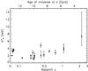 |
Fig. 1 TX as a function of redshift for our cluster sample. |
Cluster sample.
2.1. XMMLSS sample (0.14 ≤ z ≤ 1.05)
The main body of our cluster sample comes from the XMMLSS. This survey is located in the W1 area of the Canada-France-Hawaii Telescope Legacy Survey (CFHTLS), which provides u∗g′r′i′z′-band data. More precisely, we selected all clusters from the first five deg2 (Valtchanov et al. 2004; Willis et al. 2005; Pacaud et al. 2007), which are in the CFHTLS W1 field (see Fig. 2). We removed clusters with lower-than-average data quality: XLSSC 011 and XLSSC 021 (their galaxies saturate CFHTLS W1 data because they are too nearby), XLSSC 004 (no TX or σv measurements, so we cannot estimate r200), XLSSC 017 and XLSSC 020 (located where CFHTLS W1 data are corrupted), XLSSC 022 (blended with clusters at similar redshifts). We finally assembled 18 clusters, 15 of which having r200 estimated from TX measurements with the XMM-Newton telescope (Pacaud et al. 2007), 3 (XLSSC 007, XLSSC 014, and XLSSC 016) from σv measurements (Willis et al. 2005).
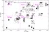 |
Fig. 2 CFHTLS W1 cluster subsample: spatial location of the 18 clusters of our CFHTLS W1 subsample (red crosses). The magenta dashed lines represents CFHTLS W1 fields. For each cluster, blue circles have radii of 0.5 × , 1 × and 2 × r200. Gray areas represent masked regions for fblue estimation and background estimation, due to image corruption (rectangles) or potential clusters at similar redshifts as those of our cluster subsample for each field (disks and sectors). |
2.2. HIFLUGCS sample (0.02 ≤ z ≤ 0.05)
We completed our cluster sample with a low-redshift cluster sample, with similar masses (TX). We started from the X-ray selected and X-ray flux-limited HIFLUGCS, all of which have Chandra temperature measurements (Hudson et al. 2010). Out of the 64 clusters from the HIFLUGCS sample, we selected those with zspec ≥ 0.02 (to avoid shredding), kTX(keV) ≤ 3.8 (to match cluster masses) and those falling in the SDSS field, thus obtaining seven low-redshift clusters. Their spatial positions are displayed in Fig. 3.
3. Data and analysis
To measure fblue, we adopted a conservative approach which may return large error bars, but yields unbiased values. For instance, to take into account the background (resp. stars), we first adopted a minimum removal, then statistically accounted for the remaining background (resp. stars).
To this aim, we needed to a) identify and remove stars; b) correct the underestimate of photometric errors listed in the original catalog, if any; c) correct for a (minor) residual photometric offset; d) estimate redshift probability distribution functions p(z); e) mask potential contamination from other clusters at similar redshift and remove background sources; f) make sure that the different subfields have consistent colors, to prevent any systematic offset in the estimated photometric redshifts.
We describe in Sect. 3.1 the data used for the CFHTLS W1/XMMLSS subsample, along with their analysis. The procedure for the SDSS/HIFLUGCS subsample is similar, and is summarized in Sect. 3.2. The analysis of JKCS 041 is described in Raichoor & Andreon (2012). We describe our estimation of fblue in Sect. 3.3.
We emphasize that we adopted a consistent method for all three cluster subsamples.
3.1. CFHTLS W1
3.1.1. Data
For the CFHTLS W1/XMMLSS subsample, we used the CFHTLS-T0006 data release of merged source catalogs (u∗g′r′i′z′ bands, catalogs are available at the CFHT Science Data Archive site1). The VIMOS VLT Deep Survey project (VVDS, Le Fèvre et al. 2005) gives spectroscopic redshifts, zspec, of several thousands of objects in the same area. Restricting the sample to z′ ≤ 22.5 (which corresponds to the faintest z′-band magnitude we work with), valid photometry and a secured zspec (flag = 3, 4), yields a spectroscopic sample of 1652 galaxies (zspec ≲ 1) and 332 stars (zspec = 0).
3.1.2. Star removal
Stars spectroscopically identified by the VVDS cover less than 1 deg2. Therefore, we chose the following method to homogeneously remove stars in our sample. We adopted a conservative approach for star removal by removing objects qualified as stars by Coupon et al. (2009) according to their color and size that also have a photometric redshift incompatible with that of the cluster. Indeed, when cross-matched with objects that have a VVDS spectrum, 3% of galaxies are wrongly identified as stars in Coupon et al. (2009). Although this is a low percentage, we additionally reduced the false identification rate by re-including objects classified as stars in Coupon et al. (2009), but verified that 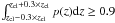 , where zcl is the cluster redshift and p(z) is the photometric redshift probability distribution function output by Eazy (see Sect. 3.1.5).
Stars not identified as such in this phase (12% of our VVDS stars) were removed at a later stage, during the photometric redshift selection and the background statistical subtraction phase.
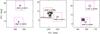 |
Fig. 3 SDSS cluster subsample: spatial location of the seven clusters of our SDSS subsample (red crosses). Magenta/red solid lines represent our SDSS field used for background estimation for each cluster (see Sect. 3.2). For each cluster, blue circles have radii of 0.5 × , 1 × and 2 × r200. Gray areas represent masked regions for fblue estimation and background estimation, due to large-scale structures or potential clusters at similar redshifts as those of our cluster subsample for each field. |
3.1.3. Photometric error correction
We corrected the SExtractor (Bertin & Arnouts 1996) flux errors underestimation caused by the correlation of adjacent pixels during image resampling (e.g. Casertano et al. 2000; Andreon 2001; Raichoor & Andreon 2012) as in Raichoor & Andreon (2012), and found a factor of 1.5, in agreement with previous studies (e.g. Ilbert et al. 2006; Coupon et al. 2009; Raichoor & Andreon 2012).
3.1.4. Photometric calibration
To prevent any systematic offset in colors between fields, which can lead to systematic offsets in the p(z) functions, we matched the color-color diagrams of stars falling in different fields. We selected a reference field (022539-041200), and bright stars (i′ < 21, r2 < 3 pixels, S/N > 20 in all bands, terapix_flag ≤ 1). We adopted a χ2 minimization with 3σ-clipping of stellar sequences in color-color diagrams, holding fixed all parameters but the intercept, which was frozen at the best-fit value of the reference field. This relative photometric calibration (see Table 2) ensures that one measures unbiased p(z) all across our CFHTLS W1 fields.
Photometric correction δ applied to CFHTLS W1 subfields (mnew = mold + δ).
3.1.5. Redshift probability distributions p(z)
To remove galaxies that are very probably in front of or behind the cluster (cf. Sect. 3.1.6), we estimated the full photometric redshift probability distribution function p(z) for each galaxy, using Eazy (Brammer et al. 2008) with default settings and an r-band magnitude prior (see Appendix B). Systematic offsets in the photometric calibration between data and models (e.g., Brodwin et al. 2006; Brammer et al. 2008) were estimated with the same approach as in Raichoor & Andreon (2012): the found offsets are listed in Table 3. These small shifts, comparable with previous works (Ilbert et al. 2006, 2009; Coupon et al. 2009; Barro et al. 2011; Raichoor & Andreon 2012), were applied only during the p(z) estimation.
Systematic offsets mfit − mmeas between measured and best-fit model magnitudes for photometric redshift estimation.
3.1.6. Background removal
We need to account for galaxies along the cluster line of sight, which we generally call background. We again took a conservative approach by only removing galaxies that are very probably in front of or behind the cluster, and by statistically accounting for the residual background in a second step.
First, we performed a photometric redshift selection by removing galaxies that are at z < zcl − 0.05 × (1 + zcl) or z > zcl + 0.05 × (1 + zcl) at ≥ 99% confidence. This selection has been calibrated on our spectroscopic VVDS sample and was accomplished by keeping objects with  (1)
(1)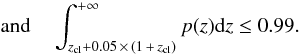 (2)Figure 4 illustrates such a selection criterion for three galaxies.
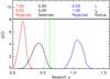 |
Fig. 4 Illustration of the selection criterion applied in Eqs. (1) and (2) with zcl = 0.61: we display p(z) for three galaxies. For each galaxy, we report above the value for I1 (resp. I2), the integral in Eq. (1) (resp. Eq. (2)), and whether the galaxy is selected or not. Vertical green solid and dashed lines represent zcl and zcl ± 0.05 × (1 + zcl), respectively. |
This selection is conservative, because it keeps galaxies in the sample that have a low probability to belong to the cluster. Eqs. (1) and (2) wrongly remove ≲1% of galaxies from our spectroscopic VVDS sample (13/1652). To illustrate the efficiency of this background removal, we display in Fig. 5 the cumulative p(z) function for all objects in the background area for four clusters, before and after applying the selection described by Eqs. (1) and (2). We observe that this selection removes ≳50% of background objects. We note that the same amount of objects are removed for cluster outer regions (1 < r/r200 < 2), but less for cluster core regions (r/r200 < 1), because the background contamination is proportionally lower towards the cluster center.
We thus observe that Eqs. (1) and (2) fulfill our conservative approach criterion: it significantly reduces the sample, with rejecting a non-significant part (≲1%) of the galaxies we are interested in. Changing the {0.05, 0.99} values toward a more stringent selection could reduce the contamination in our sample, but at the cost of removing a more significant part of the galaxies we are interested in. Changing the {0.05, 0.99} values toward a less stringent selection would only increase the contamination in our sample.
 |
Fig. 5 Cumulative p(z) function for all objects in background area for four clusters, before (black curves) and after (magenta curves) applying the selection described by Eqs. (1) and (2). Vertical green solid and dashed lines represent zcl and zcl ± 0.05 × (1 + zcl), respectively. |
As a second stage of the background subtraction, we aimed to select independent control fields taken from the very same data and CFHTLS W1 field as the cluster galaxies, to guarantee homogeneity across the samples. Furthermore, because we aimed to stack data for different clusters, we also needed independent data for the background, so that we did not overstate the quality of the control sample.
We selected for each CFHTLS W1 field a control sample in the same field in the following way. First, we removed objects within 2 × r200 around each cluster and within circles (0.05° radius) around potential clusters at similar redshifts (gray areas in Fig. 2). The several studies on clusters in the CFHTLS W1 fields ensure that contaminating clusters are taken into account. Then, we randomly divided the remaining objects into four subsample to reduce the effect of any potential structure, which assembled four independent control subsamples (each with a surface of ~0.2 deg2). We randomly associated each cluster to a control subsample. When clusters in a common field had similar redshifts (always less than four in our sample), we associated them with different control subsamples in this field, thus never attributing the same background twice.
In addition, this step also subtracts any star that has not been identified as one based on its colors.
3.2. SDSS
SDSS data were analyzed identically. For the SDSS/HIFLUGCS subsample, we worked with data in ugriz bands from the SDSS DR8 (Aihara et al. 2011). We used the ModelMag for galaxy colors, and cModelMag and PsfMag as an approximate total magnitude for galaxies and stars, respectively.
Our SDSS galaxy sample is selected from the Galaxy view of the SDSS DR8, to which we applied a cut in magnitude (cModelMag_r < 19), a spatial cut (10° × 10° around each cluster) and a criterion to reject saturated stars misclassified as galaxies (FiberMag_u ≥ 22−0.5 × ModelMag_u). By matching this catalog with the spectroscopic informations from the main galaxy sample (petroMag_r < 17.8 in SpecPhoto view), we obtained ~30 000 spectroscopic redshifts (zspec ≲ 0.4), which we used to assess the quality of our background removal.
To check that the photometry does not present any systematic offset between our fields, we used more than 10,000 spectroscopic stars from the SpecPhoto view located in our fields in in the same way as for the CFHTLS W1 fields (Sect. 3.1.4). We found indeed no offset greater than 0.01 mag for all filters and all fields.
We estimated the p(z) in in the same way as for the CFHTLS W1 fields (Sect. 3.1.5). We applied the photometric offsets listed in Table 3.
For background removal, we selected galaxies as in Sect. 3.1.6. This criterion removes ~20% of the background objects, and wrongly removes ~0.05% of the spectroscopic objects. For each cluster, we selected as a control sample objects within a 10° × 10° area around each cluster, excluding objects within 2 × r200 around each cluster and within circles (0.3° radius) around potential clusters at similar redshifts. For clusters A2052 and A2063, we defined two independent control subsamples as described in Sect. 3.1.6 and using the region within the red solid line in Fig. 3. The resulting control samples are ~90 deg2 (resp. ~50 deg2) for the MKW4, A1367, MKW8, A2634, and A2657 clusters (resp. the A2052 and A2063 clusters).
3.3. Settings for the estimation of fblue
We describe in this section our procedure for consistently measuring the fraction of blue galaxies fblue. The procedure described here is similar to the one followed in Sect. 4 of Raichoor & Andreon (2012) for JKCS 041.
For each cluster, we considered three radial bins (annuli) at distinct cluster-centric radii, defined by r/r200 ≤ 0.5, 0.5 < r/r200 ≤ 1, and 1 < r/r200 ≤ 2.
3.3.1. Probed color
To probe the same rest-frame color at all redshifts as consistently as possible, we worked in a color-magnitude diagram that closest corresponds to the (u − r) vs. r rest-frame, thus probing the 4000 Å break. Figure 6 illustrates the filters chosen at each redshift of our sample. Because our reddest band for the CFHTLS W1 sample is the z band, this implies a drift in the probed rest-frame red band when the redshift is approaching 1 (z = 0.77 and z = 1.05): we are here limited by the data, but still improve on previous works (see for instance Loh et al. 2008).
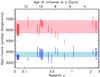 |
Fig. 6 (u − r)-like rest-frame probed color: for each cluster of our sample, we plot the rest-frame probed color as a function of the redshift. The shaded areas indicate the wavelength intervals where the filter response convolved with a typical elliptical galaxy spectrum is above half of its maximum value. The vertical bars represent the same for the redshifts of our clusters and the corresponding chosen filters. |
The top panel of Fig. 7 illustrates another possible choice of filter pairs, matching the (B − V) rest-frame color. The bottom panel shows that fblue – estimated as described below – does not depend on the precise sampling of the filters, given that they bracket the 4000 Å break. Our results are robust regarding the rest-frame color: using the (B − V) color instead of (u − r) leads to similar values of fblue (see Fig. 7).
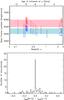 |
Fig. 7 Dependence of fblue on the rest-frame probed color. Top: like Fig. 6, but for B − V rest-frame color. Bottom: we compare the estimated fblue when using the rest-frame B − V and u − r colors for 84 estimated values (10 clusters for which are available independent filter pairs probing the rest-frame B − V and u − r colors, 1 to 4 mass bins, 3 radial bins). We stress that some individual estimates of fblue have large error bars (see Fig. 10): the 68% shortest intervals for fblue(B − V) and fblue(u − r) all intersect. |
3.3.2. Mass bin defintion
For our values of mass M we refer, as in previous works, to the Bruzual & Charlot (2003) model (2007 version, CB07 hereafter) mass, and specifically to the mass of the gas that will eventually be turned into stars, i.e. the integral of the star formation rate (Andreon et al. 2008; Raichoor & Andreon 2012). This mass definition has the advantage to compare galaxies at each epoch that will end up with the same stellar mass, which means that we include in each mass bin the same galaxies at high and low redshifts. In the color–magnitude diagrams, the shape of these loci of constant mass differ from that which corresponds to the mass in stars at the redshift of observation (Mzobs) on the blue end (see Fig. 8): the higher the redshift, the more fainter/bluer objects are included in our definition. For instance, a galaxy with an exponentially declining SFH ∝ exp [−(t/τ)] with τ = 3 Gyr would have a mass in stars of ~30/50/90% of its final mass in stars after ~ 0.8/1.6/5.3 Gyr: had we chosen the mass in stars at redshift of observation as a definition of stellar mass, such a galaxy would not be included in our sample at high redshift, then would enter it at a given epoch and drift from one mass bin to another at an irregular pace, thus biasing the result. We discuss in Sect. 5.2 the impact of this definition on our results.
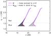 |
Fig. 8 Illustration of a mass bin definition (zobs = 0.49, 10.73 ≤ log (M/M⊙) < 11.13): thick magenta solid lines represent the loci of constant mass M used in this study (the mass evolved to z = 0), thick blue dashed lines the loci of constant mass Mzobs in stars at zobs, and gray shaded areas represent the difference between those two definitions. The horizontal dotted line represents the threshold used to define blue/red galaxies. |
We used four galaxy mass bins (log (M/M⊙) in [9.92, 10.33[, [10.33, 10.73[, [10.73, 11.13[, and [11.13, +∞[). We hereafter refer to those galaxy mass bins by using the mean value of each bin (using a Schechter 1976 function), i.e. ⟨ log (M/M⊙) ⟩ ~ 10.14, 10.54, 10.94, and 11.47. These (model) masses are computed for solar metallicity, a formation redshift of zform = 5 (setting zform to 4 or 6 does not change our results), and either SSP or an exponentially declining star-forming τ model with 0 < SFH τ (Gyr) ≤ 10. The mass values used to define mass bins correspond to the mass of an SSP model having at z = 0 a V-band absolute rest-frame magnitude MV of –17.8, –18.8, –19.8, and –20.8.
The depth of the data limits the sampled mass range: for each cluster, we required that the lowest mass cut is brighter than a signal-to-noise ratio of 5 in the considered color-magnitude diagram. This constraint – probing higher masses at higher redshifts – restricts the mass range probed, but ensures that we work on mass-complete samples and allows a direct comparison of fblue values at different redshift and mass bins.
3.3.3. Blue/red definition
We define a galaxy as blue if it is bluer than a CB07 model with τ = 3.7 Gyr, as in Andreon et al. (2004, 2006, 2008), Loh et al. (2008), and Raichoor & Andreon (2012). This galaxy will be bluer by 0.2 mag in B − V than red-sequence galaxies at z = 0 (which would be a blue galaxy by the original definition of Butcher & Oemler 1984). As a comparison, our definition agrees at z = 0 with that used in Peng et al. (2010), and efficiently splits the red-sequence and the blue cloud of their SDSS data. The rationale behind our choice is to take into account the stellar evolution of galaxies with time. Figure 9 illustrates the rest-frame u − r color evolution for different exponentially declining τ-SFHs: the different tracks do not cross each other. In other words, if a galaxy follows an exponentially τ-SFH with τ < 3.7 Gyr (resp. τ > 3.7 Gyr) during its lifetime, its color according to our definition will remain red (resp. blue). However, we note that this figure assumes that all galaxies have the same zform. We will return to this point in Sect. 5.
In addition, we stress that the independence of fblue on the probed rest-frame color (Sect. 3.3.1) is a consequence of our choice to define red and blue galaxies (see Fairley et al. 2002 for an opposite result when using the red-sequence to split red and blue galaxies).
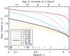 |
Fig. 9 Model rest-frame u − r color evolution for different exponentially declining τ-SFHs (CB07 models, solar metallicity and zform = 5). According to our definition a galaxy is classified as red (resp. blue) if it is redder (resp. bluer) than a model with τ = 3.7 Gyr. The vertical arrows indicate the redshifts of our cluster sample. |
4. Results
We present in this section the dependence of fblue with galaxy mass, cluster-centric distance and redshift. We recall that the evolution of fblue with redshift traces the fraction of cluster galaxies that have stopped forming stars, under the assumption of an average exponentially declining star formation history for cluster galaxies. Indeed, under our working assumptions and our definition of blue/red galaxies, any quenching implies a lowering of fblue with redshift, whereas no quenching implies an fblue constant with redshift. Hence our results present the evolution with redshift of the star formation activity in clusters as a function of galaxy mass and environment.
Before performing a general analysis, we start by a simple analysis that makes partial use of the data (Sect. 4.1) and that therefore does not show trends in a similar clear way (Sects. 4.2 and 4.3). Our main result is presented in Sect. 4.3 and illustrated in Fig. 13: environmental and mass quenching are separable, environmental quenching does not change with epoch, and mass quenching is a dynamical process, i.e. its evolutionary rate is mass-dependent.
4.1. Results for individual clusters
For each cluster, galaxy mass bin, and radial area we computed the blue fraction fblue that accounts for residual background galaxies (i.e. along the line of sight, kept by the criteria of Eqs. (1) and (2), and not belonging to the cluster) using our control samples (as defined in Sect. 3.1.6) and following the Bayesian methods introduced in Andreon et al. (2006). We adopt uniform priors for the parameters.
Figure 10 displays the individual fblue profiles for our cluster sample, grouped by redshift and mass bins. We defined our redshift bins so that each bin spans a period of ~ 2 Gyr (0 ≤ z < 0.16, 0.16 ≤ z < 0.37, 0.37 ≤ z < 0.65, 0.65 ≤ z < 1.1, and z ~ 2.2). We hereafter refer to those redshift bins by using the median value of our cluster sample in each bin, i.e. ⟨ z ⟩ ~ 0.03, 0.31, 0.49, 1.05, and 2.2. We can already observe some indications of the trends that we later perceive in stacking analysis.
We observe a different behavior for different galaxy mass bins: at ⟨ z ⟩ ~ 0.31, fblue(r/r200 ≤ 0.5) decreases (from ~0.4 to ~0) with increasing galaxy mass. fblue seems to increase with increasing r/r200: for instance, at ⟨ z ⟩ ~ 0.03 for the less massive galaxies, fblue increases with increasing cluster-centric distance. For the most massive galaxies, fblue(r/r200 ≤ 0.5) ~ 0 at all redshifts.
However, the unavoidable noise – because of the finite and usually small number of member galaxies per cluster at a given mass and cluster-centric distance bins – makes it difficult to draw a general picture.
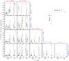 |
Fig. 10 fblue for individual clusters as a function of cluster-centric distance (r/r200) for different bins of redshift (increasing rightward) and galaxy mass (increasing downward). The computed value of fblue already takes into account the mean aging of stars with increasing redshift by defining the color compared to an exponentially declining SFH model with τ = 3.7 Gyr. Error bars represent the shortest interval including 68% of the possible posterior values for fblue, and are plotted as a dashed line when this interval is larger than 0.66, indicating that fblue is not constrained at all. Radial cluster-centric bins are indicated by gray filled triangles on the x-axis and horizontal gray dashed lines indicate the minimum and maximum allowed values for fblue. |
4.2. Results for stacked clusters
We now stacked our sample according to redshift and mass bins to strengthen the estimated fblue. For each panel of Fig. 10, we computed the mean fblue for all clusters belonging to this panel, multiplying the individual data likelihoods, and then using the Bayes theorem as in the previous section. We recall that the combined data are independent, in particular the control samples. The values of fblue are reported in Table 4 and displayed in Fig. 11 as dots with error bars. Now the trends are emerging quite clearly.
Regarding the dependence of fblue with cluster-centric distance, our data seem to indicate an increase in fblue with increasing r/r200, for most redshift and mass bins. The cluster color profile at given galaxy mass tends to flatten with decreasing redshift. In particular, the flat profile is achieved at the lowest redshift and most massive galaxies. For all mass and radial bins, our data suggest a decrease of fblue with decreasing redshift. For our two lowest mass bins, this evolutionary trend is strong. For the highest mass bin, this decrease is marginal, because fblue already has very low values at high redshifts.
Finally, we also see a trend when looking at the dependence of fblue with galaxy mass. Indeed, for our two lowest redshift bins, where our data span four mass bins, we observe a clear trend at all radial bins: at fixed redshift and cluster-centric distance, fblue decreases with increasing galaxy mass. For instance, for the innermost radial bin and ⟨ z ⟩ ~ 0.03, fblue decreases continuously (with increasing galaxy mass) from  to
to  . For ⟨ z ⟩ ~ 0.49, though our data only span two mass bins, we observe the same trend. Our analysis shows that there is – in addition to the known mean aging of the stellar populations – a decrease at all radii in fblue with decreasing redshift, the intensity of which decreases when the galaxy mass increases, and disappears for the most massive galaxies.
We note that in one panel of Fig. 11 ( ⟨ z ⟩ ~ 0.31 and ⟨ log (M/M⊙) ⟩ ~ 11.47), our data present an odd behavior for r/r200 ≥ 1: the value of fblue is quite high and does not reflect the general trend, as the mismatch with the fit (detailed below) illustrates. However, we keep in mind that the 0 value is just at 2σ.
fblue for our cluster sample stacked by redshift and galaxy mass bins.
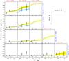 |
Fig. 11 fblue for stacked clusters as a function of cluster-centric distance (r/r200) for different bins of redshift (increasing rightward) and galaxy mass (increasing downward). The computed value of fblue already takes into account the mean aging of stars with increasing redshift by defining the color compared to an exponentially declining SFH model with τ = 3.7 Gyr. Error bars represent the shortest interval including 68% of the possible posterior values for fblue. Radial cluster-centric bins are indicated by gray filled triangles on the x-axis and horizontal gray dashed lines indicate the minimum and maximum allowed values for fblue. Yellow shaded areas with a solid blue line represent the posterior mean and 68% confidence interval of the modeling of Eq. (3), fitting the 225 individual fblue measurements. Yellow slanting hatched areas with a dashed blue line represent the prediction/extrapolation of this model for bins where we do not have data. Cyan vertically hatched areas with solid magenta line (in two panels only) illustrate how the model fit fails if the ζ term in Eq. (3) is not included. |
4.3. Results for the whole sample
We now fitted the 225 values of fblue (26 clusters, 3 radial bins, 1 to 4 galaxy mass bins) at once by modeling at the same time the dependence of fblue on galaxy mass M, redshift z and cluster-centric distance r/r200. In this section, we are no longer ignoring redshift differences inside each panel, and the collective use of the whole dataset allows us to strengthen the trends even more.
As detailed below, to describe the data, we also need an interaction term between galaxy mass and redshift, a term that allows galaxies of different mass to evolve at different rates. We use the following model: ![Mathematical equation: \begin{eqnarray} {f_{\rm blue}} \left(r/r_{200},M,z \right) &=& \texttt{ilogit} \, \Bigl[ A_0 \nonumber\\ && +\,\alpha \ \log \left(r/(0.25 \cdot r_{200}) \right) \nonumber \\ && +\,\beta \ (\log(M/M_{\odot}) - 11) \nonumber\\ && +\,\gamma \ (z-0.3) \nonumber \\ && +\,\zeta \ (\log(M/M_{\odot})-11) \ (z-0.3) \Bigr], \label{eq:model} \end{eqnarray}](/articles/aa/full_html/2012/07/aa19091-12/aa19091-12-eq198.png) (3)where ilogit(x) = (1 + exp( − x))-1 ensures that 0 ≤ fblue ≤ 1. We adopt uniform priors for the parameters A0, α, β, γ, and ζ.
(3)where ilogit(x) = (1 + exp( − x))-1 ensures that 0 ≤ fblue ≤ 1. We adopt uniform priors for the parameters A0, α, β, γ, and ζ.
The model fit results are plotted in Fig. 11 as solid blue lines and yellow shaded areas (68% confidence interval), while the model prediction/extrapolation is plotted as dashed blue lines and yellows hatched areas.
The only motivation behind the chosen parametrization is the adoption of an additive model that fits our data and ensures that 0 ≤ fblue ≤ 1. The adopted model is the simplest one fulfilling those criteria. If we do not include the ζ term, the model cannot fit data in the redshift bins ⟨ z ⟩ ~ 0.31 for galaxies within our two lowest mass bins (see cyan vertically hatched areas in Fig. 11) and, to a lesser extent, in the panel ⟨ z ⟩ ~ 0.49 and ⟨ log (M/M⊙) ⟩ ~ 10.94. In a similar manner, if we replace the term crossing M and z by a term crossing r and z or r and M, the model fails in fitting the data. Furthermore, we note that adding a term crossing r and z (in addition to our ζ term) does not improve the quality of the fit. The fblue evolution with redshift is therefore more sensitive to the galaxy mass than to its cluster-centric distance.
The posterior probabilities for the model parameters are plotted in Fig. 12, which shows how our knowledge about the parameters changes from before (prior, blue line) to after (posterior, black/red lines) the data. In short, the posterior distribution of all parameters is much more concentrated than the prior, i.e. data are highly informative about these parameters and conclusions on these parameters do not depend on the adopted prior.
The values agree with our qualitative trends put forth in Sect. 4.2, with fblue increasing with cluster-centric distance ( ), decreasing with galaxy mass (
 ), and increasing with redshift (
 ). ζ measures the relative speed – when compared to the evolution of galaxies with log (M/M⊙) = 11 – at which fblue evolves as a function of galaxy mass. Because ζ is negative (
 ), galaxies with lower masses will on average evolve on longer timescales. We note that our model is constrained at z ≫ 1 only by the JKCS 041 cluster (if we repeat the fit without the JKCS 041 data, the model appears to be entirely unconstrained in the ⟨ log (M/M⊙) ⟩ ~ 11.47 and z ~ 2.2 window).
To better visualize the dependence of fblue on those three parameters (M, r/r200, and z), we display in Fig. 13 the variations of fblue on two of them when fixing the third one. The information (data and model fit/predictions) is exactly the same as in Fig. 11, only presented differently. We recall that our model is only constrained where there are some data (shaded areas), and that the fit was performed on the individual 225 values of fblue. This figure illustrates on the one hand that at fixed cluster-centric distance, fblue evolves at different paces for different galaxy stellar masses (panels a and b), captured by the ζ term in our model. On the other hand, we can see in panel c that the model evolution of fblue with z at fixed galaxy mass has a similar shape for our values of r/r200. Lastly, panel d summarizes the radial profiles of fblue at a fixed redshift for different galaxy mass bins.
4.4. Results for the original Butcher and Oemler cut
Adopting a mass threshold corresponding to the original Butcher & Oemler (1984) one (log (M/M⊙) ≥ 10.53), we observe no evolution of fblue with redshift for our data (z ≤ 0.43) (see Fig. 14). However, when extrapolating the model to z = 1.05, we observe an increase in fblue, in broad agreement with the measurement done by Andreon et al. (2008) for the RzCS 052 cluster.
That almost no evolution is found at z ≤ 0.43, whereas we do detect one for ⟨ log (M/M⊙) ⟩ ~ 10.54, nicely illustrates the benefit of splitting our sample into fine galaxy mass bins.
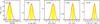 |
Fig. 12 For each parameter fitted with the model of Eq. (3), we plot as a black lines the posterior probability function and as yellow shaded area the shortest interval including 68% of the possible posterior values. We report the point estimate and the 68% confidence interval on each panel, and overplot as a thick red line the corresponding Gaussian curve. The blue lines represent the uniform prior used for the fit. |
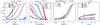 |
Fig. 13 Dependence of fblue on M and z at fixed r/r200 (panels a and b), on z and r/r200 at fixed M (panel c), and on M and r/r200 at fixed z (panel d). Data points with error bars are the same as in Fig. 11. Shaded areas represent the posterior mean and 68% confidence interval of the modeling of Eq. (3), fitting the 225 individual fblue measurements. Prediction/extrapolation of this model for bins where we do not have data are plotted as hatched areas and dashed lines. X-axis bins are indicated by gray filled triangles on the x-axis and horizontal gray dashed lines indicate the minimum and maximum allowed values for fblue. |
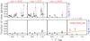 |
Fig. 14 Evolution of fblue for individual (top panels) and stacked (bottom panels) clusters as a function of cluster-centric distance (r/r200) for different bins of redshift (increasing rightward) for a mass-selected sample with a mass corresponding to the original MV in Butcher & Oemler (1984). Symbols are as in Figs. 10 and 11. We add a new panel at z = 1.05 for model prediction, where we overplot the measured values of fblue for the RzCS 052 cluster in Andreon et al. (2008). |
5. Discussion and conclusion
Our aim was to put constraints on the different processes responsible for the cessation of star formation activity (“quenching”) in clusters through a careful study of the dependence of the fraction of blue galaxies fblue in clusters that span a broad redshift baseline. We have built a cluster sample consisting of seven clusters (0.02 ≤ zspec ≤ 0.04) from the HIFLUGCS survey, eighteen clusters (0.14 ≤ zspec ≤ 1.05) from the XMMLSS survey, and JKCS 041 (z ~ 2.2). Because the HIFLUGCS and XMMLSS surveys are X-ray selected, our cluster sample is unbiased regarding the fraction of blue galaxies fblue at a given cluster mass; in addition, our clusters were chosen to have similar masses. For different galaxy mass and cluster-centric distance bins, we carefully estimated fblue for each cluster and fitted the dependence of fblue with redshift, galaxy mass and cluster-centric distance. We did not attempt to invert the noisy data because of the degeneracy between zform, age (and metallicity), but instead we modified the model until it fitted the data. The reference model has an exponentially declinining SFH, and hence an evolving mass (if stars are formed, mass in stars cannot be fixed). Deviations from this reference model highlight the evolution and respective role of the quenching in clusters due to galaxy mass or to environment.
Our main result is displayed in Figs. 11 and 13. We recall that in those figures we have already taken into account that galaxies are on average younger at higher redshifts, by using an exponentially declining τ-model to define whether a galaxy is red or blue. This means that any measured evolution of fblue with redshift reflects a phenomenon in addition to the younger mean age of the Universe and the secular increase in the star formation rate. We also recall that our model fitting was performed on the 225 individual measurements of fblue. Moreover, our definition of galaxy mass ensures that, for each mass bin, the selected high-redshift galaxies are those that would end up in the low-redshift galaxies selection.
We are therefore able to disentangle for the first time the role of secular evolution, galaxy mass and cluster-centric distance on galaxy evolution in clusters. We found that fblue decreases with decreasing redshift z, with decreasing cluster-centric distance r/r200, and with increasing galaxy mass M. This means that the processes responsible for the cessation of star formation in clusters are effective at all epochs (z ≲ 2.2) and more effective in denser environments and for more massive galaxies. Our (simple) modeling of the data shows that the dependence of fblue on galaxy mass evolves with redshift, while this is not the case for the dependence of fblue on cluster-centric distance: the intensity of mass quenching evolves with redshift at different paces for different galaxy masses, whereas the environmental quenching does not evolve with redshift. Additionally, our data did not need any correlation between galaxy mass and cluster-centric distance in the model fitting, which means that mass quenching and environmental quenching are separable.
5.1. Remark on taking into account secular evolution when estimating fblue
We illustrate in this section the advantage of taking into account secular evolution when estimating fblue: using a non-evolving color threshold (e.g. Presotto et al. 2012) will result in using a redder color to split blue and red galaxies, hence in increasing fblue.
As a test, we repeated our analysis, with a non-evolving, mass-dependent definition of blue/red galaxy. For low redshifts (z ≲ 0.5), this leads to results marginally different from ours, because the colors used in the two methods to split blue and red galaxies do not differ significantly. However, for higher redshifts, we do observe a notable difference between the two methods, because the difference between the two definitions of blue/red galaxies will increase with increasing redshift. For instance, using a non-evolving color threshold leads to larger blue fractions at z ≳ 1 (0.2 ≲ fblue ≲ 0.6) for stacked data. Since fblue depends on r/r200, a non-evolving color threshold also tilts the fblue profile. Overall, the results using a non-evolving color threshold are much harder to interpret, because there is an additional effect that depends on the redshift (and potentially the radial) bin(s) under inspection.
5.2. Remark on using evolved mass definition
We remark that using the mass in stars at the redshift of observation, Mzobs, as a mass definition does not appreciably change our conclusions: the estimated values of fblue are slightly lower, but the trivariate dependence of fblue on redshift, galaxy mass and cluster-centric distance remains similar (the α, β, γ, and δ parameters vary by less than 1σ).
Indeed, as illustrated in Fig. 8, lines of constant mass at the redshift of observation in the color − magnitude diagrams are similar to those used in the study, but for blue colors. For a considered mass bin, using Mzobs instead of M will remove galaxies in the light-gray shaded area, but add those in the dark-gray shaded area. Because of the mass function shape, the former will on average be slightly more numerous than the latter: the net effect will be to slightly decrease the number of blue galaxies, hence fblue.
5.3. Dependence of fblue on M and z
The data and their fit point out two results:
-
The average SFH is more complex than exponentially decliningSFHs, as quantified by the γ and ζ terms. Indeed, if cluster galaxieshad on average exponentially declining SFHs, we should notobserve any change of the fblue radial profile with redshift (at fixedgalaxy mass). Low-mass galaxies may have a briefly enhancedSFH because of starbust, hence temporarily a color bluer than anSFH τ = 3.7 Gyr model, after which their color turns red-der than an SFH τ = 3.7 Gyr model. For our lowest massbin, this mechanism would still be at work at z < 0.37. We also consideredthe case of a later zform for low-mass galaxies. We experimented withsome possible choices without being able to remove the observedevolution of fblue with redshift, although our tests are not exhaustiveand we are reaching the limit of the data.
-
There is a differential evolution of fblue with the galaxy mass, i.e. mass quenching is a dynamical process. Galaxies with smaller masses evolve later: for instance, at z ≤ 0.37, fblue for galaxies in our lowest mass bin still evolve significantly, which is not the case for fblue for more massive galaxies.
Furthermore, less massive galaxies seem to evolve on a longer timescale than more massive galaxies. In the ~3 Gyr between our two lowest redshift bins, fblue changes by ~0.4 for low-mass galaxies. In less time (~2 Gyr), fblue should change by twice as much at z ≳ 2 for high-mass galaxies.
5.4. Dependence of fblue on r/r200
We now turn to the analysis of the dependence of fblue with cluster-centric distance r/r200. For all galaxy stellar mass and redshift bins, fblue decreases with decreasing r/r200, i.e. environmental quenching is effective at all redshifts and stellar masses (Fig. 11). This effect is conspicuous on lower mass galaxies, as fblue is very low for massive galaxies, whatever the cluster-centric distance (one should observe a significant number of clusters at z ~ 1–2 to see this effect on massive galaxies). Previous works clearly established this dependence on r/r200 for mass-selected samples (e.g. Andreon et al. 2008; Haines et al. 2009), however, our study shows for the first time that this dependence holds for different galaxy mass bins. In addition, the model fitting our data implies that the mass and environmental quenchings are fully separable, because no crossed term between M and r/r200 is required.
Additionally, we found that our data do not require any evolution of this dependence with redshift: our (simple) model requires only a crossed term between M and z, none between r/r200 and z. This can be interpreted that either this evolution with z of the environmental quenching is not present, or that is of second order when compared to the evolution with z of the mass quenching. We recall that our cluster sample consists of clusters having similar temperatures at all redshifts, while a self-similarly evolving cluster model (Kaiser 1986) suggests a mild increase with redshift at 0 < z < 1. Nevertheless, current studies tend to show that fblue estimated in the virial radius is independent of cluster mass, at least in the local Universe (e.g., De Propris et al. 2004; Goto 2005).
Finally, we would like to emphasize the importance of the backsplash population on the fblue radial profile and its evolution with redshift: galaxies as far away as two virial radii may have been within the main body of the cluster in the past (e.g., Balogh et al. 2000; Gill et al. 2005; Mahajan et al. 2011).
5.5. Conclusion
Our study extends the relationship between galaxy mass, star formation rate and environment at z ≲ 1 explored by Peng et al. (2010) to intermediate-mass cluster environments. As those authors, we found that the cessation of star formation (“quenching”) due to environment and galaxy mass are separable (we needed no crossed term between r/r200 and M to fit our data), that environmental quenching does not change with epoch (we needed no crossed term between r/r200 and z to fit our data), and that mass quenching is a dynamical process (we did need a crossed term between M and z to fit our data). The close agreement between the two studies is likely a consequence of the common choices adopted for the two analyses: disentangling galaxy mass and environment, plus taking into account the secular aging of stars with decreasing redshift, as described by Andreon et al. (2006). However, in addition to paying special attention to the statistical aspect of the analysis (which allowed us to provide good confidence intervals on our measurements), our study implemented a finer control on galaxy mass (by considering the mass evolved at z = 0) and on environmental estimation (using r/r200 is less subject to biases than a density field based on rest-frame B-band selection).
Muzzin et al. (2012), investigating a cluster sample at z ~ 1 with spectroscopic data, made a similar analysis, studying the role of galaxy mass and environment (but not secular evolution) on star formation. The availability of spectroscopic data allows estimating the star formation rate, and thus a thorough analysis of this problem. Regarding the fraction of star-forming galaxies, these authors also concluded that mass and environmental quenching are separable. Our work extends this study by including the redshift dependence in the analysis, by a better characterization (r200) of cluster properties, and by using a cluster sample that is not selected by a galaxy property under study (color).
Our study extends the downsizing-like scenario to cluster environment and all galaxies, which was already established for galaxies with specific properties in the field (e.g., emission line: Cowie et al. 1996; spheroidal: Treu et al. 2005; passive: Peng et al. 2010). According to this scenario, the properties of the most massive galaxies are established in the very early Universe (z ≫ 1), while less massive galaxies continue to evolve at redshifts 0 < z < 1. We stress that our downsizing-like scenario concerns all galaxies, regardless of their morphology or color. The results of Andreon et al. (2008) and Raichoor & Andreon (2012) taken as a whole point to a similar conclusion, though for smaller cluster samples.
Our work is the first to study the dependence of fblue in clusters on galaxy mass, redshift, and cluster-centric distance at the same time, with a cluster sample whose properties are well-controlled. In particular, it clearly demonstrates the need to use galaxy mass as a parameter to better understand the behavior of fblue. This approach is now possible with the wealth of available data.
Acknowledgments
We thank the anonymous referee for his/her careful reading and suggestions, which improved the clarity of the paper. We acknowledge financial contribution from the agreement ASI-INAF I/009/10/0 and from Osservatorio Astronomico di Brera. Based on data from SDSS-III (full text acknowledgement is at http://www.sdss3.org/collaboration/boiler-plate.php) and observations obtained with MegaPrime/MegaCam (http://www.cfht.hawaii.edu/Science/CFHLS/cfhtlspublitext.html) and WIRCAM (http://ftp.cfht.hawaii.edu/Instruments/Imaging/WIRCam/WIRCamAcknowledgment.html) at CFHT.
References
- Aihara, H., Allen de Prieto, C., An, D., et al. 2011, ApJS, 193, 29 [NASA ADS] [CrossRef] [Google Scholar]
- Andreon, S. 2001, ApJ, 547, 623 [NASA ADS] [CrossRef] [Google Scholar]
- Andreon, S., & Ettori, S. 1999, ApJ, 516, 647 [NASA ADS] [CrossRef] [Google Scholar]
- Andreon, S., & Huertas-Company, M. 2011, A&A, 526, A11 [NASA ADS] [CrossRef] [EDP Sciences] [Google Scholar]
- Andreon, S., Lobo, C., & Iovino, A. 2004, MNRAS, 349, 889 [NASA ADS] [CrossRef] [Google Scholar]
- Andreon, S., Quintana, H., Tajer, M., Galaz, G., & Surdej, J. 2006, MNRAS, 365, 915 [NASA ADS] [CrossRef] [Google Scholar]
- Andreon, S., Puddu, E., de Propris, R., & Cuillandre, J. 2008, MNRAS, 385, 979 [NASA ADS] [CrossRef] [Google Scholar]
- Andreon, S., Maughan, B., Trinchieri, G., & Kurk, J. 2009, A&A, 507, 147 [NASA ADS] [CrossRef] [EDP Sciences] [Google Scholar]
- Andreon, S., Trinchieri, G., & Pizzolato, F. 2011, MNRAS, 412, 2391 [NASA ADS] [CrossRef] [Google Scholar]
- Baldry, I. K., Balogh, M. L., Bower, R. G., et al. 2006, MNRAS, 373, 469 [NASA ADS] [CrossRef] [Google Scholar]
- Balogh, M. L., Navarro, J. F., & Morris, S. L. 2000, ApJ, 540, 113 [NASA ADS] [CrossRef] [Google Scholar]
- Barro, G., Pérez-González, P. G., Gallego, J., et al. 2011, ApJS, 193, 30 [NASA ADS] [CrossRef] [Google Scholar]
- Bertin, E., & Arnouts, S. 1996, A&AS, 117, 393 [NASA ADS] [CrossRef] [EDP Sciences] [Google Scholar]
- Blanton, M. R., Hogg, D. W., Bahcall, N. A., et al. 2003, ApJ, 594, 186 [NASA ADS] [CrossRef] [Google Scholar]
- Brammer, G. B., van Dokkum, P. G., & Coppi, P. 2008, ApJ, 686, 1503 [NASA ADS] [CrossRef] [Google Scholar]
- Brodwin, M., Brown, M. J. I., Ashby, M. L. N., et al. 2006, ApJ, 651, 791 [NASA ADS] [CrossRef] [Google Scholar]
- Bruzual, G., & Charlot, S. 2003, MNRAS, 344, 1000 [NASA ADS] [CrossRef] [Google Scholar]
- Butcher, H., & Oemler, Jr. A., 1978, ApJ, 226, 559 [NASA ADS] [CrossRef] [Google Scholar]
- Butcher, H., & Oemler, Jr., A. 1984, ApJ, 285, 426 [NASA ADS] [CrossRef] [Google Scholar]
- Carlberg, R. G., Yee, H. K. C., Ellingson, E., et al. 1997, ApJ, 485, L13 [NASA ADS] [CrossRef] [Google Scholar]
- Casertano, S., de Mello, D., Dickinson, M., et al. 2000, AJ, 120, 2747 [NASA ADS] [CrossRef] [Google Scholar]
- Chabrier, G. 2003, PASP, 115, 763 [NASA ADS] [CrossRef] [Google Scholar]
- Coupon, J., Ilbert, O., Kilbinger, M., et al. 2009, A&A, 500, 981 [NASA ADS] [CrossRef] [EDP Sciences] [Google Scholar]
- Cowie, L. L., Songaila, A., Hu, E. M., & Cohen, J. G. 1996, AJ, 112, 839 [Google Scholar]
- De Propris, R., Stanford, S. A., Eisenhardt, P. R., & Dickinson, M. 2003, ApJ, 598, 20 [NASA ADS] [CrossRef] [Google Scholar]
- De Propris, R., Colless, M., Peacock, J. A., et al. 2004, MNRAS, 351, 125 [NASA ADS] [CrossRef] [Google Scholar]
- Dressler, A. 1980, ApJ, 236, 351 [NASA ADS] [CrossRef] [Google Scholar]
- Dressler, A., Oemler, Jr., A., Couch, W. J., et al. 1997, ApJ, 490, 577 [NASA ADS] [CrossRef] [Google Scholar]
- Fairley, B. W., Jones, L. R., Wake, D. A., et al. 2002, MNRAS, 330, 755 [NASA ADS] [CrossRef] [Google Scholar]
- Finoguenov, A., Reiprich, T. H., & Böhringer, H. 2001, A&A, 368, 749 [NASA ADS] [CrossRef] [EDP Sciences] [Google Scholar]
- Gill, S. P. D., Knebe, A., & Gibson, B. K. 2005, MNRAS, 356, 1327 [NASA ADS] [CrossRef] [Google Scholar]
- Goto, T. 2005, MNRAS, 356, L6 [NASA ADS] [CrossRef] [Google Scholar]
- Haines, C. P., Smith, G. P., Egami, E., et al. 2009, ApJ, 704, 126 [NASA ADS] [CrossRef] [Google Scholar]
- Hansen, S. M., Sheldon, E. S., Wechsler, R. H., & Koester, B. P. 2009, ApJ, 699, 1333 [NASA ADS] [CrossRef] [Google Scholar]
- Hogg, D. W., Blanton, M. R., Eisenstein, D. J., et al. 2003, ApJ, 585, L5 [NASA ADS] [CrossRef] [Google Scholar]
- Hudson, D. S., Mittal, R., Reiprich, T. H., et al. 2010, A&A, 513, A37 [NASA ADS] [CrossRef] [EDP Sciences] [Google Scholar]
- Ilbert, O., Arnouts, S., McCracken, H. J., et al. 2006, A&A, 457, 841 [NASA ADS] [CrossRef] [EDP Sciences] [Google Scholar]
- Ilbert, O., Capak, P., Salvato, M., et al. 2009, ApJ, 690, 1236 [NASA ADS] [CrossRef] [Google Scholar]
- Kaiser, N. 1986, MNRAS, 222, 323 [NASA ADS] [CrossRef] [Google Scholar]
- Kauffmann, G., White, S. D. M., Heckman, T. M., et al. 2004, MNRAS, 353, 713 [NASA ADS] [CrossRef] [Google Scholar]
- Kron, R. G. 1995, Evolution in the Galaxy Population, ed. A. R. Sandage, R. G. Kron, M. S. Longair, B. Binggeli, & R. Buser, 233 [Google Scholar]
- Le Fèvre, O., Vettolani, G., Garilli, B., et al. 2005, A&A, 439, 845 [NASA ADS] [CrossRef] [EDP Sciences] [Google Scholar]
- Lilly, S. J., Le Fevre, O., Hammer, F., & Crampton, D. 1996, ApJ, 460, L1 [NASA ADS] [CrossRef] [Google Scholar]
- Loh, Y.-S., Ellingson, E., Yee, H. K. C., et al. 2008, ApJ, 680, 214 [NASA ADS] [CrossRef] [Google Scholar]
- Madau, P., Pozzetti, L., & Dickinson, M. 1998, ApJ, 498, 106 [NASA ADS] [CrossRef] [Google Scholar]
- Mahajan, S., Mamon, G. A., & Raychaudhury, S. 2011, MNRAS, 416, 2882 [NASA ADS] [CrossRef] [Google Scholar]
- Margoniner, V. E., de Carvalho, R. R., Gal, R. R., & Djorgovski, S. G. 2001, ApJ, 548, L143 [NASA ADS] [CrossRef] [Google Scholar]
- Muzzin, A., Yee, H. K. C., Hall, P. B., & Lin, H. 2007, ApJ, 663, 150 [NASA ADS] [CrossRef] [Google Scholar]
- Muzzin, A., Wilson, G., Yee, H. K. C., et al. 2012, ApJ, 746, 188 [NASA ADS] [CrossRef] [Google Scholar]
- Navarro, J. F., Frenk, C. S., & White, S. D. M. 1997, ApJ, 490, 493 [NASA ADS] [CrossRef] [Google Scholar]
- Oemler, Jr., A. 1974, ApJ, 194, 1 [NASA ADS] [CrossRef] [Google Scholar]
- Pacaud, F., Pierre, M., Adami, C., et al. 2007, MNRAS, 382, 1289 [NASA ADS] [CrossRef] [Google Scholar]
- Peng, Y.-j., Lilly, S. J., Kovač, K., et al. 2010, ApJ, 721, 193 [NASA ADS] [CrossRef] [Google Scholar]
- Pierre, M., Valtchanov, I., Altieri, B., et al. 2004, Cosmol. Astropart. Phys., 9, 11 [Google Scholar]
- Presotto, V., Iovino, A., Scodeggio, M., et al. 2012, A&A, 539, A55 [NASA ADS] [CrossRef] [EDP Sciences] [Google Scholar]
- Proctor, R. N., de Oliveira, C. M., Dupke, R., et al. 2011, MNRAS, 418, 2054 [NASA ADS] [CrossRef] [Google Scholar]
- Quadri, R. F., Williams, R. J., Franx, M., & Hildebrandt, H. 2012, ApJ, 744, 88 [NASA ADS] [CrossRef] [Google Scholar]
- Raichoor, A., & Andreon, S. 2012, A&A, 537, A88 [NASA ADS] [CrossRef] [EDP Sciences] [Google Scholar]
- Reiprich, T. H., & Böhringer, H. 2002, ApJ, 567, 716 [NASA ADS] [CrossRef] [Google Scholar]
- Rines, K., & Diaferio, A. 2006, AJ, 132, 1275 [NASA ADS] [CrossRef] [Google Scholar]
- Schechter, P. 1976, ApJ, 203, 297 [Google Scholar]
- Schlegel, D. J., Finkbeiner, D. P., & Davis, M. 1998, ApJ, 500, 525 [NASA ADS] [CrossRef] [Google Scholar]
- Treu, T., Ellis, R. S., Liao, T. X., & van Dokkum, P. G. 2005, ApJ, 622, L5 [NASA ADS] [CrossRef] [Google Scholar]
- Valtchanov, I., Pierre, M., Willis, J., et al. 2004, A&A, 423, 75 [NASA ADS] [CrossRef] [EDP Sciences] [Google Scholar]
- Visvanathan, N., & Sandage, A. 1977, ApJ, 216, 214 [NASA ADS] [CrossRef] [Google Scholar]
- Williams, R. J., Quadri, R. F., Franx, M., van Dokkum, P., & Labbé, I. 2009, ApJ, 691, 1879 [NASA ADS] [CrossRef] [Google Scholar]
- Willis, J. P., Pacaud, F., Valtchanov, I., et al. 2005, MNRAS, 363, 675 [NASA ADS] [CrossRef] [Google Scholar]
- York, D. G., Adelman, J., Anderson, Jr., J. E., et al. 2000, AJ, 120, 1579 [Google Scholar]
Appendix A: r200 estimation
For clusters with TX measurements (Pacaud et al. 2007; Hudson et al. 2010), r200 is determined using the mass-temperature relation of Finoguenov et al. (2001), which has been shown to give robust results for clusters with TX ≲ 4 keV (Willis et al. 2005): 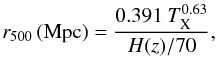 (A.1)where
 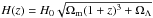 describes the redshift evolution of the Hubble parameter in the assumed cosmological model. Then we use r200 = r500/0.661 corresponding to a Navarro et al. (1997) profile with a halo concentration parameter c = 5.
For clusters with no TX measurements (XLSSC 007, XLSSC 014, and XLSSC 016), we estimate r200 from the cluster velocity dispersion σv, from Willis et al. (2005), following the formula ![Mathematical equation: \appendix \setcounter{section}{1} \begin{equation} r_{200} \, \mathrm{(Mpc)}= \frac{\sqrt{3} \ \sigma_v\mathrm{[km \,s}^{-1}] }{10 \ H(z)} \times 0.85. \label{eq:r200_sigma} \end{equation}](/articles/aa/full_html/2012/07/aa19091-12/aa19091-12-eq232.png) (A.2)This equation is similar to the classical equation for a spherical collapse model (e.g., Carlberg et al. 1997), but for the multiplicative coefficient 0.85. This coefficient comes from a calibration we perform with a compilation of clusters having TX and σv measurements (see for instance Proctor et al. 2011 for a similar systematic difference). Equation (A.2) ensures that there is no bias between our r200 estimated with TX or σv (see Fig. A.1).
(A.2)This equation is similar to the classical equation for a spherical collapse model (e.g., Carlberg et al. 1997), but for the multiplicative coefficient 0.85. This coefficient comes from a calibration we perform with a compilation of clusters having TX and σv measurements (see for instance Proctor et al. 2011 for a similar systematic difference). Equation (A.2) ensures that there is no bias between our r200 estimated with TX or σv (see Fig. A.1).
 |
Fig. A.1 Comparison of r200 estimated with Eqs. (A.1) and (A.2): the test sample is made of 10 clusters from the XMMLSS survey (Willis et al. 2005; Andreon et al. 2006; Pacaud et al. 2007), 28 clusters from the CAIRNS survey (Rines & Diaferio 2006), and 15 clusters from the CNOC1 (Muzzin et al. 2007) and spans 0.003 < zspec < 0.84, 0.5 < TX(keV) < 10.3 and 232 < σv (km s-1) < 1354. There is no bias between the r200 estimated from TX and from σv. The horizontal (resp. vertical) arrows indicate the r200 estimated from TX (resp. σv) for our cluster sample. |
Appendix B: r-band prior for photometric redshifts
Because Eazy has been developed for high-z studies, the r-band prior does not include magnitudes brighter than 20. In our SDSS sample, we deal with galaxies as bright as r ≃ 12. We built the prior probabilities p(z | m0) for 13.5 < r < 18 as follows. For each interval of 0.5 mag, we retrieved ~ 10 000 spectroscopic galaxies from the SpecPhoto view from the SDSS DR8 database and fitted the redshift distribution with a function ![Mathematical equation: \appendix \setcounter{section}{2} \begin{equation} p(z | m_0) \propto z ^{\gamma} \ \exp{[-(z/z_0)^\gamma]}, \label{eq:r_prior} \end{equation}](/articles/aa/full_html/2012/07/aa19091-12/aa19091-12-eq242.png) (B.1)as in Brammer et al. (2008). At 13.5 < r and 18 < r < 20, we visually extrapolated z0 and γ (cf. Fig. B.1), because either there are not enough galaxies or those present in the SDSS are a biased sample (e.g., LRGs, QSOs, etc.).
(B.1)as in Brammer et al. (2008). At 13.5 < r and 18 < r < 20, we visually extrapolated z0 and γ (cf. Fig. B.1), because either there are not enough galaxies or those present in the SDSS are a biased sample (e.g., LRGs, QSOs, etc.).
All Tables
Systematic offsets mfit − mmeas between measured and best-fit model magnitudes for photometric redshift estimation.
All Figures
|
Fig. 1 TX as a function of redshift for our cluster sample. |
| In the text | |
|
Fig. 2 CFHTLS W1 cluster subsample: spatial location of the 18 clusters of our CFHTLS W1 subsample (red crosses). The magenta dashed lines represents CFHTLS W1 fields. For each cluster, blue circles have radii of 0.5 × , 1 × and 2 × r200. Gray areas represent masked regions for fblue estimation and background estimation, due to image corruption (rectangles) or potential clusters at similar redshifts as those of our cluster subsample for each field (disks and sectors). |
| In the text | |
|
Fig. 3 SDSS cluster subsample: spatial location of the seven clusters of our SDSS subsample (red crosses). Magenta/red solid lines represent our SDSS field used for background estimation for each cluster (see Sect. 3.2). For each cluster, blue circles have radii of 0.5 × , 1 × and 2 × r200. Gray areas represent masked regions for fblue estimation and background estimation, due to large-scale structures or potential clusters at similar redshifts as those of our cluster subsample for each field. |
| In the text | |
|
Fig. 4 Illustration of the selection criterion applied in Eqs. (1) and (2) with zcl = 0.61: we display p(z) for three galaxies. For each galaxy, we report above the value for I1 (resp. I2), the integral in Eq. (1) (resp. Eq. (2)), and whether the galaxy is selected or not. Vertical green solid and dashed lines represent zcl and zcl ± 0.05 × (1 + zcl), respectively. |
| In the text | |
|
Fig. 5 Cumulative p(z) function for all objects in background area for four clusters, before (black curves) and after (magenta curves) applying the selection described by Eqs. (1) and (2). Vertical green solid and dashed lines represent zcl and zcl ± 0.05 × (1 + zcl), respectively. |
| In the text | |
|
Fig. 6 (u − r)-like rest-frame probed color: for each cluster of our sample, we plot the rest-frame probed color as a function of the redshift. The shaded areas indicate the wavelength intervals where the filter response convolved with a typical elliptical galaxy spectrum is above half of its maximum value. The vertical bars represent the same for the redshifts of our clusters and the corresponding chosen filters. |
| In the text | |
|
Fig. 7 Dependence of fblue on the rest-frame probed color. Top: like Fig. 6, but for B − V rest-frame color. Bottom: we compare the estimated fblue when using the rest-frame B − V and u − r colors for 84 estimated values (10 clusters for which are available independent filter pairs probing the rest-frame B − V and u − r colors, 1 to 4 mass bins, 3 radial bins). We stress that some individual estimates of fblue have large error bars (see Fig. 10): the 68% shortest intervals for fblue(B − V) and fblue(u − r) all intersect. |
| In the text | |
|
Fig. 8 Illustration of a mass bin definition (zobs = 0.49, 10.73 ≤ log (M/M⊙) < 11.13): thick magenta solid lines represent the loci of constant mass M used in this study (the mass evolved to z = 0), thick blue dashed lines the loci of constant mass Mzobs in stars at zobs, and gray shaded areas represent the difference between those two definitions. The horizontal dotted line represents the threshold used to define blue/red galaxies. |
| In the text | |
|
Fig. 9 Model rest-frame u − r color evolution for different exponentially declining τ-SFHs (CB07 models, solar metallicity and zform = 5). According to our definition a galaxy is classified as red (resp. blue) if it is redder (resp. bluer) than a model with τ = 3.7 Gyr. The vertical arrows indicate the redshifts of our cluster sample. |
| In the text | |
|
Fig. 10 fblue for individual clusters as a function of cluster-centric distance (r/r200) for different bins of redshift (increasing rightward) and galaxy mass (increasing downward). The computed value of fblue already takes into account the mean aging of stars with increasing redshift by defining the color compared to an exponentially declining SFH model with τ = 3.7 Gyr. Error bars represent the shortest interval including 68% of the possible posterior values for fblue, and are plotted as a dashed line when this interval is larger than 0.66, indicating that fblue is not constrained at all. Radial cluster-centric bins are indicated by gray filled triangles on the x-axis and horizontal gray dashed lines indicate the minimum and maximum allowed values for fblue. |
| In the text | |
|
Fig. 11 fblue for stacked clusters as a function of cluster-centric distance (r/r200) for different bins of redshift (increasing rightward) and galaxy mass (increasing downward). The computed value of fblue already takes into account the mean aging of stars with increasing redshift by defining the color compared to an exponentially declining SFH model with τ = 3.7 Gyr. Error bars represent the shortest interval including 68% of the possible posterior values for fblue. Radial cluster-centric bins are indicated by gray filled triangles on the x-axis and horizontal gray dashed lines indicate the minimum and maximum allowed values for fblue. Yellow shaded areas with a solid blue line represent the posterior mean and 68% confidence interval of the modeling of Eq. (3), fitting the 225 individual fblue measurements. Yellow slanting hatched areas with a dashed blue line represent the prediction/extrapolation of this model for bins where we do not have data. Cyan vertically hatched areas with solid magenta line (in two panels only) illustrate how the model fit fails if the ζ term in Eq. (3) is not included. |
| In the text | |
|
Fig. 12 For each parameter fitted with the model of Eq. (3), we plot as a black lines the posterior probability function and as yellow shaded area the shortest interval including 68% of the possible posterior values. We report the point estimate and the 68% confidence interval on each panel, and overplot as a thick red line the corresponding Gaussian curve. The blue lines represent the uniform prior used for the fit. |
| In the text | |
|
Fig. 13 Dependence of fblue on M and z at fixed r/r200 (panels a and b), on z and r/r200 at fixed M (panel c), and on M and r/r200 at fixed z (panel d). Data points with error bars are the same as in Fig. 11. Shaded areas represent the posterior mean and 68% confidence interval of the modeling of Eq. (3), fitting the 225 individual fblue measurements. Prediction/extrapolation of this model for bins where we do not have data are plotted as hatched areas and dashed lines. X-axis bins are indicated by gray filled triangles on the x-axis and horizontal gray dashed lines indicate the minimum and maximum allowed values for fblue. |
| In the text | |
|
Fig. 14 Evolution of fblue for individual (top panels) and stacked (bottom panels) clusters as a function of cluster-centric distance (r/r200) for different bins of redshift (increasing rightward) for a mass-selected sample with a mass corresponding to the original MV in Butcher & Oemler (1984). Symbols are as in Figs. 10 and 11. We add a new panel at z = 1.05 for model prediction, where we overplot the measured values of fblue for the RzCS 052 cluster in Andreon et al. (2008). |
| In the text | |
|
Fig. A.1 Comparison of r200 estimated with Eqs. (A.1) and (A.2): the test sample is made of 10 clusters from the XMMLSS survey (Willis et al. 2005; Andreon et al. 2006; Pacaud et al. 2007), 28 clusters from the CAIRNS survey (Rines & Diaferio 2006), and 15 clusters from the CNOC1 (Muzzin et al. 2007) and spans 0.003 < zspec < 0.84, 0.5 < TX(keV) < 10.3 and 232 < σv (km s-1) < 1354. There is no bias between the r200 estimated from TX and from σv. The horizontal (resp. vertical) arrows indicate the r200 estimated from TX (resp. σv) for our cluster sample. |
| In the text | |
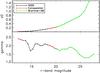 |
Fig. B.1 z0 and γ parameters used for building r-band prior with Eq. (B.1). |
| In the text | |
Current usage metrics show cumulative count of Article Views (full-text article views including HTML views, PDF and ePub downloads, according to the available data) and Abstracts Views on Vision4Press platform.
Data correspond to usage on the plateform after 2015. The current usage metrics is available 48-96 hours after online publication and is updated daily on week days.
Initial download of the metrics may take a while.