| Issue |
A&A
Volume 542, June 2012
|
|
|---|---|---|
| Article Number | A106 | |
| Number of page(s) | 15 | |
| Section | Cosmology (including clusters of galaxies) | |
| DOI | https://doi.org/10.1051/0004-6361/201218979 | |
| Published online | 14 June 2012 | |
Probing cluster dynamics in RXC J1504.1-0248 via radial and two-dimensional gas and galaxy properties
1
Argelander-Institut für Astronomie, Universität Bonn,
Auf dem Hügel 71,
53121
Bonn,
Germany
e-mail: This email address is being protected from spambots. You need JavaScript enabled to view it.
2
Max-Planck-Institut für extraterrestrische Physik,
Giessenbachstraße,
85748
Garching,
Germany
3
University of Vienna, Department of Astronomy,
Türkenschanzstraße 17,
1180
Vienna,
Austria
Received:
7
February
2012
Accepted:
12
April
2012
Abstract
We study one of the most X-ray luminous cluster of galaxies in the REFLEX survey, RXC J1504.1-0248 (hereafter R1504; zcl = 0.2153), using XMM-Newton X-ray imaging spectroscopy, VLT/VIMOS optical spectroscopy, and WFI optical imaging. The mass distributions were determined using both the so-called hydrostatic method with X-ray imaging spectroscopy and the dynamical method with optical spectroscopy, respectively, which yield M500H.E. = (5.81±0.49)×1014 M⊙ and M500caustic = (4.17±0.42)×1014 M⊙. According to recent calibrations, the richness-derived mass estimates closely agree with the hydrostatic and dynamical mass estimates. The line-of-sight velocities of spectroscopic members reveal a group of galaxies with high velocities (>1000 km s-1) at a projected distance of about r500H.E. = (1.18±0.03) Mpc south-east of the cluster centroid, which is also indicated in the X-ray two-dimensional (2D) temperature, density, entropy, and pressure maps. The dynamical mass estimate is 80% of the hydrostatic mass estimate at r500H.E.. It can be partially explained by the ~20% scatter in the 2D pressure map that can be propagated into the hydrostatic mass estimate. The uncertainty in the dynamical mass estimate caused by the substructure of the high velocity group is ~14%. The dynamical mass estimate using blue members is 1.23 times that obtained using red members. The global properties of R1504 obey the observed scaling relations of nearby clusters, although its stellar-mass fraction is rather low.
Key words: cosmology: observations / galaxies: clusters: individual: RXC J1504.1-0248 / galaxies: clusters: intracluster medium / methods: data analysis / X-rays: galaxies: clusters / galaxies: kinematics and dynamics
© ESO, 2012
1. Introduction
Simulations show that the formation of galaxy clusters is not a purely gravitational process. For instance, the galaxy velocity dispersion in clusters provides evidence of heating when compared to the cold dark matter velocity dispersion normalized to the WMAP result and large-scale structure distributions (e.g. Evrard et al. 2008). Cluster mergers do not only disturb the X-ray appearance of the hot intracluster medium (ICM; e.g. Ricker & Sarazin 2001; Poole et al. 2006; Zhang et al. 2009; Böhringer et al. 2010), but also affect the properties of the cluster galaxies (e.g. Sun et al. 2007). The ICM and galaxies react on different timescales during merging (e.g. Roettiger et al. 1999). Clusters with similar X-ray global properties can contain rather different galaxy populations (e.g. Popesso et al. 2007). There is a higher fraction of blue galaxies in rich galaxy clusters at z ≳ 0.2 than in local clusters (Butcher & Oemler 1978, the so-called Butcher-Oemler effect). This effect may be due to episodes of star formation in a subset of cluster members driven by merging (e.g. Saintonge et al. 2008). The kinematic analysis thus complements the X-ray analysis in probing the dynamical structure of a cluster and the consequences of this for the mass measurement.
Comparisons between X-ray and weak-lensing mass estimates suggest that there is a 10–20% deviations from hydrostatic equilibrium at r500 for relaxed clusters of galaxies, and yield controversial findings for disturbed clusters based on different observations (e.g. Zhang et al. 2008, 2010; Mahdavi et al. 2008). The comparison between the X-ray hydrostatic and optical dynamical mass measurements complements the X-ray versus weak-lensing mass comparison, and can thus cross check deviations from hydrostatic equilibrium. Lensing is strongly affected by projection effects because it is sensitive to all mass along the line-of-sight. Line-of-sight velocities of cluster galaxies via the redshifts of cluster galaxies can probe substructures along the line-of-sight. Even for undisturbed clusters, the dynamically relaxed central regions are surrounded by infalling regions in which galaxies are bound to the clusters but not in equilibrium (e.g. Biviano et al. 2006; Rines & Diaferio 2006). Optical spectroscopy can constrain the dynamical properties out to large radii (e.g. Braglia et al. 2007; Ziparo et al. 2012), where it is difficult to probe with current X-ray satellites. On the other hand, X-ray data can be used to derive two-dimensional (2D) cluster morphology projected on the sky. We use these two tools together with the optical colour information to constrain substructures, and model causes of deviations from hydrostatic equilibrium.
RXC J1504.1-0248 (hereafter R1504; zcl = 0.2153), a prominent cool-core cluster, is one of the most relaxed clusters in the REFLEX galaxy cluster survey (Böhringer et al. 2001). Böhringer et al. (2005) investigated the central region of R1504 with Chandra, and found that the core region of R1504 appears to be quite relaxed. Using optical data obtained from integral field spectroscopy and X-ray data from XMM-Newton, Ogrean et al. (2010) found that feedback from active galactic nuclei (AGN) can slow down the cooling flow to the observed mass deposition rate in R1504, if the black-hole accretion rate is of the order of 0.5 M⊙ yr-1 with 10% energy output efficiency. The XMM-Newton data in the R1504 field cover about a two times larger radial range than the Chandra data, and the large effective area of XMM-Newton ensures high quality photon statistics for a 2D spectral analysis. Follow-up observations of R1504 were also performed by the ESO Visible Multi-Object Spectrograph at the 8.2 m UT3 of the Very Large Telescope (VLT/VIMOS) out to about 3r500. In addition, we have at our disposal optical imaging data from the ESO Wide-Field Imager (WFI) in three bands and Subaru in two bands.
We present our analysis of both the radial and 2D gas and galaxy properties of R1504 based on XMM-Newton, VLT/VIMOS, and WFI data as follows. We describe the X-ray analysis and results in Sect. 2, and optical spectroscopic and imaging analyses and results in Sects. 3 and 4. We discuss the systematic uncertainties in and interpretations of the results in Sect. 5. In Sect. 6, we summarize our conclusions. Throughout the paper, we assume that Ωm = 0.3, ΩΛ = 0.7, and H0 = 70 km s-1 Mpc-1. Thus, an extent of 1′ at the distance of R1504 corresponds to 209.8 kpc. Confidence intervals correspond to the 68% confidence level.
2. X-ray data analysis and results
2.1. XMM-Newton observations and data preparation
The XMM-Newton observations (ID: 0401040101) were taken in 2007 with a thin filter in full frame (FF) mode for MOS and extended full frame (EFF) mode for pn. The fraction of out-of-time (OOT) effects amounts to 2.32%, which we used to normalize the pn OOT product before subtracting it from the pn normal product.
We applied an iterative 2σ clipping procedure (e.g. Sect. 2.1 of Zhang et al. 2006) to filter flares using the light curves in both the soft band (0.3–10 keV) binned in 10 s intervals and the hard band (10–12 keV for MOS and 12–14 keV for pn) binned in 100 s intervals. There are 34.9 ks clean data for MOS1, 34.5 ks for MOS2, and 31.6 ks for pn left. We generated a list of bright point sources detected with the XMMSAS task edetect_chain applied to five energy bands: 0.3–0.5 keV, 0.5–2 keV, 2–4.5 keV, 4.5–7.5 keV, and 7.5–12 keV. All confirmed sources were subtracted from the event lists using a radius of 25′′, which encloses ~80% of the flux of the point sources according to the XMM-Newton point spread function (PSF). A weight column was created with the XMMSAS evigweight command, which accounts for the vignetting correction for off-axis observations.
2.2. Temperature and surface brightness distributions
Following Sect. 2.3 of Zhang et al. (2010), we
measured the X-ray flux-weighted centroid to be
RA = 15h04m07 801,
δ = −02°48′10
801,
δ = −02°48′10 29 (J2000). We
applied the double-background subtraction method developed for clusters at similar
redshifts by Zhang et al. (2006, the so-called DBS
II method therein). We chose the XMM-Newton blank sky accumulations in
the Chandra Deep Field South (CDFS), which used the medium filter and
were also acquired in FF/EFF mode for MOS/pn as R1504, as background observations. The
count rate in the hard band was used to normalize the CDFS observations before subtracting
them from the target observations. The cluster X-ray emission was confined to be within
R < 6′, so that we use the annulus region
outside R = 8′ to probe the residual background and subtract it, taking
into account the area correction for gaps and point sources. We chose the bin size of each
annulus for the spectral extraction to be ≥ 0
29 (J2000). We
applied the double-background subtraction method developed for clusters at similar
redshifts by Zhang et al. (2006, the so-called DBS
II method therein). We chose the XMM-Newton blank sky accumulations in
the Chandra Deep Field South (CDFS), which used the medium filter and
were also acquired in FF/EFF mode for MOS/pn as R1504, as background observations. The
count rate in the hard band was used to normalize the CDFS observations before subtracting
them from the target observations. The cluster X-ray emission was confined to be within
R < 6′, so that we use the annulus region
outside R = 8′ to probe the residual background and subtract it, taking
into account the area correction for gaps and point sources. We chose the bin size of each
annulus for the spectral extraction to be ≥ 0 5 and to have
about 4000 net counts in the 2–7 keV band. The former ensures a redistribution fraction of
less than 20% of the flux obtained within each annulus, and the latter ensures no more
than 20% errors in the temperature measurements. Figure 1 shows the X-ray spectra extracted from the central
≤ 05 circle. The
spectra were fitted with the XSPEC software using the combined mekal ∗ wabs model, in
which the former describes the ICM emission, and the latter describes the Galactic
absorption with a Galactic hydrogen column density of nH. We
freeze the cluster redshift to 0.2153 and nH to the value of
6.08 × 1020 cm-2 given by the LAB survey (Hartmann &
Burton 1997; Arnal et al. 2000; Bajaja et al. 2005; Kalberla
et al. 2005) at the X-ray flux-weighted centroid.
5 and to have
about 4000 net counts in the 2–7 keV band. The former ensures a redistribution fraction of
less than 20% of the flux obtained within each annulus, and the latter ensures no more
than 20% errors in the temperature measurements. Figure 1 shows the X-ray spectra extracted from the central
≤ 05 circle. The
spectra were fitted with the XSPEC software using the combined mekal ∗ wabs model, in
which the former describes the ICM emission, and the latter describes the Galactic
absorption with a Galactic hydrogen column density of nH. We
freeze the cluster redshift to 0.2153 and nH to the value of
6.08 × 1020 cm-2 given by the LAB survey (Hartmann &
Burton 1997; Arnal et al. 2000; Bajaja et al. 2005; Kalberla
et al. 2005) at the X-ray flux-weighted centroid.
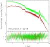 |
Fig. 1 MOS1 (black), MOS2 (red), and pn (green) spectra extracted from the central
≤ 0 |
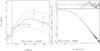 |
Fig. 2 Left: deprojected temperature measurement versus radius with the
parametrized temperature distribution indicated by the solid curve and the
1σ interval by the dashed curves. The vertical line denotes
|

The left panel of Fig. 2 shows that the radial temperature distribution follows the universal profile of relaxed clusters (e.g. Markevitch et al. 1998; Vikhlinin et al. 2006; Zhang et al. 2006; Pratt et al. 2007). The observed strong cool core is also shown in Chandra data by Böhringer et al. (2005). The amplitude of the temperature distribution is, however, 20% lower than that of the Chandra measurements. Snowden et al. (2008) found that temperature measurements with Chandra are overestimated for those that are hotter than 5 keV owning to a calibration problem, which was corrected only recently with Chandra CALDB v3.5.2. The temperature overestimation made by analyses of previous Chandra CALDB thus accounts for the amplitude difference between the temperature distributions measured with Chandra by Böhringer et al. (2005) and with XMM-Newton in this work. The right panel of Fig. 2 shows the surface brightness distribution. We carried out the PSF deconvolution and deprojection as detailed in Sect. 2.3 of Zhang et al. (2007), in which the XMM-Newton PSF matrices were created according to Ghizzardi (2001).
2.3. Mass distribution using the hydrostatic method
We assumed that the ICM is in hydrostatic equilibrium within the gravitational potential
dominated by dark matter, and that the matter distribution is spherically symmetric. The
mass could thus be calculated from the X-ray measured radial density and temperature
distributions of the ICM by ![Mathematical equation: \begin{equation} \frac{1}{\mu m_{\rm p} n_{\rm e}(r)}\frac{{\rm d}[n_{\rm e}(r) k T(r)]}{{\rm d}r}= -\frac{GM(\le r)}{r^2}\,, \end{equation}](/articles/aa/full_html/2012/06/aa18979-12/aa18979-12-eq37.png) (1)in which
μ = 0.62 is the mean molecular weight per hydrogen atom, and
k is the Boltzmann constant. The mass estimate was computed from a set
of input parameters β, ne0i,
and rci (i = 1,2)
representing the double-β electron number-density profile
(1)in which
μ = 0.62 is the mean molecular weight per hydrogen atom, and
k is the Boltzmann constant. The mass estimate was computed from a set
of input parameters β, ne0i,
and rci (i = 1,2)
representing the double-β electron number-density profile
 , and
Pi (i = 1,...,7)
representing the deprojected temperature profile,
, and
Pi (i = 1,...,7)
representing the deprojected temperature profile, ![Mathematical equation: \hbox{$T(r)=P_3\exp[-(r-P_1)^2 P_2^{-1}]+P_6(1+r^2 P_4^{-2})^{-P_5}+P_7$}](/articles/aa/full_html/2012/06/aa18979-12/aa18979-12-eq47.png) . We propagated the
uncertainties in the electron number-density and temperature measurements using Monte
Carlo simulations to compute the mass uncertainty. The cluster radius
rΔ (e.g. r500) was defined as
the radius within which the mass density is Δ (e.g. 500) times of the critical density at
the cluster redshift,
. We propagated the
uncertainties in the electron number-density and temperature measurements using Monte
Carlo simulations to compute the mass uncertainty. The cluster radius
rΔ (e.g. r500) was defined as
the radius within which the mass density is Δ (e.g. 500) times of the critical density at
the cluster redshift, 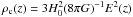 , in
which
E2(z) = Ωm(1 + z)3 + ΩΛ + (1 − Ωm − ΩΛ)(1 + z)2.
, in
which
E2(z) = Ωm(1 + z)3 + ΩΛ + (1 − Ωm − ΩΛ)(1 + z)2.
Basic properties of R1504.
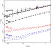 |
Fig. 3 Cumulative mass distributions (1) using the X-ray hydrostatic method (filled
squares), (2) using the caustic method (black solid curve), (3) of the gas mass
estimate (black dotted curve), (4) of the stellar mass estimate of the red galaxies
(red dash-dotted curve), and (5) of the stellar mass estimate of the blue galaxies
(blue dash-dotted-dotted-dotted curve). The dashed curves and error bars denote
1σ intervals. The open star, triangle, diamond, and circle
indicate the dynamical mass estimates ( |


The cumulative mass distribution using the hydrostatic method is shown in Fig. 3 as filled squares. The cluster radius is
 Mpc,
and the total mass estimate is
Mpc,
and the total mass estimate is  as listed in
Table 1. The mass profile can be well-fitted by
an NFW model (Navarro et al. 1997) with a
concentration parameter of c500 = 2.93 ± 0.14.
as listed in
Table 1. The mass profile can be well-fitted by
an NFW model (Navarro et al. 1997) with a
concentration parameter of c500 = 2.93 ± 0.14.
2.4. Two-dimensional spectrally measured maps
We adopted the adaptive-binning methods developed by Sanders (2006) and Cappellari & Copin (2003; see also Diehl & Statler 2006), respectively, to define the masks for the 2D analysis. We followed the steps in Sect. 5 of Zhang et al. (2009), except for two changes: (i) we adopted a threshold of signal-to-noise ratio (S/N) of 30 instead of 45 to ensure an adequate number of bins in the mask. (ii) We used the double-background subtraction strategy (i.e. DBS II) since there is a sufficient outer area within the XMM-Newton field of view (FoV) to model the residual background.
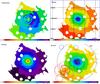 |
Fig. 4 Two-dimensional X-ray spectrally measured temperature (upper
left), electron number-density (upper right), entropy
(lower left), and pressure (lower right) maps
using the Sanders (2006) binning scheme.
Overlaid circles in blue, red, and green denote cluster galaxies that have
spectroscopic follow-up data with their clustercentric velocities toward the
observer greater than 1000 km s-1, away from the observer greater than
1000 km s-1, and smaller than 1000 km s-1, respectively. The
radii of these circles are proportional to |
The X-ray spectrally measured 2D maps using the Sanders (2006) mask are shown in Fig. 4. Those using
the Cappellari & Copin (2003) mask appear
in Fig. A.1. At a projected distance of
~ south-east of the centroid, the surface brightness shows a clump with its value 2.25 times
the azimuthal average of
(2.4 ± 0.4) × 10-3 counts s-1 arcmin-2, at the same
projected distance. This enables us to carry out the 2D spectral analysis toward larger
radii in the south-east direction than the other directions. In the temperature map, we
also observe a hot stripe at ~
south-east of the centroid, the surface brightness shows a clump with its value 2.25 times
the azimuthal average of
(2.4 ± 0.4) × 10-3 counts s-1 arcmin-2, at the same
projected distance. This enables us to carry out the 2D spectral analysis toward larger
radii in the south-east direction than the other directions. In the temperature map, we
also observe a hot stripe at ~ west
of the centroid.
west
of the centroid.
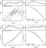 |
Fig. 5 Temperature (upper left), electron number-density (upper right), entropy (lower left), and pressure (lower right) distributions of the spectrally measured 2D maps using the Sanders (2006) binning scheme are shown as crosses with their local regression fits in black curves. The solid and dashed grey curves in the upper left plot show the parametrization of the deprojected temperature profile and its 1-σ interval derived in Sect. 2.3. Differential scatter and its 1-σ intervals of the temperature, electron number-density, entropy, and pressure fluctuations in the 2D maps are shown in solid and dashed black curves in their upper panels. |
We followed Zhang et al. (2009) to calculate the
scatter in the fluctuations in the 2D maps and analyse the ICM substructure. In Fig. 5, the temperature, electron number-density, entropy, and
pressure distributions in the 2D maps are shown as a function of projected distance from
the X-ray flux-weighted centroid. Their non-parametric locally weighted regression (e.g.
Becker et al. 1988) was used as the mean profile.
The differential scatter and error were calculated from the area-weighted absolute
fluctuations with all bins at that projected distance. The temperature, electron
number-density, entropy and pressure maps have scatters of smaller than ~15%, 30%, 20%,
and 25%, respectively. The scatter in the temperature measurements increases with radius,
and is ~12% at the radii beyond . In
contrast, the electron number-density measurements appear to have a smaller scatter at
large radii, which may reflect the different relaxation timescales of the ICM temperature
and electron number density.
The 2D maps using the Cappellari & Copin (2003) mask demonstrate a mild elongation along the east-west major axis on the
scale of ~.
3. Optical spectroscopic data analysis and results
3.1. VLT/VIMOS observations and data preparation
Multi-object spectroscopy in the R1504 field was performed with the VLT/VIMOS spectrograph using the low-resolution blue grism (LR-blue) with the OS-blue filter, which samples the [3700–6700] Å wavelength range with λ/Δλ = 180 (PID: 077.A-0058). The observations were carried out in service mode, which include a bias, dark, and flat calibration sequence with the last of these using the same set-up as the observations.
The cluster R1504 was observed with air masses of between 1.124 and 1.172. The seeing was
less than 15 for two
pointed observations and >2′′ for one pointed
observation. Individual targets for the spectroscopic follow-up were selected based on
their I-band magnitudes in the pre-imaging data. In total, 784 slits were
placed in the 12 masks spread over three pointed observations.
Data were reduced with the VIPGI pipeline (Scodeggio et al. 2005). Redshifts were computed by comparing the observed spectra to galaxy and stellar templates with the EZ software (Garilli et al. 2010) and improved with customized tools from Verdugo et al. (2008) by fitting a Gaussian profile to each of the observed strong spectral features. Not all lines, namely [O ii] λλ3726, 3729 ÅÅ, [Ca ii K] λ3934 Å, [Ca ii H] λ3968 Å, Hδ λ4102 Å, Hβ λ4861 Å, G-band (~λ4304 Å), [O iii] λλ4959, 5007 ÅÅ, Mg 1b (~5050–5430 Å), and [Fe vi] λ5335 Å, are present in each spectrum. The redshift determined from each spectrum is the mean of the individual shifts for all visible line features. The error is the standard deviation in these shifts, which takes into account systematic errors in the wavelength calibration and differences in the S/N. The average error in the individual redshift estimates is Δz = 0.00076.
The R1504 field overlaps with the stellar stream of the globular cluster Palomar-5 (e.g. Odenkirchen et al. 2001). There are thus a large number of white- and red-dwarf stars contaminating the spectroscopic sample. Interlopers were removed by applying the member selection procedure in Sect. 3.2.
3.2. Spectroscopic member selection
In hierarchical structure-formation scenarios, the spherical infalling model predicts a trumpet-shaped region in the diagram of line-of-sight velocity versus projected distance, the so-called caustic (e.g. Kaiser 1987). The boundary defines galaxies inside the caustic as cluster members and those outside the caustic as fore- and background galaxies.
Several methods can select cluster members according to their line-of-sight velocities. A constant gap or gaps weighted by projected distances can separate member galaxies from fore- and background galaxies (e.g. Beers et al. 1990; Girardi et al. 1993; den Hartog & Katgert 1996; Katgert et al. 1996, 2004; Popesso et al. 2005a; Biviano et al. 2006). Alternatively, an adaptive kernel method, sensitive to the presence of peaks, has been widely used to select members (e.g. Pisani 1993, 1996; Fadda et al. 1996; Diaferio & Geller 1997; Diaferio 1999; Geller et al. 1999; Rines & Diaferio 2006).
We modified the adaptive kernel method of Diaferio (1999) for medium-distance clusters (e.g. Harrison & Noonan 1979; Danese et al. 1980), and used it to identify the interlopers as follows. Galaxies with
redshifts
|cz − czcl| ≤ 4000 km s-1
were preliminarily selected and located in the (r,v) diagram, where
r is the galaxy transverse separation from the cluster centroid, and
v is the line-of-sight velocity of the galaxy relative to the cluster.
At the redshift of R1504, we modified the calculation of (r,v) to
r = Dasinθ and
v = (cz − czclcosθ)/(1 + zcl),
where Da, θ, z,
and zcl are the angular diameter distance of the cluster,
angular separation of the galaxy from the cluster centroid, galaxy redshift, and cluster
redshift. The angular diameter distance is defined as
 . We
scaled r and v to ensure approximately equal weights in
r and v, and computed the 2D adaptive density
distribution f(r,v). The boundary of the caustic is
defined by f(r,v) = κ, in which
κ is determined by minimizing
. We
scaled r and v to ensure approximately equal weights in
r and v, and computed the 2D adaptive density
distribution f(r,v). The boundary of the caustic is
defined by f(r,v) = κ, in which
κ is determined by minimizing  . Here
 is the escape velocity,
R and ⟨ v2 ⟩ R
are the mean projected distance and velocity dispersion of the members, and
ϕ(r) = ∫f(r,v)dv.
In addition,
is the escape velocity,
R and ⟨ v2 ⟩ R
are the mean projected distance and velocity dispersion of the members, and
ϕ(r) = ∫f(r,v)dv.
In addition,  ,
which represents the minimum of the upper and lower solutions of
f(r,v) = κ.
,
which represents the minimum of the upper and lower solutions of
f(r,v) = κ.
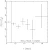 |
Fig. 6 Radial distribution of the iron abundance. The vertical line
denotes |
Figure 7 shows the histogram of the line-of-sight velocity and the diagram of line-of-sight velocity versus projected distance of galaxies. The 53 galaxies inside the caustic boundary are considered as members. Our further dynamical analysis is based on these 53 spectroscopic member galaxies.
3.3. Mass distribution using the caustic method
We applied the biweight estimator developed by Beers et al. (1990) to measure the redshift and velocity dispersion, in which the errors are estimated by means of 1000 bootstrap simulations. The cluster redshift was assumed to be the biweight estimator of location of the recessional velocities, czi. The velocities in the cluster reference frame vrest,i were derived from the recessional velocities czi using the formula vrest,i = (czi − czcl)(1 + zcl)-1. The velocity dispersion was given by the biweight estimator of scale of these vrest,i values. With all 53 spectroscopic members, the measured redshift is (0.2165 ± 0.0005), and the velocity dispersion is (1132 ± 94) km s-1.
The escape velocities of galaxies extracted from the amplitude of the caustic scale with
the gravitational potential of the dark matter halo (e.g. Diaferio & Geller 1997; Diaferio 1999; Rines & Diaferio 2006)
 (2)The error in the
cumulative mass estimate within ri is defined
as
(2)The error in the
cumulative mass estimate within ri is defined
as  , in
which mj is the mass estimate in the
jth shell,
, in
which mj is the mass estimate in the
jth shell,  ,
and max { f(r,v) } is the maximum value of
f(r,v) at fixed r. Since the caustic
of a spherical system is symmetric, the minimum of the upper and lower caustics is taken
as the caustic amplitude at each radius, which excludes interlopers more effectively than
taking the average of the upper and lower caustics as the caustic amplitude. The caustic
method does not assume dynamical equilibrium, and is thus able to measure cluster masses
out to large radii. The mass distribution using the caustic method is shown in Fig. 3, and implies that
,
and max { f(r,v) } is the maximum value of
f(r,v) at fixed r. Since the caustic
of a spherical system is symmetric, the minimum of the upper and lower caustics is taken
as the caustic amplitude at each radius, which excludes interlopers more effectively than
taking the average of the upper and lower caustics as the caustic amplitude. The caustic
method does not assume dynamical equilibrium, and is thus able to measure cluster masses
out to large radii. The mass distribution using the caustic method is shown in Fig. 3, and implies that
 Mpc
(Table 1).
Mpc
(Table 1).
3.4. Two-dimensional kinematic structure
As clusters of galaxies formed at moderate look-back times, they often contain
substructures caused by the accretion of and merging with smaller systems. The
quantification of substructures is thus important to assess the reliability of different
mass measurements and infer the dynamical history of the cluster. It is, however,
difficult to quantify substructures at large radii with XMM-Newton data
because of the high background level relative to the faint X-ray emission near
.
Optical spectroscopic data provide a promising alternative means of quantifying
substructures at all radii.
Dressler & Shectman (1988, DS hereafter)
developed a statistical method for detecting substructures in galaxy clusters related to
systematic deviations from the average spatial and/or velocity structure, which we
summarize as follows. The deviation in the local velocity mean and dispersion from the
global mean and dispersion of the cluster is defined as
![Mathematical equation: \begin{equation} \rho_{\rm DS}=\sqrt{\frac{N_{\rm local}+1}{ \sigma^{2}} \bigg[(\bar{v}_{\rm local}-\bar{v})^2+(\sigma_{\rm local}-\sigma)^2\bigg]}\,. \end{equation}](/articles/aa/full_html/2012/06/aa18979-12/aa18979-12-eq203.png) (3)The local line-of-sight
velocity and dispersion,
(3)The local line-of-sight
velocity and dispersion,  and σlocal, are measured with its
Nlocal = 10 nearest neighbours in projection. The global
line-of-sight velocity and dispersion,
and σlocal, are measured with its
Nlocal = 10 nearest neighbours in projection. The global
line-of-sight velocity and dispersion,  km s-1
and σ = 1132 km s-1, are given in Sect. 3.3 as measured for all (i.e. Nall = 53 for
R1504) spectroscopic cluster members. A cumulative deviation
km s-1
and σ = 1132 km s-1, are given in Sect. 3.3 as measured for all (i.e. Nall = 53 for
R1504) spectroscopic cluster members. A cumulative deviation
 is of
the order of Nall when the line-of-sight velocity obeys a
Gaussian distribution and local variations are only random fluctuations, but differs from
Nall when the line-of-sight velocity distribution deviates
from a Gaussian. Therefore, the ΔDS statistic is sensitive to the presence of
substructures. A higher ΔDS value indicates a higher possibility of containing
substructures.
is of
the order of Nall when the line-of-sight velocity obeys a
Gaussian distribution and local variations are only random fluctuations, but differs from
Nall when the line-of-sight velocity distribution deviates
from a Gaussian. Therefore, the ΔDS statistic is sensitive to the presence of
substructures. A higher ΔDS value indicates a higher possibility of containing
substructures.
In Fig. 4, we display the 53 spectroscopic galaxies
by circles with their radii proportional to ![Mathematical equation: \hbox{$\exp [\rho_{\rm DS}^2]$}](/articles/aa/full_html/2012/06/aa18979-12/aa18979-12-eq157.png) . The blue, red, and green
colours denote cluster galaxies that have spectroscopic follow-up data with their
clustercentric velocities toward the observer greater than 1000 km s-1, away
from the observer greater than 1000 km s-1, and smaller than
1000 km s-1. The DS test yields ΔDS,obs = 86.8,
and reveals a clustering of galaxies with large ρDS values at
a projected distance of ~
south-east of the cluster centroid. This may be indicative of a relatively high-velocity
(>1000 km s-1) group associated with the main
cluster.
. The blue, red, and green
colours denote cluster galaxies that have spectroscopic follow-up data with their
clustercentric velocities toward the observer greater than 1000 km s-1, away
from the observer greater than 1000 km s-1, and smaller than
1000 km s-1. The DS test yields ΔDS,obs = 86.8,
and reveals a clustering of galaxies with large ρDS values at
a projected distance of ~
south-east of the cluster centroid. This may be indicative of a relatively high-velocity
(>1000 km s-1) group associated with the main
cluster.
To estimate the robustness of the ΔDS statistic, we carried out
nMC = 10 000 Monte Carlo simulations by randomly shuffling
the line-of-sight velocities of the member galaxies. This procedure erases any true
correlations between the line-of-sight velocities and positions. The probability of having
substructures can be estimated by  , in which
δj = ΔDS,j when
ΔDS,j > ΔDS,obs
and δj = 0 otherwise (e.g. Hou et al. 2012). Therefore, systems with significant
substructures show low-PDS values. The Monte Carlo realization
of the ΔDS statistic yields PDS = 0.06 for R1504,
which only corresponds to a ~10% false detection according to Hou et al. (2012). This PDS-value thus
represents a non-negligible possibility that the high velocity group exists. The histogram
of the line-of-sight velocities of possible member galaxies of the high velocity group is
shown as (red) dashed lines in the left panel of Fig. 7.
, in which
δj = ΔDS,j when
ΔDS,j > ΔDS,obs
and δj = 0 otherwise (e.g. Hou et al. 2012). Therefore, systems with significant
substructures show low-PDS values. The Monte Carlo realization
of the ΔDS statistic yields PDS = 0.06 for R1504,
which only corresponds to a ~10% false detection according to Hou et al. (2012). This PDS-value thus
represents a non-negligible possibility that the high velocity group exists. The histogram
of the line-of-sight velocities of possible member galaxies of the high velocity group is
shown as (red) dashed lines in the left panel of Fig. 7.
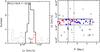 |
Fig. 7 Left: histogram of the line-of-sight velocities. Member galaxies
of the cluster, member galaxies of the high velocity group, and non-member galaxies
are in solid (black), dashed (red), and dash-dotted (grey) lines. The arrow shows
the cluster redshift. Right: line-of-sight velocity versus
projected radius, in which filled blue diamonds and red stars show blue and red
member galaxies in the caustic (black curve), and open squares show fore- and
background galaxies. The grey curve shows the symmetric boundary by choosing the
minimum of the values on both sides of the caustic boundary relative to the cluster
redshift. The cluster radii, |


4. Optical imaging data analysis and results
4.1. WFI observations and data preparation
The cluster R1504 was observed with the ESO/MPG 2.2 m telescope with the WFI (Baade
et al. 1999) in the
B/123-, V/89-,
and Rc/162-bands (hereafter
B-, V-, and R-bands) during three
runs in June 2009, 2010, and 2011 mostly under non-photometric conditions. The WFI has a
4 × 2 mosaic detector of 2k × 4k CCDs, which has a pixel size of
0238 and a FoV of
34′ × 33′. We reduced the data and co-added the single exposures using the THELI
pipeline (Erben et al. 2005). The coadded
B-, V-, and R-band images have total
exposure times of 9238 s, 8317 s, and 11 035 s with
127,
121, and
096 seeing.
Figure 8 shows the WFI B-band
image.
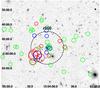 |
Fig. 8 WFI B-band imaging. Overlaid circles in blue, red and green denote
cluster galaxies with spectroscopic follow-up data that have clustercentric
velocities toward the observer greater than 1000 km s-1, away from the
observer greater than 1000 km s-1, and smaller than
1000 km s-1, respectively. The radii of these circles are proportional
to |
Since the observing conditions of the imaging varied slightly, photometric calibration of the WFI R-band data was tied to the shallower SDSS r-band data in the same field. The B- and V-band images were calibrated against the R-band by fitting the observed main sequence of stars with that of a photometrically calibrated field. Cross-checks were applied by comparing predicted with observed colours for galaxies with spectroscopic redshifts using procedures typical of photometric redshift codes. The absolute calibration of the photometric zero point is more accurate than 0.1 mag. The internal colour calibration is more accurate than 0.04 mag.
Photometry was carried out with SExtractor (Bertin & Arnouts 1996) in dual mode with the R-band
image set as the detection frame. Galaxy colours were measured in an aperture of
25 diameter.
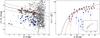 |
Fig. 9 Left: colour–magnitude diagram with the corresponding red sequence
indicated by a solid line and its 3σ = 0.249 magnitude intervals by
dashed lines. The sample is complete down to the curve at ~22 mag, which varies
slightly with the B − R colour. We thus limited
the analysis to the galaxies brighter than R = 22 mag. The dotted
line denotes the colour cut that is 1.5 mag bluer than the red sequence, below which
the objects were considered as foreground contamination. Red stars and blue diamonds
indicate red and blue spectroscopic member galaxies regardless of their
clustercentric distances. The BCG is extremely blue with
B − R = 0.98. Right: cluster
galaxy luminosity functions for red (red stars), blue (blue diamonds), and all
(black circles) members within |
4.2. Photometric member selection
The broad B- and R-bands can probe the spectral range
across the 4000 Å break for galaxy clusters at z ~0.2−0.3, which can
be used to characterize the bulk of stellar populations. Early-type galaxies display red
colours and reside in a narrow band, the so-called red sequence (e.g. Baum 1959), in the colour–magnitude diagram. The
B − R colour versus R-band magnitude
is shown in the left panel of Fig. 9 for all galaxies
within , in
which we highlight the 29 blue and 24 red spectroscopic members regardless of their
clustercentric distances.
We fit the red sequence with a robust biweight linear-fitting algorithm, which is negligibly affected by skewness (e.g. Beers et al. 1990; Gladders et al. 1998). The best-fit relation is B − R = −0.097R + 3.88 with a scatter of σ = 0.083 mag.
We define red members as galaxies within 3σ of the best-fit red sequence. Galaxies that are more than 3σ bluer than the red sequence are considered as blue galaxies, whereas galaxies that are more than 3σ redder than the red sequence are discarded because they are most likely background galaxies. We also discard galaxies bluer by more than 1.5 mag than the red sequence to reduce foreground contamination. These limits are marked in Fig. 9.
The comparison between the galaxy number counts in the R1504 field and the Garching-Bonn Deep Survey (GaBoDS, Erben et al. 2005; Hildebrandt et al. 2006) fields shows that our photometric sample is 100% complete down to R = 22 mag. This limit corresponds to MR ≈ −18 mag for galaxies of different colours at zcl = 0.2153, and is indicated by an oblique curve in Fig. 9. The CLASS_STAR parameter provided by SExtractor is completely reliable down to R = 21.5 mag and 90% reliable down to R = 22 mag. We thus limit the analysis to the galaxies brighter than R = 22 mag. The limiting magnitude is R = 24.44 mag at 5σ, which was calculated in an aperture of 1′′ diameter. The stellar contamination should be quite low in the photometric sample because of the high quality of the WFI imaging.
4.3. Galaxy luminosity function and stellar mass
To determine the photometric properties of the cluster population, we corrected for contamination by both fore- and background galaxies along the line-of-sight by applying a statistical subtraction using a subset (2.25 deg2) of the GaBoDS, whose photometric data are complete in all bands. We applied the same magnitude and colour cuts to the GaBoDS fields as we did to the R1504 field, and constructed the galaxy number counts as a function of magnitude for red and blue galaxies, respectively. The galaxy number counts in the GaBoDS fields were normalized to the R1504 sky area and subtracted from the corresponding galaxy number counts in the R1504 field. The size of the magnitude bin used to construct the galaxy number counts was chosen to be large enough to ensure that there were positive counts in all magnitude bins after subtracting the background. The errors are a combination of the Poisson statistical error and cosmic variance. The latter was measured to be the standard deviation in the galaxy number counts across the GaBoDS fields. The Poisson statistical error dominates the error budget at inner radii because there are relatively fewer objects, whereas cosmic variance dominates at large radii.
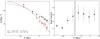 |
Fig. 10 Left: number density profiles with their best-fit NFW models for
red member galaxies (red triangles, solid curve) and all members (black circles,
dashed curve), respectively. We obtained reduced
χ2 = 1.03,2.24 for the red and all
member galaxies, which indicates that the red galaxies follow well the theoretical
profile and the blue galaxies may account for the deviation of the fit for all
member galaxies. The bin size is 300 kpc. Right: ratio of blue to
all member galaxies as a function of projection distance from the X-ray
flux-weighted centroid. The vertical line
remarks |
The right panel of Fig. 9 shows the
R-band galaxy luminosity functions for red (red), blue (blue), and all
(black) members within . We
derived the best-fit Schechter (1976) functions for
red and all members, respectively, with a χ2 minimization
algorithm. The red members show a shallower slope at the faint end than that of all
members. As listed in Table 1, both the
characteristic R-band magnitude, R∗, and
the slope at the faint end, α, agree with that of nearby clusters (e.g.
Christlein & Zabludoff 2003; Popesso et al.
2005b; Durret et al. 2011). No fit was possible for blue galaxies.
The brightest cluster galaxy (BCG) is very blue
(B − R = 0.98) and bright (R = 16 mag).
Since the BCG cannot normally be described by the Schechter function, we explicitly
removed the BCG from the photometric sample in the above calculation of the galaxy
luminosity function. The total R-band luminosity of the cluster was
computed by explicitly adding the BCG luminosity to the integration of the galaxy
luminosity function. We tested how the BCG colour affects the measured optical luminosity
by adding the BCG luminosity to the red and blue populations, respectively. The resulting
uncertainty in the R-band luminosity is smaller than 3%. The measured
R-band optical luminosity within
is
listed in Table 1.
We adopted the stellar mass-to-optical light ratio from Table 7 of Bell et al. (2003),
log (M ∗ /LR) = a + b(B − R),
in which a = −0.523, b = 0.683,
B − R is the rest-frame colour, and a “diet” Salpeter
(1955) stellar initial mass function (Bell
& de Jong 2001) is adopted. We show the
cumulative stellar mass profiles for red and blue galaxies, respectively, in Fig. 3. The stellar mass estimates for blue, red, and all
photometric members within are
given in Table 1. The cluster R1504 has a rather
low stellar-mass fraction among nearby clusters (e.g. Biviano & Salucci 2006), although there is an agreement given the large
scatter for nearby clusters (e.g. Andreon 2010;
Zhang et al. 2011b). The contribution to the total
stellar mass budget associated with intra-cluster light (e.g. Zibetti et al. 2005) could reach 10–20% level at the mass scale of
galaxy groups (e.g. Gonzalez et al. 2007). The difference in the R-band
luminosity caused by adding the BCG luminosity to the blue and red populations,
respectively, is within 3% for R1504. Therefore, both the intra-cluster light and BCG play
non-dominant roles to explain the low stellar-mass fraction.
4.4. Blue-galaxy fraction
Understanding rapid galaxy-morphology transformation is essential to model the mass assembly history of galaxy clusters. Red galaxies with low levels of ongoing star formation are assumed to be the descendants of blue star-forming galaxies that have been accreted from the surrounding filamentary structure and quenched by specific processes operating within the cluster environment (e.g. Braglia et al. 2007; Verdugo et al. 2012). How spirals were transformed into ellipticals remains unclear (e.g. Poggianti & Wu 2000). The efficiency of different transformation processes varies with environment. Ram pressure stripping, for instance, is more effective in the cluster core where there is dense ICM (e.g. Fujita & Nagashima 1999; Quilis et al. 2000). Galaxy-galaxy merging, on the other hand, is more effective in infalling groups at the cluster outskirts (e.g. Kauffmann et al. 1999).
In the left panel of Fig. 10, we present the number
density profiles of the red and all member galaxies, respectively, as a function of
projected distance from the X-ray flux-weighted centroid. Similar to the findings for
other clusters (e.g. Lin et al. 2004), the red
population in R1504 is well-fitted by a projected NFW profile (Navarro et al. 1997; Bartelmann 1996), in which the reduced χ2 is 1.03. The fit of a
projected NFW profile to all members is relatively poor with
χ2 = 2.24. The right panel of Fig. 10 displays the blue-galaxy fraction. Within a projected distance of
700 kpc, where the ICM is dense, the galaxy population is dominated by red galaxies with a
fraction larger than 70%. Beyond 700 kpc, the blue-galaxy fraction first increases
rapidly, reaching 60% at ~, and
then stays almost constant in the outskirts.
The large error bars in the blue-galaxy fraction at large radii take into account the
uncertainty in the background. The colours of the field galaxies have their own variation.
One cannot exclude that the high blue-galaxy fraction is coincidently due to a larger
field-galaxy contamination. A reliable measure of the blue-galaxy fraction free of
background contamination requires extensive spectroscopy. Nevertheless, the high
blue-galaxy fraction beyond may
indicate a critical distance where specific processes in clusters such as starvation (e.g.
Balogh et al. 2000) start to affect the properties
of infalling galaxies. This distance may, however, depend on the environment (e.g.
Urquhart et al. 2010). Urquhart et al. (2010, Fig. 10 therein) pointed out an excess of
extremely blue galaxies in massive groups, in which active starburst galaxies are driven
by galaxy-galaxy interactions in the group environment. The radial blue-galaxy fraction
and presence of the high velocity group in R1504 support this interpretation.
4.5. Richness-derived mass estimates
There are a number of approaches for calculating the cluster total mass based on photometric measurements (e.g. Hansen et al. 2005, 2009; Johnston et al. 2007; Reyes et al. 2008).
We can iteratively estimate the mass from the richness distribution according to existing scaling calibrations between richness and mass estimates at a fixed overdensity. The cluster total mass is measured within the radius where the mass density is 200 times the critical density in Johnston et al. (2007) and Hansen et al. (2009), but 200 times the mean density of the Universe in Hansen et al. (2005) and Reyes et al. (2008). To be consistent with the mass definition, we use the calibrations between richness and weak-lensing mass measurements in Johnston et al. (2007), Eq. (26), and Hansen et al. (2009), Eq. (10), respectively, to calculate the richness-derived mass estimates. In these calibrations, the richness was measured down to 0.4 L∗ in the SDSS i-band, which is equivalent to (i∗ + 1) magnitude. Since there were no i-band data for R1504, we used the R-band derived richness down to (R∗ + 1) to approximate their i-band derived richness down to (i∗ + 1). Nevertheless, the characteristic magnitude could be taken as a characteristic length-scale for galaxy formation at a similar cosmic epoch. Therefore, galaxies brighter than (i∗ + 1) overlap significantly with those brighter than (R∗ + 1). The richness-derived mass estimates (see Table 1) agree well with the hydrostatic and dynamical mass measurements.
5. Discussion
5.1. Uncertainties in the dynamical mass estimates
To quantify the uncertainties in the dynamical mass estimate due to substructures and infalling blue galaxies, we need a method to derive the dynamical mass estimate based on a small number of member galaxies. A different method from the caustic one, which was detailed in Sect. 3 of Biviano et al. (2006) based on a sample of simulated clusters, serves this purpose, and is summarized as follows.
We measured the velocity dispersion (σa,p in
Biviano et al. 2006) with a number of member
galaxies defined according to Sects. 5.1.1 and 5.1.2, respectively. An initial estimate of the mass was
derived using Eq. (2) in Biviano et al. (2006),
namely
Mv ≡ A [σv/(103 km s-1)] 3 × 10¹⁴h-1E-1(z)M⊙
with A = 1.50 ± 0.02 under the assumption of
 .
An estimate of the corresponding cluster radius,
.
An estimate of the corresponding cluster radius,  ,
was derived by following steps 7 and 9 in Biviano et al. (2006). Replacing the true quantities rv and
σa with their estimates
and
,
was derived by following steps 7 and 9 in Biviano et al. (2006). Replacing the true quantities rv and
σa with their estimates
and  in Fig. 4 in Biviano et al. (2006), we obtained an
improved estimate of σv. The final cluster mass estimate
(MB06 hereafter) was calculated using Eq. (2) in Biviano
et al. (2006) with the improved estimate of
σv. The mass error was derived by combining in quadrature
the error in the velocity dispersion converted to mass, the additional error introduced by
the uncertainty in Fig. 4 in Biviano et al. (2006),
and the 10% mass systematic according to the Biviano et al. (2006) sample. We computed
in Fig. 4 in Biviano et al. (2006), we obtained an
improved estimate of σv. The final cluster mass estimate
(MB06 hereafter) was calculated using Eq. (2) in Biviano
et al. (2006) with the improved estimate of
σv. The mass error was derived by combining in quadrature
the error in the velocity dispersion converted to mass, the additional error introduced by
the uncertainty in Fig. 4 in Biviano et al. (2006),
and the 10% mass systematic according to the Biviano et al. (2006) sample. We computed  from
from  with the NFW model, in which the concentration parameter is given in step 7 of Biviano
et al. (2006) as
cB06 = 4 [σa,p/(700 km s-1)] -0.306.
with the NFW model, in which the concentration parameter is given in step 7 of Biviano
et al. (2006) as
cB06 = 4 [σa,p/(700 km s-1)] -0.306.
5.1.1. Uncertainty due to substructures
The high velocity group revealed by the DS test overlaps with the substructure in the 2D X-ray maps. In the high-resolution weak-lensing shear map by Klein et al. (in prep.) based on Subaru observations, there is a main lensing peak at the BCG position additional to a secondary peak near the high velocity group. The elongation of the surface mass density follows the elongation shown in the X-ray 2D maps.
The dynamical mass measurement overestimates the total mass of a cluster with
substructures (e.g. Biviano et al. 2006). We
quantified the uncertainty in the dynamical mass estimate due to the high velocity group
as follows. The velocity dispersion is (1132 ± 94) km s-1 based on all 53
spectroscopic members. Excluding the five galaxies belonging to the high velocity group,
which are shown as large red circles at ~
south-east of the cluster centroid in Fig. 4, the
velocity dispersion is reduced to (1079 ± 97) km s-1. As shown in Table 1 and Fig. 3,
the total mass estimate is  based on the 53
members and
based on the 53
members and  based on the 48
members excluding the high velocity group, following the Biviano et al. (2006) method. The mass uncertainty caused by the
substructure of the high velocity group is ~14%. Excluding the high velocity group
improves the agreement between the X-ray hydrostatic and dynamical mass estimates. This
highlights the importance of a proper analysis of the structures of evolving systems
such as cluster of galaxies in order to obtain robust mass measurements.
based on the 48
members excluding the high velocity group, following the Biviano et al. (2006) method. The mass uncertainty caused by the
substructure of the high velocity group is ~14%. Excluding the high velocity group
improves the agreement between the X-ray hydrostatic and dynamical mass estimates. This
highlights the importance of a proper analysis of the structures of evolving systems
such as cluster of galaxies in order to obtain robust mass measurements.
5.1.2. Mass discrepancy using red and blue galaxies
For a cluster in dynamical equilibrium, both blue and red galaxy populations behave
similarly in the diagram of line-of-sight velocity versus projected distance, which
reflects the same underlying mass distribution. For a cluster with a rich infalling
population, the blue population tends to overestimate the total mass since the infalling
members bias the velocity dispersion toward high values (e.g. Carlberg et al. 1997). Fifty-five percent of the spectroscopic member
galaxies are blue galaxies. To quantify the uncertainty in the dynamical mass estimate
due to infalling blue galaxies, we derived the velocity dispersion and dynamical mass
estimates for blue members and red members separately. The blue population has a
velocity dispersion of (1170 ± 125) km s-1, which yields a cluster mass
estimate of  according to Biviano
et al. (2006). The red population has a velocity
dispersion of (1096 ± 156) km s-1, which yields a cluster mass estimate of
according to Biviano
et al. (2006). The red population has a velocity
dispersion of (1096 ± 156) km s-1, which yields a cluster mass estimate of
 . The dynamical mass
estimate derived from red members,
. The dynamical mass
estimate derived from red members,  ,
is in closer agreement with the hydrostatic mass estimate than that using all members.
The cluster mass estimate based on the blue population,
,
is in closer agreement with the hydrostatic mass estimate than that using all members.
The cluster mass estimate based on the blue population,
 ,
is 1.23 times the mass estimate based on the red population (Table 1 and Fig. 3).
It indicates that R1504 may not contain a rich infalling population, which is also
supported by the caustic comparison between R1504 and the simulated clusters (e.g.
Fig. 6 of Gill et al. 2005).
,
is 1.23 times the mass estimate based on the red population (Table 1 and Fig. 3).
It indicates that R1504 may not contain a rich infalling population, which is also
supported by the caustic comparison between R1504 and the simulated clusters (e.g.
Fig. 6 of Gill et al. 2005).
5.2. Hydrostatic versus dynamical versus photometric mass estimates
We derived the mass distribution using the hydrostatic method based on X-ray imaging
spectroscopy and the dynamical method based on optical spectroscopy, independently
(Fig. 3). At
, the
mass estimate from the caustic method is
(4.66 ± 0.47) × 1014 M⊙, which is 80% of the
X-ray hydrostatic mass estimate (Table 1). The
discrepancy between the hydrostatic and dynamical mass estimates is comparable to the mass
discrepancy between the results obtained using red and blue galaxies. In addition, the 2D
pressure map shows a ~20% scatter, which can be propagated into the hydrostatic mass
estimate. Despite the mass uncertainties, the X-ray hydrostatic mass estimate is slightly
higher than the dynamical one at
because the mass profile of the latter appears to be more concentrated than the former.
As shown in Table 1, the richness-derived mass estimates according to recent calibrations (e.g. Johnston et al. 2007; Hansen et al. 2009) agree well with the hydrostatic and dynamical mass estimates.
It is also important to compare the mass measurements at fixed overdensities (e.g. 500 and 200) as these masses are used in cosmological applications. At the overdensity of 500, the mass estimate from the caustic method is 72% of the hydrostatic mass estimate. This is due to the less-concentrated mass distribution determined using the hydrostatic method than that determined from the dynamical method, which can be caused by the disturbed ICM in the cluster core because of AGN feedback as discussed in Sect. 5.4. At the overdensity of 200, the richness-derived mass estimates according to Hansen et al. (2009) and Johnston et al. (2007) are about 0.8–1.2 times the hydrostatic mass estimate and 1.0–1.4 times the dynamical mass estimate.
5.3. Agreement with the scaling relations
The X-ray properties of R1504 are tabulated in Table 1. The global temperature and metallicity are measured with the
XMM-Newton spectra extracted from the
 annulus. The X-ray luminosity was derived by integrating the surface brightness out to
. We
show the X-ray luminosity of the 0.1–2.4 keV band and 0.01–100 keV (bol hereafter) band,
respectively, in the rest frame including the cool core (incc hereafter) and correcting
for the cool core (cocc hereafter), respectively. The X-ray luminosity corrected for the
cool core is computed by assuming a constant value of the surface brightness distribution
in the cluster core,
annulus. The X-ray luminosity was derived by integrating the surface brightness out to
. We
show the X-ray luminosity of the 0.1–2.4 keV band and 0.01–100 keV (bol hereafter) band,
respectively, in the rest frame including the cool core (incc hereafter) and correcting
for the cool core (cocc hereafter), respectively. The X-ray luminosity corrected for the
cool core is computed by assuming a constant value of the surface brightness distribution
in the cluster core,  for the
reason detailed in e.g. Zhang et al. (2007).
for the
reason detailed in e.g. Zhang et al. (2007).
The global properties of R1504 obey the scaling relations of nearby clusters. R1504, for
instance, closely matches the M − YX,
M − Mgas,
M − T, and
M − Lcocc relations provided by e.g. Arnaud
et al. (2005, 2007), Vikhlinin et al. (2006), and Zhang
et al. (2008). This supports the finding that the
ICM in R1504 is quite relaxed within .
Regardless of whether the high velocity substructure is excluded, R1504 is well within the
26% scatter of the Lcocc − σ relation for the
clusters at similar redshifts studied by Zhang et al. (2011a). According to the dynamical mass estimate
 and the
richness within
and the
richness within  , R1504
agrees with the mass versus richness scaling relations of Johnston et al. (2007) and Hansen et al. (2009), who instead used weak-lensing masses.
, R1504
agrees with the mass versus richness scaling relations of Johnston et al. (2007) and Hansen et al. (2009), who instead used weak-lensing masses.
5.4. Cluster core
Strong cool-core systems usually show peaked iron abundances in the cluster cores. However, R1504 displays a relatively flat radial distribution of iron abundance ranging within [0.2, 0.4] times solar abundance (Fig. 6). Guo & Mathews (2010) pointed out in simulations that AGN outbursts efficiently mix metals in the cluster core and may even remove the central abundance peak if it is insufficiently broad.
R1504 is one of nine known clusters hosting radio mini-halos. The presence of mini-halos
supports the above interpretation of mixing metals in the cluster core. The BCG is blue
with a B − R colour of 0.98, and has strong emission
lines. The BCG sky position,
RA = 15h04m07573,
δ = − 02°48′1426 (J2000), is
offset by 4′′ (14 kpc) from the X-ray flux-weighted centroid, which is within
the XMM-Newton spacial resolution with a 6′′ full width at
half maximum. The BCG harbours a radio source with a brightness of 62 mJy at 1.4 GHz
(Bauer et al. 2000). Giacintucci et al. (2011) reveal gas sloshing in the cluster core, where
turbulence may generate particle acceleration to form mini-halos. The gas sloshing in the
cluster core may partially account for the slightly less-concentrated mass distribution
using the X-ray hydrostatic method than that determined from the caustic method
(Fig. 3).
6. Conclusions
We have studied one of the most X-ray luminous clusters of galaxies in the REFLEX survey, R1504, using XMM-Newton imaging spectroscopy, VLT/VIMOS spectroscopy, and WFI photometry.
The mass distribution determined using the hydrostatic method based on X-ray imaging
spectroscopy agrees with that using the caustic method based on optical spectroscopy within
the 1σ uncertainties at most radii, although the former appears to be less
concentrated than the latter. The mass estimate obtained using the caustic method is 80% of
the hydrostatic mass estimate at the X-ray mass determined radius
.
At the overdensity of 500, the dynamical mass estimate is 72% of the hydrostatic mass estimate. At the overdensity of 200, the richness-derived mass estimates according to more recent calibrations of the mass–richness relation (e.g. Johnston et al. 2007; Hansen et al. 2009) are about 0.8–1.2 times the hydrostatic mass measurement and 1.0–1.4 times the dynamical mass measurement.
On the basis of the line-of-sight velocities of spectroscopic members, our DS test has
revealed a relatively high-velocity (>1000 km s-1)
group at a projected distance of  south-east of the cluster centroid. The high velocity group was also present in the 2D X-ray
maps and weak-lensing shear map. The dynamical mass estimate is reduced by 14% when the
substructure of the high velocity group is excluded. This highlights the importance of a
proper analysis of the structures of evolving systems such as cluster of galaxies in order
to obtain precise mass measurements.
south-east of the cluster centroid. The high velocity group was also present in the 2D X-ray
maps and weak-lensing shear map. The dynamical mass estimate is reduced by 14% when the
substructure of the high velocity group is excluded. This highlights the importance of a
proper analysis of the structures of evolving systems such as cluster of galaxies in order
to obtain precise mass measurements.
The cluster R1504 has a rather low stellar-mass fraction among nearby clusters (e.g. Biviano & Salucci 2006), although there is an agreement given the large scatter for nearby clusters (e.g. Andreon 2010; Zhang et al. 2011b). Both the intra-cluster light and BCG play limited roles in accounting for the low stellar-mass fraction.
Within a projected distance of 700 kpc, the galaxy population is dominated by red galaxies
(>70%) based on photometric data. Beyond 700 kpc, there is a
rapid increase in the fraction of blue galaxies. The blue-galaxy fraction reaches about 60%
at and
stays almost constant beyond. The dynamical mass measurement calculated using blue
spectroscopic members is 1.23 times the value derived using red spectroscopic galaxies.
Despite the high velocity group in the cluster outskirts and the gas sloshing in the
cluster core, R1504 appears to be relatively relaxed out to
, and
obeys the observed scaling relations found for similar nearby clusters.
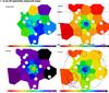 |
Fig. A.1 Two-dimensional X-ray spectrally measured temperature (upper left),
electron number-density (upper right), entropy (lower
left), and pressure (lower right) maps using the
Cappellari & Copin (2003) binning scheme. Overlaid circles in blue, red, and
green denote cluster galaxies that have spectroscopic follow-up data with their
clustercentric velocities toward the observer greater than 1000 km s-1,
away from the observer greater than 1000 km s-1, and smaller than
1000 km s-1, respectively. The radii of these circles are proportional to
|
Acknowledgments
We acknowledge our referee Andrea Biviano, who provided insight and expertise that greatly improved the work. Y.Y.Z. acknowledges Italo Balestra, Hans Böhringer, Angela Bongiorno, Paola Popesso, David Wilman, and Felicia Ziparo for useful discussions. Y.Y.Z. acknowledges support by the German BMBF through the Verbundforschung under grant 50 OR 1103. The XMM-Newton project is an ESA Science Mission with instruments and contributions directly funded by ESA Member States and the USA (NASA). The XMM-Newton project is supported by the Bundesministerium für Wirtschaft und Technologie/Deutsches Zentrum für Luft- und Raumfahrt (BMWI/DLR, FKZ 50 OX 0001) and the Max-Planck Society. We have made use of VLT/VIMOS observations taken with the ESO Telescope at the Paranal Observatory under programme 077.A-0058 and WFI observations partially supported by the Deutsche Forschungsgemeinschaft (DFG) through Transregional Collaborative Research Centre TRR 33. The VLT/VIMOS data presented in this paper were reduced using the VIMOS Interactive Pipeline and Graphical Interface (VIPGI) designed by the VIRMOS Consortium. This research has made use of the SIMBAD database, operated at CDS, Strasbourg, France.
References
- Andreon, S. 2010, MNRAS, 407, 263 [NASA ADS] [CrossRef] [Google Scholar]
- Arnal, E. M., Bajaja, E., Larrarte, J. J., et al. 2000, A&AS, 142, 35 [NASA ADS] [CrossRef] [EDP Sciences] [Google Scholar]
- Arnaud, M., Pointecouteau, E., & Pratt, G. W. 2005, A&A, 441, 893 [NASA ADS] [CrossRef] [EDP Sciences] [Google Scholar]
- Arnaud, M., Pointecouteau, E., & Pratt, G. W. 2007, A&A, 474, L37 [NASA ADS] [CrossRef] [EDP Sciences] [Google Scholar]
- Baade, D., Meisenheimer, K., Iwert, O., et al. 1999, The Messenger, 95, 15 [NASA ADS] [Google Scholar]
- Bajaja, E., Arnal, E. M., Larrarte, J. J., et al. 2005, A&A, 440, 767 [NASA ADS] [CrossRef] [EDP Sciences] [Google Scholar]
- Balogh, M. L., Navarro, J. F., & Morris, S. L. 2000, ApJ, 540, 113 [NASA ADS] [CrossRef] [Google Scholar]
- Bartelmann, M. 1996, A&A, 313, 697 [NASA ADS] [Google Scholar]
- Bauer, F. E., Condon, J. J., Thuan, T. X., & Broderick, J. J. 2000, ApJS, 129, 547 [NASA ADS] [CrossRef] [Google Scholar]
- Baum, W. A. 1959, PASP, 71, 106 [NASA ADS] [CrossRef] [Google Scholar]
- Becker, R. A., Chambers, J. M., & Wilks, A. R. 1988 (Pacific Grove, Ca.: Wadsworth Brooks) [Google Scholar]
- Beers, T. C., Flynn, K., & Gebhardt, K. 1990, AJ, 100, 32 [NASA ADS] [CrossRef] [Google Scholar]
- Bell, E. F., & de Jong, R. S. 2001, ApJ, 550, 212 [NASA ADS] [CrossRef] [Google Scholar]
- Bell, E. F., McIntosh, D. H., Katz, N., & Weinberg, M. D. 2003, ApJS, 149, 289 [NASA ADS] [CrossRef] [Google Scholar]
- Bertin, E., & Arnouts, S. 1996, A&AS, 117, 393 [NASA ADS] [CrossRef] [EDP Sciences] [Google Scholar]
- Biviano, A., & Salucci, P. 2006, A&A, 452, 75 [NASA ADS] [CrossRef] [EDP Sciences] [Google Scholar]
- Biviano, A., Murante, G., Borgani, S., et al. 2006, A&A, 456, 23 [NASA ADS] [CrossRef] [EDP Sciences] [Google Scholar]
- Böhringer, H., Schuecker, P., Guzzo, L., et al. 2001, A&A, 369, 826 [NASA ADS] [CrossRef] [EDP Sciences] [Google Scholar]
- Böhringer, H., Burwitz, V., Zhang, Y.-Y., Schuecker, P., & Nowak, N. 2005, ApJ, 633, 148 [NASA ADS] [CrossRef] [Google Scholar]
- Böhringer, H., Pratt, G. W., Arnaud, M., et al. 2010, A&A, 514, A32 [NASA ADS] [CrossRef] [EDP Sciences] [Google Scholar]
- Braglia, F., Pierini, D., & Böhringer, H. 2007, A&A, 470, 425 [NASA ADS] [CrossRef] [EDP Sciences] [Google Scholar]
- Butcher, H., & Oemler, A., Jr.1978, ApJ, 226, 559 [NASA ADS] [CrossRef] [Google Scholar]
- Cappellari, M., & Copin, Y. 2003, MNRAS, 342, 345 [NASA ADS] [CrossRef] [Google Scholar]
- Carlberg, R. G., Yee, H. K. C., Ellingson, E., et al. 1997, ApJ, 476, L7 [NASA ADS] [CrossRef] [Google Scholar]
- Christlein, D., & Zabludoff, A. I. 2003, ApJ, 591, 764 [NASA ADS] [CrossRef] [Google Scholar]
- Danese, L., de Zotti, G., & di Tullio, G. 1980, A&A, 82, 322 [NASA ADS] [Google Scholar]
- den Hartog, R., & Katgert, P. 1996, MNRAS, 279, 349 [NASA ADS] [CrossRef] [Google Scholar]
- Diaferio, A. 1999, MNRAS, 309, 610 [NASA ADS] [CrossRef] [Google Scholar]
- Diaferio, A., & Geller, M. J. 1997, ApJ, 481, 633 [NASA ADS] [CrossRef] [Google Scholar]
- Diehl, S., & Statler, T. S. 2006, MNRAS, 368, 497 [NASA ADS] [CrossRef] [Google Scholar]
- Dressler, A., & Shectman, S. A. 1988, AJ, 95, 985 [NASA ADS] [CrossRef] [Google Scholar]
- Durret, F., Laganá, T. F., & Haider, M. 2011, A&A, 529, A38 [NASA ADS] [CrossRef] [EDP Sciences] [Google Scholar]
- Erben, T., Schirmer, M., Dietrich, J. P., et al. 2005, Astron. Nachr., 326, 432 [NASA ADS] [CrossRef] [Google Scholar]
- Evrard, A. E., Bialek, J., Busha, M., et al. 2008, ApJ, 672, 122 [NASA ADS] [CrossRef] [Google Scholar]
- Fadda, D., Girardi, M., Giuricin, G., Mardirossian, F., & Mezzetti, M. 1996, ApJ, 473, 670 [NASA ADS] [CrossRef] [Google Scholar]
- Fujita, Y., & Nagashima, M. 1999, ApJ, 516, 619 [NASA ADS] [CrossRef] [Google Scholar]
- Garilli, B., Fumana, M., Franzetti, P., et al. 2010, PASP, 122, 827 [NASA ADS] [CrossRef] [Google Scholar]
- Geller, M. J., Diaferio, A., & Kurtz, M. J. 1999, ApJ, 517, L23 [NASA ADS] [CrossRef] [Google Scholar]
- Ghizzardi, S. 2001, in-flight calibration of the PSF for the MOS1 and MOS2 cameras, EPIC-MCT-TN-011, Internal Report [Google Scholar]
- Giacintucci, S., Markevitch, M., Brunetti, G., Cassano, R., & Venturi, T. 2011, A&A, 525, L10 [NASA ADS] [CrossRef] [EDP Sciences] [Google Scholar]
- Gill, S. P. D., Knebe, A., & Gibson, B. K. 2005, MNRAS, 356, 1327 [NASA ADS] [CrossRef] [Google Scholar]
- Girardi, M., Biviano, A., Giuricin, G., Mardirossian, F., & Mezzetti, M. 1993, ApJ, 404, 38 [NASA ADS] [CrossRef] [Google Scholar]
- Gladders, M. D., Lopez-Cruz, O., Yee, H. K. C., & Kodama, T. 1998, ApJ, 501, 571 [NASA ADS] [CrossRef] [Google Scholar]
- Gonzales, A. H., Zaritsky, D., & Zabludoff, A. I. 2007, ApJ, 666, 147 [NASA ADS] [CrossRef] [Google Scholar]
- Guo, F., & Mathews, W. G. 2010, ApJ, 712, 1311 [NASA ADS] [CrossRef] [Google Scholar]
- Hansen, S. M., McKay, T. A., Wechsler, R. H., et al. 2005, ApJ, 633, 122 [NASA ADS] [CrossRef] [Google Scholar]
- Hansen, S. M., Sheldon, E. S., Wechsler, R. H., & Koester, B. P. 2009, ApJ, 699, 1333 [NASA ADS] [CrossRef] [Google Scholar]
- Harrison, E. R., & Noonan, T. W. 1979, ApJ, 232, 18 [NASA ADS] [CrossRef] [Google Scholar]
- Hartmann, D., & Burton, W. B. 1997 (Cambridge University Press) [Google Scholar]
- Hildebrandt, H., Erben, T., Dietrich, J. P., et al. 2006, A&A, 452, 1121 [NASA ADS] [CrossRef] [EDP Sciences] [Google Scholar]
- Hou, A., Parker, L. C., Wilman, D. J., et al. 2012, MNRAS, 421, 3594 [NASA ADS] [CrossRef] [Google Scholar]
- Johnston, D. E., Sheldon, E. S., Wechsler, R. H., et al. 2007 [arXiv:0709.1159] [Google Scholar]
- Kaiser, N. 1987, MNRAS, 227, 1 [NASA ADS] [CrossRef] [Google Scholar]
- Kalberla, P. M. W., Burton, W. B., Hartmann, D., et al. 2005, A&A, 440, 775 [NASA ADS] [CrossRef] [EDP Sciences] [Google Scholar]
- Katgert, P., Mazure, A., Perea, J., et al. 1996, A&A, 310, 8 [NASA ADS] [Google Scholar]
- Katgert, P., Biviano, A., & Mazure, A. 2004, ApJ, 600, 657 [NASA ADS] [CrossRef] [Google Scholar]
- Kauffmann, G., Colberg, J. M., Diaferio, A., & White, S. D. M. 1999, MNRAS, 307, 529 [NASA ADS] [CrossRef] [Google Scholar]
- Lin, Y.-T., Mohr, J. J., & Stanford, S. A. 2004, ApJ, 610, 745 [NASA ADS] [CrossRef] [Google Scholar]
- Mahdavi, A., Hoekstra, H., Babul, A., & Henry, J. P. 2008, MNRAS, 384, 1567 [NASA ADS] [CrossRef] [Google Scholar]
- Markevitch, M., Forman, W. R., Sarazin, C. L., & Vikhlinin, A. 1998, ApJ, 503, 77 [NASA ADS] [CrossRef] [Google Scholar]
- Navarro, J. F., Frenk, C. S., & White, S. D. M. 1997, ApJ, 490, 493 [NASA ADS] [CrossRef] [Google Scholar]
- Odenkirchen, M., Grebel, E. K., Rockosi, C. M., et al. 2001, ApJ, 548, L165 [NASA ADS] [CrossRef] [Google Scholar]
- Ogrean, G. A., Hatch, N. A., Simionescu, A., et al. 2010, MNRAS, 406, 354 [NASA ADS] [CrossRef] [Google Scholar]
- Pisani, A. 1993, MNRAS, 265, 706 [NASA ADS] [Google Scholar]
- Pisani, A. 1996, MNRAS, 278, 697 [NASA ADS] [CrossRef] [Google Scholar]
- Poggianti, B. M., & Wu, H. 2000, ApJ, 529, 157 [NASA ADS] [CrossRef] [Google Scholar]
- Poole, G. B., Fardal, M. A., Babul, A., et al. 2006, MNRAS, 373, 881 [NASA ADS] [CrossRef] [Google Scholar]
- Popesso, P., Biviano, A., Böhringer, H., Romaniello, M., & Voges, W. 2005a, A&A, 433, 431 [NASA ADS] [CrossRef] [EDP Sciences] [Google Scholar]
- Popesso, P., Böhringer, H., Romaniello, M., & Voges, W. 2005b, A&A, 433, 415 [NASA ADS] [CrossRef] [EDP Sciences] [Google Scholar]
- Popesso, P., Biviano, A., Romaniello, M., & Böhringer, H. 2007, A&A, 461, 411 [NASA ADS] [CrossRef] [EDP Sciences] [Google Scholar]
- Pratt, G. W., Böhringer, H., Croston, J. H., et al. 2007, A&A, 461, 71 [NASA ADS] [CrossRef] [EDP Sciences] [Google Scholar]
- Quilis, V., Moore, B., & Bower, R. 2000, Science, 288, 1617 [NASA ADS] [CrossRef] [PubMed] [Google Scholar]
- Reyes, R., Mandelbaum, R., Hirata, C., Bahcall, N., & Seljak, U. 2008, MNRAS, 390, 1157 [NASA ADS] [CrossRef] [Google Scholar]
- Ricker, P. M., & Sarazin, C. L. 2001, ApJ, 561, 621 [NASA ADS] [CrossRef] [Google Scholar]
- Rines, K., & Diaferio, A. 2006, ApJ, 132, 1275 [Google Scholar]
- Roettiger, K., Burns, J. O., & Stone, J. M. 1999, ApJ, 518, 603 [NASA ADS] [CrossRef] [Google Scholar]
- Saintonge, A., Tran, K.-V. H., & Holden, B. P. 2008, ApJ, 685, L113 [NASA ADS] [CrossRef] [Google Scholar]
- Salpeter, E. E. 1955, ApJ, 121, 161 [Google Scholar]
- Sanders, J. S. 2006, MNRAS, 371, 829 [NASA ADS] [CrossRef] [Google Scholar]
- Schechter, P. 1976, ApJ, 203, 297 [Google Scholar]
- Scodeggio, M., Franzetti, P., Garilli, B., et al. 2005, PASP, 117, 1284 [NASA ADS] [CrossRef] [Google Scholar]
- Snowden, S. L., Mushotzky, R. F., Kuntz, K. D., & Davis, D. S. 2008, A&A, 478, 615 [NASA ADS] [CrossRef] [EDP Sciences] [Google Scholar]
- Sun, M., Donahue, M., & Voit, G. M. 2007, ApJ, 671, 190 [NASA ADS] [CrossRef] [Google Scholar]
- Urquhart, S. A., Willis, J. P., Hoekstra, H., & Pierre, M. 2010, MNRAS, 406, 368 [NASA ADS] [CrossRef] [Google Scholar]
- Verdugo, M., Ziegler, B. L., & Gerken, B. 2008, A&A, 486, 9 [NASA ADS] [CrossRef] [EDP Sciences] [Google Scholar]
- Verdugo, M., Lerchster, M., Böhringer, H., et al. 2012, MNRAS, 421, 1949 [NASA ADS] [CrossRef] [Google Scholar]
- Vikhlinin, A., Kravtsov, A., Forman, W., et al. 2006, ApJ, 640, 691 [NASA ADS] [CrossRef] [Google Scholar]
- Zhang, Y.-Y., Böhringer, H., Finoguenov, A., et al. 2006, A&A, 456, 55 [NASA ADS] [CrossRef] [EDP Sciences] [Google Scholar]
- Zhang, Y.-Y., Finoguenov, A., Böhringer, H., et al. 2007, A&A, 467, 437 [NASA ADS] [CrossRef] [EDP Sciences] [Google Scholar]
- Zhang, Y.-Y., Finoguenov, A., Böhringer, H., et al. 2008, A&A, 482, 451 [NASA ADS] [CrossRef] [EDP Sciences] [Google Scholar]
- Zhang, Y.-Y., Reiprich, T. H., Finoguenov, A., Hudson, D. S., & Sarazin, C. L. 2009, ApJ, 699, 1178 [NASA ADS] [CrossRef] [Google Scholar]
- Zhang, Y.-Y., Okabe, N., Finoguenov, A., et al. 2010, ApJ, 711, 1033 [NASA ADS] [CrossRef] [Google Scholar]
- Zhang, Y.-Y., Andernach, H., Caretta, C. A., et al. 2011a, A&A, 526, A105 [NASA ADS] [CrossRef] [EDP Sciences] [Google Scholar]
- Zhang, Y.-Y., Laganá, T. F., Pierini, D., et al. 2011b, A&A, 535, A78 [NASA ADS] [CrossRef] [EDP Sciences] [Google Scholar]
- Zibetti, S., White, S. D. M., Schneider, D. P., & Brinkmann, J. 2005, MNRAS, 358, 949 [Google Scholar]
- Ziparo, F., Braglia, F. G., Pierini, D., et al. 2012, MNRAS, 420, 2480 [NASA ADS] [CrossRef] [Google Scholar]
All Tables
All Figures
|
Fig. 1 MOS1 (black), MOS2 (red), and pn (green) spectra extracted from the central
≤ 0 |
| In the text | |
|
Fig. 2 Left: deprojected temperature measurement versus radius with the
parametrized temperature distribution indicated by the solid curve and the
1σ interval by the dashed curves. The vertical line denotes
|
| In the text | |
|
Fig. 3 Cumulative mass distributions (1) using the X-ray hydrostatic method (filled
squares), (2) using the caustic method (black solid curve), (3) of the gas mass
estimate (black dotted curve), (4) of the stellar mass estimate of the red galaxies
(red dash-dotted curve), and (5) of the stellar mass estimate of the blue galaxies
(blue dash-dotted-dotted-dotted curve). The dashed curves and error bars denote
1σ intervals. The open star, triangle, diamond, and circle
indicate the dynamical mass estimates ( |
| In the text | |
|
Fig. 4 Two-dimensional X-ray spectrally measured temperature (upper
left), electron number-density (upper right), entropy
(lower left), and pressure (lower right) maps
using the Sanders (2006) binning scheme.
Overlaid circles in blue, red, and green denote cluster galaxies that have
spectroscopic follow-up data with their clustercentric velocities toward the
observer greater than 1000 km s-1, away from the observer greater than
1000 km s-1, and smaller than 1000 km s-1, respectively. The
radii of these circles are proportional to |
| In the text | |
|
Fig. 5 Temperature (upper left), electron number-density (upper right), entropy (lower left), and pressure (lower right) distributions of the spectrally measured 2D maps using the Sanders (2006) binning scheme are shown as crosses with their local regression fits in black curves. The solid and dashed grey curves in the upper left plot show the parametrization of the deprojected temperature profile and its 1-σ interval derived in Sect. 2.3. Differential scatter and its 1-σ intervals of the temperature, electron number-density, entropy, and pressure fluctuations in the 2D maps are shown in solid and dashed black curves in their upper panels. |
| In the text | |
|
Fig. 6 Radial distribution of the iron abundance. The vertical line
denotes |
| In the text | |
|
Fig. 7 Left: histogram of the line-of-sight velocities. Member galaxies
of the cluster, member galaxies of the high velocity group, and non-member galaxies
are in solid (black), dashed (red), and dash-dotted (grey) lines. The arrow shows
the cluster redshift. Right: line-of-sight velocity versus
projected radius, in which filled blue diamonds and red stars show blue and red
member galaxies in the caustic (black curve), and open squares show fore- and
background galaxies. The grey curve shows the symmetric boundary by choosing the
minimum of the values on both sides of the caustic boundary relative to the cluster
redshift. The cluster radii, |
| In the text | |
|
Fig. 8 WFI B-band imaging. Overlaid circles in blue, red and green denote
cluster galaxies with spectroscopic follow-up data that have clustercentric
velocities toward the observer greater than 1000 km s-1, away from the
observer greater than 1000 km s-1, and smaller than
1000 km s-1, respectively. The radii of these circles are proportional
to |
| In the text | |
|
Fig. 9 Left: colour–magnitude diagram with the corresponding red sequence
indicated by a solid line and its 3σ = 0.249 magnitude intervals by
dashed lines. The sample is complete down to the curve at ~22 mag, which varies
slightly with the B − R colour. We thus limited
the analysis to the galaxies brighter than R = 22 mag. The dotted
line denotes the colour cut that is 1.5 mag bluer than the red sequence, below which
the objects were considered as foreground contamination. Red stars and blue diamonds
indicate red and blue spectroscopic member galaxies regardless of their
clustercentric distances. The BCG is extremely blue with
B − R = 0.98. Right: cluster
galaxy luminosity functions for red (red stars), blue (blue diamonds), and all
(black circles) members within |
| In the text | |
|
Fig. 10 Left: number density profiles with their best-fit NFW models for
red member galaxies (red triangles, solid curve) and all members (black circles,
dashed curve), respectively. We obtained reduced
χ2 = 1.03,2.24 for the red and all
member galaxies, which indicates that the red galaxies follow well the theoretical
profile and the blue galaxies may account for the deviation of the fit for all
member galaxies. The bin size is 300 kpc. Right: ratio of blue to
all member galaxies as a function of projection distance from the X-ray
flux-weighted centroid. The vertical line
remarks |
| In the text | |
|
Fig. A.1 Two-dimensional X-ray spectrally measured temperature (upper left),
electron number-density (upper right), entropy (lower
left), and pressure (lower right) maps using the
Cappellari & Copin (2003) binning scheme. Overlaid circles in blue, red, and
green denote cluster galaxies that have spectroscopic follow-up data with their
clustercentric velocities toward the observer greater than 1000 km s-1,
away from the observer greater than 1000 km s-1, and smaller than
1000 km s-1, respectively. The radii of these circles are proportional to
|
| In the text | |
Current usage metrics show cumulative count of Article Views (full-text article views including HTML views, PDF and ePub downloads, according to the available data) and Abstracts Views on Vision4Press platform.
Data correspond to usage on the plateform after 2015. The current usage metrics is available 48-96 hours after online publication and is updated daily on week days.
Initial download of the metrics may take a while.