| Issue |
A&A
Volume 542, June 2012
|
|
|---|---|---|
| Article Number | A112 | |
| Number of page(s) | 14 | |
| Section | The Sun | |
| DOI | https://doi.org/10.1051/0004-6361/201218887 | |
| Published online | 19 June 2012 | |
An active region filament studied simultaneously in the chromosphere and photosphere
II. Doppler velocities⋆
1 Instituto de Astrofísica de Canarias, vía Láctea s/n, 38205 La Laguna, Tenerife, Spain
e-mail: This email address is being protected from spambots. You need JavaScript enabled to view it.
2 Departamento de Astrofísica, Universidad de La Laguna, 38206 La Laguna, Tenerife, Spain
3 High Altitude Observatory (NCAR), Boulder, CO 80301, USA
Received: 25 January 2012
Accepted: 20 April 2012
Abstract
Context. Paper I presents the magnetic structure, inferred for the photosphere and the chromosphere, of a filament that developed in active region (AR) NOAA 10781, observed on 2005 July 3 and July 5.
Aims. In this paper we complement those results with the velocities retrieved from Doppler shifts measured at the chromosphere and the photosphere in the AR filament area.
Methods. The velocities and magnetic field parameters were inferred from full Stokes inversions of the photospheric Si i 10 827 Å line and the chromospheric He i 10 830 Å triplet. Various inversion methods with different numbers of atmospheric components and different weighting schemes of the Stokes profiles were used. The velocities were calibrated on an absolute scale.
Results. A ubiquitous chromospheric downflow is found in the faculae surrounding the filament, with an average velocity of 1.6 km s-1. The filament region, however, displays upflows in the photosphere on both days, when the linear polarization (which samples the transverse component of the fields) is given more weight in the inversions. The upflow speeds of the transverse fields in the filament region average −0.15 km s-1. In the chromosphere, the situation is different for the two days of observation. On July 3, the chromospheric portion of the filament is moving upward as a whole with a mean speed of −0.24 km s-1. However, on July 5 only the section above an orphan penumbra shows localized upflow patches, while the rest of the filament is dominated by the same downflows observed elsewhere in the facular region. Photospheric supersonic downflows that last for tens of minutes are detected below the filament, close to the PIL.
Conclusions. The observed velocity pattern in this AR filament strongly suggests a scenario where the transverse fields are mostly dominated by upflows. The filament flux rope is seen to be emerging at all places and both heights, with a few exceptions in the chromosphere. This happens within a surrounding facular region that displays a generalized downflow in the chromosphere and localized downflows of supersonic character at the photosphere. No large scale downflow of transverse field lines is observed at the photosphere.
Key words: Sun: filaments, prominences / Sun: faculae, plages / Sun: photosphere / Sun: chromosphere / techniques: polarimetric
Appendices A and B are available in electronic form at http://www.aanda.org
© ESO, 2012
1. Introduction
Velocity measurements in active region (AR) filaments are extremely scarce in the literature. Most studies have been carried out only in quiescent (QS) filaments (outside ARs). However, quantifying velocities and plasma flows in filaments is a fundamental step toward understanding their formation, evolution and disappearance. Filaments are structures formed from cool dense plasma that typically lies between opposite polarities, i.e., at the polarity inversion line (PIL; Babcock & Babcock 1955), in the chromosphere or corona. Due to the temperature contrast with their surroundings, they appear as dark structures when observed on the solar disk. Filaments are called prominences if observed in emission above the limb, but both terms are often used interchangeably in the literature.
To date, there are two proposed scenarios for the formation process of filaments: the sheared arcade (SA) model and the flux rope emergence (FRE) model. Both result in very similar global structures, i.e., a flux rope that hangs above the photosphere (although the SA model combines dipped field lines and flux ropes). However, it is in the formation process of the flux ropes where the two models differ. The SA model requires shearing motions of the footpoints to form the flux rope in the corona with the aid of reconnection processes identified in the photosphere as cancellation events. On the other hand, in the FRE model the flux rope is formed deep in the convection zone (CZ) before it emerges through the surface and makes its way up into the corona. However, simulations based on buoyancy instabilities encounter difficulties when lifting up a mass-loaded flux rope from the photosphere into the corona (e.g., Murray et al. 2006; MacTaggart & Hood 2010). Kuckein et al. (2012, hereafter Paper I) provide a more thorough discussion and additional references to these two models (see also the extensive review by Mackay et al. 2010).
Nowadays, high-resolution imaging has shown that quiescent filaments are made of smaller-scale structures (e.g., Demoulin et al. 1987; Lin et al. 2005, and references therein). Doppler measurements in these quiescent filaments (e.g., Martres et al. 1981; Schmieder et al. 2010) have revealed that a wide range of velocities coexist in the same structure. For example, the recent study by Chae et al. (2007) reported line-of-sight (LOS) velocities between ±5 km s-1 and ± 15 km s-1 in the spine and in threads (respectively) of a QS filament (at coordinates N15-E26). Mein (1977) found that the axis of an AR filament (at N7-W30) was at rest, while downflows on one side and upflows on the other side were detected. Upward motions have also been detected below QS and AR filaments by Ioshpa & Obridko (1999). However, the main limitation of Doppler line shifts, and hence of the retrieved LOS velocities, is that the inferred values are position-dependent all over the solar disk. Therefore, it is hard to compare Doppler velocities measured in different filaments. In addition, a thorough calibration, i.e., setting a correct zero value for the rest wavelength, is necessary, especially when calculating photospheric velocities (below the filament) which are much smaller (≤0.3 km s-1; Martres et al. 1976) than those found in the chromosphere and corona (see Welsch & Fisher 2012).
It is presently unclear whether there is an unequivocal way of distinguishing which of the different filament formation scenarios applies to the observed AR filament. In this paper we propose to shed some light on this topic by studying the observed Doppler velocities inside the AR filament that was analyzed in Paper I. In particular, we can ask what the expected velocity patterns (in and below the filaments) associated with these two models are. The flux rope models proposed by van Ballegooijen & Martens (1989) and van Ballegooijen & Mackay (2007) are built through successive photospheric flux cancellations driven by motions that force the field lines to converge toward the PIL. After the oppositely directed field lines are brought together, reconnection processes above the photosphere create a flux rope in the corona. The authors suggest that transverse magnetic field lines (loops which are almost perpendicular to the PIL) submerge at the PIL, and are transported downward into the CZ as a result of the reconnection processes mentioned before (see panels d and e in Fig. 1 of van Ballegooijen & Martens 1989). The typical size of these submerging loops is small (~900 km), which is large enough to be detected with currently available instruments.
The prominence model presented in the work of DeVore & Antiochos (2000) does not show convergence of flux at the PIL. The helicity in the field lines is built up in the corona as a consequence of reconnection of the highly sheared field lines (twisted and stretched by the sheared displacements of the footpoints) with the overlying coronal arcade. The authors point out that the resulting magnetic structure is stable; hence, no upflows or downflows are expected in this model. However, the observed evolution of filaments suggests that they are of a non-steady nature. This calls for models with built-in evolutionary processes that allow the filament to disappear from the solar surface, transporting magnetic fields upward or downward through the photospheric boundary.
The first complete description of the emergence of a flux rope AR filament was presented by Okamoto et al. (2008, 2009). The authors show observational evidence of an emerging helical flux rope that apparently reconnects with the remnant magnetic field of a pre-existing filament. A Milne-Eddington (ME) inversion of the Stokes profiles observed with Hinode/SP over the region where the transverse fields of the emerging flux rope were observed yielded a mean upflow of − 0.3 ± 0.2 km s-1. The ME inversion applied by these authors was able to separate the velocity of the magnetic and the non-magnetic components (see their Fig. 2). Interestingly, while the non-magnetic atmosphere showed a typical granulation pattern, upflows were systematically inferred for the magnetic component. Thus, in that work, the picture of the filament formation is compatible with the existence of transverse fields that are moving upward into the chromosphere and corona. MacTaggart & Hood (2010) simulated the rise of a weakly twisted flux tube from the solar interior up into an overlying arcade in the corona. The axis of their flux rope became trapped slightly above the photosphere, while the field lines of the top of the flux rope were still able to reach coronal heights. In the same way, the 3D MHD simulations of an emerging flux rope presented by Yelles Chaouche et al. (2009) showed horizontal field lines that moved upward with velocities of ~−0.67 km s-1. However, the authors pointed out that the emergent flux studied by Okamoto et al. (2009) was probably less buoyant than the case simulated in their work, since the observed rising speed was smaller and the modification of the granular pattern less severe than in the simulations. Interestingly, Lites et al. (2010) also found a similar pattern to that presented by Okamoto et al. (2009) in their study of the evolution of a filament channel inside an AR. The inferred magnetic structure in the filament channel corresponded to horizontal field lines elongated along the PIL (with equipartition strengths) that often (but not always) displayed upflows (see the vmag panel in Fig. 5 of Lites et al. 2010). A slow continuous upward motion in active region filaments had already been observed almost three decades ago (Malherbe et al. 1983; Schmieder et al. 1985), albeit in chromospheric layers. It is thus clear that studying the behavior of transverse magnetic fields at the location of filaments (i.e., at AR PILs), is crucial to understanding their evolution (see also the discussion in Welsch & Fisher 2012). In particular, it will help to shed some light on how the magnetic structures that sustain the filaments get filled with plasma and how they eventually get rid of it, unloading most of their mass. To this end, it is crucial to obtain more data of the flows associated with filament formation and evolution.
In Paper I, we presented the magnetic structure of an AR filament, inferred from simultaneous spectropolarimetric observations in the photosphere and chromosphere. The filament seemed to be divided into two parts: (1) one section that showed a flux rope configuration which had its main axis lying in the chromosphere; and (2) another section, which was likely to have a similar magnetic structure, but whose main axis was detected in the photosphere instead. This extremely low-lying part of the filament left an imprint on the photosphere in the shape of an orphan penumbral system in the proximity of small pore associations. Paper I suggested that these features were the photospheric counterpart of the filament. However, in order to understand the formation mechanism of this AR filament, a detailed study of the Doppler velocities, in a global scenario, needs to be carried out. The present paper addresses this issue by focusing in particular on the photospheric velocities inferred from the Doppler shifts of the Si i line in order to search for systematic upflows and downflows. We also analyze the chromospheric Doppler shifts provided by the He i triplet.
2. Observations
The AR under study, NOAA AR 10781, was in its slow decay phase during our observing run in July 2005. The AR had a round leader sunspot of positive polarity and was followed by an extensive plage region that stretched toward higher latitudes. On top of the PIL, a filament with an inverse S-shape was unambiguously identified. Two spectropolarimetric maps were taken on July 3 (at latitude and longitude N16-E8, μ ~ 0.95), and seven on July 5 (at N16-W18, μ ~ 0.91), using the Tenerife Infrared Polarimeter (TIP-II; Collados et al. 2007) at the German Vacuum Tower Telescope (VTT) on Tenerife. In addition, a time series of ~19 min, with the slit fixed at the PIL, was acquired on July 5.
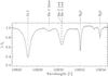 |
Fig. 1 Stokes I profile, normalized to the continuum intensity, observed by TIP-II near the PIL. The dashed vertical lines indicate the positions of the rest wavelengths for the spectral lines that are used in this work. |
Atomic data used in this work.
The slit (0 5 wide and 35′′ long, with a pixel size of 017 along the slit) was aligned with the filament and a series of spectropolarimetric maps, centered on the filament, were acquired using a scanning step size of 04 or 03, depending on the seeing conditions. Figure 1 shows the spectral range of the spectropolarimeter, which comprises the photospheric Si i 10 827 Å line, the chromospheric He i 10 830 Å triplet and two telluric H2O lines. The helium triplet comprises a “blue” component and two blended “red” components. Table 1 provides the wavelength and the logarithm of the oscillator strength times the multiplicity of the lower level, log gf, for each line. This unique spectral window allows us to study the photosphere and the chromosphere simultaneously. The seeing conditions during the observations were highly variable and the adaptive optics system of the VTT (KAOS; von der Lühe et al. 2003) helped to substantially improve the image quality. The data sets were corrected for flat field, dark current and polarimetric calibration using the standard procedures for TIP (Collados 1999, 2003).
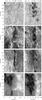 |
Fig. 2 TIP-II slit-reconstructed images for both days of observation. From top to bottom: continuum, Si i line core intensity, He i line core intensity (red component) and Si i Stokes V. The FOV was different on July 3 and July 5. We provide the dashed rectangles to show the approximate common area of the filament on both days. Characters a) − d) indicate the position of the Stokes profiles presented in Fig. 7. The white arrows point to high concentrations of helium with elongated shapes (thread-like structures). |
Figure 2 shows an example, for both days, of the scanned area of the filament. From top to bottom, the slit-reconstructed images presented correspond to different wavelength bands: continuum intensity, Si i line core intensity, He i line core intensity centered at the red component and Si i LOS magnetogram. On July 3, the filament had a thin elongated shape in the chromosphere (see He i panel of Fig. 2), which we interpret to be the main axis or spine of the filament. Underneath, in the photosphere, the continuum image shows no outstanding features. The field-of-view (FOV) of July 5 was slightly different and included newly appearing pores and orphan penumbral structures in the photosphere, mainly located along the PIL and below the filament (see continuum image in the top righthand panel). The white dashed rectangles in Fig. 2 show the approximate portion of the filament common to both days of observation. The He i intensity image of July 5 also shows the spine of the filament in the lower (common) part of the FOV. This feature is traced by an elongated shape in the Si i line core image, indicating that the structure lies at a lower mean height than on July 3. In the upper part of the He i image, on the other hand, the filament is more diffuse and less compact, and shows a series of dark threads that are highlighted by the white arrows (see also Fig. 5 of Paper I for more TIP-II images from July 5). Since the structure of the filament is identifiable in the silicon images, Paper I concluded that the filament was extremely low-lying and was directly responsible for the orphan penumbral aggregations and pores.
The main purpose of this paper is to identify what the plasma motions associated with the filament are, both in the chromosphere and the photosphere. In particular, we concentrate on whether the field lines are moving upward, which would indicate an emerging process, or downward, which would reveal a submergence phenomenon. The position on the solar disk of this AR is quite close to disk center on both days. This presents an advantage for the study of LOS velocities, which should not differ too much from the vertical velocities (measured in a local solar reference frame). For a better understanding of the inferred velocities we will distinguish between two regions in the filament: the spine area and the diffused filament area (above the orphan penumbrae), the latter being observed only on July 5. As stated in Paper I, these two areas correspond to the same filament, but observed at different heights. It is therefore helpful to study them separately.
A detailed analysis of the evolution of this AR was presented in Paper I.
3. Data analysis
To infer the physical parameters from the available sets of spectropolarimetric data we used two different inversion codes. It is important to recall that an inversion code provides full vector magnetic fields, but only the LOS component of the velocity, in the observer’s reference frame. Since one infers the three components of the vector magnetic field, the resulting inclinations and azimuths can be projected onto the local solar reference frame (i.e., with respect to the solar vertical, z, and along the solar latitude and longitude planes). However, difficulties arise when this transformation is carried out. The well-known 180° ambiguity (due to the angular dependence of Stokes Q and U with the azimuth) provides two solutions for the magnetic field, with different azimuths and inclinations when projected onto the local solar reference frame. To find the correct solution, we used the AZAM code for the disambiguation of the magnetic field vector (Lites et al. 1995) (see also Sect. 3.2 of Paper I for a more detailed explanation). Doppler shifts provide only one component of the velocity vector, the one projected along the LOS, rendering the projection onto the local solar frame impossible. Since the aim of this work is to compare the LOS velocities and their associated vector magnetic fields, for the remainder of this paper we will leave the magnetic field inclinations and azimuths in the observer’s frame. As our observations were done relatively close to disk center, the distinction between the two frames is more quantitative than qualitative. In order to show the impact of using the vector magnetic field in the observer’s frame instead of in the local solar frame, Table 2 provides two examples of the inclinations (γ → γ⊙) and the azimuths (φ → φ⊙), averaged over several pixels, in both reference frames. An inclination of γ = 90° in the LOS frame means that the field lines are perpendicular to the LOS, while γ⊙ = 90° means that they are parallel to the solar surface. As can be deduced from Table 2, while the exact values differ between the two frames, the horizontal or vertical nature of the field vectors is mostly preserved.
Examples of the LOS to local solar reference frame transformation of the magnetic field inclination and azimuth.
3.1. Helium 10 830 Å and silicon 10 827 Å inversions
Before inverting the helium spectra we carried out a 3 × 6 binning of the data along the scanning and slit directions, respectively, and a binning of 3 pixels in the spectral domain to increase the signal-to-noise ratio (S/N), rendering a value of ~2000 for all maps. The resulting spectral sampling is ~33.1 mÅ px-1 and the pixel size 1.2 × 1.0 arcsec2 and 1 × 1 arcsec2, for July 3 and 5, respectively. However, since the Si i line is much stronger than the He i triplet, the inversions of the former were carried out without any binning, the pixel size being 0.40 × 0.17 arcsec2 and 0.30 × 0.17 arcsec2, on July 3 and 5 respectively. This preserved the original spatial resolution at an expense of a lower S/N of ~500. The binned silicon data and inversions were used solely for the purpose of Table 2.
The chromospheric He i 10 830 Å triplet was inverted using a Milne-Eddington inversion code (MELANIE; Socas-Navarro 2001). This code assumes that the source function varies linearly with optical depth while the remaining semi-empirical parameters stay constant with height. MELANIE computes the Zeeman-induced Stokes profiles in the incomplete Paschen-Back (IPB) effect regime (see Socas-Navarro et al. 2004; Sasso et al. 2006, for a better understanding of the IPB effect on the Stokes profiles in the He i 10 830 Å region) and has a set of nine free parameters, which are iteratively modified by the code in order to obtain the best match between the synthetic and the observed Stokes data. The macroturbulence and the filling factor, or fraction of the magnetic component occupied inside each pixel, were fixed at 1.2 km s-1 and f = 1 in the inversion, so no stray-light was used. Atomic-level polarization is not taken into account in MELANIE. However, this is not necessary for this AR filament, since Kuckein et al. (2009) proved that these He i Stokes profiles are dominated by the Zeeman effect.
The photospheric Si i 10 827 Å line was inverted with the SIR code (Stokes Inversions based on Response functions; Ruiz Cobo & del Toro Iniesta 1992) which solves the radiative transfer equation assuming local thermodynamic equilibrium (LTE). SIR gives a depth-dependent stratification of the inferred physical parameter as a function of the logarithm of the LOS continuum optical depth at 5000 Å.
We carried out two sets of inversions for the Si i line. The first set, referred to hereafter as “standard” inversions, used a uniform weighting scheme for the four Stokes parameters: wI,Q,U,V = 1. An average intensity profile of the non-magnetic areas of each map (regions where Stokes Q, U, and V had negligible values), was used as representative of the stray-light. The stray-light fraction, α, used here as a proxy for the filling factor, was left as a free parameter in the inversion. Note that in the case of helium, the line is weak in quiet regions, so the use of a magnetic filling factor does not provide any benefit. We studied the response function (RF) to velocity perturbations in several model atmospheres obtained from the inversion of the filament data, finding a consistent value of log τ = −2 for the height at which the sensitivity was the highest. The height stratification derived by the inversion code was not used since the velocities at other optical depths had larger error bars.
The Doppler shift of the stray-light profile cannot be set as a free parameter in the SIR inversion code. This extra freedom was used in the studies by Okamoto et al. (2009) and Lites et al. (2010) to separate the magnetic and non-magnetic Doppler shifts. While the latter were dominated by granulation patterns, the former provided clear indications of upflows – a crucial result that we want to investigate further in this paper. To this end, we produced a second set of SIR inversions that were able to retrieve the Doppler shifts of the magnetic component without interference from a possible shift of the stray-light profile. These inversions, referred to heretofore as the “magnetic” inversions, forced a zero-weighting (wI = 0) for Stokes I, basically eliminating any sensitivity to the intensity profile, and hence to the stray-light, in the inversion procedure. Furthermore, since we were interested in the Doppler shifts of the transverse fields near the PIL, we weighted Stokes Q and U equally with wQ,U = 1 and set the weight of Stokes V to wV = 0.1. The filling factor was fixed to f = 1. The remaining parameters were initialized in the same way as in the “standard” silicon inversions.
Bard & Carlsson (2008) reported in their work that the Si i 10 827 Å line is formed in non local thermodynamic equilibrium (NLTE) conditions. In Paper I we tested the NLTE effects on the inversions of the Si i line in the filament, using the departure coefficients, β (defined as the ratio between the population densities calculated in NLTE and LTE), reported in Bard & Carlsson (2008). We found almost negligible changes in the retrieved LOS velocities, temperature being the only parameter that was substantially affected in the upper layers. Therefore, we decided not to consider the departure coefficients for the purpose of the present work.
The reader is referred to Paper I for a more thorough description of the inversions and NLTE effects.
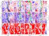 |
Fig. 3 LOS velocities inferred from: the Si i 10 827 Å full Stokes “standard” inversions (top row), the Si i 10 827 Å “magnetic” inversions (with weights: wI = 0, wQ,U = 1.0 and wV = 0.1) (middle row) and He i 10 830 Å inversions (bottom row) at different times. Note that the color scale is saturated at [−1, 1] and [−2, 2] km s-1 for silicon and helium respectively. Pixels inside the contours have magnetic field inclinations, with respect to the LOS, between 75° ≤ γ ≤ 105°. In the July 5 maps, the colored contours distinguish between the orphan penumbrae area (green) and the spine region (black). On July 3, only the spine of the filament was seen. Negative velocities (blue) indicate upflows while positive velocities (red) indicate downflows. |
3.1.1. Two-component inversions
The presence of several atypical Stokes V profiles (i.e., with several highly redshifted lobes) in the Si i 10 827 Å line led us to use a two-magnetic component SIR inversion for these cases (see Sect. 4.2). Therefore, we had two initial guess atmospheres. For the first one, we used the same atmospheric model as that from the previous single-component inversion, but for the second, we increased the magnetic field strength from 500 to 1500 Gauss and the velocity from 0.5 to 10 km s-1. These initial conditions resulted in a good performance of the SIR code.
3.2. Wavelength calibration
The main aim of this work is to provide reliable Doppler velocities measured at the filament at both heights. In order to calibrate these velocities on an absolute scale, we had to correct them for several effects such as Earth’s orbital motions and the solar gravitational redshift (see Appendix A for a complete description of the calibration). The wavelengths presented in Table 1 were all obtained from the National Institute of Standards and Technology (NIST) except for the one corresponding to the telluric line. The literature reports several values, with differences on the order of tens of mÅ, which are large enough to cause systematic errors in our velocity calibration. We propose a new value for the rest wavelength of this telluric line, which we inferred by calibrating flat field TIP-II data taken at disk center (see Appendix B).
4. Results
4.1. Doppler velocities
Mean Doppler velocities ( ⟨ v ⟩ ), of all available maps for both days, calculated inside the contours, where the inferred LOS inclinations are between 75° < γ < 105°, i.e., along the PIL.
The inferred LOS velocities of four representative cases (one on July 3 and three on July 5) are shown as slit-reconstructed maps in Fig. 3. Blue means upflow (v < 0) while red indicates downflow (v > 0). The pixels enclosed by the contours have LOS magnetic field inclinations between 75° ≤ γ ≤ 105°, γ being the inclination inferred from the corresponding silicon or helium inversions. This criterion was chosen to study the velocities associated to transverse fields which, as reported in Paper I, dominate along the filament. The contours denote the area they belong to. The green contours enclose pixels with transverse field lines which lay at the orphan penumbral region whereas the black contours correspond to the spine region. Bear in mind that the FOV on July 5 only overlaps approximately with the upper half of the July 3 map (the white dashed rectangles in Fig. 2 give an idea of the common FOV). Moreover, small shifts of the FOV (in the vertical direction) between different maps of July 5 are also present.
The panels in the upper row of Fig. 3 correspond to the Si i 10 827 Å velocities, scaled between ± 1 km s-1, inferred from the standard inversions, i.e., those with wI,Q,U,V = 1. We found alternating blue and red patches in all panels, which revealed a mixture of upflows and downflows along the PIL, i.e., inside the contours. However, it is clear that on July 3, the inside of the black contour is more dominated by upflows than on July 5. On this day, there are no significant differences between the velocity patterns of the orphan penumbrae and the spine.
We now turn to the panels of the middle row of Fig. 3. The velocity maps correspond to the magnetic inversions as defined in Sect. 3.1 (wI,Q,U,V = 0,1,1,0.1). We therefore assume that the velocities in these panels are more likely to represent the motions of the transverse magnetic field lines (as opposed to the maps from the first row, which are more influenced by unmagnetized regions and flows along vertical field lines). The inversion code had problems in converging properly when Stokes Q and U were small, i.e., where the magnetic fields were weak or almost vertical. Nevertheless, along the PIL, the inversion code performed well and the uncertainties obtained were on the same order of magnitude as those from the standard inversions. On July 5, a comparison of the middle with the upper panels reveals that the “magnetic” Si i velocities inside the contours are globally more dominated by blueshifts, rather than redshifts. We interpret this result as an indication of a predominant upward motion of the transverse field lines in the photosphere, in particular inside the orphan penumbrae (green contours). Similarly, on July 3, there is more of an upward trend in the motions of the transverse fields.
The velocity maps inferred from the (binned) He i 10 830 Å inversions are presented in the lower row of Fig. 3. Note that the color is now scaled between ± 2 km s-1. The first striking result are the ubiquitous red areas (indicative of downflows) that extend almost everywhere, with the exception of the region near the PIL. On July 3, an almost perfect correlation between the transverse field lines inferred from the helium inversions and the upflow areas can be seen within the black contour in the lower lefthand panel. Bearing in mind that on July 3 we clearly saw the filament axis in the helium core absorption map (see Fig. 2), and in Paper I we found sheared field lines parallel to its axis, one can easily deduce that the filament axis is rising in the chromosphere. Typical rising speeds are in the range [0, − 1.5] km s-1.
Two days later, on July 5, the spine region (black contours) hardly shows any upflows. The large-scale redshifted pattern seen elsewhere is, however, weaker. This means that, even if the filament axis was not moving upward on July 5, it was still able to interfere with the mechanism that generates the large scale downflows (see Sect. 4.3). In the diffuse filament region (above the orphan penumbrae, marked with green contours), the velocity pattern is fundamentally different. Once again, the transverse fields near the PIL harbor clear signs of upflows. It is thus evident that, while the general trend observed in He i corresponds to a large scale downflow, the filament axis (near the PIL) is a place where the downflows are not as strong and sporadic upflow patches are also present. We will discuss this issue later, in Sect. 4.3.
To understand the general trends in the velocity maps of Fig. 3, a statistical study of the average velocities ( ⟨ v ⟩ ) inside the black and green contours was carried out and compiled in Table 3. The number of averaged points (#) and the standard deviation (σ) are also provided in this table. We have found the following:
-
1.
On July 3, the mean velocities inferred from the Si i inversions at the spine (i.e., below the filament axis) show an obvious blueshift. The magnetic inversions, averaging
 ~ −0.150 km s-1, are more blueshifted than the standard inversions. Upflows are also found in the chromosphere ( ⟨ vHe ⟩ ~ − 0.240 km s-1).
 -
2.
For the first four maps of July 5, the spine presents an upward motion of the photospheric transverse fields (black contours) as inferred from the magnetic inversions, with typical velocities of
= − 0.215 km s-1. In the last three maps the velocities drop to almost zero. The standard Si i inversions show, by contrast, velocities which oscillate around zero ( ⟨ vSi ⟩ ~ − 0.012 km s-1). -
3.
On July 5, the chromospheric velocities at the spine are dominated by downflows in the range of vHe ∈ [0.65,1.08] km s-1. We note, however, that these downflows are smaller than the typical values observed elsewhere in the surrounding facular region (see Sect. 4.3).
-
4.
At the orphan penumbrae (green contours), there is a systematic difference between the photospheric LOS velocities inferred from the “standard” and those obtained from the “magnetic” inversions of the Si i line. While the latter clearly show upflows in all maps, with values between
![Mathematical equation: \hbox{$v_{\rm Si}^{\rm mag} \in [-0.099, -0.283]$}](/articles/aa/full_html/2012/06/aa18887-12/aa18887-12-eq87.png) km s-1 and an average of = − 0.222 km s-1, the standard inversions show slightly slower velocities, with downward motions in the range of vSi ∈ [0.021,0.211] km s-1, and a mean value of ⟨ vSi ⟩ = 0.079 km s-1.
km s-1 and an average of = − 0.222 km s-1, the standard inversions show slightly slower velocities, with downward motions in the range of vSi ∈ [0.021,0.211] km s-1, and a mean value of ⟨ vSi ⟩ = 0.079 km s-1. -
5.
Above the orphan penumbrae (inside the green contours) the average velocities inferred from the He i inversions show downflows in the range of vHe ∈ [0.18,0.55] km s-1. These downflows are weaker than those observed in the spine (see point 3 above).
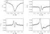 |
Fig. 4 From left to right and top to bottom: Stokes I, Q, U and V profiles (dots) of the Si i line normalized to the continuum, and best fits (solid line) using a two-component SIR inversion. The profiles correspond to [x,y] = [20 |
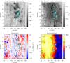 |
Fig. 5 a) The continuum intensity image show pores and orphan penumbrae at the PIL. b) The absorption in helium (red core) clearly shows the spine in the lower part of the image and a diffuse filament in the upper part. c) LOS velocity map inferred from the standard single-component inversions of SIR. The marked areas (1 − 5) correspond to the two-component Stokes V profiles (the average inclinations and velocities for these areas are presented in Table 4). d) LOS inclinations from the single-component inversions. In all maps, the cyan colored crosses mark the positions where two-component profiles were detected. |
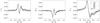 |
Fig. 6 Dots represent the observed Si i Stokes U, Q, and V profiles (same as Fig. 4). The overplotted synthetic profiles were computed using different magnetic field inclination angles for the second component, that varied between γ ∈ [40°, 120°]. The test was performed by varying the magnetic field inclination of the second component and keeping the remaining atmospheric parameters (which came from the best fit of the SIR inversion) fixed. The dotted red line shows the best matching profile, whose corresponding atmospheric parameters are shown in the caption of Fig. 4. |
4.2. Two-component Stokes V profiles at the PIL: supersonic downflows
On July 5, the day when we first observed the orphan penumbral system, we detected the presence of atypical multilobed Stokes V profiles (e.g., Fig. 4) in the Si i 10 827 Å line. These multilobed profiles are a clear indication of the presence of several magnetized components within the resolution element. Most of these multi-component profiles were found near the borders of the orphan penumbrae. To illustrate this, we selected one map from July 5 (taken between 13:39 − 13:58 UT) and marked the location of all two-component profiles with small cyan crosses (see Fig. 5). The other maps from July 5 show a similar spatial distribution of the multi-component profiles. Only points with a Stokes V/Ic signal of at least 0.01 were selected for this study. In this way, we made sure that the origin of these profiles was related to a multiple-velocity component scenario, and we were able to rule out other causes such as mixed polarities, which are also a very common occurrence in the proximity of PILs. Figure 5a shows a continuum intensity image. The two-component profiles are located on top of pores and orphan penumbrae, between x ∈ [16″,22″] . The helium red component intensity map in Fig. 5b shows that the largest group of atypical Stokes V profiles is co-spatial with the dark He i thread located around [x,y] = [20″,20″] . Only three asymmetric profiles were detected at the spine, around ![Mathematical equation: \hbox{$[x,y] = [18\farcs5,3\arcsec]$}](/articles/aa/full_html/2012/06/aa18887-12/aa18887-12-eq115.png) . The contours in Figs. 5b, c correspond to the darkest areas, i.e., highest absorption of the He i red component, of Fig. 5b. Bear in mind that the multi-component profiles were only found in the photosphere; there is no signature of these highly Doppler shifted components in the chromospheric He i 10 830 Å profiles. The atypical Si i profiles contain information about a strongly redshifted component that the standard SIR inversions cannot pick out. The conspicuous signature present in Stokes V calls for a two-atmosphere inversion that can provide some insights into the nature of this shifted component. Such inversions were performed on those specific profiles where this signature was visually detected. The following properties were inferred:
. The contours in Figs. 5b, c correspond to the darkest areas, i.e., highest absorption of the He i red component, of Fig. 5b. Bear in mind that the multi-component profiles were only found in the photosphere; there is no signature of these highly Doppler shifted components in the chromospheric He i 10 830 Å profiles. The atypical Si i profiles contain information about a strongly redshifted component that the standard SIR inversions cannot pick out. The conspicuous signature present in Stokes V calls for a two-atmosphere inversion that can provide some insights into the nature of this shifted component. Such inversions were performed on those specific profiles where this signature was visually detected. The following properties were inferred:
-
1.
The atypical Stokes V profiles appear at, or very close to, the PIL, i.e., where the magnetic field lines are mainly horizontal (see inclinations inferred from the standard single-component silicon inversions, γSi in Fig. 5d).
-
2.
From the two-component SIR inversions we inferred: (1) a dominant transverse component with a filling factor in the range of f1 ∈ [0.87,0.98] and inclinations with respect to the LOS γ1 ∈ [68°,95°] . This is the component that is most similar to that retrieved by the standard inversions. (2) A second component with smaller filling factors, f2 ∈ [0.02,0.13] , oriented more parallel to the LOS, with inclinations γ2 ∈ [21°,58°] .
-
3.
The inferred Doppler maps show that the dominant transverse component has velocities in the range of v1 ∈ [−0.1,0.5] km s-1 while the longitudinal one, with smaller filling factors, has downward velocities v2 ∈ [6.2,11.9] km s-1. It is clearly a supersonic downflowing component.
-
4.
In Fig. 5, all the detected atypical Stokes V profiles had a second component with the same polarity than the first one, except for the group of points between y = [11″,13″] (area 1 in Fig. 5c) which had a second component with opposite polarity to that of the first one. Note, however, that the dominant polarity, being highly transverse, is very much prone to polarity changes due to projection effects.
Mean LOS inclinations ( ⟨ γ ⟩ ) and velocities ( ⟨ v ⟩ ) inferred from the two-component inversions of the Si i line.
The multiple component profiles were grouped in five separate areas. Since the properties of the dominant and of the redshifted components differ in each of these areas, a separate statistical study for them has been carried out. The five areas are marked in Fig. 5c. Table 4 summarizes the mean LOS inclinations ( ⟨ γ ⟩ ) and velocities ( ⟨ v ⟩ ), for both components, in the five areas. The standard deviation (σ) of both quantities, as well as the number of pixels used for the statistics (#), are also listed. As stated before, the second component is completely dominated by magnetic field line inclinations which are more longitudinally orientated. These inclinations, however, vary substantially within each area (note the large values of the standard deviation σγ for Comp. 2 in Table 4). In these atypical cases, the inversion code provides considerable uncertainties associated with the atmospheric parameters, something that should be expected since this redshifted component has a small effect on the observed profiles, as reflected by its low filling factor (mostly < 0.1). However, a clear tendency for smaller inclinations, i.e., more vertically oriented field lines, is seen in all five areas.
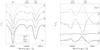 |
Fig. 7 Left: averaged intensity profiles I/Ic of four selected positions of the map acquired on July 5 between 13:39 − 13:58 UT. Each profile is marked with a character a) − d) which indicates its position in Fig. 2. Note the shifted red wing of the blended He i red component for the two facular profiles indicating the presence of more than one component contributing to the line formation. Right: the corresponding helium Stokes V/Ic profiles to the intensity profiles shown on the left panel. The solid lines along the x-axis indicate V/Ic = 0 for each profile. The dotted vertical lines, in both panels, mark the position of the line cores of the involved ions. |
Given the small amplitude of the signatures that this component leaves on the emergent Stokes profiles, the question is raised of how reliable the inversions are. To address this question, we performed the following test: we selected several pixels with multilobed Stokes V signals and used the atmospheres resulting from the two-component inversions to synthesize sets of Stokes profiles. For each model atmosphere, several different realizations of the synthesis, with different values of the inclinations and azimuths of the second component, were carried out (the first component was kept unchanged). Figure 6 shows one example of the synthetic Stokes Q, U, and V profiles (Stokes I showed no changes and was therefore not presented) with different inclinations, between 40° and 120°. Stokes Q and U present minor changes in their shape that are just above the noise level and therefore not conclusive. However, the changes in inclination substantially affected the resulting Stokes V profiles. It is apparent from Fig. 6 that the most likely inclination is far from being transverse. In fact, the best fit (dotted red line) yields an inclination of γ = 22.9° ± 20°. We also carried out the same test changing the azimuth. Stokes Q and U were only slightly affected by these variations, again within the noise level, while Stokes V was completely insensitive to the changes. This shows that while the inclination of the redshifted component is well established (and that it is more vertical than the dominant, transverse, component), the value of its azimuth is highly uncertain.
4.3. Ubiquitous downflows around the PIL in the helium velocity maps
As mentioned above, the velocities inferred from the He i inversions outside the PIL (in the faculae) are ubiquitously dominated by downflows on both days (see the lower panels of Fig. 3). This was largely unexpected, so it is important to understand what signature in the spectral profiles made MELANIE infer these downflows. Figure 7 shows four representative Stokes I and V profiles from different areas of the map taken between 13:39 − 13:58 UT on July 5. They correspond to: (a) the spine; (b) the PIL; (c) the negative and (d) the positive polarities within the faculae. The locations of pixels a − d are marked in Fig. 2. The dotted vertical lines, in Fig. 7, mark the centers of the line cores at rest. In the lefthand panel, the intensity spectra comprise the photospheric Si i line and the He i triplet. The cores of the four silicon intensity profiles are almost perfectly centered at their rest wavelengths. However, while the He i triplet profiles of the spine and the PIL are also approximately at rest, the two facular profiles are clearly redshifted. It is also of interest that the red wing of the He i red component of the facular profiles is stretched away from the line core. This, together with the fact that the profiles are not symmetric, indicates that more than one atmospheric component was involved in the line formation process, and that one of these components harbors distinct downflows. The redshift in the helium red component of the facular regions is also seen in their Stokes V profiles (c and d) in the righthand panel of Fig. 7. As expected, profile (b) has almost no Stokes V signal since it is located at the PIL, where the transverse fields dominate.
It is, thus, clear that the facular profiles seen in the chromosphere are substantially redshifted. A possible explanation for this is given in Sect. 5. To quantify the general trend of the facular velocities found in our data sets we did averages only taking into account those pixels which had photospheric inclinations close to longitudinal (γSi < 25° and γSi > 155°). Note that the inclinations we used are the ones inferred from the Si i 10 827 Å inversions, whereas the velocities correspond to the ones obtained from the He i 10 830 Å inversions. This criterion ideally distinguishes the points belonging to the faculae (having mainly longitudinal fields at photospheric heights, Martinez Pillet et al. 1997) from those of other areas, such as the PIL or outside the faculae. The mean velocities found in the faculae, for all maps (July 3 and 5), were in the range of  km s-1. The standard deviations associated to these velocities were typically around σ = 1.0 − 1.4 km s-1, and the number of points used for the statistics of each map was between 300 − 400. As mentioned above, since these He i intensity profiles are likely to comprise more than one component, multi-component inversions in this spectral region (e.g., Lagg et al. 2007; Sasso et al. 2011) might reveal slightly stronger downflows in the faculae.
4.4. Time series
A time series with the slit fixed over the PIL was acquired on July 5, approximately between x ~ 18″−20″ on the righthand panel of Fig. 2. The velocities shown in Fig. 8 were retrieved from the standard Si i inversions. Time is represented along the x-axis while the y-axis shows the spatial direction along the slit. In the lower half of the figure, the photospheric 5 min oscillation is unequivocal. This corresponds to the area below the spine. There is an apparent phase shift of the oscillation pattern, starting at y ~ 15″. This shift coincides with the beginning of the orphan penumbrae. The single most striking finding from this figure was the continuous downflow seen between y ~ 23″−25″ (dark red pattern) throughout the whole time range, with which not even the photospheric oscillation pattern interfered.
The Stokes V profiles were carefully inspected one by one along the slit every minute. This was done in order to find the atypical multilobed Stokes V profiles defined in Sect. 4.2. As in Fig. 5, the cyan crosses in Fig. 8 represent the location of the detected atypical Stokes V profiles. From this figure it is obvious that the lifetime of the supersonic downflow was at least as long as our time series (19 min). We take this time to be a lower limit but it might, in fact, be much longer, since this supersonic downflow was not an isolated event. Other strong downflows have been detected on all maps from July 5 (albeit not continuously), starting from 7:36 until 14:51 UT.
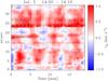 |
Fig. 8 Photospheric velocity time evolution. The time series was taken with the slit fixed on top of the PIL (between x ~ 18″−20″ in the second column of Fig. 2). The velocities were inferred from the “standard” Si i 10 827 Å inversions. The cyan-colored crosses mark the positions of the two-component profiles. |
5. Discussion
In this paper, we have investigated the LOS velocities inferred from chromospheric and photospheric spectropolarimetric inversions of the Stokes profiles measured in and below an AR filament. The aim of this study, together with the results of Paper I, is to clarify the formation and evolution of this AR filament. In Paper I we reported that the magnetic field configuration of the spine of the filament is compatible with a flux rope topology (on July 3, and also in the spine portion of July 5). Furthermore, the orphan penumbral region of July 5, was also likely to be the imprint of a flux rope, but with its axis sitting low in the photosphere. These results are supported by recent magnetic field extrapolations of the same filament by Yelles Chaouche et al. (2012) who, for July 5, also deduced the presence of a flux rope structure whose axis lay below the formation height of the He i 10 830 Å lines. Our AR filament is, therefore, extremely low-lying.
The next question that needs to be addressed is the mechanism by which flux ropes in AR filaments are formed. First of all, at the time of the observing run, the filament had already reached the chromosphere. However, on July 5, the low-lying magnetic structure and the newly appeared pores and orphan penumbrae indicated that new flux had emerged between the two days of observation. This flux was mainly horizontal due to its proximity to the PIL, as reported in Paper I. Thus, we placed special emphasis on the study of the photospheric LOS velocities associated with these transverse fields, i.e., inferred from what we called the silicon “magnetic” inversions, which provided information similar to that of the Dopplergrams of the magnetic component presented by Okamoto et al. (2009) and Lites et al. (2010). There is a very good agreement among the velocities from all maps of July 5 (see Table 3). All the maps but one pointed to an upward movement of the photospheric transverse fields, with average velocities between = −0.21 and −0.28 km s-1, the last map being the exception, where slower upward motions (~−0.10 km s-1) are shown. These velocities agree surprisingly well with the ones presented by Okamoto et al. (2009) (−0.30 ± 0.20 km s-1). However, when carrying out “standard” inversions (weighting all four Stokes parameters in the inversion equally) the average inferred velocities were close to zero or positive (downflows), with values between ⟨ vSi ⟩ = 0.02−0.11 km s-1 and 0.21 km s-1 for the last map. Note that the differences between both inversions is, on average, of around 0.3 km s-1. This is indeed a small number. It corresponds to 11 mÅ or, equivalently, a sixth of the spectral resolution. The fact that we obtain velocities that are more redshifted when we weight Stokes I and V equally in the inversion indicates that a longitudinal component harboring downflows is present, to some degree, in all pixels. While no evidence for this is provided here, we hypothesize that the same chromospheric downflow that is observed almost everywhere in He i has an impact on the Si i data, producing slightly more redshifted values when all Stokes parameters are equally weighted in the inversion code.
In the chromosphere above the orphan penumbrae, the retrieved mean LOS velocities are dominated by downflows in the range of ⟨ vHe ⟩ = 0.18−0.55 km s-1. Nevertheless, these averaged velocities need to be interpreted with caution since the helium velocity maps of Fig. 3 clearly show localized upflows and slower downward motions at the PIL (inside the green contours). These upward motions at the PIL reach velocities of about − 1 km s-1 in all the maps of July 5. A continuous upflow of mass, lasting at least ~7 h, is detected at some locations of the PIL. Since helium traces the upper part of the flux rope (whose axis is lying below, in the photosphere), these localized upflows strongly suggest that the material is being pushed upward by the magnetic field lines of the top of the flux rope (similar to what is seen in the simulations by Martínez-Sykora et al. 2008). This is in agreement with previous simulations of flux rope emergence (e.g., Fan 2001; Manchester et al. 2004; Archontis et al. 2004; Fan 2009), where only the upper field lines are able to rise and expand in the corona, leaving the main body of the flux tube behind. This process is driven by the so-called Parker instability. This interpretation would lead to plasma drainage wherever the field lines are not horizontal or dipped, and, hence, would explain the photospheric downflows close to the PIL. Sometimes, the downflows at the orphan penumbrae produce atypical multilobed Stokes V profiles. Examples of these were found in some areas near the PIL (see Fig. 5). Two-component inversions of these Stokes V profiles yielded mainly supersonic speeds, in the range of 6 − 12 km s-1, for the redshifted component. Similar strong downflows have been detected in the past (e.g., Martinez Pillet et al. 1994; Lites et al. 2002; Shimizu et al. 2008) and have also been found in numerical models of emerging flux regions (Cheung et al. 2008). The case described by Martinez Pillet et al. (1994) is particularly relevant to this paper because it describes a downflow below an AR filament, similar to the ones studied here. Magnetic reconnection is one of the proposed mechanisms to cause these supersonic downflows as suggested from the simulations of Cheung et al. (2008). In our data sets, this could only have taken place in the photosphere which is where we see them clearly. The long periods of time (tens of minutes) during which the redshifted flows persist basically unaltered, almost rule out any link with a fast process such as reconnection. The downflows might also be interpreted as a combination of plasma draining from the flux rope’s body during its emergence process at the photosphere and/or the continuation of the ubiquitous chromospheric downflows.
The filament formation model of van Ballegooijen & Martens (1989) would expect horizontal field lines submerging at the PIL after a magnetic reconnection event (van Ballegooijen & Mackay 2007). While strong downflows in our observations are clearly detected at several positions along the PIL, they are never co-spatial with transverse magnetic fields. The inclinations retrieved from the inversions of the atypical Stokes V profiles, showed that the second component (the strongly redshifted one) was much more longitudinally orientated (γ2 ∈ [21°,58°] ) than the first one (γ1 ∈ [68°,95°] ) (see more details in Table 4). Our test inversions support the reliability of these results (see Fig. 6). Therefore, we can safely say that our AR filament presents no evidence of submerging horizontal field lines, thus, challenging some features of the aforementioned models.
Let us consider now the spine of the filament, which was seen in the middle of the FOV on July 3 and only in its lower part on July 5. This portion of the filament is what we would call a classical case of AR filament, “classical” meaning that it has a thin elongated shape presenting a flux rope topology and is located in the chromosphere (it is perfectly discernible in the He i absorption image of Fig. 2). There is a distinct difference between the chromospheric LOS velocities of both days. On July 3, the spine is completely dominated by upflows which perfectly trace the transverse fields (see black contour in the lower left panel of Fig. 3). The average upward velocity inside this black contour was ⟨ vHe ⟩ ~ −0.24 km s-1. On July 5, however, the spine is not as strongly blueshifted, characteristic that continues throughout the day (see Fig. 3). Downflows in the range of ⟨ vHe ⟩ ~ 0.81 and 1.09 km s-1, are detected in the ~7 h between the first and last maps. We interpret this result as a halt in the rise of the filament’s axis. This event makes the spine area be dominated by the same ubiquitous chromospheric downflows that are seen in the rest of the FOV.
The photospheric motions of the spine on July 3 show the same trend as the chromospheric ones, with average upflows of the transverse fields of ~ −0.15 km s-1. We interpret this as a coordinated upflow of the entire flux rope. This is compatible with the flux rope emergence simulations, in which the whole structure is very low-lying. On July 5, the transverse fields begin the day moving upward = − 0.19 km s-1, but after ~2 h they seem to stop, still remaining at rest by the end of the observing run, four hours later.
We found ubiquitous downflows in the chromosphere, on both sides of the PIL. This was consistent throughout all of our observations. The average LOS velocity in the faculae, for all maps, was 1.6 km s-1 with a dispersion of ~1.2 km s-1. We hypothesize that these downflows are a manifestation of the so-called coronal rain. This phenomenon occurs when plasma condenses in the corona and then flows along coronal loops, down into ARs (Tandberg-Hanssen 1995). So far, however, our knowledge of this process is still rather poor (but see Antolin & Rouppe van der Voort 2012). Recent studies reveal that the velocities found in coronal rain are in a range between 20−120 km s-1 (Antolin et al. 2010; Antolin & Verwichte 2011; Antolin & Rouppe van der Voort 2012). This is much faster than the velocities obtained from our data (Fig. 3), although our measurements correspond to lower heights. There is a strong possibility that more than one atmospheric component, along the LOS, contributes to the He i 10 830 Å triplet formation. This can be deduced from the shape of the red wings of the intensity profiles in the faculae (lefthand panel; Fig. 7). However, the signature is weak and, hence, it is unclear whether strong downflows, such as those reported by previous authors in the He i triplet (~42 km s-1, e.g., Muglach et al. 1997; Schmidt et al. 2000; Lagg et al. 2007), would be inferred in a multi-component analysis. Another explanation could be that material is falling from the slowly rising flux rope structure on July 3, or from the expanding field lines above the orphan penumbrae on July 5, following vertical magnetic field lines (in a similar way as the draining of rising loops proposed by Lagg et al. 2007). However, these processes can also be considered to be different manifestations of the coronal-rain phenomenon.
6. Conclusions
For the sake of clarity we divided the study of the AR filament into two parts, the main distinction between them being the height at which the filament axis lies. The first part corresponds to the spine (seen mainly on July 3, and also in the lower half of the FOV on July 5), where the filament axis lies in the chromosphere. The second corresponds to the diffuse filament (seen only in the upper half of the FOV on July 5), which sits above the orphan penumbrae and pore regions, and has a much lower-lying filament axis. In this latter case, the helium 10 830 Å only traces the upper part of the flux rope, as explained in Paper I. The main conclusions of this study are:
-
1.
On July 3, the LOS velocities inferred from the helium and“magnetic” silicon inversions (that trace thebehavior of the horizontal magnetic fields) in the spine re-gion, show generalized upflows, which we interpret to rep-resent the emergence of the flux rope structure as a whole.Two days later, on July 5,the spine shows downflows in the chromo-sphere, similar to those seen elsewhere in thefacular region. Yet the photospheric velocities inthis region present upflows for the first few hoursof the day that drop to velocities close to zero toward the end ofthe observing run.
-
2.
On July 5, in the chromosphere, above the orphan penumbrae, the LOS velocities are on average redshifted. This redshift is, however, smaller than the dominant redshift seen in the facular region. Indeed, blueshifted patches are present along the PIL in all data sets. We propose that the blueshifted patches seen in the chromosphere are due to field lines which expand from the lower-lying flux rope into the chromosphere, similar to what is found in the flux rope emergence simulations (e.g., Martínez-Sykora et al. 2008). The photospheric transverse field lines along the orphan penumbrae are clearly moving upward. This is consistent in all seven data sets. Therefore the sheared field lines (the flux rope axis) are rising.
-
3.
Atypical multilobed Stokes V profiles were found in the photosphere near the PIL. Two-component inversions of these profiles revealed localized supersonic downflows in the strongly redshifted component. These downflows last for at least 19 min, ruling out any episodic origin. Furthermore, the retrieved magnetic fields associated with this component are oriented along (or very close to) the line of sight. Therefore, we cannot identify this component with submerging loops that harbor horizontal fields as in the models from van Ballegooijen & Martens (1989) and van Ballegooijen & Mackay (2007). It is also important to point out that the number of detected two-component profiles was only a small percentage of the total number of points inside the PIL (12%), which, on average, showed an upward motion of the transverse fields.
-
4.
Almost ubiquitous redshifts of the chromospheric He i 10 830 Å triplet, with average downflows of ~1.6 km s-1 and a dispersion of ~1.2 km s-1, were found in the faculae in all data sets.
The global picture resulting from the Doppler shifts studied in this paper can be summarized as follows. AR faculae are immersed in a global rainfall of mass from the upper layers, as indicated by the redshifted He i line. We have tentatively associated this redshift with coronal rain. This process has no evident counterpart in the photosphere, being some localized supersonic downflows the only possible candidate. In this environment, the transverse field lines (including the filament axis observed either in the chromosphere or in the photosphere) display upflows. The only case where this does not hold true is that of the chromospheric spine region on July 5. In this area, only the global downflow is observed.
As we have learned from the simulations, the process of flux rope emergence through the photosphere is not an easy one and will often be aborted. We propose that this is what might have happened on July 5 at the spine region. Note, however, that the rest of the filament for this day displayed clear upflows at both heights. All in all, the present study supports the scenario of an emerging flux rope from below the photosphere. Vector magnetograms, as well as LOS velocities in the photosphere and chromosphere, agree with the proposed scenario. Whether or not this emergence process is common to all AR filaments, or at least to those that present a photospheric manifestation (orphan penumbrae), needs to be proven by using further multi-wavelength and multiheight observations.
There are some limitations in this work that need to be considered. First, an important observational gap on July 4 exists. Data from that day would have contributed to a better understanding of the inferred magnetic structure observed on July 5. Another limitation to this work is the small FOV of the polarimeter that we had at the time of the observations (nowadays the slit is twice as large). This work has proved that there is an imperative need for multi-wavelength instruments and larger FOVs in order to understand the formation process and evolution of AR filaments. It is crucial to have magnetic field information of at least two heights, e.g., in the photosphere and in the chromosphere, to carry out a simultaneous and co-spatial analysis of the evolution of the filament.
The flux rope that constitutes the studied AR filament is extremely low-lying, especially the portion observed on the second day. This result makes it hard for the filament formation models that build flux ropes in the corona by reconnection (e.g., van Ballegooijen & Martens 1989; DeVore & Antiochos 2000) to reproduce the scenario that we observe. In particular, the large scale submergence of photospheric transverse field lines is not observed in our data. While a rather complete picture of the evolution of this AR filament (favoring a flux rope emergence from below the photosphere) has come out of this series of papers, we would like to stress that the formation process of AR filaments in general could differ, maybe substantially, from this case.
Online material
Appendix A: Velocity calibration
In order to obtain LOS velocities on an absolute scale, our Doppler shifts have to be calibrated to high precision and corrected for the systematic effects introduced by the Earth’s rotation, the orbital motion of Earth around the Sun, the solar rotation, as well as for the solar gravity redshift.
The final accuracy and precision have to be high enough to be able to measure typical photospheric Doppler shifts which, in the case of the Si i line, correspond to velocities in the range of few hundred m s-1. Since our spectral range comprises two telluric H2O lines, we can use these to calculate our sampling (Å per pixel). A Gaussian function with six terms was fit to the deepest part of these lines in our data in order to determine the position of their centers. The difference, Δx, is the distance between both lines in pixel units. The same process was carried out on the Fourier Transform Spectrometer (FTS) spectrum (Kurucz et al. 1984) from the Kitt Peak National Observatory, obtaining Δλ = 1.873 Å for the distance between both lines. The spectral sampling is merely calculated by dividing Δλ/Δx. This was done for each map using the average spectrum from a small non-magnetic region (containing about 1000 pixels). The mean spatial sampling of all maps is 11.035 ± 0.010 mÅ/px. Ideally, the sampling should always be the same. It can be theoretically calculated using the specifications of the telescope and of the spectrograph. A comparison with the theoretical sampling (11.240 mÅ/px) reveals that the calibration delivered a slightly smaller value, but not too different.
We are now able to construct the wavelength array using the calculated spectral sampling and a telluric line whose central wavelength is known, as a reference. According to the solar spectrum atlas of Swensson et al. (1970), the telluric line closest to the He i triplet has a wavelength of 10 832.120 Å, although the authors also provide another value: 10 832.150 Å. However, when we calculate the line center position using the Gaussian fit to the FTS spectrum we find a wavelength of 10 832.099 Å. Note that the wavelengths of the FTS atlas are not corrected for the gravity shift. This is perfectly adequate for telluric lines, which are, indeed, not affected by it. Other wavelength values, differing slightly from those mentioned previously, can also be found in the literature. These discrepancies led us to make our own estimate for the center wavelength of the H2O telluric line. The process, explained in Appendix B, results in a wavelength of 10 832.108 Å. This value is supported by the work of Breckinridge & Hall (1973), who inferred a wavelength of 10 832.109 Å with an accuracy approaching ± 1 mÅ.
The newly constructed wavelength array is referred to a terrestrial reference frame, that does not account for any relative orbital motions. We followed the calibration procedures presented in Appendix A of Martinez Pillet et al. (1997), and references therein, adapted to the Observatorio del Teide, to obtain absolute LOS velocities. Line shifts due to Earth’s rotation, orbital motion
of Earth around the Sun and solar rotation have been corrected. In the same way, the gravitational redshift, ΔλG = (GM⊙/R⊙c2)λ (which translates into 23 mÅ for this spectral range), was also corrected in our calibration. The effect of convective blueshift has been studied for the photospheric Si i line, however, after reviewing the literature and studying the response function to various physical perturbations of this line, we concluded that the correction is rather negligible owing to the formation height of the Si i line, which happens at a considerable height (log τ ~ −2) above the surface.
Appendix B: Determination of a new telluric line wavelength
As mentioned in the previous Appendix, the literature quotes several different values for the central wavelength (λT) of the H2O telluric line next to the He i triplet. We calibrated our spectrum using this telluric line as a reference, but the resulting velocity maps were clearly shifted to the red (when using λT = 10 832.120 Å) or to the blue (when using λT = 10 832.099 Å). This is, we found systematic photospheric redshifts or blueshifts (depending on the wavelength used for the calibration) in the faculae, where velocities are expected to be around zero (see Fig. 12 in Martinez Pillet et al. 1997, where high filling factor faculae show no velocity shift). Shifts on the same order of magnitude were found when compared to new data from a recent observing campaign in 2010 with the Tenerife Infrared Polarimeter at the VTT. We attribute this inconsistency to an incorrect value of the central wavelength of the telluric line and therefore we corrected its wavelength using the following method: we took three flat fields from our 2010 campaign with TIP-II (August 21 and 22); two from the morning and one from the afternoon. All of the flat fields were taken at disk center in the quiet sun, with a random circular movement of the telescope pointing of up to 50′′. These maps were then used as input data for the standard reduction procedure including flat field, dark current and polarimetric calibration corrections (Collados 1999, 2003). The spectral sampling for each flat field was inferred using the same procedure described in Appendix A. Using λT = 10 832.120 Å as the reference telluric line, a mean redshift of the Si i line of Δλ ~ 0.0117 Å was found. As mentioned above, this line is not expected to show any convective blueshift due to its formation height. Also no redshifts are expected at disk center. Thus, this systematic redshift was subtracted from the λT = 10 832.120 Å telluric line, yielding a new wavelength of  Å. With the new reference, the average photospheric facular velocity for all maps resulted in ~−0.06 km s-1. Since the faculae observed here are very compact and have large filling factors (typically, higher than 50%), this value is expected to be zero. We thus conclude that the systematic effects of our velocity calibration are smaller than 60 m s-1 or around 2 mÅ.
Acknowledgments
This work has been partially funded by the Spanish Ministerio de Educación y Ciencia, through Project No. AYA2009-14105-C06-03 and AYA2011-29833-C06-03. Financial support by the European Commission through the SOLAIRE Network (MTRN-CT-2006-035484) is gratefully acknowledged. This paper is based on observations made with the VTT operated on the island of Tenerife by the KIS in the Spanish Observatorio del Teide of the Instituto de Astrofísica de Canarias. The National Center for Atmospheric Research (NCAR) is sponsored by the National Science Foundation (NSF). B. Ruiz Cobo helped with the support and implementation of the SIR code and is gratefully acknowledged.
References
- Antolin, P., & Rouppe van der Voort, L. 2012, ApJ, 745, 152 [NASA ADS] [CrossRef] [Google Scholar]
- Antolin, P., & Verwichte, E. 2011, ApJ, 736, 121 [NASA ADS] [CrossRef] [Google Scholar]
- Antolin, P., Shibata, K., & Vissers, G. 2010, ApJ, 716, 154 [NASA ADS] [CrossRef] [Google Scholar]
- Archontis, V., Moreno-Insertis, F., Galsgaard, K., Hood, A., & O’Shea, E. 2004, A&A, 426, 1047 [NASA ADS] [CrossRef] [EDP Sciences] [Google Scholar]
- Babcock, H. W., & Babcock, H. D. 1955, ApJ, 121, 349 [Google Scholar]
- Bard, S., & Carlsson, M. 2008, ApJ, 682, 1376 [NASA ADS] [CrossRef] [Google Scholar]
- Borrero, J. M., Bellot Rubio, L. R., Barklem, P. S., & del Toro Iniesta, J. C. 2003, A&A, 404, 749 [NASA ADS] [CrossRef] [EDP Sciences] [Google Scholar]
- Breckinridge, J. B., & Hall, D. N. B. 1973, Sol. Phys., 28, 15 [NASA ADS] [CrossRef] [Google Scholar]
- Chae, J., Park, H.-M., & Park, Y.-D. 2007, J. Kor. Astron. Soc., 40, 67 [NASA ADS] [CrossRef] [Google Scholar]
- Cheung, M. C. M., Schüssler, M., Tarbell, T. D., & Title, A. M. 2008, ApJ, 687, 1373 [NASA ADS] [CrossRef] [Google Scholar]
- Collados, M. 1999, in Third Advances in Solar Physics Euroconference: Magnetic Fields and Oscillations, ed. B. Schmieder, A. Hofmann, & J. Staude, ASP Conf. Ser., 184, 3 [Google Scholar]
- Collados, M. V. 2003, in SPIE Conf. Ser. 4843, ed. S. Fineschi, 55 [Google Scholar]
- Collados, M., Lagg, A., Díaz Garcí A, J. J., et al. 2007, in The Physics of Chromospheric Plasmas, ed. P. Heinzel, I. Dorotovič, & R. J. Rutten, ASP Conf. Ser., 368, 611 [Google Scholar]
- Demoulin, P., Malherbe, J. M., Schmieder, B., & Raadu, M. A. 1987, A&A, 183, 142 [NASA ADS] [Google Scholar]
- DeVore, C. R., & Antiochos, S. K. 2000, ApJ, 539, 954 [NASA ADS] [CrossRef] [Google Scholar]
- Fan, Y. 2001, ApJ, 554, L111 [NASA ADS] [CrossRef] [Google Scholar]
- Fan, Y. 2009, ApJ, 697, 1529 [NASA ADS] [CrossRef] [Google Scholar]
- Ioshpa, B. A., & Obridko, V. N. 1999, in Magnetic Fields and Solar Processes, ed. A. Wilson, et al., ESA SP, 448, 497 [NASA ADS] [Google Scholar]
- Kuckein, C., Centeno, R., Martínez Pillet, V., et al. 2009, A&A, 501, 1113 [NASA ADS] [CrossRef] [EDP Sciences] [Google Scholar]
- Kuckein, C., Martínez Pillet, V., & Centeno, R. 2012, A&A, 539, A131 [NASA ADS] [CrossRef] [EDP Sciences] [Google Scholar]
- Kupka, F., Piskunov, N., Ryabchikova, T. A., Stempels, H. C., & Weiss, W. W. 1999, A&AS, 138, 119 [NASA ADS] [CrossRef] [EDP Sciences] [MathSciNet] [PubMed] [Google Scholar]
- Kurucz, R. L., Furenlid, I., Brault, J., & Testerman, L. 1984, Solar flux atlas from 296 to 1300 nm, ed. R. L. Kurucz, I. Furenlid, J. Brault, & L. Testerman [Google Scholar]
- Lagg, A., Woch, J., Solanki, S. K., & Krupp, N. 2007, A&A, 462, 1147 [NASA ADS] [CrossRef] [EDP Sciences] [Google Scholar]
- Lin, Y., Engvold, O., Rouppe van der Voort, L., Wiik, J. E., & Berger, T. E. 2005, Sol. Phys., 226, 239 [NASA ADS] [CrossRef] [Google Scholar]
- Lites, B. W., Low, B. C., Martinez Pillet, V., et al. 1995, ApJ, 446, 877 [NASA ADS] [CrossRef] [Google Scholar]
- Lites, B. W., Socas-Navarro, H., Skumanich, A., & Shimizu, T. 2002, ApJ, 575, 1131 [NASA ADS] [CrossRef] [Google Scholar]
- Lites, B. W., Kubo, M., Berger, T., et al. 2010, ApJ, 718, 474 [NASA ADS] [CrossRef] [Google Scholar]
- Mackay, D. H., Karpen, J. T., Ballester, J. L., Schmieder, B., & Aulanier, G. 2010, Space Sci. Rev., 151, 333 [NASA ADS] [CrossRef] [Google Scholar]
- MacTaggart, D., & Hood, A. W. 2010, ApJ, 716, L219 [NASA ADS] [CrossRef] [Google Scholar]
- Malherbe, J. M., Schmieder, B., Ribes, E., & Mein, P. 1983, A&A, 119, 197 [NASA ADS] [Google Scholar]
- Manchester, IV, W., Gombosi, T., DeZeeuw, D., & Fan, Y. 2004, ApJ, 610, 588 [NASA ADS] [CrossRef] [Google Scholar]
- Martinez Pillet, V., Lites, B. W., Skumanich, A., & Degenhardt, D. 1994, ApJ, 425, L113 [NASA ADS] [CrossRef] [Google Scholar]
- Martinez Pillet, V., Lites, B. W., & Skumanich, A. 1997, ApJ, 474, 810 [NASA ADS] [CrossRef] [Google Scholar]
- Martínez-Sykora, J., Hansteen, V., & Carlsson, M. 2008, ApJ, 679, 871 [NASA ADS] [CrossRef] [Google Scholar]
- Martres, M.-J., Rayrole, J., & Soru-Escaut, I. 1976, Sol. Phys., 46, 137 [NASA ADS] [CrossRef] [Google Scholar]
- Martres, M.-J., Mein, P., Schmieder, B., & Soru-Escaut, I. 1981, Sol. Phys., 69, 301 [NASA ADS] [CrossRef] [Google Scholar]
- Mein, P. 1977, Sol. Phys., 54, 45 [NASA ADS] [CrossRef] [Google Scholar]
- Muglach, K., Schmidt, W., & Knoelker, M. 1997, Sol. Phys., 172, 103 [NASA ADS] [CrossRef] [Google Scholar]
- Murray, M. J., Hood, A. W., Moreno-Insertis, F., Galsgaard, K., & Archontis, V. 2006, A&A, 460, 909 [NASA ADS] [CrossRef] [EDP Sciences] [Google Scholar]
- Okamoto, T. J., Tsuneta, S., Lites, B. W., et al. 2008, ApJ, 673, L215 [NASA ADS] [CrossRef] [Google Scholar]
- Okamoto, T. J., Tsuneta, S., Lites, B. W., et al. 2009, ApJ, 697, 913 [NASA ADS] [CrossRef] [Google Scholar]
- Ruiz Cobo, B., & del Toro Iniesta, J. C. 1992, ApJ, 398, 375 [NASA ADS] [CrossRef] [Google Scholar]
- Sasso, C., Lagg, A., & Solanki, S. K. 2006, A&A, 456, 367 [NASA ADS] [CrossRef] [EDP Sciences] [Google Scholar]
- Sasso, C., Lagg, A., & Solanki, S. K. 2011, A&A, 526, A42 [NASA ADS] [CrossRef] [EDP Sciences] [Google Scholar]
- Schmidt, W., Muglach, K., & Knölker, M. 2000, ApJ, 544, 567 [NASA ADS] [CrossRef] [Google Scholar]
- Schmieder, B., Malherbe, J. M., Simon, G., & Poland, A. I. 1985, A&A, 153, 64 [NASA ADS] [Google Scholar]
- Schmieder, B., Chandra, R., Berlicki, A., & Mein, P. 2010, A&A, 514, A68 [NASA ADS] [CrossRef] [EDP Sciences] [Google Scholar]
- Shimizu, T., Lites, B. W., Katsukawa, Y., et al. 2008, ApJ, 680, 1467 [NASA ADS] [CrossRef] [Google Scholar]
- Socas-Navarro, H. 2001, in Advanced Solar Polarimetry – Theory, Observation, and Instrumentation, ed. M. Sigwarth, ASP Conf. Ser., 236, 487 [Google Scholar]
- Socas-Navarro, H., Trujillo Bueno, J., & Landi Degl’Innocenti, E. 2004, ApJ, 612, 1175 [NASA ADS] [CrossRef] [Google Scholar]
- Swensson, J. W., Benedict, W. S., Delbouille, L., & Roland, G. 1970, Mem. Soc. Roy. Sci. Liege, 5 [Google Scholar]
- Tandberg-Hanssen, E. 1995, The nature of solar prominences, Astrophys. Space Sci. Libr., 199 [Google Scholar]
- van Ballegooijen, A. A., & Mackay, D. H. 2007, ApJ, 659, 1713 [NASA ADS] [CrossRef] [Google Scholar]
- van Ballegooijen, A. A., & Martens, P. C. H. 1989, ApJ, 343, 971 [NASA ADS] [CrossRef] [Google Scholar]
- von der Lühe, O., Soltau, D., Berkefeld, T., & Schelenz, T. 2003, in SPIE Conf. Ser. 4853, ed. S. L. Keil, & S. V. Avakyan, 187 [Google Scholar]
- Welsch, B. T., & Fisher, G. H. 2012 [arXiv:1201.2451] [Google Scholar]
- Yelles Chaouche, L., Cheung, M. C. M., Solanki, S. K., Schüssler, M., & Lagg, A. 2009, A&A, 507, L53 [NASA ADS] [CrossRef] [EDP Sciences] [Google Scholar]
- Yelles Chaouche, L., Kuckein, C., Martínez Pillet, V., & Moreno-Insertis, F. 2012, ApJ, 748, 23 [NASA ADS] [CrossRef] [Google Scholar]
All Tables
Examples of the LOS to local solar reference frame transformation of the magnetic field inclination and azimuth.
Mean Doppler velocities ( ⟨ v ⟩ ), of all available maps for both days, calculated inside the contours, where the inferred LOS inclinations are between 75° < γ < 105°, i.e., along the PIL.
Mean LOS inclinations ( ⟨ γ ⟩ ) and velocities ( ⟨ v ⟩ ) inferred from the two-component inversions of the Si i line.
All Figures
|
Fig. 1 Stokes I profile, normalized to the continuum intensity, observed by TIP-II near the PIL. The dashed vertical lines indicate the positions of the rest wavelengths for the spectral lines that are used in this work. |
| In the text | |
|
Fig. 2 TIP-II slit-reconstructed images for both days of observation. From top to bottom: continuum, Si i line core intensity, He i line core intensity (red component) and Si i Stokes V. The FOV was different on July 3 and July 5. We provide the dashed rectangles to show the approximate common area of the filament on both days. Characters a) − d) indicate the position of the Stokes profiles presented in Fig. 7. The white arrows point to high concentrations of helium with elongated shapes (thread-like structures). |
| In the text | |
|
Fig. 3 LOS velocities inferred from: the Si i 10 827 Å full Stokes “standard” inversions (top row), the Si i 10 827 Å “magnetic” inversions (with weights: wI = 0, wQ,U = 1.0 and wV = 0.1) (middle row) and He i 10 830 Å inversions (bottom row) at different times. Note that the color scale is saturated at [−1, 1] and [−2, 2] km s-1 for silicon and helium respectively. Pixels inside the contours have magnetic field inclinations, with respect to the LOS, between 75° ≤ γ ≤ 105°. In the July 5 maps, the colored contours distinguish between the orphan penumbrae area (green) and the spine region (black). On July 3, only the spine of the filament was seen. Negative velocities (blue) indicate upflows while positive velocities (red) indicate downflows. |
| In the text | |
|
Fig. 4 From left to right and top to bottom: Stokes I, Q, U and V profiles (dots) of the Si i line normalized to the continuum, and best fits (solid line) using a two-component SIR inversion. The profiles correspond to [x,y] = [20 |
| In the text | |
|
Fig. 5 a) The continuum intensity image show pores and orphan penumbrae at the PIL. b) The absorption in helium (red core) clearly shows the spine in the lower part of the image and a diffuse filament in the upper part. c) LOS velocity map inferred from the standard single-component inversions of SIR. The marked areas (1 − 5) correspond to the two-component Stokes V profiles (the average inclinations and velocities for these areas are presented in Table 4). d) LOS inclinations from the single-component inversions. In all maps, the cyan colored crosses mark the positions where two-component profiles were detected. |
| In the text | |
|
Fig. 6 Dots represent the observed Si i Stokes U, Q, and V profiles (same as Fig. 4). The overplotted synthetic profiles were computed using different magnetic field inclination angles for the second component, that varied between γ ∈ [40°, 120°]. The test was performed by varying the magnetic field inclination of the second component and keeping the remaining atmospheric parameters (which came from the best fit of the SIR inversion) fixed. The dotted red line shows the best matching profile, whose corresponding atmospheric parameters are shown in the caption of Fig. 4. |
| In the text | |
|
Fig. 7 Left: averaged intensity profiles I/Ic of four selected positions of the map acquired on July 5 between 13:39 − 13:58 UT. Each profile is marked with a character a) − d) which indicates its position in Fig. 2. Note the shifted red wing of the blended He i red component for the two facular profiles indicating the presence of more than one component contributing to the line formation. Right: the corresponding helium Stokes V/Ic profiles to the intensity profiles shown on the left panel. The solid lines along the x-axis indicate V/Ic = 0 for each profile. The dotted vertical lines, in both panels, mark the position of the line cores of the involved ions. |
| In the text | |
|
Fig. 8 Photospheric velocity time evolution. The time series was taken with the slit fixed on top of the PIL (between x ~ 18″−20″ in the second column of Fig. 2). The velocities were inferred from the “standard” Si i 10 827 Å inversions. The cyan-colored crosses mark the positions of the two-component profiles. |
| In the text | |
Current usage metrics show cumulative count of Article Views (full-text article views including HTML views, PDF and ePub downloads, according to the available data) and Abstracts Views on Vision4Press platform.
Data correspond to usage on the plateform after 2015. The current usage metrics is available 48-96 hours after online publication and is updated daily on week days.
Initial download of the metrics may take a while.