| Issue |
A&A
Volume 532, August 2011
|
|
|---|---|---|
| Article Number | A134 | |
| Number of page(s) | 15 | |
| Section | Stellar atmospheres | |
| DOI | https://doi.org/10.1051/0004-6361/201116527 | |
| Published online | 05 August 2011 | |
Mid-infrared interferometric monitoring of evolved stars
The dust shell around the Mira variable RR Aquilae at 13 epochs⋆,⋆⋆
1
European Southern Observatory, Karl-Schwarzschild-Str. 2, 85748 Garching bei München, Germany
e-mail: This email address is being protected from spambots. You need JavaScript enabled to view it.
; This email address is being protected from spambots. You need JavaScript enabled to view it.
2
United States Naval Observatory, 3450 Massachusetts Avenue, NW, Washington, DC 20392-5420, USA
3
Laboratoire Univ. d’Astroph. de Nice (LUAN), CNRS UMR 6525, Parc Valrose, 06108 Nice Cedex 02, France
4
Max-Planck-Institut für Radioastronomie, Auf dem Hügel 69, 53121 Bonn, Germany
5
Zentrum für Astronomie der Universität Heidelberg (ZAH), Institut für Theoretische Astrophysik, Albert-Ueberle-Str. 2, 69120 Heidelberg, Germany
6
Sydney Institute for Astronomy, School of Physics, University of Sydney, Sydney NSW 2006, Australia
Received: 14 January 2011
Accepted: 20 June 2011
Abstract
Aims. We present a unique multi-epoch infrared interferometric study of the oxygen-rich Mira variable RR Aql in comparison to radiative transfer models of the dust shell. We investigate flux and visibility spectra at 8–13 μm with the aim of better understanding the pulsation mechanism and its connection to the dust condensation sequence and mass-loss process.
Methods. We obtained 13 epochs of mid-infrared interferometry with the MIDI instrument at the VLTI between April 2004 and July 2007, covering minimum to pre-maximum pulsation phases (0.45–0.85) within four cycles. The data are modeled with a radiative transfer model of the dust shell where the central stellar intensity profile is described by a series of dust-free dynamic model atmospheres based on self-excited pulsation models. We examined two dust species, silicate and Al2O3 grains. We performed model simulations using variations in model phase and dust shell parameters to investigate the expected variability of our mid-infrared photometric and interferometric data.
Results. The observed visibility spectra do not show any indication of variations as a function of pulsation phase and cycle. The observed photometry spectra may indicate intracycle and cycle-to-cycle variations at the level of 1–2 standard deviations. The photometric and visibility spectra of RR Aql can be described well by the radiative transfer model of the dust shell that uses a dynamic model atmosphere describing the central source. The best-fitting model for our average pulsation phase of  includes the dynamic model atmosphere M21n (Tmodel = 2550 K) with a photospheric angular diameter of θPhot = 7.6 ± 0.6 mas, and a silicate dust shell with an optical depth of τV = 2.8 ± 0.8, an inner radius of Rin = 4.1 ± 0.7 RPhot, and a power-law index of the density distribution of p = 2.6 ± 0.3. The addition of an Al2O3 dust shell did not improve the model fit. However, our model simulations indicate that the presence of an inner Al2O3 dust shell with lower optical depth than for the silicate dust shell can not be excluded. The photospheric angular diameter corresponds to a radius of
  and an effective temperature of Teff ~ 2420 ± 200 K. Our modeling simulations confirm that significant intracycle and cycle-to-cycle visibility variations are not expected for RR Aql at mid-infrared wavelengths within our uncertainties.
Conclusions. We conclude that our RR Aql data can be described by a pulsating atmosphere surrounded by a silicate dust shell. The effects of the pulsation on the mid-infrared flux and visibility values are expected to be less than about 25% and 20%, respectively, and are too low to be detected within our measurement uncertainties.
Key words: techniques: interferometric / stars: AGB and post-AGB / stars: atmospheres / stars: mass-loss / stars: individual: RR Aql
Based on observations made with Very Large Telescope Interferometer (VLTI) at the Paranal Observatory under program IDs 073.D-0711, 075.D-0097, 077.D-0630, and 079.D-0172.
Figure 5 is available in electronic form at http://www.aanda.org
© ESO, 2011
1. Introduction
Asymptotic giant branch (AGB) stars are low-to-intermediate mass stars at the end of their stellar evolution. These stars, including Mira type stars, exhibit many complex processes such as shock fronts propagating through the stellar atmosphere, large-amplitude pulsation, and molecule and dust formation leading to strong mass loss via a dense and dusty outflow from an extended stellar atmosphere (Andersen et al. 2003). The mass loss rates can reach up to 10-4 M⊙ yr-1 (Matsuura et al. 2009) with expansion velocities of 5–30 km s-1 (Höfner & Andersen 2007). Dust grains are created by condensation from the gas phase in the very cool and dense outer part of the pulsating atmosphere. Dust created by carbon-rich stars owing to its high opacity absorbs radiation from the star, and the wind is believed to be driven by radiation pressure on the dust particles that drag gas along via collisions (Höfner 2008).
Despite remarkable progress in theoretical and observational studies, it still remains unclear whether the dust in oxygen-rich envelopes is opaque enough to drive the observed massive outflows (Woitke 2006; Höfner 2008). Because of the wind, all the matter around the core of the star is eventually returned to the interstellar medium (ISM), and the star evolves toward the planetary nebula phase, leaving the core as a white dwarf. Generally many aspects of the physics of AGB stars remain poorly understood, such as the detailed atmospheric stratification and composition of the stars, or the role of stellar pulsation and its connection to the dust formation and massive outflow. Improving our understanding of the physical processes leading to the substantial mass loss is important, as AGB stars play a crucial role in the chemical enrichment and evolution of galaxies by returning gas and dust to the ISM.
Thanks to their large diameters and high luminosities, Mira variables are ideal targets for high angular resolution observations. Near-infrared interferometric techniques provide detailed information regarding the conditions near the continuum-forming photosphere such as effective temperature, center-to-limb intensity variations, the stellar photospheric diameter, and its dependence on wavelength and pulsation phase (e.g., Haniff et al. 1995; Perrin et al. 1999; van Belle et al. 1996; Young et al. 2000a; Thompson et al. 2002a,b; Quirrenbach et al. 1992; Fedele et al. 2005; Ohnaka 2004; Millan-Gabet et al. 2005; Woodruff et al. 2008). New theoretical self-excited dynamic model atmospheres of oxygen-rich stars have been created and successfully applied (Tej et al. 2003; Hofmann et al. 1998; Ireland et al. 2004b,a, 2008; Wittkowski et al. 2008).
Observations at mid-infrared wavelengths are well-suited to studying the molecular shells and the dust formation zone of evolved stars. Mid-infrared interferometry is sensitive to the chemical composition and geometry of dust shells, their temperature, inner radii, radial distribution, and the mass loss rate (e.g., Danchi et al. 1994; Monnier et al. 1997, 2000; Weiner et al. 2006). Lopez et al. (1997) presented long-term observations at 11 μm of o Ceti obtained with the Infrared Spatial Interferometer (ISI). The observed visibilities change from one epoch to the next and are not consistent with simple heating or cooling of the dust with change in luminosity as a function of stellar phase, but rather with large temporal variations in the density of the dust shell. The data were compared to axially symmetric radiative transfer models and suggest inhomogeneities or clumps. Tevousjan et al. (2004) has studied the spatial distribution of dust around four late-type stars with ISI at 11.15 μm, and find that the visibility curves change with the pulsation phase of the star. The dust grains were modeled as a mixture of silicates and graphite. The results suggest that the dust shells appear to be closer to the star at minimum pulsation phase, and farther away at maximum phase, which is also demonstrated by Wittkowski et al. (2007). Ohnaka et al. (2007) reported on temporal visibility variations of the carbon-rich Mira variable V Oph with the instruments VINCI and MIDI at the VLTI. This temporal variation of the N-band angular sizes is largely governed by the variations in the opacity and the geometrical extension of the molecular layers (C2H2 and HCN) and the dust shell (amC + SiC).
Additional information to the near- and mid-infrared observations can be obtained with Very Long Baseline Array (VLBA) observations, which allow one to study the properties of the circumstellar environment of evolved stars using the maser radiation emitted by some molecules, most commonly SiO, H2O, and OH. By observing the maser radiation at tens to several hundred AU from the star, it is possible to determine accurate proper motions and parallaxes (Vlemmings et al. 2003), total intensity and linear polarizations (Cotton et al. 2008), and the structure of the environment of the stars (Diamond et al. 1994).
This work is part of the ongoing project of concurrent multiwavelength observations using optical long baseline interferometry (AMBER and MIDI at the VLTI) combined with radio interferometry (VLBA). We aim to investigate layers at different depths of the atmosphere and circumstellar envelope (CSE) of the stars. Previous results from this project of joint VLTI/VLBA observations for the Mira star S Ori can be found in Boboltz & Wittkowski (2005) and Wittkowski et al. (2007). Here we present results of a long-term VLTI/MIDI monitoring of the oxygen-rich Mira variable RR Aql. In addition to the VLTI/MIDI observation presented in this paper, we obtained coordinated multi-epoch VLBA observations of SiO and H2O masers towards RR Aql, which will be presented in a subsequent paper.
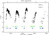 |
Fig. 1 Visual light curve of RR Aql based on data from the AAVSO and AFOEV databases as a function of Julian Date and stellar cycle/phase. The green arrows indicate the dates of our VLTI/MIDI observations. The blue arrows indicate the dates of our VLBA observations. Here, the full arrows denote observations of SiO maser emission and simple arrows observations of H2O maser emission. |
VLTI/MIDI observation of RR Aql.
2. Characteristics of RR Aql
RR Aql is an oxygen-rich Mira variable with spectral type M6e-M9 (Samus et al. 2004). RR Aql shows a strong silicate emission feature in its mid-infrared spectrum (Lorenz-Martins & Pompeia 2000). In addition, it has relatively strong SiO, H2O, and OH maser emission (Benson et al. 1990). Vlemmings & van Langevelde (2007) observed OH masers toward RR Aql at five epochs with the VLBA. Based on these observations, the distance to RR Aql is estimated to  pc (HIPPARCOS distance D = 540 pc). Van Belle et al. (2002) obtained a K-band (λ = 2.2 μm, Δλ = 0.4 μm) angular size with the Infrared Optical Telescope Array (IOTA). The uniform disk diameter (UD) of θUD = 10.73 ± 0.66 mas at phase Φ = 0.48, an effective temperature Teff = 2127 ± 111 K, and a bolometric flux fbol = 78.4 ± 11.8 × 10⁻⁸ ergs cm-2s-1. Miyata et al. (2000) studied the dust around the star spectroscopically and obtained Fdust/Fstar at 10 μm of 1.49 ± 0.02. Ragland et al. (2006) measured the closure phase with IOTA in the H-band, and classified RR Aql as a target with no detectable asymmetries. The IRAS flux at 12 μm is 332 Jy. The light curve in the V band varies from ~8 mag at maximum light to ~14 mag at minimum light. Whitelock et al. (2000) shows that the K magnitude of RR Aql varies from ~0.0 mag at maximum light to ~1.0 mag at minimum light. RR Aql is pulsating with a period of P = 394.78 days (Samus et al. 2004) and the Julian Date of the last maximum brightness is T0 = 2452875.4 (Pojmanski et al. 2005). The period of pulsation visually corresponds to recent values from the AAVSO1 and AFOEV2 databases. Figure 1 shows the visual light curve of RR Aql based on values from the AAVSO and AFOEV databases as a function of Julian day and stellar phase.
3. VLTI/MIDI observations and data reduction
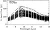 |
Fig. 2 Calibrated RR Aql MIDI flux spectra as a function of wavelength. For clarity, the error bars are omitted in the plot. |
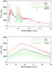 |
Fig. 3 RR Aql flux spectrum as a function of wavelength from 2.4 μm to 40 μm (top). The lines represent the flux spectra from ISO-SWS observations covering wavelengths from 2.5 μm to ~240 μm (solid red thick line), IRAS-LRS observations covering ~7.7 μm to ~23 μm (dashed thin black line), and the mean of our N-band MIDI measurements (solid thin green line). Here, the vertical bars span the maximum and minimum values measured. The diamonds denote 2MASS measurements at 1.25 μm, 1.65 μm, and 2.2 μm. The solid black line indicates our atmosphere and dust shell model as explained in Sect. 5.2. The bottom plot shows an enlarged segment of the plot in the MIDI wavelength range of 8–13 μm. |
We obtained 57 spectrally-dispersed mid-infrared interferometric observations of RR Aql with the VLTI/MIDI instrument between Apr. 9, 2004 and Jul. 28, 2007. MIDI – the mid-infrared interferometric instrument (Leinert et al. 2004) combines the beams from two telescopes of the VLTI (Glindemann et al. 2003) and provides spectrally resolved visibilities in the 10 μm window (N-band, 8–13 μm). To obtain dispersed photometric and interferometric signals, we used the PRISM as a dispersive element with a spectral resolution R = Δλ/λ ~ 30. The beams were combined in High Sens mode (HS). In this mode the photometric signal is observed after the interferometric signal.
The details of the observations and the instrumental settings are summarized in Table 1. All observations were executed in service mode using either the unit telescopes (UTs, 8.2 m) or the auxiliary telescopes (ATs, 1.8 m).
We merged the MIDI data into 15 epochs, with a maximum time-lag between individual observations of five days for each epoch (1.3% of the pulsation period). For technical problems we had to eliminate two epochs. Figure 1 shows the final 13 epochs in comparison to the light curve. The uncertainty in the allocation of the visual phase to our observations was estimated to ~0.1. Our long-term VLBA monitoring of SiO and H2O maser emission toward RR Aql, will be presented in a forthcoming paper.
We used the MIA+EWS software package, version 1.6 (Jaffe et al.3) for the MIDI data reduction. This package includes two different methods, an incoherent method (MPIA software package MIA) that analyzes the powerspectrum of the observed fringe signal and a coherent integration method (EWS), which first compensates for optical path differences, including both instrumental and atmospheric delays in each scan, and then coherently adds the fringes. We applied both methods to independently verify the data reduction results. The detector masks were calculated by the procedure of MIA, and were used for both the MIA and the EWS analysis. The obtained data reduction values correspond to each other, and we chose to use in the following the results derived from the EWS analysis, which offer error estimations.
To account for instrumental visibility losses and to determine the absolute flux values, calibrator stars with known flux and diameter values were observed immediately before or after the science target. Our main calibrators were HD 169916 (period P73, P75), HD 146051 (P77), and HD 177716 (P79). Calibrated science target visibility spectra were calculated using the instrumental transfer function derived from all calibrator data sets taken during the same night with the same baseline and instrumental mode as our scientific target. The number of available transfer function measurements depends on the number of calibrator stars observed per specific night including those calibrators observed by other programs. The errors of the transfer functions are given by the standard deviation of all transfer function measurements per night. To estimate the uncertainty of the transfer function for nights when only one calibrator was available, we used typical values based on nights when many calibrator stars were observed. The final errors on the observed visibilities are mostly systematic, and include the error of the coherence factor of the science target and the calibrators, the adopted diameter errors, and the standard deviation of the transfer function over the night.
The photometric spectrum was calibrated with one or two calibrators, which were observed close on the sky and in time compared to our science target. For most calibrator stars, absolutely calibrated spectra are available in Cohen et al. (1999). For those calibrators where the absolutely calibrated spectrum was not directly available, we instead used a spectrum of a calibrator with a similar spectral type and similar effective temperature (see the instrument consortium’s catalog4). The spectra of such calibrators were scaled with the IRAS flux at 12 μm to the level of our calibrator. In addition, we verified that our synthetic spectra obtained by this procedure are valid by scaling known spectra of two Cohen calibrators. In a few cases, when the atmospheric absorption was strongly affecting the spectra around 9.5 μm, we used another similar calibrator instead of the main calibrator observed in the same night with the same level of flux. The ambient conditions for all the observations were carefully checked. If we were facing problems with clouds, constraints due to wind, significant differences in seeing, humidity, coherence time, and airmass between the science target and the corresponding calibrator, the photometry was omitted from the analysis.
 |
Fig. 4 Calibrated RR Aql MIDI visibility amplitudes as a function of wavelength. (top left) Observations executed at projected baselines (Bp) < 20 m, (top right) 20 m < Bp < 35 m, (bottom left) 35 m < Bp < 50 m, and (bottom right) Bp > 50 m. |
4. MIDI results
We observed RR Aql at different phases over four pulsation cycles in order to monitor the mid-infrared photometry and visibility spectra. Here, we present and discuss the general properties of the data, followed by an analysis of their variability as a function of phase and cycle in Sects. 4.1 and 4.2.
Figure 2 shows all obtained calibrated photometry spectra as a function of wavelength. The MIDI flux measurements show a consistent shape exhibiting an increase in the flux from ~100–200 Jy at 8 μm to a maximum near 9.8 μm of ~200–400 Jy, and a decrease towards 13 μm, where the flux values again reach values of ~100–200 Jy. The level of the flux spectrum differs for individual measurements with a spread of ~100–200 Jy. Figure 3 shows a comparison of the mean of our MIDI flux measurements to measurements obtained with the ISO and IRAS instruments. The shape of the flux curve is consistent among the MIDI, ISO, and IRAS measurements. The level of the IRAS flux is within the range of our MIDI measurements. The level of the ISO flux is higher, which can most likely be explained by the post-maximum phase of 0.16 of the ISO observations (1997-05-03) compared to our minimum to pre-maximum phases. The difference between the MIDI and ISO flux level may also indicate a flux variation over different cycles. Figure 3 also includes a model description of our MIDI data, which is explained below in Sect. 5.2.
Figure 4 shows all obtained calibrated visibility spectra, which are combined into four groups of different projected baseline lengths (Bp) of Bp < 20 m, 20 m < Bp < 35 m, 35 m < Bp < 50 m, and Bp > 50 m. The visibility curves show a significant wavelength dependence with a steep decrease from 8 μm to ~9.5 μm and a slow increase in the 9.5 μm to 13 μm range. The shape and absolute scale of the visibility function depends on the length of the projected baseline where a longer baseline results in a lower and flatter curve.
As a first basic interpretation of the interferometric data, we computed the corresponding uniform disk (UD) diameter and the Gaussian FWHM for each data set and spectral channel. This leads to a rough estimate of the characteristic size of the target at each wavelength. However, it should be mentioned that the true intensity distribution across the stellar disk is expected to be more complex than can be described by these elementary models. Figure 5 shows for the example of epoch A, and epoch I the flux, the visibility amplitude, the corresponding UD diameter, and the corresponding Gaussian FWHM diameter as a function of wavelength. The shape of the UD diameter and Gaussian FWHM functions show a steep increase from 8 μm to ~9.5 μm by a factor of 2. A plateau appears between ~9.5 μm and 11.5 μm, and the values are nearly constant from ~1.5 μm to 13 μm.
The shape of the 8–13 μm flux spectrum with a maximum near 9.8 μm is known to be a characteristic silicate emission feature (e.g., Little-Marenin & Little 1990; Lorenz-Martins & Pompeia 2000). The corresponding drop in the visibility function between 8 μm and 9.5 μm and increase in the UD diameter and Gaussian FWHM has also been shown to be a typical signature of a circumstellar dust shell that is dominated by silicate dust (cf., e.g., Driebe et al. 2008; Ohnaka et al. 2008). The opposite trend toward a broad spectrum and visibility function in the wavelength range 8–13 μm was interpreted as a dust shell consisting of Al2O3 dust (Wittkowski et al. 2007) or silicate and Al2O3 dust (Ohnaka et al. 2005).
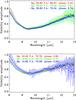 |
Fig. 6 Calibrated MIDI visibility amplitudes for different pulsation phases within the same cycle to investigate intracycle visibility variations. Each line represents a different pulsation phase within the same cycle and is computed as an average of data obtained at the respective phase ( ± 0.15) and observed at similar projected baseline length (Bp ± 10%) and position angle (PA ± 10%). The top panel shows the example of pulsation phases 0.45, 0.61, and 0.74 of cycle two observed with a projected baseline length of ~29 m and a position angle of ~70 deg. The bottom panel shows the example of pulsation phases 0.62, 0.75, and 0.83 of cycle two observed with a projected baseline length of ~16 m and a position angle of ~72 deg. The error bars are computed as the standard deviation of the averaged visibilities. |
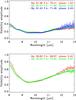 |
Fig. 7 As for Fig. 6, but for the same pulsation phase in consecutive pulsation cycles to investigate cycle-to-cycle visibility variations. The top panel shows the example of pulsation phase ~0.5 in three consecutive cycles observed with a projected baseline length of ~61 m and a position angle ~75 deg. The bottom panel shows the example of pulsation phase 0.5 in two consecutive cycles observed with a projected baseline length of ~29 m and a position angle ~70 deg. |
4.1. Visibility monitoring
We obtained a rich sample of MIDI data on RR Aql, which covers a total of four pulsation cycles and pulsation phases between 0.45 and 0.85, i.e., minimum to pre-maximum phases (see Table 1 and Fig. 1). For many different pulsation cycles and phases, we obtained data at similar projected baseline lengths and position angles. This gives us a unique opportunity to meaningfully compare interferometric data obtained at different pulsation phases and cycles. Since the visibility depends on the probed point on the uv plane, and thus on the projected baseline length and position angle, visibility data at different pulsation phases can be directly compared only if they were obtained at the same, or very similar, point on the uv plane. For this reason, we combined individual observations into groups of similar pulsation phases (Φvis ± 0.15), projected baseline lengths (Bp ± 10%), and position angles (PA ± 10%). The data within each group were averaged. The uncertainty of the averaged visibility curves was estimated as the standard deviation of the averaged visibilities.
4.1.1. Intracycle visibility monitoring
To investigate intracycle visibility variations we compared data observed at different pulsation phases within the same cycle. Figure 6 shows two examples of calibrated visibility curves, where each line in the plot represents an average of a group of visibility data, as described above, (i.e. with similar Bp, PA. and Φvis). The top panel shows an example of observations within the second pulsation cycle at phases 2.45, 2.61, and 2.74 obtained with Bp ~ 30 m and PA ~ 70°. The bottom panel shows an example of observations at phases 2.62, 2.75, and 2.83 obtained with Bp ~ 16 m and PA ~ 72°. The data do not show any evidence of intracycle visibility variations within the probed range of pulsation phases (~0.45–0.85) and within our visibility accuracies of about 5–20%.
4.1.2. Cycle-to-cycle visibility monitoring
We compared data observed at similar pulsation phases of different consecutive cycles to investigate cycle-to-cycle visibility variations. Figure 7 shows two of these examples computed in the same way as shown in Fig. 6 of Sect. 4.1.1, but (top panel) for minimum phases of 1.53, 2.59, and 3.43 in three consecutive cycles obtained with a projected baseline length of ~ 62 m and PA ~ 73°, and (bottom panel) for minimum phases 2.43, and 3.55 of two consecutive cycles obtained with a projected baseline length of ~ 29 m, and PA ~ 70°. Here, the phases of the different cycles differ by up to ~ 20%. However, we showed in Sect. 4.1.1 that there is no evidence of intracycle visibility variations, so that the chosen phases can be compared well for different cycles. As a result, Fig. 7 shows that our data do not exhibit any significant cycle-to-cycle visibility variation for minimum phases over two or three cycles within our visibility accuracies of ~5–20%.
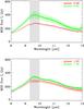 |
Fig. 8 Calibrated MIDI flux spectrum for different pulsation phases within the same cycle to investigate intracycle photometry variations. Each line represents a different pulsation phase within the same cycle and is computed as an average of data obtained at the respective phase ( ± 0.15). The top panel shows the example of pulsation phases 0.58 and 0.85 of cycle zero. The bottom panel shows the examples of phases 0.53 and 0.76 of cycle one. The error bars are computed as the standard deviation of the averaged photometry curves. The gray shades denote zones that are affected by atmospheric absorption. |
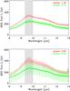 |
Fig. 9 As for Fig. 8, but for the same pulsation phase in consecutive pulsation cycles to investigate cycle-to-cycle photometry variations. The top panel shows the example of phase ~0.75 in cycles one and two. The bottom panel shows the example of phase ~0.85 of cycles zero and two. |
4.1.3. Deviations from circular symmetry
Most position angles varied around 40° or 70°. Only in two cases is the PA significantly different with values of 3° and 7°. However, in both cases the visibility data quality is poor. The differential phases are close to zero within ~10–20 deg, which is close to the calibration uncertainties that can be reached for MIDI differential phases (e.g., Ohnaka et al. 2008). Therefore these observations do not allow us to make any reliable conclusion about the presence or absence of an asymmetric intensity distribution.
Summarizing, our RR Aql MIDI data do not show any evidence of significant intracycle or cycle-to-cycle visibility variations within the examined phase coverage of ~0.45–0.85 in four consecutive cycles (see Table 1 for details of the phase coverage) and within our visibility accuracies of ~5–20%. The obtained mid-infrared interferometric observations imply either that the mid-infrared sizes of molecular and dusty layers of RR Aql do not significantly vary within our phase coverage or that the conducted observations are not sensitive enough to detect such variations. In addition, the good agreement of visibility data obtained at the same projected baseline lengths and position angles for several years also confirms the good data quality and credibility of the data reduction procedure.
4.2. N-band flux monitoring
To investigate the intracycle and cycle-to-cycle variability of our 8–13 μm flux spectra, we combined the data into groups of data obtained at similar pulsation phases (Φvis ± 0.15). The data within each group were averaged. The uncertainty of the averaged photometry curves was estimated as the standard deviation of the averaged values.
4.2.1. Intracycle photometry monitoring
Figure 8 shows two examples of a comparison of the MIDI calibrated flux spectrum at different pulsation phases of the same cycle. The top panel shows a comparison between phases 0.58 and 0.85 of cycle zero, and the bottom panel shows a comparison between phases 1.53 and 1.76 of cycle one. Both examples compare data taken at post-maximum and pre-minimum phases, i.e. with the largest separation in phase that is available in our dataset. The RR Aql flux values within the N-band are larger at the pre-maximum phases than at the post-minimum phases, corresponding to the light curve of the V-magnitude. The difference is most pronounced toward the silicate emission feature around 9.8 μm and smaller towards the edges of the MIDI bandpass at 8.0 μm and 13.0 μm. This can most likely be understood as a consequence of the silicate absorption coefficient being largest at short visual wavelengths, so that the silicate temperature is particularly sensitive to the large visual flux variations of the central star. The differences correspond to up to 20%–35%, or about one or two standard deviations.
4.2.2. Cycle-to-cycle photometry monitoring
Figure 9 shows a comparison of data observed at the same phase of consecutive pulsation cycles. The top panel shows a comparison between phases 1.76 and 2.74, i.e. phase 0.75 of cycles one and two. The bottom panel shows a comparison between phases 0.85 and 2.84, i.e phase 0.85 of cycles zero and two. In both examples, the N-band fluxes are lower in cycle two than for the same phase of (a) cycle one and (b) cycle zero by up to ~100 Jy, corresponding to about 30% or one to two standard deviations. As for the intracycle photometry variations discussed in the previous paragraph, the differences are most pronounced toward the silicate emission feature at 9.8 μm. This might indicate an irregularity in the variability cycle in the N-band. In the optical band the visual light curve clearly shows that the pulsation cycles are not perfectly symmetric (see Fig. 1).
Summarizing, our data exhibit a 1–2σ signature of intracycle, as well as cycle-to-cycle, flux variations at wavelengths of 8–13 μm, which are most pronounced toward the silicate emission feature at 9.8 μm. This indication is consistent with observations by Monnier et al. (1998), who report temporal variations in the mid-infrared spectra of late type stars. In particular, stars with a strong emission feature around 9.8 μm showed evident changes in the spectral profile. Considerable phase variation of the N-band spectra can also be found in Alvarez & Plez (1998) and Guha Niyogi et al. (2011).
5. Modeling of our MIDI data
Self-consistent models describing the dynamic atmosphere of the central source and the dust shell are still very rare. This is particularly true for oxygen-rich stars. Nevertheless, some advance in this domain has already been successfully achieved (Ireland & Scholz 2006; Höfner & Andersen 2007; Ireland et al. 2008; Höfner 2008). Here, we use an approach of an ad hoc radiative transfer modeling of the dust shell where the central stellar source is described by readily available and established dust-free dynamic model atmosphere series, as introduced by Wittkowski et al. (2007).
The dust shell surrounding the central star is modeled by the Monte Carlo radiative transfer code mcsim_mpi (Ohnaka et al. 2006). The radiative transfer model requires an assumption on the spectral energy distribution (SED) of the central stellar source. Since we expect the photosphere and molecular layers of RR Aql to be partly resolved with our MIDI baselines (V2 ~ 0.4 for θ = 10 mas, B = 120 m, λ = 10 μm), we also need to model the intensity distribution across the atmospheric layers. For these purposes, we use the dust-free dynamic model atmospheres, based on self-excited pulsation models (P and M series), by Ireland et al. (2004b,a,and references therein) as the currently best available option.
The P and M series were constructed to reproduce the M-type Mira prototypes o Cet and R Leo. The hypothetical nonpulsating “parent” stars have masses M/M⊙ = 1.0 (P series), and 1.2 (M series), Rosseland radius Rp/R⊙ = 241 (P) and 260 (M), and effective temperatures Teff = 2860 K (P) and 2750 K (M). The models have solar abundances, luminosity L/L⊙ = 3470, and a pulsation period of 332 days, close to the periods of o Cet (332 days) and R Leo (310 days). They are available for 20 phases in three cycles for the M series, and 25 phases in four cycles for the P series. These models have been shown to be consistent with broad-band near-infrared interferometric data of o Cet by Woodruff et al. (2004) and of R Leo by Fedele et al. (2005) respectively. They have also been shown to be consistent with spectrally resolved, near-infrared interferometric data of the longer period (~430 days) Mira variable S Ori exhibiting a significant variation in the angular size as a function of wavelength, which was interpreted as the effect of molecular layers lying above the continuum-forming layers as predicted by these model series (Wittkowski et al. 2008). Tej et al. (2003) indicate that the spectral shape of Mira variables can be reproduced reasonably well even for stars with different pulsation periods. In comparison with the stellar parameters of the P and M model series, RR Aql pulsates with a longer period of 394 days. The main sequence precursor mass of RR Aql is 1.2 ± 0.2 M/M⊙ (Wyatt & Cahn 1983), and its spectral type is M6e-M9 (Samus et al. 2004), versus M5-M9 (P series) and M6-M9.5 (M series). For the purpose of the modeling effort conducted here, we can assume that the general properties of the P and M model series are also valid for a longer period variable such as RR Aql. However, an exact match of model parameters and observed parameters as a function of phase may not be expected.
The flux and visibility values of the combined atmosphere and dust shell (“global“) model are computed for each spectral channel as 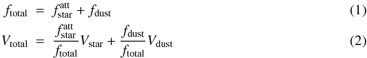 where
where  represents the attenuated flux from the dust-free model atmosphere5 (extended by a blackbody approximation for wavelengths beyond 23 μm), fdust represents the flux from the dust shell alone, ftotal is the addition of these two terms, and Vstar and Vdust are the synthetic visibilities computed for the dust-free model atmosphere and for the dust shell, respectively.
Best-fitting model parameters for each epoch.
Average model parameters.
5.1. MIDI model parameters
A clear silicate feature is identified in the spectra of RR Aql (see Fig. 3 and Sect. 4). RR Aql is one of 31 oxygen-rich stars studied by Lorenz-Martins & Pompeia (2000). The authors modeled the stars using Al2O3 and silicate grains and suggest that the dust chemistry of RR Aql contains only silicate grains. In this study we examined both of these two dust species, Al2O3 grains (Begemann et al. 1997; Koike et al. 1995) and silicates grains (Ossenkopf et al. 1992). The amount of dust is described by the optical depths at λ0 = 0.55 μm. The grain size was set to 0.1 μm for all grains. We set the photospheric radius to the well-defined continuum photospheric radius at λ = 1.04 μm (RPhot = R1.04). The density gradient was defined by a single power law ρ(r) ∝ r − p with index p. The shell thickness was set to Rout/Rin = 1000.
The global model includes seven parameters. The radiative transfer model describing the circumstellar dust shell includes six parameters: the optical depths τV (Al2O3) and τV(silicate), the inner boundary radii Rin/RPhot (Al2O3) and Rin/RPhot (silicate), and the density gradients pA (Al2O3) and pB (silicate). The model of the P/M atmosphere series is another parameter. Here, we used ten models covering one complete cycle of the M series: M16n (model visual phase Φmodel = 0.60), M18 (0.75), M18n (0.84), M19n (0.90), M20 (0.05), M21n (0.10), M22 (0.25), M23n (0.30), M24n (0.40), and M25n (0.50).
We computed a grid of dust-shell models for each of these M models, including all combinations of optical depths τV (Al2O3) = 0.0, 0.1, 0.2, 0.5, 0.8; τV (silicate) = 2.0, 2.5, 3.0, 3.5, 4.0, 4.5, 5.0; Rin/RPhot (Al2O3) = 2.0, 2.5, 3.0; Rin/RPhot (silicate) = 2.5, 3.5, 4.5, 5.5, 6.5; pA (Al2O3) = 2.0, 2.5, 3.0, 3.5; and pB (silicate) = 2.0, 2.5, 3.0, 3.5.
In a first selection of suitable models, we compared the MIDI data of each epoch to our entire grid of models. The angular diameter θPhot was the only free parameter. We increased the uncertainty of the part of the photometric spectra around 9.5 μm, which is strongly affected by telluric absorption. Otherwise, the weight of each data point was given by the corresponding uncertainty. For each epoch we kept the best ~30 models with lowest χ2 values. In a next step, a grid with finer steps around these parameters was computed. This procedure was repeated several times. The results of the automatic selection were visually inspected. We completed the selection with ten models for each epoch that agrees with the data best.
5.2. MIDI model results
For each of the 13 epochs we found the best-fitting model parameters that include the best-fitting set of dust parameters of the radiative transfer model, together with the best-fitting model of the P/M series. We used the procedure outlined in Sect. 5.1.
Following Lorenz-Martins & Pompeia (2000), we investigated dust shells including Al2O3 and/or silicate shells with different inner radii and density gradients. We obtained best-fit results with a silicate shell alone, and the addition of an Al2O3 shell did not result in any improvement in the model fits. This result is consistent with Lorenz-Martins & Pompeia (2000), who classify RR Aql as a source that can be described with a silicate dust shell alone.
The best-fitting parameters for each epoch are listed in Table 2. The table lists the epoch, the phase at the epoch, the optical depth τV, the inner boundary radius Rin/RPhot, the density distribution p, and the continuum photospheric angular diameter θPhot. Here, the dust shell parameters are those of the silicate dust shell. The errors of the dust shell parameters are derived in the same way as the standard deviation based on the find best-fitting models (Table 2). Table 3 lists the average model parameters of our different epochs. The average phase of our observations is .
The best-fitting model atmosphere was M21n (Tmodel = 2550 K, ΦModel=0.1) for all epochs covering minimum to pre-maximum pulsation phases (0.45–0.85). The difference between the average phase of our observation and the phase of the best-fitting model atmosphere can most likely be explained by the different stellar parameters of RR Aql compared to those of the M series. It means that Teff of RR Aql at the time of observation is similar to Teff of model M21n, which has a different phase, but its basic parameters are also not exactly those of RR Aql.
Figure 5 includes the model flux and model visibility compared to the observed values for the example of epoch A. For most epochs, the agreement between the models and the observed data is very good, in particular for the visibility spectra. The visibility spectra contain information about the radial structure of the atmospheric molecular layers and the surrounding dust shells. In the wavelength range from 8 μm to ~9 μm, the dust is fully resolved with baselines longer than ~20 m, and the visibility contribution of the dust reaches into the second lobe of the visibility function. RR Aql is characterized by a partially resolved stellar disk that includes atmospheric layers, with a typical drop in the visibility function ~10 μm, where the flux contribution of the silicate emission is highest and the flux contribution of the star relative to the total flux decreases. Beyond ~10 μm, the spatially resolved radiation from the optically thin dust shell starts to be a notable part of the observed total flux. From ~10 μm to 13 μm, the dust contribution becomes nearly constant while the stellar contribution increases, and this results in a rebound of the visibility function. Photometry spectra also fit well. For some epochs, the models predict higher fluxes than observed near the silicate emission feature at ~9.8 μm. Generally, our attempt at a radiative transfer model of the circumstellar dust shell that uses dynamical model atmosphere series to describe the central stellar source can reproduce the shape of both the visibility and the photometry spectra very well. Our model also follows the shape of the SED in the range of 1–40 μm (Fig. 3).
The obtained model parameters for the different epochs do not indicate any significant dependence on phase or cycle. This is consistent with the result from Sect. 4.1 that a direct comparison of visibility values of different phases or cycles did not show any variability within our uncertainties and that the photometric values indicated only small variations of up to ~2σ. However, we cannot confirm or deny an eventual phase dependence of the dust formation process that affects the 8–13 μm visibility and photometry values by less than our uncertainties of about 5–20% and 10–50%, respectively.
A silicate dust shell alone, i.e. without the addition of an Al2O3 dust shell, provides the best agreement with our data. The average optical depth of the silicate dust is τV(silicate) = 2.8 ± 0.8 at λ = 0.55 μm (corresponding to 0.03 at λ = 8 μm, 0.06 at λ = 12 μm, and a maximum within 8–12 μm of 0.22 at λ = 9.8 μm). The inner radius of the dust shell expressed in RPhot at λ = 1.04 μm is Rin = 4.1 ± 0.7 RPhot. The intensity profile of the dust-free dynamic model atmosphere extends to about 1.5–2 photosphere radii at 10 μm (cf. Wittkowski et al. 2007). The power-law index of the density distribution is p = 2.6 ± 0.3. Wind models predict a power-law index of the density distribution of 2 at radii outward the dust formation zone. However, for radii close to the dust formation zone (r < ~ 10 R ⋆ ), a larger index is expected (cf, e.g., Fig. 6 in Wittkowski et al. 2007), which is consistent with our result.
The average photospheric angular diameter results in θPhot = 7.6 ± 0.6 mas. This value is lower than the K-band (λ = 2.2 μm, Δλ = 0.4 μm) UD diameter of θUD = 10.73 ± 0.66 mas derived by van Belle et al. (2002) at a minimum phase of 0.48. This can most likely be explained by the different radius definitions. Our diameter is a photospheric angular diameter that has already been corrected for effects of molecular layers lying above the continuum photosphere using the prediction by the best-fitting model atmosphere, while the diameter by van Belle et al. is a broad-band uniform disk diameter that still contains contamination by molecular layers. It is known that broad-band UD diameters may widely overestimate the photospheric radius owing to contamination by molecular layers lying above the photosphere (cf., e.g., Ireland et al. 2004b; Fedele et al. 2005; Wittkowski et al. 2007). With the parallax of π = 1.58 ± 0.40 mas (Vlemmings & van Langevelde 2007), our value for θPhot corresponds to a photospheric radius of  . Together with the bolometric magnitude of RR Aql of mbol = 3.71 and Δmbol = 1.17 from Whitelock et al. (2000), our value for θPhot at
  corresponds to an effective temperature of Teff ~ 2420 ± 200 K. This value is consistent with the effective temperature of the best-fitting model atmosphere M21n, which is Teff = 2550 K.
Model simulations, comparing two models that differ in one or more parameters (marked by bold face).
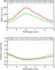 |
Fig. 10 Simulation 1. Synthetic flux (top) and visibility amplitude (bottom) in the wavelength range 8–13 μm. The solid lines represent the global models, the dashed-dotted lines denote the unattenuated stellar contribution i.e. Vstar in Eq. (2), the dotted lines denote the attenuated stellar contribution, and the dashed lines denote the dust shell contributions. This simulation compares two models consisting of the same dust shell parameters but different model atmospheres, the post-maximum model atmosphere M21n (Φmodel = 0.10), and the minimum model atmosphere M23n (Φmodel = 0.30). The photospheric angular diameter is assumed to be larger at post-maximum phase than at minimum phase (8.5 mas compared to 7 mas). The projected baseline length is 60 m. For the exact model parameters, see Table 4. They describe variations around our best-fitting model for RR Aql. |
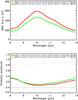 |
Fig. 11 Simulation 2. Like simulation 1 in Fig. 10, but for the parameters of simulation 2 comparing a post-maximum atmosphere model and a minimum model as in simulation 1, but where the dust is also assumed to be closer to the star with larger optical depth at minimum phase and farther from the star with lower optical depth at post-maximum phase. |
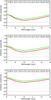 |
Fig. 13 Simulation 3. As Fig. 12, but showing the visibility spectra for different projected baseline lengths of (from top to bottom) 40 m, 25 m, and 15 m. |
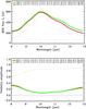 |
Fig. 14 Simulation 4. Comparison of a model with a silicate shell only and a model that also includes an Al2O3 dust shell with lower optical depth. For the model parameters, see Table 4; For the description of the figure, see the caption of Fig. 10. |
5.3. Model simulations
We performed a number of model simulations in order to investigate the visibility and photometry variations that are theoretically expected in the 8–13 μm wavelength range for the typical parameters of RR Aql as determined above in Sect. 5.2. We based our simulations on a global model with typical parameters similar to those derived for RR Aql (cf. Table 3), and investigated the effects of expected variations in the atmosphere model and the dust shell parameters during a pulsation cycle on the observable photometry and visibility spectra. We mainly used a mean projected baseline length of 60 m. As in Sect. 5, the global model consists of a radiative transfer models of the Al2O3 and silicate dust shells where the central source is described by a dust-free dynamic model atmosphere. Table 4 lists the performed simulations including the phase of the model, the optical depth τV (Al2O3) and τV (silicate), the inner boundary radii of the dust shell Rin/RPhot (Al2O3) and Rin/RPhot (silicate), the power-law indices of the density distributions p (Al2O3) and p (silicate), and the continuum photospheric angular diameter θPhot. We assume a phase dependence of the angular photospheric diameter of about 20% (Thompson et al. 2002a; Ireland et al. 2004b). Figures 10–14 show the results from the simulations. Each simulation compared two models, where one or more of the model parameters have been varied.
Simulation 1
(Fig. 10) In simulation 1, we investigate the effect of model atmospheres at different pulsation phases and effective temperatures. We compared model M21n at post-maximum pulsation phase (Φmodel = 0.10, Teff = 2550 K) and model M23n at pre-minimum pulsation phase (Φmodel = 0.30, Teff = 2230 K), applying the same dust shell parameters for both models. Here, the phase difference between M21n and M23n of 0.2 corresponds to the phase difference of our observations (~0.64 ± 0.2) The dust parameters were based on the average parameters (see Tab. 3) of RR Aql derived in Sect. 5.2. The projected baseline length was set to Bp = 60 m, which is a typical mean value of our MIDI observations. The overall shapes of the visibility spectra Vtotal (M21n) and Vtotal (M23n) are similar. The differences between the models are wavelength-dependent in the range of 5–20%. The shape of the photometry spectra are similar for both tested models ftotal (M21n) and ftotal (M23n). The largest difference of ~25% is seen around 10 μm, with less flux at minimum pulsation phase. Compared to the uncertainties of our MIDI measurements of ~5–20% in the visibility spectra and of ~20% on average in the photometric spectra, simulation 1 is consistent with our non-detection of visibility variations and a marginal detection of photometry variations.
Simulation 2
(Fig. 11) Compared to simulation 1, we adjusted the parameters according to the assumption that the outer layers of the atmosphere are cooler near minimum visual pulsation phase, and therefore more dust grains can form, and a higher molecular opacity can be expected. This theoretical assumption is consistent with mid-infrared interferometric observations (Wittkowski et al. 2007), where the observed data indicated more dust formation near minimum pulsation phase, with inner boundary radii of the dust shell located closer to the star. We increased the optical depth for model M23n. We also set a more extended dust shell after visual maximum for model M21n in comparison to the model M23n. This setting results in spectra with differences in the range of 2–19% for the visibility values. The photometry differs again mostly around 10 μm with a maximum difference of 20%. Compared to simulation 1, the results are very similar, but with less differences in the photometry spectra. As for simulation 1, the results are consistent with our not detecting visibility variations and marginally detecting photometry variations within our measurement uncertainties.
Simulation 3
(Figs. 12 and 13) Here, we investigate the effect of different dust shell parameters (as in simulation 2), but keeping the M model constant. We used model M21n (phase 0.1), which was the best-fitting model to our RR Aql epochs and also used a constant photospheric angular diameter. We compared two (silicate) dust models as in simulation 2, where in one model the optical depth is lower and the inner radius of the dust shell larger compared to the other model. These sets of model parameters lead to very similar results, where the visibility spectra almost overlap, with a maximum difference of 4% for a projected baseline length of 60 m (Fig. 12). The photometry spectra are also very similar with a maximum difference of 7%. Figure 13 shows the visibility results for different projected baseline lengths of 40 m, 25 m, and 15 m. With projected baseline lengths of less than 60 m, the difference between the visibility values become more pronounced (10% difference beyond 10 μm with projected baseline lengths of 40 m and 25 m). This can be understood because the dust shell is over-resolved with a projected baseline length of 60 m, so that the visibility cannot be sensitive to variations in the geometry of the dust shell. With lower projected baseline length, the visibility values are located in the first lobe of the visibility function, hence more sensitive to variations of the dust shell geometry. However, with the even lower projected baseline lengths of 15 m, the difference between individual models again starts to be less pronounced (<7%). This indicates an optimum projected baseline length of ~25–40 m to characterize the dust shell geometry for sizes as found for RR Aql.
Simulation 4
(Fig. 14) Furthermore, we investigate the effect of adding small amounts of Al2O3 grains to a thus far pure silicate dust shell. We examined τV(Al2O3) of 0.3 and 0.6. Figure 14 shows the simulation with τV(Al2O3) of 0.6, showing that the addition of small amounts of Al2O3 grains leads to almost identical photometry and visibility spectra (differences < 2%).
6. Discussion
Our MIDI observations of RR Aql did not show significant variations in the 8–13 μm visibility within the examined pulsation phases between 0.45 and 0.85 within a total of four pulsation cycles, and showed only marginal variations in the 8–13 μm flux.
We performed model simulations with expected variations of the pulsation phase of the innermost dust-free atmosphere model and of the parameters of the surrounding dust shells. These model simulations show that visibility variations are indeed not expected for the parameters and observational settings of RR Aql at wavelengths of 8–13 μm within the uncertainties of our observations. Variations in the flux spectra may in some cases just be detectable. Thus, our observational result of a constant visibility and only slightly varying flux at wavelengths of 8–13 μm are consistent with, and not contradicting, theoretical expectations of a pulsating atmosphere.
Our model simulations indicate that detections of pulsation effects at mid-infrared wavelengths would in particular benefit from smaller uncertainties in the photometric spectrum than in our current data. Also, a wide range of projected baselines at each phase, for RR Aql in particular including baseline lengths around 20–30 m, would help us to distinguish models of different pulsation phases.
For our analysis, we have considered silicate (Ossenkopf et al. 1992) and Al2O3 (Begemann et al. 1997; Koike et al. 1995) dust species, following the work by Lorenz-Martins & Pompeia (2000), and used fixed grain sizes of 0.1 μm. It is known that other dust species with a more complex gran size distributions may occur in the circumstellar environment of Mira variables (e.g., Höfner 2008; Molster & Waters 2003, and references therein). We showed that a model including only a silicate dust shell can reproduce the observed RR Aql visibility and flux spectrum at 8–13 μm. The addition of an Al2O3 dust shell with comparable low optical depth did not significantly improve the fit to our data. However, our model simulations have shown that our 8–13 μm visibility and flux values are not sensitive to the addition of an Al2O3 dust shell with low optical depth within our uncertainties. As a result, we cannot exclude the presence of an inner Al2O3 dust shell in addition to the silicate dust shell. Woitke (2006) uses dynamical models for dust-driven winds of oxygen-rich AGB stars, including frequency-dependent radiative transfer, and finds that dust temperatures strongly depend on material. Two dust layers are formed in his dynamical models, almost pure glassy Al2O3 close to the star (r > 1.5 Rstar) and the more opaque Fe-poor Mg-Fe-silicates farther out at 4–5 Rstar.
The dust-free dynamic model atmospheres predict a significant dependence of the characteristics of the molecular layers on the stellar pulsation phase at near-infrared wavelengths (Ireland et al. 2004b,a). There are a few near-infrared interferometric observations, which detected a clear variation in the continuum angular diameters with pulsation phase (Thompson et al. 2002b; Perrin et al. 1999; Young et al. 2000b; Woodruff et al. 2004). Spectrally resolved near-infrared interferometric measurements at different phases, such as the AMBER observations by Wittkowski et al. (2008) but at more than one phase, promise to lead to stronger constraints on dynamic model atmospheres.
Our model simulations based on the combination of dynamic model atmospheres with a radiative transfer model of the dust shell predict only small variations with phase at mid-infrared wavelengths. The difference near a wavelength of 10 μm amounts to ~5% for the visibility values and to ~25% for the photometry values. These results lead to the suggestion that the stellar photosphere and overlying molecular layers pulsate, which is demonstrated by the diameter variations in the near-infrared, but that these pulsations cannot be detected for RR Aql by our 8–13 μm interferometry within our uncertainties. In addition, our visibility uncertainties do not allow us to exclude variations in the geometry and optical depth of the dust shell as a function of pulsation phase as observed previously for other targets (Lopez et al. 1997). Possible explanations for not detecting a phase-dependence of the dust shell parameters in our study compared to the ISI observations include: (i) longer baseline lengths in our study that often fully resolve the very extended silicate dust shell; (ii) our limited phase coverage between minimum and pre-maximum (0.45–0.85) phases. Possible variations over the whole pulsation cycle cannot be excluded.
The observed variability of the 8–13 μm flux at a significance level of 1–2σ may indicate variations in the stellar radiation re-emitted by the dust and/or changes in either the dust geometry or optical depth.
7. Summary and conclusions
We have investigated the circumstellar dust shell and characteristics of the atmosphere of the oxygen-rich Mira variable RR Aql using mid-infrared interferometric observations. We observed RR Aql with the VLTI/MIDI instrument at different pulsation phases in order to monitor the photometry and visibility spectra. A total of 57 observations were combined into 13 epochs covering four pulsation cycles between April 2004 and July 2007, and covering pulsation phases between minimum and pre-maximum phases (0.45–0.85).
We modeled the observed data with an ad-hoc radiative transfer model of the dust shell using the radiative transfer code mcsim_mpi by Ohnaka et al. (2006). In this way, we used a series of dust-free dynamic model atmospheres based on self-excited pulsation models (M series, Ireland et al. 2004b,a) to describe the intensity profile of the central source. This study represents the first comparison between interferometric observations and theoretical models over an extended range of pulsation phases covering several cycles.
Our main observational results are as follows:
-
the interferometric data do not show any evidence of intracyclevisibility variations;
-
the data do not show any evidence of cycle-to-cycle visibility variations;
-
The 8–13 μm flux suggests intracycle and cycle-to-cycle photometry variations at a significance level of 1–2σ. Follow-up observations with higher accuracy using a dedicated photometric instrument, such as VISIR at the VLT, are needed to confirm this result.
These observational results can be explained by dynamic model atmospheres and variations in the dust shell parameters. Simulations using different phases of the dynamic model atmosphere and different sets of dust shell parameters predict visibility variations that are lower than or close to the observed visibility uncertainties (5–20%). Model-predicted variations of the photometry spectra are largest around wavelengths of 10 μm with difference of up to ~25% corresponding to up to 1–2σ.
The best-fitting model for our average pulsation phase of includes a silicate dust shell with an optical depth of τV(silicate) = 2.8 ± 0.8, an inner radius of Rin = 4.1 ± 0.7 RPhot, and a power-law index of the density distribution of p = 2.6 ± 0.3. The corresponding best-fitting atmosphere model of the series used to describe the central intensity profile is M21n (Tmodel = 2550 K, Φmodel = 0.1) with a photospheric angular diameter of θPhot = 7.6 ± 0.6 mas. The photospheric angular diameter corresponds to a photospheric radius of and an effective temperature of Teff ~ 2420 ± 200 K. The latter value is consistent with the effective temperature of the used model M21n. The combined model can reproduce the shape and features of the observed photometry and visibility spectra of RR Aql well, as well as the SED at 1–40 μm.
We conclude that our RR Aql data can be described by a silicate dust shell surrounding a pulsating atmosphere, consistent with observations of Mira variables (Lorenz-Martins & Pompeia 2000). The effects of the pulsation on the mid-infrared flux and visibility values are expected to be less than about 25% and 20%, respectively, and are too low to be detected within our measurement uncertainties. Although the addition of an Al2O3 dust shell did not improve the model fit, our simulations also indicate that we cannot exclude the presence of an inner Al2O3 dust shell with relatively low optical depth, which may be an important contributor to the dust condensation sequence.
Our modeling attempt at a radiative transfer model of the dust shell surrounding a dynamic dust-free model atmosphere provides constraints on the geometric extensions of atmospheric molecular and dust shells. It should be noted that it cannot explain the mechanism by which the observed mass loss is produced and the wind is driven. Newer models of M type, i.e. of oxygen-rich Miras, that include atmospheric dust (e.g., Ireland et al. 2008, Ireland, in prep.) typically predict effective acceleration very close to zero in high layers but, so far, no clear outward acceleration, i.e. no wind. Subtle details are being discussed that may overcome this shortcoming of dynamic models of M type Miras (e.g., Höfner 2011). Future observations aiming at characterizing and constraining other new models of the mass-loss process and the wind driving mechanism at mid-infrared wavelengths would benefit from obtaining more precise photometry values using a dedicated instrument like VISIR at the VLT, the addition of shorter baselines to characterize the extension of the silicate dust shell, and a more complete coverage of the pulsation cycle. The addition of concurrent, spectrally resolved, near-infrared interferometry would be needed to more strongly constrain atmospheric molecular layers located close to the photosphere.
Online material
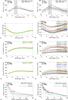 |
Fig. 5 VLTI/MIDI interferometry at 8–13 μm of RR Aql for the example of epoch A (stellar phase 0.58) and epoch I (stellar phase 2.75) . The panels show a) the flux; b) the visibility amplitude; c) the corresponding UD diameter; d) the corresponding Gaussian FWHM diameter as a function of wavelength. The gray shading indicates the wavelength region around 9.5 μm that is affected by atmospheric absorption. Panel e) shows the visibility amplitude as a function of spatial frequency for three averaged bandpasses of 8–9 μm, 10–11 μm, and 12–13 μm. The crosses with error bars denote the measured values. The solid lines indicate our best-fitting model, as described in Sect. 5. It consists of a combination of a dust-free dynamic model atmosphere representing the central star and a radiative transfer model representing the surrounding dust shell. The contributions of the stellar and dust components alone are indicated by the dotted and the dashed lines, respectively. |
Note that may slightly vary across the stellar disk, which is not taken into account here.
Acknowledgments
We gratefully acknowledge star observers around the world whose devoted observations provide active data support in the observations of the variable stars. We used the AAVSO International Database along with the AFOEV and SIMBAD databases, operated at the CDS, France. The authors would also like to acknowledge all who are involved in developing the publicly accessible MIDI data reduction software packages and tools EWS, MIA, and MyMidiGui, namely Walter Jaffe, Rainer Köhler, Christian Hummel, and others. This work is based on service mode observations made with the MIDI instrument, which is operated by ESO. We would like to thank the operating team at the Paranal Observatory for their careful execution of the observations.
References
- Alvarez, R., & Plez, B. 1998, A&A, 330, 1109 [NASA ADS] [Google Scholar]
- Andersen, A. C., Höfner, S., & Gautschy-Loidl, R. 2003, A&A, 400, 981 [NASA ADS] [CrossRef] [EDP Sciences] [Google Scholar]
- Begemann, B., Dorschner, J., Henning, T., et al. 1997, ApJ, 476, 199 [NASA ADS] [CrossRef] [Google Scholar]
- Benson, P. J., Little-Marenin, I. R., Woods, T. C., et al. 1990, ApJS, 74, 911 [NASA ADS] [CrossRef] [Google Scholar]
- Boboltz, D. A., & Wittkowski, M. 2005, ApJ, 618, 953 [NASA ADS] [CrossRef] [Google Scholar]
- Cohen, M., Walker, R. G., Carter, B., et al. 1999, AJ, 117, 1864 [NASA ADS] [CrossRef] [Google Scholar]
- Cotton, W. D., Perrin, G., & Lopez, B. 2008, A&A, 477, 853 [NASA ADS] [CrossRef] [EDP Sciences] [Google Scholar]
- Danchi, W. C., Bester, M., Degiacomi, C. G., Greenhill, L. J., & Townes, C. H. 1994, AJ, 107, 1469 [NASA ADS] [CrossRef] [Google Scholar]
- Diamond, P. J., Kemball, A. J., Junor, W., et al. 1994, ApJ, 430, L61 [NASA ADS] [CrossRef] [Google Scholar]
- Driebe, T., Hofmann, K., Ohnaka, K., et al. 2008, in The Power of Optical/IR Interferometry: Recent Scientific Results and 2nd Generation, ed. A. Richichi, F. Delplancke, F. Paresce, & A. Chelli (Berlin, Heidelberg, New York: Springer), 507 [Google Scholar]
- Fedele, D., Wittkowski, M., Paresce, F., et al. 2005, A&A, 431, 1019 [NASA ADS] [CrossRef] [EDP Sciences] [Google Scholar]
- Glindemann, A., Algomedo, J., Amestica, R., et al. 2003, in Proc. SPIE 4838, ed. W. A. Traub, 89 [Google Scholar]
- Guha Niyogi, S., Speck, A. K., & Onaka, T. 2011, ApJ, 733, 93 [NASA ADS] [CrossRef] [Google Scholar]
- Haniff, C. A., Scholz, M., & Tuthill, P. G. 1995, MNRAS, 276, 640 [NASA ADS] [CrossRef] [Google Scholar]
- Hofmann, K., Scholz, M., & Wood, P. R. 1998, A&A, 339, 846 [NASA ADS] [Google Scholar]
- Höfner, S. 2008, A&A, 491, L1 [NASA ADS] [CrossRef] [EDP Sciences] [Google Scholar]
- Höfner, S. 2011 [arXiv:1102.5268] [Google Scholar]
- Höfner, S., & Andersen, A. C. 2007, A&A, 465, L39 [NASA ADS] [CrossRef] [EDP Sciences] [Google Scholar]
- Ireland, M. J., & Scholz, M. 2006, MNRAS, 367, 1585 [NASA ADS] [CrossRef] [Google Scholar]
- Ireland, M. J., Scholz, M., Tuthill, P. G., & Wood, P. R. 2004a, MNRAS, 355, 444 [NASA ADS] [CrossRef] [Google Scholar]
- Ireland, M. J., Scholz, M., & Wood, P. R. 2004b, MNRAS, 352, 318 [NASA ADS] [CrossRef] [Google Scholar]
- Ireland, M. J., Scholz, M., & Wood, P. R. 2008, MNRAS, 391, 1994 [NASA ADS] [CrossRef] [Google Scholar]
- Koike, C., Kaito, C., Yamamoto, T., et al. 1995, Icarus, 114, 203 [NASA ADS] [CrossRef] [Google Scholar]
- Leinert, C., van Boekel, R., Waters, L. B. F. M., et al. 2004, A&A, 423, 537 [NASA ADS] [CrossRef] [EDP Sciences] [Google Scholar]
- Little-Marenin, I. R., & Little, S. J. 1990, AJ, 99, 1173 [NASA ADS] [CrossRef] [Google Scholar]
- Lorenz-Martins, S., & Pompeia, L. 2000, MNRAS, 315, 856 [NASA ADS] [CrossRef] [Google Scholar]
- Lopez, B., Danchi, W. C., Bester, M., et al. 1997, ApJ, 488, 807 [NASA ADS] [CrossRef] [Google Scholar]
- Matsuura, M., Barlow, M. J., Zijlstra, A. A., et al. 2009, MNRAS, 396, 918 [NASA ADS] [CrossRef] [Google Scholar]
- Millan-Gabet, R., Pedretti, E., Monnier, J. D., et al. 2005, ApJ, 620, 961 [NASA ADS] [CrossRef] [Google Scholar]
- Miyata, T., Kataza, H., Okamoto, Y., Onaka, T., & Yamashita, T. 2000, ApJ, 531, 917 [NASA ADS] [CrossRef] [Google Scholar]
- Molster, F. J., & Waters, L. B. F. M. 2003, in Astromineralogy, ed. T. K. Henning (Berlin, Verlag: Springer), 121 [Google Scholar]
- Monnier, J. D., Bester, M., Danchi, W. C., et al. 1997, ApJ, 481, 420 [NASA ADS] [CrossRef] [Google Scholar]
- Monnier, J. D., Geballe, T. R., & Danchi, W. C. 1998, ApJ, 502, 833 [NASA ADS] [CrossRef] [Google Scholar]
- Monnier, J. D., Danchi, W. C., Hale, D. S., et al. 2000, ApJ, 543, 861 [Google Scholar]
- Ohnaka, K. 2004, A&A, 424, 1011 [NASA ADS] [CrossRef] [EDP Sciences] [Google Scholar]
- Ohnaka, K., Bergeat, J., Driebe, T., et al. 2005, A&A, 429, 1057 [NASA ADS] [CrossRef] [EDP Sciences] [Google Scholar]
- Ohnaka, K., Driebe, T., Hofmann, K., et al. 2006, A&A, 445, 1015 [NASA ADS] [CrossRef] [EDP Sciences] [Google Scholar]
- Ohnaka, K., Driebe, T., Weigelt, G., & Wittkowski, M. 2007, A&A, 466, 1099 [NASA ADS] [CrossRef] [EDP Sciences] [Google Scholar]
- Ohnaka, K., Izumiura, H., Leinert, C., et al. 2008, A&A, 490, 173 [NASA ADS] [CrossRef] [EDP Sciences] [Google Scholar]
- Ossenkopf, V., Henning, T., & Mathis, J. S. 1992, A&A, 261, 567 [NASA ADS] [Google Scholar]
- Perrin, G., Coudé du Foresto, V., Ridgway, S. T., et al. 1999, A&A, 345, 221 [NASA ADS] [Google Scholar]
- Pojmanski, G., Pilecki, B., & Szczygiel, D. 2005, Acta Astron., 55, 275 [NASA ADS] [Google Scholar]
- Quirrenbach, A., Mozurkewich, D., Armstrong, J. T., et al. 1992, A&A, 259, L19 [NASA ADS] [Google Scholar]
- Ragland, S., Traub, W. A., Berger, J., et al. 2006, ApJ, 652, 650 [NASA ADS] [CrossRef] [Google Scholar]
- Samus, N. N., Durlevich, O. V., et al. 2004, VizieR Online Data Catalog, 2250 [Google Scholar]
- Tej, A., Lançon, A., Scholz, M., & Wood, P. R. 2003, A&A, 412, 481 [NASA ADS] [CrossRef] [EDP Sciences] [Google Scholar]
- Tevousjan, S., Abdeli, K., Weiner, J., Hale, D. D. S., & Townes, C. H. 2004, ApJ, 611, 466 [Google Scholar]
- Thompson, R. R., Creech-Eakman, M. J., & Akeson, R. L. 2002a, ApJ, 570, 373 [NASA ADS] [CrossRef] [Google Scholar]
- Thompson, R. R., Creech-Eakman, M. J., & van Belle, G. T. 2002b, ApJ, 577, 447 [NASA ADS] [CrossRef] [Google Scholar]
- van Belle, G. T., Dyck, H. M., Benson, J. A., & Lacasse, M. G. 1996, AJ, 112, 2147 [NASA ADS] [CrossRef] [Google Scholar]
- van Belle, G. T., Thompson, R. R., & Creech-Eakman, M. J. 2002, AJ, 124, 1706 [NASA ADS] [CrossRef] [Google Scholar]
- Vlemmings, W. H. T., & van Langevelde, H. J. 2007, A&A, 472, 547 [NASA ADS] [CrossRef] [EDP Sciences] [Google Scholar]
- Vlemmings, W. H. T., van Langevelde, H. J., Diamond, P. J., Habing, H. J., & Schilizzi, R. T. 2003, A&A, 407, 213 [NASA ADS] [CrossRef] [EDP Sciences] [Google Scholar]
- Weiner, J., Tatebe, K., Hale, D. D. S., et al. 2006, ApJ, 636, 1067 [NASA ADS] [CrossRef] [Google Scholar]
- Whitelock, P., Marang, F., & Feast, M. 2000, MNRAS, 319, 728 [NASA ADS] [CrossRef] [Google Scholar]
- Wittkowski, M., Boboltz, D. A., Ohnaka, K., Driebe, T., & Scholz, M. 2007, A&A, 470, 191 [NASA ADS] [CrossRef] [EDP Sciences] [Google Scholar]
- Wittkowski, M., Boboltz, D. A., Driebe, T., et al. 2008, A&A, 479, L21 [NASA ADS] [CrossRef] [EDP Sciences] [Google Scholar]
- Woitke, P. 2006, A&A, 460, L9 [NASA ADS] [CrossRef] [EDP Sciences] [Google Scholar]
- Woodruff, H. C., Eberhardt, M., Driebe, T., et al. 2004, A&A, 421, 703 [NASA ADS] [CrossRef] [EDP Sciences] [Google Scholar]
- Woodruff, H. C., Tuthill, P. G., Monnier, J. D., et al. 2008, ApJ, 673, 418 [NASA ADS] [CrossRef] [Google Scholar]
- Wyatt, S. P., & Cahn, J. H. 1983, ApJ, 275, 225 [NASA ADS] [CrossRef] [Google Scholar]
- Young, J. S., Baldwin, J. E., Boysen, R. C., et al. 2000a, MNRAS, 315, 635 [NASA ADS] [CrossRef] [Google Scholar]
- Young, J. S., Baldwin, J. E., Boysen, R. C., et al. 2000b, MNRAS, 318, 381 [NASA ADS] [CrossRef] [Google Scholar]
All Tables
Model simulations, comparing two models that differ in one or more parameters (marked by bold face).
All Figures
|
Fig. 1 Visual light curve of RR Aql based on data from the AAVSO and AFOEV databases as a function of Julian Date and stellar cycle/phase. The green arrows indicate the dates of our VLTI/MIDI observations. The blue arrows indicate the dates of our VLBA observations. Here, the full arrows denote observations of SiO maser emission and simple arrows observations of H2O maser emission. |
| In the text | |
|
Fig. 2 Calibrated RR Aql MIDI flux spectra as a function of wavelength. For clarity, the error bars are omitted in the plot. |
| In the text | |
|
Fig. 3 RR Aql flux spectrum as a function of wavelength from 2.4 μm to 40 μm (top). The lines represent the flux spectra from ISO-SWS observations covering wavelengths from 2.5 μm to ~240 μm (solid red thick line), IRAS-LRS observations covering ~7.7 μm to ~23 μm (dashed thin black line), and the mean of our N-band MIDI measurements (solid thin green line). Here, the vertical bars span the maximum and minimum values measured. The diamonds denote 2MASS measurements at 1.25 μm, 1.65 μm, and 2.2 μm. The solid black line indicates our atmosphere and dust shell model as explained in Sect. 5.2. The bottom plot shows an enlarged segment of the plot in the MIDI wavelength range of 8–13 μm. |
| In the text | |
|
Fig. 4 Calibrated RR Aql MIDI visibility amplitudes as a function of wavelength. (top left) Observations executed at projected baselines (Bp) < 20 m, (top right) 20 m < Bp < 35 m, (bottom left) 35 m < Bp < 50 m, and (bottom right) Bp > 50 m. |
| In the text | |
|
Fig. 6 Calibrated MIDI visibility amplitudes for different pulsation phases within the same cycle to investigate intracycle visibility variations. Each line represents a different pulsation phase within the same cycle and is computed as an average of data obtained at the respective phase ( ± 0.15) and observed at similar projected baseline length (Bp ± 10%) and position angle (PA ± 10%). The top panel shows the example of pulsation phases 0.45, 0.61, and 0.74 of cycle two observed with a projected baseline length of ~29 m and a position angle of ~70 deg. The bottom panel shows the example of pulsation phases 0.62, 0.75, and 0.83 of cycle two observed with a projected baseline length of ~16 m and a position angle of ~72 deg. The error bars are computed as the standard deviation of the averaged visibilities. |
| In the text | |
|
Fig. 7 As for Fig. 6, but for the same pulsation phase in consecutive pulsation cycles to investigate cycle-to-cycle visibility variations. The top panel shows the example of pulsation phase ~0.5 in three consecutive cycles observed with a projected baseline length of ~61 m and a position angle ~75 deg. The bottom panel shows the example of pulsation phase 0.5 in two consecutive cycles observed with a projected baseline length of ~29 m and a position angle ~70 deg. |
| In the text | |
|
Fig. 8 Calibrated MIDI flux spectrum for different pulsation phases within the same cycle to investigate intracycle photometry variations. Each line represents a different pulsation phase within the same cycle and is computed as an average of data obtained at the respective phase ( ± 0.15). The top panel shows the example of pulsation phases 0.58 and 0.85 of cycle zero. The bottom panel shows the examples of phases 0.53 and 0.76 of cycle one. The error bars are computed as the standard deviation of the averaged photometry curves. The gray shades denote zones that are affected by atmospheric absorption. |
| In the text | |
|
Fig. 9 As for Fig. 8, but for the same pulsation phase in consecutive pulsation cycles to investigate cycle-to-cycle photometry variations. The top panel shows the example of phase ~0.75 in cycles one and two. The bottom panel shows the example of phase ~0.85 of cycles zero and two. |
| In the text | |
|
Fig. 10 Simulation 1. Synthetic flux (top) and visibility amplitude (bottom) in the wavelength range 8–13 μm. The solid lines represent the global models, the dashed-dotted lines denote the unattenuated stellar contribution i.e. Vstar in Eq. (2), the dotted lines denote the attenuated stellar contribution, and the dashed lines denote the dust shell contributions. This simulation compares two models consisting of the same dust shell parameters but different model atmospheres, the post-maximum model atmosphere M21n (Φmodel = 0.10), and the minimum model atmosphere M23n (Φmodel = 0.30). The photospheric angular diameter is assumed to be larger at post-maximum phase than at minimum phase (8.5 mas compared to 7 mas). The projected baseline length is 60 m. For the exact model parameters, see Table 4. They describe variations around our best-fitting model for RR Aql. |
| In the text | |
|
Fig. 11 Simulation 2. Like simulation 1 in Fig. 10, but for the parameters of simulation 2 comparing a post-maximum atmosphere model and a minimum model as in simulation 1, but where the dust is also assumed to be closer to the star with larger optical depth at minimum phase and farther from the star with lower optical depth at post-maximum phase. |
| In the text | |
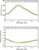 |
Fig. 12 Simulation 3. As for simulation 2 in Fig. 11, but where the atmosphere model is not varied. |
| In the text | |
|
Fig. 13 Simulation 3. As Fig. 12, but showing the visibility spectra for different projected baseline lengths of (from top to bottom) 40 m, 25 m, and 15 m. |
| In the text | |
|
Fig. 14 Simulation 4. Comparison of a model with a silicate shell only and a model that also includes an Al2O3 dust shell with lower optical depth. For the model parameters, see Table 4; For the description of the figure, see the caption of Fig. 10. |
| In the text | |
|
Fig. 5 VLTI/MIDI interferometry at 8–13 μm of RR Aql for the example of epoch A (stellar phase 0.58) and epoch I (stellar phase 2.75) . The panels show a) the flux; b) the visibility amplitude; c) the corresponding UD diameter; d) the corresponding Gaussian FWHM diameter as a function of wavelength. The gray shading indicates the wavelength region around 9.5 μm that is affected by atmospheric absorption. Panel e) shows the visibility amplitude as a function of spatial frequency for three averaged bandpasses of 8–9 μm, 10–11 μm, and 12–13 μm. The crosses with error bars denote the measured values. The solid lines indicate our best-fitting model, as described in Sect. 5. It consists of a combination of a dust-free dynamic model atmosphere representing the central star and a radiative transfer model representing the surrounding dust shell. The contributions of the stellar and dust components alone are indicated by the dotted and the dashed lines, respectively. |
| In the text | |
Current usage metrics show cumulative count of Article Views (full-text article views including HTML views, PDF and ePub downloads, according to the available data) and Abstracts Views on Vision4Press platform.
Data correspond to usage on the plateform after 2015. The current usage metrics is available 48-96 hours after online publication and is updated daily on week days.
Initial download of the metrics may take a while.