© ESO, 2011

1. Introduction

The objects now termed infrared dark clouds (IRDCs) were first identified by Perault et al. (1996) and Egan et al. (1998) in images of the Galactic plane made with the Infrared Space Observatory (ISO) and the Midcourse Space Experiment (MSX) satellite, respectively. IRDCs have significant extinctions even at 8 and 15 μm and are, thus, seen in silhouette against the bright, diffuse, mid-infrared Galactic emission. Millimeter and (sub)millimeter molecular studies reveal that some clumps within IRDCs have column densities of  >10²³ cm^-2, volume gas densities of n  >  10⁵ cm^-3, and temperatures T  <  20 K (e.g., Carey et al. 1998; Pillai et al. 2006a). Several studies suggest that IRDCs have the potential of harboring the earliest stages of massive star formation and indeed evidence for this is found toward distinct regions within them (Rathborne et al. 2005; Pillai et al. 2006b; Wang et al. 2006).

Pillai et al. (2006a) mapped the (J,K)  =  (1,1) and (2,2) inversion transitions of ammonia (NH₃) in the IRDC G11.11-0.12 with the Effelsberg 100 m telescope and found gas temperatures of the order of 15 K for several clumps within this cloud. The left panel of Fig. 1 shows an overview of the region. Furthermore, Pillai et al. (2006b) reported the detection of 6.7 GHz class II methanol (CH₃OH) and 22.2 GHz water (H₂O) masers in the IRDC core G11.11-0.12P1 (hereafter G11.11P1). Both CH₃OH and H₂O masers are known as tracers of massive star formation. They found that these masers were associated with a SCUBA dust continuum peak (P1; Carey et al. 2000) and ascribed the kinematics of the methanol masing spots to a maser amplification from a Keplerian disk.

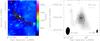Fig. 1 Left: SCUBA 850 μm (Carey et al. 2000) contours overlaid on the MIPSGAL 24 μm image of the IRDC G11.11-0.12. Right: PdBI 1.2 mm continuum emission (contours) of G11.11P1 overlaid on the 3.1 mm continuum emission (grey scale image). First contour and contour spacing for the 3.1 mm emission are 0.9 mJy beam-1 (3σ), the dotted contours show the negative emission (− 3σ); the synthesized beam (60  ×  31; PA = 176°) is shown in the bottom left corner. First contour and contour spacing for the 1.2 mm emission are 6.3 mJy beam-1 (3σ), the dashed contours show the negative emission (− 3σ); the synthesized beam (26  ×  11; PA = 176°) is shown in the bottom right corner. The filled triangle at RA = 18h10m2829, Dec = −19°22′305 and the filled square at RA = 18h10m2825, Dec = −19°22′3045 (J2000) indicate the water and (integrated emission) methanol masers, respectively, reported by Pillai et al. (2006b).

Open with DEXTER

Henning et al. (2010) observed this filamentary IRDC with the PACS (at 70, 100, and 160 μm) and the SPIRE (250, 350, and 500 μm) instruments onboard the Herschel Space Observatory, with resolutions in the range of  ~6″−40″. For G11.11P1, they obtain from a modified blackbody fit to the PACS data, a dust temperature of 24 K, a luminosity of 1346 L_⊙, and a mass of 240 M_⊙. Pillai et al. (2006a) and Leurini et al. (2007b) used a two-component model to fit single-dish observations of NH₃ and CH₃OH spectra, respectively, and derived temperatures of  ~15−18 K for the extended component (with size of  ~20″ corresponding to 0.35 pc) and  ~47−60 K for the inner component (with a size of  ~3″ corresponding to 0.05 pc).

Methanol, which is a slightly asymmetric top molecule, has been used to derive physical parameters such as the density and temperature of IRDCs (Leurini et al. 2007b), high-mass protostellar objects (e.g., Leurini et al. 2007a), and massive young stars (e.g., van der Tak et al. 2000), as well as low-mass protostellar systems (Kristensen et al. 2010). In particular, van der Tak et al. (2000) carried out a study toward 13 massive star-forming regions and found three types of CH₃OH abundance (X_CH3OH ≡ N_CH3OH/N_H2) profiles: X_CH3OH ~ 10^-9 for the coldest sources, from 10^-9 to 10^-7 for warmer sources, and 10^-7 for hot cores. CH₃OH has also been associated with outflows where the methanol abundance enhancements have been found to be a factor as large as 400−1000 (e.g., Bachiller et al. 1995; Garay et al. 2002; Kristensen et al. 2010).

In this paper, we present arcsecond-resolution millimeter continuum and line observations toward G11.11P1 to determine its physical and chemical structure. In Sect. 2, we describe our observations carried out with the IRAM Plateau de Bure Interferometer. In Sect. 3, we present continuum and line results together with the analysis. The discussion is presented in Sect. 4 and the summary is given in Sect. 5.

2. Observations and data reduction

2.1. IRAM PdBI observations

G11.11P1 was observed with the IRAM six element array Plateau de Bure Interferometer (PdBI; Guilloteau et al. 1992) in D and C configurations in 2005 and 2006, respectively.

During the 2006 observations, one antenna was equipped with the prototype New Generation Receiver. Because of a difference in the frequency scheme of this receiver, visibilities obtained in the image sideband in this antenna were discarded. The receivers were tuned single side-band at 3 mm and double side-band at 1 mm. The 3 mm receivers were centered at 96.64 GHz and the 1 mm receivers at 241.81 GHz (see Table 1). At 3 mm, the C³⁴S 2  →  1 line and the CH₃OH 2_k  →  1_k v_t = 0 lines were covered by using two correlator units of 80 MHz with a spectral resolution of 0.3125 MHz (0.97 km s^-1) and by two correlator units of 320 MHz. The latter, which are free of lines, were used to produce the continuum image with a total bandwith of  ~450 MHz. At 1 mm, the CH₃OH 5_k  →  4_k v_t = 0 lines were observed with two units of 160 MHz with a spectral resolution of 1.250 MHz (1.55 km s^-1). The remaining units of 80, 160, and 320 MHz were placed in such a way that a frequency range free of lines could be used to measure the continuum flux. The total bandwidth of both sidebands was  ~700 MHz.

The phase and amplitude were calibrated with observations of the object 1730-130. The bandpass calibration was done by observing 3C 273. MWC 349 was used as a primary flux calibrator of the 3 and 1 mm data (see Table 1). We estimate the final flux-density accuracy to be  ~5% and 10% for the 3 mm and 1 mm data, respectively. Continuum images were subtracted from the line data in the visibility plane. The combination of the C and D configurations provides angular scales in the ranges 18−126 (1 mm) and 44−325 (3 mm), i.e., providing information on spatial scales of 0.03−0.22 pc and 0.08−0.57 pc, respectively.

The calibration and data reduction were completed using the GILDAS package¹ at IRAM Grenoble. Images were created with natural weighting and CLEANed using the standard Högbom algorithm.

2.2. IRAM 30 m short-spacing observations

G11.11P1 was observed in the 2_k  →  1_k v_t = 0 (3 mm) and 5_k  →  4_k (1 mm) CH₃OH bands with the IRAM 30 m telescope. An area of 90″  ×  90″ was mapped with the SIS B100 receiver at 3 mm and 66″  ×  66″ with the HERA receiver (Schuster et al. 2004) at 1 mm with a bandwidth of  ~140 MHz. Sampling at 3 mm was of 15″, while at 1 mm it was of 6″. A conversion from antenna temperature to main-beam brightness temperature (T_MB) was performed by using a beam efficiency of 0.78 at 3 mm and 0.52 at 1 mm. The rms at 1 mm is 0.3 K and at 3 mm is 0.02 K. The data were reduced with the CLASS program, which is part of the GILDAS software package.

The 3 mm single-dish data are used to create short-spacing pseudo-visibilities; these are then merged with the interferometric observations. All data are imaged and deconvolved together. The processing was performed in GILDAS/MAPPING following standard procedures of the UV_SHORT task (see Rodríguez-Fernández et al. 2008² for details of the pseudo-visitbility technique). In Sect. 3.3, we present the result of recovering the short-spacing information for the 3 mm data.

Unfortunately, we were unable to merge the interferometric and single-dish observations for the 1 mm data because of the poor signal-to-noise ratio of the latter set of data. However, we used the 1 mm single-dish data in the following sections to help in the analysis and interpretation of this core.

3. Results and analysis

3.1. PdBI: Continuum emission

3.1.1. Morphology and core size

The right panel of Fig. 1 presents the continuum images at 1 and 3 mm of G11.11P1. At the resolution of both images, the emission is extended; the peak intensity positions coincide with each other and with the maser positions as well. The morphology at 3 mm resembles that previously imaged with the Berkeley-Illinois-Maryland-Association (BIMA) interferometer by Pillai et al. (2006b) with a slightly lower resolution (  ×  ).

In Table 2, we list the parameters of the continuum emission. Deconvolved sizes were obtained by fitting two-dimensional Gaussians to the continuum maps and yielding a core size of  ~0.16 pc  ×  0.08 pc with a PA 24° at 3 mm and  ~0.09 pc  ×  0.07 pc with a PA 165° at 1 mm. We assumed a kinematic distance of 3.6 kpc.

3.1.2. Mass

Assuming that the mm continuum is mainly due to optically thin dust emission, we estimate the gas mass, M_g, using the expression (Hildebrand 1983) 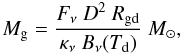(1)where F_ν is the observed integrated flux density in Jy, D is the distance, R_gd is the gas-to-dust mass ratio, κ_ν is the dust opacity coefficient, and B_ν(T_d) is the Planck function at the dust temperature (T_d). The 1 mm flux density was obtained by summing the 1 mm continuum emission above 3σ (>6 mJy beam^-1) level within a polygon encompassing the core, and the integrated flux density is  ~209 mJy. We assume a gas-to-dust mass ratio of 100, and adopt a κ_ν  =  1 cm² g^-1 (Ossenkopf & Henning 1994), at 1 mm, for an MRN (Mathis et al. 1977) graphite-silicate grain mixture with thick ice mantles, at a gas density of 10⁶ cm^-3. If we use T_d  =  60 K (Leurini et al. 2007b; Pillai et al. 2006a), a proper temperature for a region where methanol emission is produced, a mass of 13 M_⊙ at 1 mm is obtained for G11.11P1 (see Table 2). This is equivalent to adopting a dust opacity coefficient of k_ν = 0.1   (ν/10¹²   Hz)^β (Beckwith et al. 1990), which includes the gas contribution to the total mass for a R_gd = 100, with β  =  1.6. Given the uncertainties in the models of dust opacities and variation of the gas-to-dust ratio, β is within the errors comparable to the upper limit we obtain in Sect. 3.1.3.

Comparing the flux from the Bolocam Galactic Plane Survey (BGPS³; Aguirre et al. 2011) 1.1 mm with the PdBI 1.2 mm continuum flux, we find that the interferometric observations filter out about 75% of the emission.

To make a rough mass estimate of the core from the 3 mm data, all parameters remain the same as with the 1 mm data except for the flux density,  ~20 mJy, and κ_ν  =  0.2 cm² g^-1 (extrapolating from Table 1 Col. 9 in Ossenkopf & Henning 1994). We obtain a core mass of 37 M_⊙.

3.1.3. Density, temperature, and spectral indeces

For deeper insight into the source structure, we analyzed the 1 mm and 3 mm continuum data in the u-v domain avoiding the cleaning and u-v sampling effects. Figure 2 shows the averaged amplitudes averaged over a concentric annulus (from the continuum peak positions) versus deprojected u-v distance in units of wavelength. The amplitudes were averaged vectorially and the 3 mm u-v amplitudes in Jy were scaled by a factor of 15 to match the 1 mm visibilities. Error bars are 1σ statistical errors based on the standard deviation in the mean of the data points in the bin.

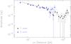Fig. 2 Continuum emission from G11.11P1 at 3.1 mm (filled triangles) and 1.2 mm (filled circles) in the Fourier domain. Amplitudes are averaged in bins of deprojected u-v distance from the continuum intensity peaks. The 3.1 mm u-v amplitudes have been scaled by a factor of 15. The straight solid line represents the least squares fit to the data. Error bars represent 1σ statistical errors based on the standard deviation in the mean of the data points in the bin.

Open with DEXTER

Since the index of the power law in u-v distance is related to the index of the power law in radial distance, r, following Looney et al. (2003), we can write F(r) ∝ r^{−(p + q)+1} → V(s) ∝ s^{(p + q)−3}, where F(r) is the flux density in the image domain, V(s) is the Fourier transform of the flux density, s is u-v distance and, p and q are the power-law indices of the density (n ∝ r^−p) and temperature structure (T ∝ r^−q), respectively.

The least squares fit (see Fig. 2) to both the 1 mm and 3 mm data yields a slope of −1.01  ±  0.02, corresponding to p + q  ~  2.0. Points starting at 40 kλ, which corresponds to an angular scale of  ~6″ (0.1 pc), were excluded from the fit because the signal-to-noise ratio gets very low. If the index q  =  0.4 (Goldreich & Kwan 1974), the density profile index is 1.6.

We estimate a mean volume gas density of the core (, where R is the core radius) of 7  ×  10⁵ cm^-3 using the mass derived from the dust observations at 1 mm (13 M_⊙), and the geometric mean of the deconvolved linear size as the core radius ( = 0.04 pc).

The scaling factor of 15 corresponds to a spectral index α  =  3.0  ±  0.4 and we thus obtain an opacity spectral index β  =  1.0  ±  0.4. The derived dust opacity index corresponds, taking the upper limit, to a “normal” interstellar dust material value. Nonetheless, if taking the lower limit, the dust opacity index decreases to a value that is usually found toward disks (e.g., Beckwith & Sargent 1991; Natta et al. 2004), which has been ascribed to grain growth. Alternatively, the presence of winds/outflows (see Sect. 4.2) could mimic a low value of β (Beuther et al. 2007). Here we adopt a β = 1.6 in the rest of the paper.

3.2. PdBI: molecular emission

Spectroscopic parameters of the detected C³⁴S 2  →  1 and CH₃OH 2_k  →  1_k and 5_k  →  4_k transitions toward G11.11P1 are listed in Table 3. The interferometric integrated intensity maps, overlaid on their corresponding continuum emission, along with sample spectra are presented in Figs. 3−5.

3.2.1. C³⁴S emission

The integrated intensity map of the C³⁴S 2  →  1 line, is shown in the top panel of Fig. 3. This emission is spatially coincident with the 3 mm continuum; moreover, some weaker emission (at 3σ level) extends along the E-W direction. Observed parameters toward the peak position in the integrated intensity map are presented in Table 4.

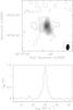Fig. 3 Top: contour image of the emission integrated under the C34S 2  →  1 line, in the velocity range from 22.4 to 37.9 km s-1, overlaid on the grey-scale 3.1 mm continuum emission of G11.11P1. First contour and contour spacing are 0.09 Jy beam-1 km s-1 (3σ), the dashed contours show the negative emission (− 3σ). The synthesized beam (60  ×  32; PA = 176°) is shown in the lower right corner. Bottom: spectrum of C34S 2  →  1 toward the peak position on the integrated intensity map at RA = 18h10m2824, Dec = −19°22′305 (J2000).

Open with DEXTER

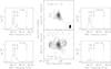Fig. 4 In greyscale, the 3.1 mm continuum emission of G11.11P1. Top middle: contour image of the CH3OH emission integrated under the line 21  →  11E. First contour and contour spacing are 0.66 Jy beam-1 km s-1 (3σ). The synthesized beam (60  ×  32; PA = 174°) is shown in the lower right corner. Bottom middle: contour image of the CH3OH emission integrated under the 2-1  →  1-1E, 20  →  10A, and 20  →  10E transition lines. First contour and contour spacing are 0.45 Jy beam-1 km s-1 (3σ). The dashed contours show the negative emission (− 3σ). We also show spectra at four different positions; positions are given in each inset in parenthesis in units of arcsec.

Open with DEXTER

Virial mass.

The virial mass of a core with a power-law density distribution is (MacLaren et al. 1988), where k₁ = (5−2p)/(3 − p), σ_v is the three-dimensional root-mean-square velocity related to the FWHM line width, ΔV, through , R is the core radius, and G is the gravitational constant. For p = 1.6 (see Sect. 3.1.3), the virial mass can be expressed as (2)A virial mass of  ~135 M_⊙ is calculated when using ΔV = 4.1   km   s^-1 (see Table 4) of the C³⁴S optically thin line and R  =  0.05 pc, which corresponds to the geometric mean of the deconvolved linear size.

Virial parameter.

The virial parameter (Bertoldi & McKee 1992) for a spherical cloud is defined as α_vir ≡ M_vir/M_tot, where M_tot is the total mass. If we assume that M_tot = M_g = 37   M_⊙, then α_vir = 3.6.

We note that the C³⁴S line width could be affected by unbound motions, e.g., outflows, partially broadening the line and thereby significantly increasing the virial mass estimate, in addition to the virial parameter.

Jeans mass.

Following Stahler & Palla (2005), we can calculate the Jeans mass (3)where a is the isothermal sound speed and ρ is the mass density. For n = 7  ×  10⁵ cm^-3 (see Sect. 3.1.3) and T  =  60 K, we obtain a Jeans mass of  ~1.8 M_⊙. We find a gas mass (M_g) to the Jeans mass (M_J) ratio larger than unity; other interferometric studies (Rathborne et al. 2008; Zhang et al. 2009) toward IRDCs also find that M_g/M_J > 1.

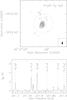Fig. 5 Top: contour image of the emission integrated under the 50  →  40A transition line, overlaid on the greyscale 1.2 mm continuum emission of G11.11P1. First contour and contour spacing are 0.16 Jy beam-1 km s-1 (3σ); the dashed contours show the negative emission (− 3σ). The synthesized beam (26  ×  11; PA = 174°) is shown in the lower right corner. The dotted circle indicates the interferometer primary beam (21″) at this frequency. Bottom: spectrum of CH3OH 5k  →  4k toward the position: RA = 18h10m2840, Dec = −19°22′319 (J2000). The HNCO 110,11  →  100,10 line (at 241 774.0320 MHz with Eu/k = 69.67 K and μ2S = 27.4590 D2) is shown as well. The “G” shows an artifact produced in the central channels of a correlator unit by the Gibbs effect.

Open with DEXTER

From our interferometric observations at 1 mm, and taking a flux density equal to the 3σ detection level, we derive a mass sensitivity limit of 0.4 M_⊙. Comparing this value with the Jeans mass, we note that our mass sensitivity limit is good enough to detect fragments of about the Jeans mass.

3.2.2. CH₃OH emission

Figure 4 shows the integrated intensity map of the CH₃OH 2_k  →  1_k quartet of lines (bottom middle). The emission exhibits three maxima: one is spatially coincident with the 1 and 3 mm continuum emission that peaks at (15, 0″), and the other two are located at (131, 0″) and (− 95, 22). We plot sample spectra at four different positions, including the three maxima and one position on the envelope (37, −73), to compare the line profiles, absolute line strengths, and the relative strengths among lines. The high excitation CH₃OH 2₁  →  1₁E transition that arises from a smaller region is also shown (top middle).

Line widths at and close to the three peak positions are on average  ~5 km s^-1 with line profiles showing red- and/or blueshifted “wings”, while in the outer parts of the envelope, e.g., at the (37, −73) position, the line width is narrower (~2 km s^-1; see spectra in Fig. 4).

In Fig. 5, we present the integrated intensity map of the strongest line CH₃OH 5₀  →  4₀A. The emission distribution is as extended as that of the 1 mm continuum and the CH₃OH 2₁  →  1₁E emissions.

Local thermodynamic equilibrium (LTE) analysis.

We derived the rotational temperatures and methanol column densities using the rotational diagram method (e.g., Cummins et al. 1986; Goldsmith & Langer 1999). Briefly, for an optically thin line, the column density in the upper level (N_u) can be written as N_u = 3kWg_u/(8π³νμ²S), where k is the Boltzmann constant, W is the integrated intensity of a line (), g_u the statistical weight, ν the frequency, S the line strength, and μ the dipole moment. Under LTE conditions, the population of each level follows a Boltzmann law at the gas temperature T by N_u = (N/Q)g_ue^−E_u/kT, where N is the total column density, Q the partition function, and E_u the energy of the upper level. We then obtain (4)Using Eq. (4), we plot  versus E_u/k (see Fig. 6) and perform a least squares fit for T and N taking into account both the CH₃OH 2_k  →  1_k and 5_k  →  4_k bands. The partition function of CH₃OH is (Turner 1991), where h is the Planck constant and A, B, and C are the rotation constants (CDMS; Müller et al. 2001, 2005). A Q = 1.23   T^1.5 relation was used in the calculations. The CH₃OH 5_k  →  4_k data were smoothed to the resolution of the 2_k  →  1_k data. The CH₃OH transition lines that were used in this fit are listed in Table 4.

	Fig. 6 Rotational diagram of CH3OH (2–1) and (5−4) transition lines toward the (15, 0″) position. The straight line is a least squares fit to the data corresponding to the rotational temperature and total column density indicated in the bottom left. Error bars are for 1σ uncertainties.
Open with DEXTER

To estimate the CH₃OH fractional abundance (relative to H₂), X_CH3OH, we calculate the beam-averaged H₂ column density, N_H2, following the expression 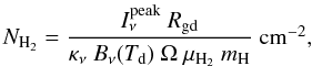(5)where is the peak intensity in Jy/beam, μ_H2  =  2.8 (Kauffmann et al. 2008) is the molecular weight per hydrogen molecule, and Ω = (πθ_minθ_maj)/(4ln2) is the beam solid angle of an elliptical Gaussian beam with minor and major axes θ_min and θ_maj, respectively.

We obtained a rotational temperature of 15 K and a CH₃OH column density, N_CH3OH, of 1.2  ×  10¹⁵ cm^-2 toward the (15, 0″) peak position. Since the lines are likely sub-thermally excited, we take a dust temperature T_d  =  60 K (see LVG analysis) and obtain a N_H2 = 4.6  ×  10²² cm^-2 (from our 1 mm continuum data convolved to the 3 mm data) and a X_CH3OH of 2.6  ×  10^-8.

At the (131, 0″) position, we obtain X_CH3OH = 3.7  ×  10^-9, when assuming that N_CH3OH = 2.9  ×  10¹⁴ cm^-2 and N_H2 = 7.7  ×  10²² cm^-2. A rotational temperature of 13 K was calculated. At the (− 95, 22) position, the values for the X_CH3OH, N_CH3OH, and N_H2 are 5.6  ×  10^-9, 3.8  ×  10¹⁴ cm^-2, and 6.8  ×  10²² cm^-2, respectively. For the (− 95, 22) peak, we fixed T = 15 K because of the low signal-to-noise ratio of one of the three lines used in the fit. For both peaks at (131, 0″) and (− 95, 22), N_CH3OH wa calculated from the 3 mm interferometric map only and N_H2 from the SCUBA 850 μm dust continuum; the interferometric observations were convolved to the SCUBA beam size (14″).

Large velocity gradient (LVG) analysis.

Leurini et al. (2004) found several ratios, from some CH₃OH-E transitions, to be calibration-independent tracers of density in the 1 and 3 mm bands. We used their LVG calculations and plotted the integrated intensity line ratios 5₀ → 4₀/5_-1 → 4_-1, 5₁ → 4₁/5_-1 → 4_-1, and 5₁ → 4₁/5₀ → 4₀, in a temperature-density (T − n) plane. In Fig. 7, the observed ratios, toward the (15,0″) position, are represented by the black dash-dotted line, blue solid line, and pink dashed line. The 2_k → 1_k quartet of lines in the 3 mm band were not used in the analysis because they are blended.

Given the results for CH₃OH column densities in the LTE analysis, the explored LVG models for the excitation of methanol run for temperatures in the range of 10−200 K, for densities 10⁵−10⁸ cm^-3, and for two CH₃OH column densities per line width 10¹⁴ and 10¹⁵ cm^-2/(km s^-1).

Fig. 7 Results of statistical equilibrium calculations for CH3OH-E. The 50 → 40/5-1 → 4-1 (black dash-dotted line), 51 → 41/5-1 → 4-1 (blue solid line), and 51 → 41/50 → 40 (pink dashed line) observed integrated intensity line ratios toward the (15, 0″) position on a logarithmic scale are shown as function of H2 density and temperature at NCH3OH/ΔV  =  1014 cm-2/(km s-1) (top) and NCH3OH/ΔV  =  1015 cm-2/(km s-1) (bottom).

Open with DEXTER

For an average line width of 4 km s^-1, this corresponds to N_{CH3OH − E} = 4  ×  10¹⁴ cm^-2 and 4  ×  10¹⁵ cm^-2, respectively. Depending on the column density, two possible solutions are found. At N_{CH3OH − E} = 4  ×  10¹⁴ cm^-2, the three integrated intensity line ratios intercept at T  =  17 K and n = 10⁷ cm^-3, whereas at N_{CH3OH − E} = 4  ×  10¹⁵ cm^-2, the interception is at T = 60 K and n = 2  ×  10⁶ cm^-3 (see Fig. 7). The methanol column density inferred in this case is consistent with the LTE analysis to within a factor of three, but the intensities in this model are one order of magnitude higher than the observed line intensities. In other words, to fit the observations with the N_{CH3OH − E} = 4  ×  10¹⁵ cm^-2 model, we need a beam filling factor of 0.1 resulting in a more compact source (with a size of 05 corresponding to 0.009 pc or 1800 AU), even smaller than the one modeled by Pillai et al. (2006a) and Leurini et al. (2007b).

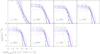	Fig. 8 Results of statistical equilibrium calculations for CH3OH-E. Observed integrated intensity line ratios are color-coded as in Fig. 7 and plotted on a logarithmic scale (along with their 1σ values) as a function of H2 density and NCH3OH/ΔV at different temperatures (10−70 K). The green dotted line represents the peak main brightness temperature of the 50 → 40E transition.
Open with DEXTER

To gain more insight into the possible T − n degeneracy, in Fig. 8, we show n versus N_CH3OH plots, at different temperatures (10−70 K), where the color-coding for the ratios (along with their 1σ values) are the same as in Fig. 7; in addition, we show in each panel the peak main beam brightness temperature of the 5₀ → 4₀E transition (green dotted line). The parameters obtained in the regions in the left side of the green dotted line imply beam filling factors greater than 1, which is not possible. In each panel, the areas of interest are those that lie in the right side of the green line and, at the same time, are delimited by the integrated intensity ratios (taking into account their 1σ values). We see that, for T in the range 30−70 K, the n remains constant up to N_CH3OH  ~ 4  ×  10¹⁴ cm^-2, while for very low T (=10 K) there is no solution.

Given our density estimate from the dust continuum, we regard the low T, high n solutions with a large filling factor as unlikely. Therefore, although we cannot strongly constrain the physical parameters of the gas emitting methanol from the LVG analysis because of the limited number of observed transitions, we can exclude the low temperature solution and place a lower limit on the kinetic temperature of the gas of 30 K. This result agrees with the detection of methanol maser from this region and with a previous measurement of T = 60 K from NH₃ observations. Therefore, we adopt T = 60 K as the kinetic temperature at the peak of the continuum emission.

3.3. PdBI+30 m: extended CH₃OH emission

A comparison of the interferometric data with the single-dish observations shows that only  ~30% of the CH₃OH 2_k  →  1_k measured with the 30 m telescope is imaged in the PdBI observations. The combined PdBI and 30 m telescope data recover almost 100% of the flux at the central (15, 0″) position. In Fig. 9, we show the resultant map after combining the CH₃OH 2_k →  1_k single-dish observations with the corresponding PdBI data. The methanol emission is already extended in the interferometric observations (mapping angular scales as large as 325) and confirmed to be so in the resultant merged map with the single-dish data. We note that the emission extends over a 1 pc scale in the merged map (see Fig. 9). Similarly, silicon monoxide (SiO) was found to be widespread over a 2 pc scale in the IRDC G035.39-00.33 (Jiménez-Serra et al. 2010). The 2₁ →  1₁E transition was not detected in the single-dish observations, which is expected since this emission does not appear to be extended in our interferometric data.

As for the 1mm data, the missing flux in the interferometric observations is  ~70%. In the 1 mm single-dish observations, two of the strongest transitions showed up, namely the 5_-1 →  4_-1E and the 5₀ →  4₀A lines. Both lines are above 3σ noise level at 6 of 144 observed positions.

How is the derivation of column densities and rotational temperatures affected by missing flux? Using the combined data at 3 mm only, the slope, i.e., the rotational temperature, in the rotational diagram is unaffected, within the errors, while CH₃OH column densities are higher by a factor of two.

4. Discussion

4.1. Properties of G11.11P1 relative to those of other cores

Despite our interferometric observations having sufficient sensitivity to resolve the Jeans mass (1.8 M_⊙) at 1 mm, the angular resolution (26  ×  11) is smaller than but very close to the Jeans length of 32 (0.05 pc). Therefore, it is difficult to ascertain whether G11.11P1 is fragmenting into condensations (referred to as substructures within the cores) as is often found when zooming into these cores (e.g., Zhang et al. 2009; Bontemps et al. 2010). If G11.11P1 were not to fragment, this would mean that it has already accumulated most of its mass that will go into the final star even though  ~75 % of the (dust) emission is filtered out by the interferometer. With higher angular resolution observations, it will be possible to determine whether either possibility is true.

The virial parameter of G11.11P1 obtained by Pillai et al. (2006a), from single-dish NH₃ and dust continuum (at 870 μm) observations, is unity on the scale of  ~0.9 pc. Although, in the present work, we find that M_vir is much higher than the M_g on the scale of  ~0.1 pc, which would indicate that gravity is not the dominant force (Bertoldi & McKee 1992). We caution, however, that the high value of the virial parameter (α_vir = 3.6) could be due to the missing flux in the interferometric data and to the virial mass being estimated from the C³⁴S line width, whose broadening is likely to be in part produced by outflows. Pillai et al. (2006b) reported an increase in line widths from 1.29 km s^-1 in the NH₃ (1, 1) line to 3.2 km s^-1 in the NH₃ (3, 3) data. The increase in NH₃ line width toward the higher (J,K) transitions suggest that star forming activity has a strong influence on the line width on smaller scales. The broad line width in the C³⁴S from PdBI is consistent with that notion.

On the basis of the SCUBA 870 μm column density, we estimated a surface density of Σ = 0.4 g cm^-2 for G11.11P1, which is close to the thresholds of 0.7−1.5 g cm^-2 (or 3320−7110 M_⊙ pc^-2) required to form stars of 10−200 M_⊙ (Krumholz & McKee 2008). We note that these authors were interested in clouds where no massive stars have yet formed, while G11.11P1 shows already signposts of star formation activity.

We calculated a density profile power-law index of 1.6 from interferometric observations at 1 and 3 mm; similar values, between 1.5 and 2, for cores in the IRDC G28.34+0.06, were reported by Zhang et al. (2009) also for embedded protostellar sources in the protocluster IRAS 05358+3543 (Beuther et al. 2007).

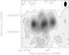Fig. 9 CH3OH 2k →  1kvt = 0 integrated intensity map combining PdBI and 30 m data. The emission is integrated over the 2-1 →  1-1E, 20 →  10A, and 20 →  10E transitions. First contour and contour spacing are 0.39 Jy beam-1 km s-1 (3σ), the dashed contours show the negative emission (− 3σ). The synthesized beam (62  ×  33; PA = 176°) is shown in the upper right corner. The dotted circle indicates the interferometer primary beam (52″).

Open with DEXTER

4.2. The disk/outflow system?

Pillai et al. (2006b) found a velocity gradient in the CH₃OH maser emission and explained it as the maser spots being located in a Keplerian disk. Interestingly, the spread of the maser components is in the north-south direction, which is perpendicular to the CH₃OH 2_k → 1_k emission that we propose originates by the presence of an outflow (in the east-west direction). The spread of the masing spots is translated into a radius of  ~450 AU for a hypothetical disk in G11.11P1. Cesaroni et al. (2006) reported that candidate disks in high-mass protostars have masses in the range 0.2−40 M_⊙ and radii of 500−10 000 AU. Our interferometric data set is capable of imaging the largest disk structures, but not those inferred in Pillai et al. (2006b).

G11.11P1 was cataloged by Cyganowski et al. (2008) as a “possible” massive young stellar object (YSO) outflow candidate. This categorization was based on the angular extent of the extended excess 4.5 μm emission, i.e., the extent of green emission in a three-color RGB image.

More evidence pointing to the presence of outflows comes from the non-Gaussian methanol line profiles (see Fig. 4 and Leurini et al. 2007b). In Fig. 10, we analyze the molecular emission in a position-velocity plot and note that there are “wings” of redshifted emission toward negative offsets and blueshifted emission toward positive offsets (see also Fig. 4). Moreover, we find a gradient of  ~4 km s^-1, in the east-west direction, for the CH₃OH 2_k →  1_k emission and speculate that it is due to an outflow(s)-cloud interaction. The C³⁴S 2  →  1 and CH₃OH 5_k  →  4_k lines are detected mainly toward the central peak/dust emission, and no velocity gradient is found.

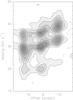Fig. 10 Position-velocity plot of the methanol 2k  →  1k lines, cutting along the PA = 96° on the map shown in the middle bottom panel of Fig. 4. We show the transitions: 2-1  →  1-1E, 20  →  10A, and 21  →  11E. The offset is measured in a positive direction toward east and from the pointing center of the observations. First contour is 0.018 in steps of 0.036 Jy beam-1, the dashed contours show the negative emission (− 0.018 Jy beam-1).

Open with DEXTER

Another possibility is that the CH₃OH 2_k  →  1_k emission is actually tracing a toroid (see Cesaroni et al. 2007) as in the interferometric observations of CH₃OH 6₀  →  5₀ toward the IRDC 18223-3 (Fallscheer et al. 2009). However, the gradient of the maser spots is orthogonal and not aligned with the gradient of the methanol emission that we present in Fig. 10.

4.3. CH₃OH abundances

Because methanol molecules can be sub-thermally excited (Bachiller et al. 1995), the temperatures derived from the rotational diagram are low (~15 K), even at the central peak where masers have been detected. To overcome this problem we used the LVG method and found that a higher temperature is more reliable.

Purely gas-phase model calculations predict that X_CH3OH is on the order of 10^-13−10^-10 (Garrod et al. 2006), which cannot reproduce the high values we report in this paper. Garrod et al. (2006) conclude that the production of methanol is carried out on the surfaces of dust grains followed by desorption into the gas. The X_CH3OH values in G11.P11 could then be produced by desorption of icy mantles on the dust grains.

As found in Sect. 3.2.2, the highest X_CH3OH in G11.11P1 is at the central position (X_CH3OH ~ 3  ×  10^-8), and is lower by more than one order of magnitude at the other two peaks, where X_CH3OH  ~  4−6  ×  10^-9; the same trend was also found by the LVG-modeling of single-dish data (Leurini et al. 2007b). Our abundances are enhanced relative to dark cloud values (X_CH3OH  ~  10^-10−10^-9; Friberg et al. 1988), also supporting the idea that methanol in G11.11P1 is forming mainly through non-thermal desorption by the presence of outflow(s).

5. Summary

We have performed continuum and line observations with the PdBI toward the IRDC core G11.11P1. Our main results can be summarized as follows:

• The analysis of the mm continuum maps provide a very detailedphysical structure of the core.

• Evidence that we have uncovered, i.e., “wings” in the CH₃OH 2_k  →  1_k spectra, and a CH₃OH abundance enhancement point to the presence of an outflow in the east-west direction.

• We have found a gradient of  ~4 km s^-1 for the CH₃OH 2_k  →  1_k emission, which we interpret as being produced by an outflow(s)-cloud interaction.

• Our fitting results have found an enhanced methanol fractional abundance (~3  ×  10^-8) at the central peak with respect to the other two maxima, where the methanol abundance is lower by about an order of magnitude (~4−6  ×  10^-9).

Acknowledgments

We acknowledge the IRAM staff at Pico Veleta and Plateau de Bure for carrying out the observations. L.G. thanks A. Castro-Carrizo and J. M. Winters for their help during the PdBI data reduction. We thank B. Parise for her evaluation of the manuscript and the referee for providing helpful comments and suggestions. L.G. was supported for this research through a stipend from the International Max Planck Research School (IMPRS) for Astronomy and Astrophysics at the Universities of Bonn and Cologne. T.P. acknowledges support from the Combined Array for Research in Millimeter-wave Astronomy (CARMA), which is supported by the National Science Foundation through grant AST 05-40399.

References

All Tables

All Figures

	Fig. 1 Left: SCUBA 850 μm (Carey et al. 2000) contours overlaid on the MIPSGAL 24 μm image of the IRDC G11.11-0.12. Right: PdBI 1.2 mm continuum emission (contours) of G11.11P1 overlaid on the 3.1 mm continuum emission (grey scale image). First contour and contour spacing for the 3.1 mm emission are 0.9 mJy beam-1 (3σ), the dotted contours show the negative emission (− 3σ); the synthesized beam (60  ×  31; PA = 176°) is shown in the bottom left corner. First contour and contour spacing for the 1.2 mm emission are 6.3 mJy beam-1 (3σ), the dashed contours show the negative emission (− 3σ); the synthesized beam (26  ×  11; PA = 176°) is shown in the bottom right corner. The filled triangle at RA = 18h10m2829, Dec = −19°22′305 and the filled square at RA = 18h10m2825, Dec = −19°22′3045 (J2000) indicate the water and (integrated emission) methanol masers, respectively, reported by Pillai et al. (2006b).
Open with DEXTER
In the text

	Fig. 2 Continuum emission from G11.11P1 at 3.1 mm (filled triangles) and 1.2 mm (filled circles) in the Fourier domain. Amplitudes are averaged in bins of deprojected u-v distance from the continuum intensity peaks. The 3.1 mm u-v amplitudes have been scaled by a factor of 15. The straight solid line represents the least squares fit to the data. Error bars represent 1σ statistical errors based on the standard deviation in the mean of the data points in the bin.
Open with DEXTER
In the text

	Fig. 3 Top: contour image of the emission integrated under the C34S 2  →  1 line, in the velocity range from 22.4 to 37.9 km s-1, overlaid on the grey-scale 3.1 mm continuum emission of G11.11P1. First contour and contour spacing are 0.09 Jy beam-1 km s-1 (3σ), the dashed contours show the negative emission (− 3σ). The synthesized beam (60  ×  32; PA = 176°) is shown in the lower right corner. Bottom: spectrum of C34S 2  →  1 toward the peak position on the integrated intensity map at RA = 18h10m2824, Dec = −19°22′305 (J2000).
Open with DEXTER
In the text

	Fig. 4 In greyscale, the 3.1 mm continuum emission of G11.11P1. Top middle: contour image of the CH3OH emission integrated under the line 21  →  11E. First contour and contour spacing are 0.66 Jy beam-1 km s-1 (3σ). The synthesized beam (60  ×  32; PA = 174°) is shown in the lower right corner. Bottom middle: contour image of the CH3OH emission integrated under the 2-1  →  1-1E, 20  →  10A, and 20  →  10E transition lines. First contour and contour spacing are 0.45 Jy beam-1 km s-1 (3σ). The dashed contours show the negative emission (− 3σ). We also show spectra at four different positions; positions are given in each inset in parenthesis in units of arcsec.
Open with DEXTER
In the text

	Fig. 5 Top: contour image of the emission integrated under the 50  →  40A transition line, overlaid on the greyscale 1.2 mm continuum emission of G11.11P1. First contour and contour spacing are 0.16 Jy beam-1 km s-1 (3σ); the dashed contours show the negative emission (− 3σ). The synthesized beam (26  ×  11; PA = 174°) is shown in the lower right corner. The dotted circle indicates the interferometer primary beam (21″) at this frequency. Bottom: spectrum of CH3OH 5k  →  4k toward the position: RA = 18h10m2840, Dec = −19°22′319 (J2000). The HNCO 110,11  →  100,10 line (at 241 774.0320 MHz with Eu/k = 69.67 K and μ2S = 27.4590 D2) is shown as well. The “G” shows an artifact produced in the central channels of a correlator unit by the Gibbs effect.
Open with DEXTER
In the text

	Fig. 6 Rotational diagram of CH3OH (2–1) and (5−4) transition lines toward the (15, 0″) position. The straight line is a least squares fit to the data corresponding to the rotational temperature and total column density indicated in the bottom left. Error bars are for 1σ uncertainties.
Open with DEXTER
In the text

	Fig. 7 Results of statistical equilibrium calculations for CH3OH-E. The 50 → 40/5-1 → 4-1 (black dash-dotted line), 51 → 41/5-1 → 4-1 (blue solid line), and 51 → 41/50 → 40 (pink dashed line) observed integrated intensity line ratios toward the (15, 0″) position on a logarithmic scale are shown as function of H2 density and temperature at NCH3OH/ΔV  =  1014 cm-2/(km s-1) (top) and NCH3OH/ΔV  =  1015 cm-2/(km s-1) (bottom).
Open with DEXTER
In the text

	Fig. 8 Results of statistical equilibrium calculations for CH3OH-E. Observed integrated intensity line ratios are color-coded as in Fig. 7 and plotted on a logarithmic scale (along with their 1σ values) as a function of H2 density and NCH3OH/ΔV at different temperatures (10−70 K). The green dotted line represents the peak main brightness temperature of the 50 → 40E transition.
Open with DEXTER
In the text

	Fig. 9 CH3OH 2k →  1kvt = 0 integrated intensity map combining PdBI and 30 m data. The emission is integrated over the 2-1 →  1-1E, 20 →  10A, and 20 →  10E transitions. First contour and contour spacing are 0.39 Jy beam-1 km s-1 (3σ), the dashed contours show the negative emission (− 3σ). The synthesized beam (62  ×  33; PA = 176°) is shown in the upper right corner. The dotted circle indicates the interferometer primary beam (52″).
Open with DEXTER
In the text

	Fig. 10 Position-velocity plot of the methanol 2k  →  1k lines, cutting along the PA = 96° on the map shown in the middle bottom panel of Fig. 4. We show the transitions: 2-1  →  1-1E, 20  →  10A, and 21  →  11E. The offset is measured in a positive direction toward east and from the pointing center of the observations. First contour is 0.018 in steps of 0.036 Jy beam-1, the dashed contours show the negative emission (− 0.018 Jy beam-1).
Open with DEXTER
In the text

References

- Aguirre, J. E., Ginsburg, A. G., Dunham, M. K., et al. 2011, ApJS, 192, 4 [NASA ADS] [CrossRef] [MathSciNet] [Google Scholar]
- Bachiller, R., Liechti, S., Walmsley, C. M., & Colomer, F. 1995, A&A, 295, L51 [NASA ADS] [Google Scholar]
- Beckwith, S. V. W., & Sargent, A. I. 1991, ApJ, 381, 250 [NASA ADS] [CrossRef] [Google Scholar]
- Beckwith, S. V. W., Sargent, A. I., Chini, R. S., & Guesten, R. 1990, AJ, 99, 924 [NASA ADS] [CrossRef] [Google Scholar]
- Bertoldi, F., & McKee, C. F. 1992, ApJ, 395, 140 [NASA ADS] [CrossRef] [Google Scholar]
- Beuther, H., Leurini, S., Schilke, P., et al. 2007, A&A, 466, 1065 [NASA ADS] [CrossRef] [EDP Sciences] [Google Scholar]
- Bontemps, S., Motte, F., Csengeri, T., & Schneider, N. 2010, A&A, 524, A18 [NASA ADS] [CrossRef] [EDP Sciences] [Google Scholar]
- Carey, S. J., Clark, F. O., Egan, M. P., et al. 1998, ApJ, 508, 721 [NASA ADS] [CrossRef] [Google Scholar]
- Carey, S. J., Feldman, P. A., Redman, R. O., et al. 2000, ApJ, 543, L157 [NASA ADS] [CrossRef] [Google Scholar]
- Cesaroni, R., Galli, D., Lodato, G., Walmsley, M., & Zhang, Q. 2006, Nature, 444, 703 [NASA ADS] [CrossRef] [PubMed] [Google Scholar]
- Cesaroni, R., Galli, D., Lodato, G., Walmsley, C. M., & Zhang, Q. 2007, Protostars and Planets V, 197 [Google Scholar]
- Cummins, S. E., Linke, R. A., & Thaddeus, P. 1986, ApJS, 60, 819 [NASA ADS] [CrossRef] [Google Scholar]
- Cyganowski, C. J., Whitney, B. A., Holden, E., et al. 2008, AJ, 136, 2391 [NASA ADS] [CrossRef] [Google Scholar]
- Egan, M. P., Shipman, R. F., Price, S. D., et al. 1998, ApJ, 494, L199 [NASA ADS] [CrossRef] [Google Scholar]
- Fallscheer, C., Beuther, H., Zhang, Q., Keto, E., & Sridharan, T. K. 2009, A&A, 504, 127 [NASA ADS] [CrossRef] [EDP Sciences] [Google Scholar]
- Friberg, P., Hjalmarson, A., Madden, S. C., & Irvine, W. M. 1988, A&A, 195, 281 [Google Scholar]
- Garay, G., Mardones, D., Rodríguez, L. F., Caselli, P., & Bourke, T. L. 2002, ApJ, 567, 980 [NASA ADS] [CrossRef] [Google Scholar]
- Garrod, R., Park, I. H., Caselli, P., & Herbst, E. 2006, Chemical Evolution of the Universe, Faraday Discussions, 133, 51 [Google Scholar]
- Goldreich, P., & Kwan, J. 1974, ApJ, 189, 441 [NASA ADS] [CrossRef] [Google Scholar]
- Goldsmith, P. F., & Langer, W. D. 1999, ApJ, 517, 209 [NASA ADS] [CrossRef] [Google Scholar]
- Guilloteau, S., Delannoy, J., Downes, D., et al. 1992, A&A, 262, 624 [NASA ADS] [Google Scholar]
- Henning, T., Linz, H., Krause, O., et al. 2010, A&A, 518, L95 [NASA ADS] [CrossRef] [EDP Sciences] [Google Scholar]
- Hildebrand, R. H. 1983, QJRAS, 24, 267 [NASA ADS] [Google Scholar]
- Jiménez-Serra, I., Caselli, P., Tan, J. C., et al. 2010, MNRAS, 406, 187 [NASA ADS] [CrossRef] [Google Scholar]
- Kauffmann, J., Bertoldi, F., Bourke, T. L., Evans, II, N. J., & Lee, C. W. 2008, A&A, 487, 993 [NASA ADS] [CrossRef] [EDP Sciences] [Google Scholar]
- Kristensen, L. E., van Dishoeck, E. F., van Kempen, T. A., et al. 2010, A&A, 516, A57 [NASA ADS] [CrossRef] [EDP Sciences] [Google Scholar]
- Krumholz, M. R., & McKee, C. F. 2008, Nature, 451, 1082 [NASA ADS] [CrossRef] [PubMed] [Google Scholar]
- Leurini, S., Schilke, P., Menten, K. M., et al. 2004, A&A, 422, 573 [NASA ADS] [CrossRef] [EDP Sciences] [Google Scholar]
- Leurini, S., Beuther, H., Schilke, P., et al. 2007a, A&A, 475, 925 [NASA ADS] [CrossRef] [EDP Sciences] [Google Scholar]
- Leurini, S., Schilke, P., Wyrowski, F., & Menten, K. M. 2007b, A&A, 466, 215 [NASA ADS] [CrossRef] [EDP Sciences] [Google Scholar]
- Looney, L. W., Mundy, L. G., & Welch, W. J. 2003, ApJ, 592, 255 [NASA ADS] [CrossRef] [Google Scholar]
- MacLaren, I., Richardson, K. M., & Wolfendale, A. W. 1988, ApJ, 333, 821 [NASA ADS] [CrossRef] [Google Scholar]
- Mathis, J. S., Rumpl, W., & Nordsieck, K. H. 1977, ApJ, 217, 425 [NASA ADS] [CrossRef] [Google Scholar]
- Müller, H. S. P., Thorwirth, S., Roth, D. A., & Winnewisser, G. 2001, A&A, 370, L49 [NASA ADS] [CrossRef] [EDP Sciences] [Google Scholar]
- Müller, H. S. P., Schlöder, F., Stutzki, J., & Winnewisser, G. 2005, J. Mol. Struct., 742, 215 [NASA ADS] [CrossRef] [Google Scholar]
- Natta, A., Testi, L., Neri, R., Shepherd, D. S., & Wilner, D. J. 2004, A&A, 416, 179 [NASA ADS] [CrossRef] [EDP Sciences] [Google Scholar]
- Ossenkopf, V., & Henning, T. 1994, A&A, 291, 943 [NASA ADS] [Google Scholar]
- Perault, M., Omont, A., Simon, G., et al. 1996, A&A, 315, L165 [NASA ADS] [Google Scholar]
- Pillai, T., Wyrowski, F., Carey, S. J., & Menten, K. M. 2006a, A&A, 450, 569 [NASA ADS] [CrossRef] [EDP Sciences] [Google Scholar]
- Pillai, T., Wyrowski, F., Menten, K. M., & Krügel, E. 2006b, A&A, 447, 929 [NASA ADS] [CrossRef] [EDP Sciences] [Google Scholar]
- Rathborne, J. M., Jackson, J. M., Chambers, E. T., et al. 2005, ApJ, 630, L181 [NASA ADS] [CrossRef] [Google Scholar]
- Rathborne, J. M., Jackson, J. M., Zhang, Q., & Simon, R. 2008, ApJ, 689, 1141 [NASA ADS] [CrossRef] [Google Scholar]
- Schuster, K., Boucher, C., Brunswig, W., et al. 2004, A&A, 423, 1171 [NASA ADS] [CrossRef] [EDP Sciences] [Google Scholar]
- Stahler, S. W., & Palla, F. 2005, The Formation of Stars (Wiley) [Google Scholar]
- Turner, B. E. 1991, ApJS, 76, 617 [NASA ADS] [CrossRef] [Google Scholar]
- van der Tak, F. F. S., van Dishoeck, E. F., & Caselli, P. 2000, A&A, 361, 327 [NASA ADS] [Google Scholar]
- Wang, Y., Zhang, Q., Rathborne, J. M., Jackson, J., & Wu, Y. 2006, ApJ, 651, L125 [NASA ADS] [CrossRef] [Google Scholar]
- Zhang, Q., Wang, Y., Pillai, T., & Rathborne, J. 2009, ApJ, 696, 268 [NASA ADS] [CrossRef] [Google Scholar]