| Issue |
A&A
Volume 527, March 2011
|
|
|---|---|---|
| Article Number | A145 | |
| Number of page(s) | 34 | |
| Section | Interstellar and circumstellar matter | |
| DOI | https://doi.org/10.1051/0004-6361/201015733 | |
| Published online | 14 February 2011 | |
The end of star formation in Chamaeleon I?
A LABOCA census of starless and protostellar cores ⋆,⋆⋆,⋆⋆⋆
1
Max-Planck Institut für Radioastronomie,
Auf dem Hügel 69,
53121
Bonn,
Germany
e-mail: This email address is being protected from spambots. You need JavaScript enabled to view it.
2
Laboratoire AIM, CEA/DSM-CNRS-Université Paris Diderot,
IRFU/Service d’Astrophysique, CEA Saclay, 91191
Gif-sur-Yvette,
France
3
School of Physics, University of Exeter,
Stocker Road,
Exeter
EX4 4QL,
UK
4
Centre for Star and Planet Formation, Natural History Museum of
Denmark, University of Copenhagen, Øster Voldgade 5–7, 1350
Copenhagen K.,
Denmark
5
Université de Bordeaux, Laboratoire d’Astrophysique de Bordeaux,
CNRS/INSU, UMR 5804, BP
89, 33271
Floirac Cedex,
France
Received:
10
September
2010
Accepted:
17
December
2010
Abstract
Context. Chamaeleon I is the most active region in terms of star formation in the Chamaeleon molecular cloud complex. Although it is one of the nearest low-mass star forming regions, its population of prestellar and protostellar cores is not known and a controversy exists concerning its history of star formation.
Aims. Our goal is to search for prestellar and protostellar cores and characterize the earliest stages of star formation in this cloud.
Methods. We used the bolometer array LABOCA at the APEX telescope to map the cloud in dust continuum emission at 870 μm with a high sensitivity. This deep, unbiased survey was performed based on an extinction map derived from 2MASS data. The 870 μm map is compared with the extinction map and C18O observations, and decomposed with a multiresolution algorithm. The extracted sources are analysed by carefully taking into account the spatial filtering inherent in the data reduction process. A search for associations with young stellar objects is performed using Spitzer data and the SIMBAD database.
Results. Most of the detected 870 μm emission is distributed in five filaments. We identify 59 starless cores, one candidate first hydrostatic core, and 21 sources associated with more evolved young stellar objects. The estimated 90% completeness limit of our survey is 0.22 M⊙ for the starless cores. The latter are only found above a visual extinction threshold of 5 mag. They are less dense than those detected in other nearby molecular clouds by a factor of a few on average, maybe because of the better sensitivity of our survey. The core mass distribution is consistent with the IMF at the high-mass end but is overpopulated at the low-mass end. In addition, at most 17% of the cores have a mass larger than the critical Bonnor-Ebert mass. Both results suggest that a large fraction of the starless cores may not be prestellar in nature. Based on the census of prestellar cores, Class 0 protostars, and more evolved young stellar objects, we conclude that the star formation rate has decreased with time in this cloud.
Conclusions. The low fraction of candidate prestellar cores among the population of starless cores, the small number of Class 0 protostars, the high global star formation efficiency, the decrease of the star formation rate with time, and the low mass per unit length of the detected filaments all suggest that we may be witnessing the end of the star formation process in Chamaeleon I.
Key words: stars: formation / ISM: individual objects: Chamaeleon I / ISM: structure / evolution / dust, extinction / stars: protostars
Based on observations carried out with the Atacama Pathfinder Experiment telescope (APEX). APEX is a collaboration between the Max-Planck Institut für Radioastronomie, the European Southern Observatory, and the Onsala Space Observatory.
Appendices are only available in electronic form at http://www.aanda.org
Table 2 is also available and FITS files of Fig. 2 are only available in electronic form at the CDS via anonymous ftp to cdsarc.u-strasbg.fr (130.79.128.5) or via http://cdsarc.u-strasbg.fr/viz-bin/qcat?J/A+A/527/A145
© ESO, 2011
1. Introduction
Large-scale, unbiased surveys in dust continuum emission have greatly improved our knowledge of the process of star formation in nearby, star-forming molecular clouds. During the past decade, (sub)mm dust continuum surveys established a close relationship between the prestellar core mass function (CMF) and the stellar initial mass function (IMF), suggesting that the IMF is already set at the early stage of cloud fragmentation (e.g. Motte et al. 1998; Testi & Sargent 1998; Johnstone et al. 2000). In these submm surveys, prestellar cores are found only above a visual extinction of 5–7 mag, suggesting the existence of an extinction threshold for star formation to occur (see, e.g., Johnstone et al. 2004; Enoch et al. 2006; Kirk et al. 2006; but also Onishi et al. 1998, based on molecular line observations).
In the mid-infrared range, five of these nearby molecular clouds – Chamaeleon II, Lupus, Perseus, Serpens, and Ophiuchus – were mapped with good angular resolution and high sensitivity with the Spitzer satellite in the frame of the c2d legacy project (From molecular cores to planet forming disks, see Evans et al. 2009). This extensive project produced a deep census of young stellar objects. It delivered star formation efficiencies ranging from 3 to 6% and Evans et al. (2009) estimate that these efficiencies could reach 15–30% if star formation continues at current rates in these clouds. Star formation is found to be slow compared to the free-fall time and highly concentrated to regions of high extinction (Evans et al. 2009), consistent with the threshold mentioned above.
Recently, the far-infrared/submm Herschel Space Observatory revealed an impressive network of parsec-scale filamentary structures in nearby molecular clouds in the frame of the Gould Belt Survey (André et al. 2010a). This survey greatly increases the statistics of prestellar cores and confirms the close relationship between the CMF and the IMF. In the Aquila molecular cloud, several hundreds of prestellar cores are identified, and André et al. (2010a) show that most of these prestellar cores are located in supercritical filaments. They confirm the existence of an extinction threshold for star formation at AV ~ 7 mag and propose that it may naturally come from the conditions required for a filament to become gravitationally unstable, collapse, and fragment into prestellar cores (see also André et al. 2010b). This finding will be further investigated in the frame of this Herschel survey, but it can also be partly tested in other nearby clouds in the submm range, thanks to the advent of very sensitive cameras like LABOCA at the Atacama Pathfinder Experiment telescope (APEX).
Chamaeleon I (Cha I) is one of the nearest, low-mass star forming regions in the southern sky (150–160 pc, Whittet et al. 1997; Knude & Høg 1998, see Appendix B.1 for more details). Together with Cha II and III, it belongs to the Chamaeleon cloud complex whose population of T-Tauri stars has been well studied (see Luhman 2008, and references therein). Cha I contains nearly one order of magnitude more young stars than Cha II, while Cha III does not have any. Surveys performed in CO and its isotopologues showed that Cha I contains a larger fraction of dense gas than Cha II and III although the latter are somewhat more massive (Boulanger et al. 1998; Mizuno et al. 1999, 2001). Finally, several indications of jets and outflows were found in Cha I (Mattila et al. 1989; Gómez et al. 2004; Wang & Henning 2006; Belloche et al. 2006). Only three Herbig-Haro objects are known in Cha II and none has been found in Cha III (Schwartz 1977). Cha I is therefore much more actively forming stars than Cha II and III.
A controversy exists, however, concerning the history of star formation in Cha I. Based on the H-R diagram of the young stellar population known at that time (47 members with known spectral type), Palla & Stahler (2000) conclude that star formation in Cha I began within the last 7 Myr and that its rate steadily increased until recently. They find similar results in several other clouds and draw the general conclusion that star formation in nearby associations and clusters started slowly some 10 Myr ago and accelerated until the present epoch. They speculate that this acceleration arises from contraction of the parent molecular cloud and results from star formation being a critical phenomenon occuring above some threshold density. However, based on a larger sample of known members, Luhman (2007) recently came to the conclusion that star formation began 3–6 Myr ago in Cha I and has continued to the present time at a declining rate. Since little is known about the earliest stages of star formation in Cha I, investigating whether there is presently a population of condensations that are prestellar, i.e. bound to form stars, should provide strong constraints on these two competing scenarii for the star formation history in Cha I.
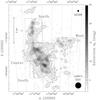 |
Fig. 1 Extinction map of Cha I derived from 2MASS in radio projection. The projection center is at (α,δ)J2000 = (11h01m24s, −77°15′00″). The contours start at AV = 3 mag and increase by step of 3 mag. The dotted lines are lines of constant right ascension. The angular resolution of the map (HPBW = 3′) is shown in the upper right corner. The four fields selected for mapping with LABOCA are delimited with dashed lines and their center is marked with a black cross. The white plus symbols in fields Cha-Center and Cha-North mark the positions of the dense cores Cha-MMS1 and Cha-MMS2, respectively, detected in dust continuum emission at 1.3 mm with the SEST (Reipurth et al. 1996). The field of view of LABOCA is displayed in the lower right corner. |
To unveil the present status of the earliest stages of star formation in Cha I, we carried out a deep, unbiased dust continuum survey of this cloud at 870 μm with the bolometer array LABOCA at APEX. The observations and data reduction are described in Sects. 2 and 3, respectively. The maps are presented in Sect. 4. Section 5 explains the source extraction and the sources are analysed in Sect. 6. The implications are discussed in Sect. 7. Section 8 gives a summary of our results and conclusions.
2. Observations
2.1. 870 μm continuum observations with APEX
The region of Cha I with a visual extinction higher than 3 mag was selected on the basis
of an extinction map derived from 2MASS1 (see
Sect. 2.2). It was divided into four contiguous
fields labeled Cha-North, Cha-Center, Cha-South, and Cha-West with a total angular area of
1.6 deg2 (see Fig. 1). The four fields
were mapped in continuum emission with the Large APEX BOlometer CAmera (LABOCA, Siringo et al. 2009) operating with about 250 working
pixels in the 870 μm atmospheric window at the APEX 12 m submillimeter
telescope (Güsten et al. 2006). The central
frequency of LABOCA is 345 GHz and its angular resolution is 19.2″
(HPBW). The observations were carried out for a total of 43 h in August,
October, November, and December 2007 (fields Cha-Center and Cha-South) and for 41 h in May
2008 (fields Cha-North and Cha-West), under excellent
( ) to good
(
) to good
( ) atmospheric conditions.
The sky opacity was measured every 1 to 2 h with skydips. The focus was optimised on Mars,
Saturn, or Venus at least once per day/night. The pointing of the telescope was checked
every hour on the nearby quasar PKS1057-79and was found to be accurate within 1.9″ for the
2007 data and 2.8″ for the 2008 data (rms). The calibration was performed with the
secondary calibrators IRAS 13134-6264, IRAS 16293-2422, V883 Ori, or NGC 2071 that were
observed every 1 to 2 h (see Table A.1 of Siringo et al.
2009). Measurements on the primary calibrator Mars were also used.
) atmospheric conditions.
The sky opacity was measured every 1 to 2 h with skydips. The focus was optimised on Mars,
Saturn, or Venus at least once per day/night. The pointing of the telescope was checked
every hour on the nearby quasar PKS1057-79and was found to be accurate within 1.9″ for the
2007 data and 2.8″ for the 2008 data (rms). The calibration was performed with the
secondary calibrators IRAS 13134-6264, IRAS 16293-2422, V883 Ori, or NGC 2071 that were
observed every 1 to 2 h (see Table A.1 of Siringo et al.
2009). Measurements on the primary calibrator Mars were also used.
The observations were performed on the fly, alternately with rectangular (“OTF”) and spiral scanning patterns (see Sect. 8 of Siringo et al. 2009). The OTF maps were alternately scanned in right ascension and declination, with a random position angle between −12° and +12° to improve the sampling and reduce striping effects. The “spiral” maps were obtained using rasters of spirals (see Sect. 3.1 for the parameters), with a random offset around the field center (within ± 30″ in each direction) to also improve the sampling.
2.2. Extinction map from 2MASS
We derived an extinction map toward Cha I from the publicly available 2MASS point source catalog (see Fig. 1). We selected all sources detected in either both J and H, or both H and K, or in all three bands. Before computing the extinction map, 223 young stellar objects (YSOs) that are known members of Cha I (see Table 1 of Luhman 2008) were removed from the sample. The extinction was calculated from the average reddening of stars inside the elements of resolution of the map using the method described in Schneider et al. (2011) that is adapted from Lada et al. (1994), Lombardi & Alves (2001), and Cambrésy et al. (2002). The extinction toward each star is obtained from the uncertainty-weighted combination of the [J − H] and [H − K] colors. The assumed average intrinsic colors are [J − H ] 0 = 0.45 ± 0.15, and [H − K ] 0 = 0.12 ± 0.05. These are derived from the typical dispersions for a population of galactic stars as measured using simulations with the Besançon stellar population model (Robin et al. 2003)2. The infrared color excess was converted to visual extinction assuming the standard extinction law of Rieke & Lebofsky (1985), with a ratio of total to selective extinction RV = 3.1 (see Appendix B.3). In addition, we use the Besançon galactic model to derive the predicted density of foreground stars in the 2MASS bands. For the distance and the direction of the Chameleon clouds, it is found to be less than 0.01 star per arcmin2. Therefore it is negligible and no filtering for foreground stars is applied.
A Gaussian weight function for the local average of the individual extinctions defines the resolution of the final map, with a FWHM of 3′ and a pixel size of 1.5′. The FWHM is chosen so that most pixels (97%) with AV < 6 mag have at least 10 stars within a radius equal to FWHM / 2. Most pixels (96%) between 6 and 9 mag and between 9 and 13 mag have at least 4 and 3 stars, respectively. All pixels above 15 mag have between 2 and 4 stars. Only five pixels have no background star within FWHM / 2. Their extinction value is solely estimated from the stars located between FWHM / 2 and the truncation radius (1.3 FWHM), which means a small local loss of resolution. Two of these pixels are located within the AV = 12 mag contour of the Cha-MMS1 region.
The typical rms noise level in the outer parts of the map is 0.4 mag, i.e. a 3σ detection level of 1.2 mag for an FWHM of 3′. This rms noise level is however expected to increase towards the higher-extinction regions because of the decreasing number of stars per element of resolution.
Our map looks very similar to the extinction map of Kainulainen et al. (2006) in terms of structure and sensitivity. Their map was also based on 2MASS data and a similar method was used to compute the extinction. The main differences are that they chose a higher angular resolution (2′) and used only the 2MASS sources with a signal-to-noise ratio larger than 10 in J, H, and K, at the cost of a few dozens of pixels being empty due to the lack of background stars. The extinction maps of Cambrésy et al. (1997) and Cambrésy (1999), based on star counts in the J and R bands, respectively, are more sensitive in the low-extinction regions than our map, but they miss the high-extinction regions (see also discussion in Cambrésy et al. 2002).
2.3. Archival C18O 1–0 observations with SEST
The eastern part of Cha I was mapped with the Swedish ESO Submillimeter Telescope (SEST) in the C18O 1–0 line by Haikala et al. (2005). The angular resolution is 45″ but the map is highly undersampled since the observations were done with a step of 1′. The median rms noise level is 0.1 K for a channel width of 43 kHz (0.12 km s-1), but occasionally goes up to 0.22 K at certain positions. We retrieved the publicly available FITS data cube from the AA website. We reprojected the cube from B1950 to J2000 equatorial coordinates in radio projection with a projection center at (α,δ)J2000 = (11h01m24s, −77°15′00″). We applied a velocity correction of +0.25 km s-1 to all spectra (as recommended by L. Haikala, priv. comm.).
3. LABOCA data reduction
3.1. Reduction method
The LABOCA data were reduced with the BoA software3 following the procedures described in Sect. 10.2 of Siringo et al. (2009) and Sect. 3.1 of Schuller et al. (2009). The removal of the correlated noise was done with the median noise method applied to all pixels with 5 iterations and a relative gain of 0.9. Subsequently, the correlated noise computed separately for each group of pixels belonging to the same amplifier box was removed (BoA function correlbox with 3 iterations and a relative gain of 0.95), as well as the correlated noise computed separately for each group of pixels connected to the same read-out cable (BoA function correlgroup with 3 iterations and a relative gain of 0.8).
The power at frequencies below 0.1 Hz in the Fourier domain was partially filtered out to reduce the 1 / f noise. It was replaced with the average power measured between 0.1 and 0.15 Hz (BoA function flattenFreq). Since the OTF scans were performed with a mapping speed of 2 arcmin s-1, the frequency 0.1 Hz corresponds to an angular scale of 20′. The analysis is different for the spiral scans. An individual spiral subscan had a duration of 40 s, an angular speed of 60 deg s-1, and a radius linearly increasing from 2′ to 3′. A frequency of 0.1 Hz corresponds to 10 s, i.e. about 1.7 turns. As a result, the typical angular scale associated with the cutoff frequency of 0.1 Hz is the spiral “diameter” which varied between 4.5′ and 6′. In addition to this low-frequency “flattening”, a first order baseline was subtracted scan-wise. The gridding was done with a cell size of 6.1″ and the map was smoothed with a Gaussian kernel of size 9″ (FWHM). The angular resolution of the final map is 21.2″ (HPBW) and the rms noise level is 12 mJy/21.2″-beam (see Sect. 4.1).
This whole process was performed 21 times in an iterative way. The pixel values in the map produced at iteration 0 (resp. 1) were set to zero below a signal-to-noise ratio of 4. The location of the remaining signal was used as an astronomical source model to mask the raw data at the start of iteration 1 (resp. 2). The mask was removed at the end of iteration 1 (resp. 2) to compute the reduced map. Iterations 3 to 20 were performed differently: the pixel values of the map resulting from the previous iteration were set to zero below a signal-to-noise ratio of 2.5. The remaining signal was subtracted from the raw data before reduction and added back after reduction. Masking or subtracting the significant astronomical signal found after one iteration permits to protect these regions at the next iteration when removing the correlated signal, flattening the low-frequency part of the power spectrum, and subtracting the first-order baseline. In this way, negative bowls around strong sources are much reduced and more extended emission can be recovered.
3.2. Spatial filtering and convergence
Data reduction features dealing with spatial filtering and convergence are analysed in detail in Appendix A. Here we give a brief summary. The correlated noise removal severely limits the extent of the 870 μm emission that can be recovered (see Fig. A.1). Elongated structures are better recovered than circular ones (see Table A.1). The recovery of extended structures is improved by increasing the number of iterations of the data reduction. With 21 iterations, convergence is reached for most relevant structures (see Figs. A.2 and A.3).
4. Basic results
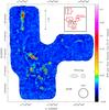 |
Fig. 2 870 μm continuum emission map of Cha I obtained with LABOCA at APEX. The projection type and center are the same as in Fig. 1. The contour levels are a, 2a, 4a, 8a, 16a, and 32a, with a = 48 mJy/21.2″-beam, i.e. about 4 times the rms noise level. The flux density color scale is shown on the right. The field of view of LABOCA (10.7′) and the angular resolution of the map (HPBW = 21.2″) are shown in the lower right corner. The typical sizes above which the filtering due to the data reduction becomes significant in terms of peak flux density are also displayed, for weak (<150 mJy/beam) and strong (>150 mJy/beam) sources with small and large symbols, respectively, and for elliptical sources with aspect ratio 2.5 and circular sources with ellipses and circles, respectively (see Appendix A.1 and Col. 2 of Table A.1). The pixel size is 6.1″. The red boxes in the insert are labeled like Figs. 4a–g and show their limits overlaid on the first 870 μm contour. |
The main assumptions made in this and the next sections to derive the physical properties of the detected sources are detailed in Appendix B. These assumptions are not repeated in the following, except in the few cases where there could be an ambiguity.
4.1. Maps of dust continuum emission in Cha I
The final 870 μm continuum emission map of Cha I obtained with LABOCA is shown in Fig. 2. Pixels with a number of independent measurements (“coverage”) smaller than 800 are masked. The resulting map contains 0.57 megapixels, corresponding to a total area of 1.6 deg2 (11.0 pc2). The mean and median coverages are 1472 and 1476 hits per pixel, respectively, with an integration time of 40 ms per hit. The noise distribution is fairly uniform and Gaussian (see Fig. 3). The average noise level is 12.2 mJy/21.2″-beam. It is slightly higher for fields Cha-Center and Cha-South (13.3 mJy/21.2″-beam) and slightly lower for fields Cha-North and Cha-West (11.2 mJy/21.2″-beam). In the following, we will use 12 mJy/21.2″-beam as the typical noise level. This translates into an H2 column density of 1.1 × 1021 cm-2 for a dust mass opacity of 0.01 cm2 g-1, and corresponds to a visual extinction AV ~ 1.2 mag with RV = 3.1 (see the other assumptions in Appendix B).
The dust continuum emission map of Cha I reveals several very compact sources and many spatially resolved sources. Very faint filamentary structures are also present, especially in fields Cha-Center and Cha-North. Figure 4 presents all the detected structures in more detail. The northern part (Cha-North) consists of a filamentary structure elongated along the south-north direction that ends with a prominent dense core dominated by a strong, compact source, Cha-MMS2 (source S3, Fig. 4a). Three additional very compact sources with weak emission are also detected to the east and west of the filament (S16, S20, S21). The northern part of field Cha-Center features one filamentary structure with a position angle PA ~ + 60° east of north dominated by a prominent dense core that contains two compact sources and Cha-MMS1 (S4, S10, and C1, Fig. 4b). Three additional very compact sources are also detected outside the filament, in the south-east, north-west, and north-east, respectively (S9, S11, S19). The region covered by the southern part of field Cha-Center and the northern part of field Cha-South is very clumpy with five very compact sources (S1, S2, S6, S7, S12) and many extended structures (Fig. 4c). The southern part of field Cha-South contains a somewhat more isolated extended structure (Fig. 4d). Finally, field Cha-West features relatively isolated sources: four compact sources (S5, S8, S17, S18), one extended structure and one filamentary structure (Figs. 4e–g).
4.2. Masses traced with LABOCA and 2MASS
The total 870 μm flux in the whole map of Cha I is about 115 Jy. Assuming a dust mass opacity κ870 = 0.01 cm2 g-1, this translates into a cloud mass of 61 M⊙. It corresponds to 5.9% of the total mass traced by CO in Cha I (1030 M⊙, Mizuno et al. 2001), 7.7% of the mass traced by 13CO (790 M⊙, Mizuno et al. 1999), and 27–32% of the mass traced by C18O (190–230 M⊙, Mizuno et al. 1999; Haikala et al. 2005).
The extinction map shown in Fig. 1 traces larger scales than the 870 μm dust emission map. The median and mean extinctions over the 1.6 deg2 covered with LABOCA are 3.3 and 4.1 mag, respectively. Assuming an extinction to H2 column density conversion factor of 9.4 × 1020 cm-2 mag-1 (for RV = 3.1, see Appendix B.3), we derive a total gas+dust mass of 950 M⊙. However, only 62% of this mass, i.e. 590 M⊙, is at AV < 6 mag. With the appropriate conversion factor for AV > 6 mag (see Appendix B.3), the remaining mass is reduced to 220 M⊙, yielding a more accurate estimate of 810 M⊙ for the total mass of Cha I traced with the extinction. It is roughly consistent with the masses traced by CO and 13CO mentioned above. Since the latter masses may have been integrated on a somewhat different area, we consider the mass derived from the extinction map as the best estimate to compare with. Thus the mass traced with LABOCA represents about 7.5% of the cloud mass. Given that the median extinction is 3.3 mag in the extinction map, i.e. about 2.9 times the rms sensitivity achieved with LABOCA, the missing 92% were lost not only because of a lack of sensitivity but also because of the spatial filtering due to the correlated noise removal (see Appendix A.1). Finally, we estimate the average density of free particles. We assume that the depth of the cloud along the line of sight is equal to the square root of its projected surface, i.e. 3.3 pc. This yields an average density of ~380 cm-3. For the same depth, the density of free particles corresponding to the median visual extinction is estimated to be ~350 cm-3.
 |
Fig. 3 Flux density distribution in the full map of Cha I (upper histogram), in fields Cha-Center and Cha-South (middle histogram), and in fields Cha-North and Cha-West (lower histogram). The middle and lower histograms were shifted vertically by –500 and –1000, respectively, for clarity. A Gaussian fit is overlaid as a thin line on each histogram. The Gaussian standard deviation is 12.2, 13.3, and 11.2 mJy/21.2″-beam for the full map, for fields Cha-Center and Cha-South, and for fields Cha-North and Cha-West, respectively. |
Continuum flux distribution in Cha I.
5. Source extraction and classification
5.1. Multiresolution decomposition
Motte et al. (1998, 2007) used a multiresolution program based on wavelet transforms to decompose their continuum maps into different scales and better estimate the properties of condensations embedded in larger-scale structures. We follow the same strategy with a different filter. Appendix C details our method.
This multiresolution decomposition was performed on the continuum map of Cha I. The total fluxes measured in the sum maps at scales 3 to 7 (see definition in Appendix C) are listed in Table 1, as well as the corresponding masses. About half of the total flux is emitted by structures smaller than ~200″ (FWHM), and only 11% by structures smaller than ~60″. The sum map at scale 5 and its associated smoothed map are shown in Fig. 5. The sum of these two maps is strictly equal to the original map shown in Fig. 2.
5.2. Source extraction with Gaussclumps
Gaussclumps (Stutzki & Güsten 1990; Kramer et al. 1998) and Clumpfind (Williams et al. 1994) are two of the most popular numerical codes used to extract sources from large-scale molecular line data cubes and dust continuum maps. Mookerjea et al. (2004) found similar core mass distributions in the massive star forming region RCW 106 with both algorithms, even if there was no one-to-one correspondence between source positions and masses. On the other hand, depending on the source extraction algorithm, Curtis & Richer (2010) recently obtained significant differences between the core mass distributions derived for the Perseus molecular cloud, as well as opposite conclusions concerning the size of protostellar versus starless cores. They mentioned in their conclusions that Gaussclumps may be more reliable than Clumpfind to disentangle blended sources in highly-clustered regions. Here, we decided to use Gaussclumps to identify and extract sources in the continuum map of Cha I.
We set all three stiffness parameters to 1, as recommended by Kramer et al. (1998). The initial guesses for the aperture cutoff and aperture FWHM were set to 8 and 3 times the angular resolution (HPBW), respectively. The initial guess for the source FWHM was set to 1.5 × HPBW, and the peak flux density threshold to 60 mJy/21.2″-beam, i.e. 5σ to secure the detections.
Gaussclumps was applied to all sum maps. The sum maps at scales 1 to 7 were decomposed into 10, 18, 28, 42, 84, 103, and 114 Gaussian sources, respectively, while the full map was decomposed into 116 Gaussian sources. These counts do not include the sources found too close to the noisier map edges (coverage < 1250), which we consider as artefacts.
5.3. Source classification
We now consider the results obtained with Gaussclumps for the sum map at scale 5 (i.e. the map shown in Fig. 5a), which is a good scale to characterize sources with FWHM < 120″ as shown in Appendix C and Table C.1. The positions, sizes, orientations, and indexes of the 84 extracted Gaussian sources are listed in Table 2 in the order in which Gaussclumps found them. We looked for associations with sources in the SIMBAD astronomical database that provides basic data, cross-identifications, bibliography and measurements for astronomical objects outside the solar system. We used SIMBAD4 (release 1.148) as of April 19th, 2010, and removed the objects that did not correspond to young stellar objects or stars. The SIMBAD sources that are located within the FWHM ellipse of each Gaussclumps source after this filtering are listed in Table 2, along with their type and their distance to the fitted peak position. Based on these possible associations, we classify the sources found with Gaussclumps into five categories (Col. 10 of Table 2):
-
S: very compact or unresolved source associated with a youngstellar object (Class I or more evolved) the position of whichagrees within a few arcsec (13 sources);
-
Sc: tentative association like S, but with some uncertainty due to the somewhat extended 870 μm emission (3 sources);
-
R: source that looks like a residual (departure from Gaussianity) of a stronger nearby source and may therefore not be real (7 sources);
-
A: likely artefact, i.e. unresolved source with no SIMBAD association (1 source);
-
C: source that looks like a bona-fide starless core or Class 0 protostar (60 sources).
This classification is summarized in Table 3.
Sources extracted with Gaussclumps in the 870 μm continuum sum map of Cha I at scale 5, and possible associations found in the SIMBAD database.
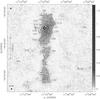 |
Fig. 4 Detailed 870 μm continuum emission maps of Cha I extracted from the map shown in Fig. 2. The flux density greyscale is shown on the right of each panel and labeled in Jy/21.2″-beam. It has been optimized to reveal the faint emission with a better contrast. The angular resolution of the map is shown in the lower left corner of each panel (HPBW = 21.2″). The white plus symbols and ellipses show the positions, sizes (FWHM), and orientations of the Gaussian sources extracted with Gaussclumps or fitted with GAUSS_2D in the filtered map shown in Fig. 5a. The sources are labeled like in the first column of Tables 6, 8, and 9. “C” stands for starless core (or Class 0 protostellar core) and “S” for YSO (Class I or more evolved). In the following, the contour levels are described with the parameter b = 36 mJy/21.2″-beam, i.e. about 3 times the rms noise level. a) Field Cha-North. The contour levels are − b (in dotted blue), b, 2b, 3b, 4b, 5b, 6b, 9b, 12b, 18b, 24b and 30b. The white, thin cross marks the SEST position of Cha-MMS2 (Reipurth et al. 1996). |
 |
Fig. 4 continued. b) Northern part of field Cha-Center. The contour levels are − b (in dotted blue), b, 2b, 3b, 4b, 5b, 6b, 8b, 10b, 12b, 14b, 18b, 22b, 26b, 30b, and 34b. The white, thin cross marks the SEST position of Cha-MMS1 (Reipurth et al. 1996). |
 |
Fig. 4 continued. c) Southern part of field Cha-Center. The contour levels are − b (in dotted blue), b, 2b, 3b, 4b, 5b, 6b, 9b, 15b, 21b, 32b, 48b, and 64b. |
Twelve4 LABOCA sources classified as bona-fide starless cores (C) in Table 2 have a possible SIMBAD association within their FWHM ellipse (Ngcl = 6, 8, 11, 13 14, 15, 24, 26, 29, 39, 59, and 60). They are still classified as starless cores because either they are extended and do not show any evidence for a compact structure at the position of the possibly associated SIMBAD source, or their peak position is significantly offset from it. We consider that the SIMBAD source is either not physically associated with the dense core (chance association, especially in the large dense core in Cha-Center where an IR cluster overlaps with its outskirts) or it is embedded in the dense core but the latter may still form an additional star. However, we cannot exclude that a fraction of these twelve dense cores are remnant of a previous episode of star formation and will never form new stars.
Cha I was observed with the Spitzer instruments IRAC and MIPS in the
framework of the Gould’s Belt legacy program (Allen et al.
2006). The maps are currently being analysed (Jørgensen et al., in prep.) and
were used to search for possible associations with the LABOCA sources. Among the 60 LABOCA
sources classified as bona-fide starless cores (C), 7 have a compact counterpart in
emission in the 24 or 70 μm Spitzer MIPS maps within a
radius of 15″. These Spitzer sources are listed in Table 4. The first one (Nsp = 1)
is associated with source Ngcl = 4 (Cha-MMS1) and was already
reported by Belloche et al. (2006), who argued that
it is a very young Class 0 protostar, or maybe even at the stage of the first hydrostatic
core. At this stage, the mass in the protostellar envelope completely dominates the mass
of the stellar embryo. Therefore it makes sense to compare its properties with those of
starless cores and we keep it in category C. Note that the peak of the
870 μm emission is actually a bit shifted compared to the position
fitted by Gaussclumps and reported in Table 2. The deviation comes from
the asymmetry of the core. By eye, we measure a peak position
(α,δ)J2000 = ( ,
,
 ),
i.e. much closer to the Spitzer position with a relative offset (–0.6″,
–1.1″), which strengthens the association of the Spitzer source with the
870 μm source Ngcl = 4 even further.
),
i.e. much closer to the Spitzer position with a relative offset (–0.6″,
–1.1″), which strengthens the association of the Spitzer source with the
870 μm source Ngcl = 4 even further.
The second and third Spitzer sources (Nsp = 2 and 3) are coincident within 0.3″ with SIMBAD YSOs already listed in Table 2. Their mid-IR slope indicates that they are Class II objects (Jørgensen et al., in prep.). The fourth and fifth Spitzer sources (Nsp = 4 and 5) are also coincident with SIMBAD objects, but only within 3″, which makes the association less secure. Their mid-IR slope indicates that they are Class II and flat-spectrum objects, respectively. The four 870 μm sources Ngcl = 13, 14, 24, and 26 possibly associated with the Spitzer sources Nsp = 2 to 5 are extended. Since they do not show evidence for a compact structure toward the Spitzer source, we still classify them as bona-fide starless cores (C). The last two Spitzer sources (Nsp = 6 and 7) are Class I and II objects, respectively, according to their mid-IR slope, but they do not have any SIMBAD counterpart. They are located ~6″ and ~7″ from the peak of the 870 μm sources Ngcl = 37 and 39, respectively. Since the latter are also extended and do not show evidence for a compact structure, we also still classify them as bona-fide starless cores (C).
In summary, out of 84 sources found with Gaussclumps in the 870 μm map of Cha I, 76 look like real sources. Sixteen of these sources (21%) are associated with a young stellar object (Class I or more evolved) and most likely trace a circumstellar disk and/or a residual circumstellar envelope. The remaining 60 sources (79%) appear to be starless based on Spitzer or contain an embedded Class 0 protostar or first hydrostatic core (one case). The position, sizes, and orientation of these 76 sources, plus the additional sources mentioned in Sect. 5.4 below, are shown in Figs. 4a to g. The labels correspond to the first column of Tables 6, 8, and 9. “C” stands for starless core (or Class 0 protostellar core) and “S” for YSO (Class I or more evolved).
5.4. Additional sources
Since the detection threshold for Gaussclumps was set to 5σ, compact sources with a SIMBAD counterpart and a 870 μm detection between 3.5σ and ~5σ that may be trusted based on the association were missed by Gaussclumps. Therefore, we also looked for 870 μm emission above 3.5σ in the sum map at scale 5 at the position of each source in the SIMBAD database. Clear associations between a SIMBAD source and a compact 870 μm emission were visually selected and all SIMBAD sources associated with extended emission but no clear peak at 870 μm were discarded, in particular those in the prominent dense cores around Cha-MMS1 and Cha-MMS2. As a result, there are five additional compact 870 μm sources with a likely SIMBAD association and a formal peak flux density above 3.5σ. They are listed in Table 5, along with the parameters derived from a Gaussian fit performed with the task GAUSS_2D in GREG5. The fitted peak flux density is below 3.5σ in one case. Given the number of SIMBAD sources in the Cha I field (1045 objects over 1.6 deg2), the probability of chance association within a radius of 5″ is 0.4% only, so we are confident that these five additional SIMBAD associations are real.
6. Analysis
6.1. Starless cores
The properties of the 60 starless (or Class 0) sources are listed in Table 6 and their distribution is shown in Figs. 6 and 8. The column density (Col. 6) and masses (Cols. 8–10) are computed with the fluxes fitted with Gaussclumps or directly measured in the sum map at scale 5, assuming a dust mass opacity κ870 = 0.01 cm2 g-1. As a caveat, we remind that the assumption of a uniform temperature may be inaccurate and bias the measurements of the masses and column densities, as well as the mass concentration (or equivalently the density contrast). Since only one of the 60 sources has an embedded YSO (as traced at 24 μm with Spitzer, see Sect. 5.3), the other 59 have no central heating and their temperature should be rather uniform. However a dust temperature drop toward the center of starless dense cores is possible (see Appendix B.2).
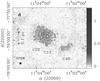 |
Fig. 4 continued. d) Field Cha-South. The contour levels are − b (in dotted blue), b, 2b, and 3b. |
 |
Fig. 4 continued. e) South-eastern part of field Cha-West. The contour levels are − b (in dotted blue), b, 2b, 4b, and 7b. |
6.1.1. Extinction
 |
Fig. 4 continued. f) North-eastern part of field Cha-West. The contour levels are − b (in dotted blue), b, 2b, 3b, and 4b. |
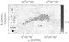 |
Fig. 4 continued. g) North-western part of field Cha-West. The contour levels are − b (in dotted blue), b, and 2b. |
The visual extinctions listed in Table 6 are extracted from the extinction map derived from 2MASS (see Sect. 2.2). Given the lower resolution of this map (HPBW = 3′) compared to the 870 μm map, it provides an estimate of the extinction of the environment in which the 870 μm sources are embedded.
The 870 μm sources are found down to a visual extinction AV ~ 5 mag (as traced with 2MASS at low angular resolution), but not below. A similar result was obtained by Johnstone et al. (2004) in Ophiuchus (threshold at AV = 7 mag), by Enoch et al. (2006) and Kirk et al. (2006) in Perseus (threshold at AV = 5 mag), and by André et al. (2010a) in Aquila (threshold at AV = 5 mag, see Fig. 5 of André et al. 2010b, but see below for the peak of the distribution). In Taurus, Goldsmith et al. (2008) also found a threshold at AV = 6 mag based on the distribution of YSOs, somewhat lower than the earlier findings of Onishi et al. (1998) who proposed a threshold at NH2 = 8 × 1021 cm-2 (AV ~ 9 mag) based on C18O cores and IRAS sources. In both latter cases, however, this threshold is not sharp but rather indicates a significant increase in the probability for star formation to occur.
The extinction toward the only confirmed young protostar in Cha I (Cha-MMS1 or Cha1-C1 in Table 6) is high, at AV = 14 mag. The distribution of extinctions of the environment in which the starless cores are embedded has a median of 9.1 mag and presents a sharp peak at AV ~ 8–9 mag (see Fig. 6e). This is very similar in shape to the distribution of extinctions found for Aquila with Herschel, which peaks at AV ~ 7.5 mag (see Fig. 5 of André et al. 2010b).
Star formation is more likely at high extinction, as discussed above, and in Cha I the
areas of high extinction are small. We can further quantify the relationship between the
extinction and the location of the dense cores using the distribution of extinctions
across the map (Fig. 7a). We calculate the average
surface density of cores  in each extinction bin by dividing the number of starless (+ Class 0) cores in that bin
by the total area of the map (in pc2) in that extinction range. The resulting
average surface density of cores is plotted as a function of gas column density
Σgas (as measured by AV) as a blue histogram in
Fig. 7b.
in each extinction bin by dividing the number of starless (+ Class 0) cores in that bin
by the total area of the map (in pc2) in that extinction range. The resulting
average surface density of cores is plotted as a function of gas column density
Σgas (as measured by AV) as a blue histogram in
Fig. 7b.
If we assume that each core will ultimately form a star, then we could adopt the
extragalactic concept of the Kennicutt-Schmidt law and convert the density of cores to a
star formation rate ΣSF in
M⊙ yr-1 kpc-2. Assuming a mean
lifetime in the detectable prestellar (+ Class 0) stage of 0.5 Myr (see Sect. 7.4) and a mean final stellar mass of
0.5 M⊙ would give a conversion factor from ΣSF
in M⊙ yr-1 kpc-2 to
 in pc-2 equal to 1.
To quantify the relationship between star formation and gas column density in this
local cloud we fit a power law of the form  . One has to be
very careful with the uncertainty budget when dividing two quantities each of which may
lie close to zero, particularly if this applies for the denominator, and here the area
of the cloud becomes small at high extinction. We assume the uncertainties are dominated
by Poisson (
. One has to be
very careful with the uncertainty budget when dividing two quantities each of which may
lie close to zero, particularly if this applies for the denominator, and here the area
of the cloud becomes small at high extinction. We assume the uncertainties are dominated
by Poisson ( )
counting statistics in each extinction bin and use the Bayesian method as laid out in
Hatchell et al. (2005, Appendix A) to calculate
the resulting uncertainties on the ratio. The greyscale in Fig. 7b gives the probability distribution for the true value of the mean
surface density of cores for each AV value, given the
measured counts and assuming Poisson statistics. At high extinction values, where the
number of pixels is close to zero, the mean surface density of cores is very uncertain
and this shows as a broad spread in the greyscale. Using these uncertainties, we perform
a minimisation to calculate the power-law index α and its associated
uncertainties. Fitting over the full range (Av = 0–20) gives
a steep power-law index
)
counting statistics in each extinction bin and use the Bayesian method as laid out in
Hatchell et al. (2005, Appendix A) to calculate
the resulting uncertainties on the ratio. The greyscale in Fig. 7b gives the probability distribution for the true value of the mean
surface density of cores for each AV value, given the
measured counts and assuming Poisson statistics. At high extinction values, where the
number of pixels is close to zero, the mean surface density of cores is very uncertain
and this shows as a broad spread in the greyscale. Using these uncertainties, we perform
a minimisation to calculate the power-law index α and its associated
uncertainties. Fitting over the full range (Av = 0–20) gives
a steep power-law index  (68.3% confidence limits). This is even steeper than the power law found in Perseus
(α = 3.0 ± 0.2, Hatchell et al.
2005). The power-law fit suggests an alternative interpretation to that of an
AV threshold, which is that star formation is simply
unusual at low column densities, and a wide area search is required to find a dense core
which is not embedded in an extended area of raised extinction (Hatchell et al. 2005).
(68.3% confidence limits). This is even steeper than the power law found in Perseus
(α = 3.0 ± 0.2, Hatchell et al.
2005). The power-law fit suggests an alternative interpretation to that of an
AV threshold, which is that star formation is simply
unusual at low column densities, and a wide area search is required to find a dense core
which is not embedded in an extended area of raised extinction (Hatchell et al. 2005).
 |
Fig. 5 a) 870 μm continuum emission sum map of Cha I at scale 5 (see Sect. 5.1). The contour levels are − a (in dashed blue), a, 2a, 4a, 8a, 16a, and 32a, with a = 48 mJy/21.2″-beam, i.e. about 4 times the rms noise level. b) Smoothed map, i.e. residuals, at scale 5. The contour levels are − c (in dashed blue), c, 2c, 4c, and 8c, with c = 13.5 mJy/21.2″-beam, i.e. about 4.5 times the rms noise level in this map. The labels indicate the filaments listed in Table 10. The greyscales of both maps are different. The sum of these two maps is strictly equal to the original map (Fig. 2). |
However, we note that the previous fit tends to underestimate the mean surface density of cores in the range 8–10 mag (see insert of Fig. 7b), where the peak of the distribution in number is located (Fig. 6e). This suggests that the peak at AV ~ 8–9 mag may have a specific physical signification, as proposed by André et al. (2010a) (see Sect. 1).
6.1.2. Sizes
The source sizes along the major and minor axes before and after deconvolution are
listed in Cols. 3 and 4 of Table 6, and their
distribution is shown in Figs. 6a and b,
respectively, along with the distribution of mean size (geometrical mean of major and
minor sizes, i.e.  ).
The average major, minor, and mean sizes are
).
The average major, minor, and mean sizes are  ,
,
 ,
and
,
and  ,
respectively. Only three sources have a major FWHM size larger than
110″, and no source has a minor or mean FWHM size larger than 80″. The
results of the Monte-Carlo simulations in the elliptical case (Appendix A.1 and Table A.1) imply that these sources, although most of them are faint with a peak
flux density lower than 150 mJy/beam, are not significantly affected by the spatial
filtering due to the sky noise removal, with less than 15% loss of peak flux density and
size.
,
respectively. Only three sources have a major FWHM size larger than
110″, and no source has a minor or mean FWHM size larger than 80″. The
results of the Monte-Carlo simulations in the elliptical case (Appendix A.1 and Table A.1) imply that these sources, although most of them are faint with a peak
flux density lower than 150 mJy/beam, are not significantly affected by the spatial
filtering due to the sky noise removal, with less than 15% loss of peak flux density and
size.
The fitting done on the control sample of artificial, circular, Gaussian sources shows
that the accuracy of the sizes derived for sources with a peak flux equal to
~5σ is roughly 20% (see Figs. A.1c and d). With HPBW = 21.2″, the size accuracy of
a weak ~5σ unresolved source is 4.2″. Therefore, faint
sources with a size smaller than ~25.4″ cannot be reliably deconvolved and we
artificially set their size to 25.4″ to perform the deconvolution. As a result the
minimum deconvolved FWHM size that we can measure is ~14″
(2100 AU). The average deconvolved mean FWHM size is
 ,
i.e.
,
i.e.  AU
(see Fig. 6b).
AU
(see Fig. 6b).
Classification of the sources extracted with Gaussclumps from the 870 μm continuum sum map of Cha I at scale 5.
Enoch et al. (2008) measure average deconvolved
mean sizes of 16 500 ± 6000, 10 700 ± 3100, and 7500 ± 3500 AU
(FWHM) for the starless cores extracted with Clumpfind
from their Bolocam maps of Perseus, Serpens, and Ophiuchus, respectively (see
Col. 9 of Table 7). With the MPIfR 19-channel
bolometer array of the IRAM 30 m telescope (HPBW = 15″ after
smoothing), Motte et al. (1998) derive
significantly smaller sizes for the starless cores in Ophiuchus based on a method
similar to the one used here for Cha I (multiresolution decomposition and Gaussian
fitting): they find an average deconvolved mean size of
 AU
when rescaled to the same distance as assumed by Enoch
et al. (2008). Both the differences in angular resolution (31″ versus 15″) and
in the extraction method used (no background subtraction versus multiresolution
analysis) certainly explain the discrepancy of a factor of 3 between both studies. Using
Gaussclumps without background subtraction, Curtis & Richer (2010) derive an average deconvolved mean
size of 3800 ± 200 AU for the starless cores observed in Perseus by Hatchell et al. (2005) with SCUBA, i.e. a factor of
4 times smaller than the Bolocam cores. The angular resolution may therefore be the
dominant factor influencing the derived FWHM sizes. The angular
resolution of LABOCA (21″ after smoothing) being a bit larger than the SCUBA and 30 m
resolutions, we can conclude that the Cha I starless cores have similar physical sizes
than the Perseus cores, are probably larger than the Serpens cores (maybe by a factor of
1.5–2), and are certainly larger than the Ophiuchus cores (by a factor of 2–3).
AU
when rescaled to the same distance as assumed by Enoch
et al. (2008). Both the differences in angular resolution (31″ versus 15″) and
in the extraction method used (no background subtraction versus multiresolution
analysis) certainly explain the discrepancy of a factor of 3 between both studies. Using
Gaussclumps without background subtraction, Curtis & Richer (2010) derive an average deconvolved mean
size of 3800 ± 200 AU for the starless cores observed in Perseus by Hatchell et al. (2005) with SCUBA, i.e. a factor of
4 times smaller than the Bolocam cores. The angular resolution may therefore be the
dominant factor influencing the derived FWHM sizes. The angular
resolution of LABOCA (21″ after smoothing) being a bit larger than the SCUBA and 30 m
resolutions, we can conclude that the Cha I starless cores have similar physical sizes
than the Perseus cores, are probably larger than the Serpens cores (maybe by a factor of
1.5–2), and are certainly larger than the Ophiuchus cores (by a factor of 2–3).
Properties of the Spitzer sources possibly associated with a 870 μm source classified C in Table 2.
Additional compact sources with SIMBAD association with a formal peak flux density above 3.5σ in the 870 μm continuum map of Cha I filtered up to scale 5.
No complete survey of Taurus in dust continuum emission exists. Kauffmann et al. (2008) mapped 10 dense cores with MAMBO at the IRAM
30 m telescope. After smoothing to 20″, they identified 23 starless subcores. The
average deconvolved mean FWHM size of this sample is
 AU
(see Table 7). If this small sample is
representative for the entire population of starless cores in Taurus, then the Cha I
starless cores are significantly smaller (by a factor of 3) than the Taurus ones.
AU
(see Table 7). If this small sample is
representative for the entire population of starless cores in Taurus, then the Cha I
starless cores are significantly smaller (by a factor of 3) than the Taurus ones.
Characteristics of starless (or Class 0) sources extracted with Gaussclumps in the 870 μm continuum map of Cha I filtered up to scale 5.
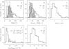 |
Fig. 6 Distribution of physical properties obtained for the 60 starless (or Class 0) sources found with Gaussclumps in the sum map of Cha I at scale 5. The mean, standard deviation, and median of the distribution are given in each panel. The asymmetric standard deviation defines the range containing 68% of the sample. a) FWHM sizes along the major (solid line) and minor (dashed line) axes. The filled histogram shows the distribution of geometrical mean of major and minor sizes. The mean and median values refer to the filled histogram. The dotted line indicates the angular resolution (21.2″). b) Same as a) but for the deconvolved sizes. c) Aspect ratios computed with the deconvolved sizes. The dotted line at 1.4 shows the threshold above which the deviation from 1 (elongation) can be considered as significant. d) Peak H2 column density. The dotted line at 5.25 × 1021 cm-2 is the 5σ sensitivity limit. e) Visual extinction derived from 2MASS. |
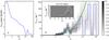 |
Fig. 7 a) Distribution of extinction across the map. The area for AV < 3 regions is limited by the map boundary. b) Mean surface density of starless (+ Class 0) cores as a function of gas column density as measured by AV. For each AV value, the probability distribution for the true value of the mean surface density is displayed in greyscale. The corresponding colorbar on the right is labeled in natural logarithm. The insert is a zoom on the low-extinction range. The best-fit power-law curve to the mean surface density is shown in green/black (see Sect. 6.1.1 for details). |
 |
Fig. 8 Distribution of masses and densities obtained for the 60 starless (or Class 0) sources found with Gaussclumps in the sum map of Cha I at scale 5. The mean, standard deviation, and median of the distribution are given in each panel. The asymmetric standard deviation defines the range containing 68% of the sample. a) Peak mass of the fitted Gaussian. b) Mass within an aperture of diameter 50″. c) Total mass of the fitted Gaussian. The dotted line indicates the estimated completeness limit at 90% for Gaussian sources corresponding to a 6.3σ peak detection limit for the average source size. d) Mass concentration, ratio of the peak mass to the mass within an aperture of diameter 50″. e) Peak density. f) Mean density within an aperture of diameter 50″. g) Density contrast, ratio of peak density to mean density. In panels a) and e), the dotted line indicates the 5σ sensitivity limit. The upper axis of panel d), which can also be used for panel g), shows the power-law exponent p derived assuming that the sources have a density profile proportional to r − p and a uniform dust temperature. Alternately, the upper axis of panel g), which can also be used for panel d), deals with the case where the density is uniform within a diameter Dflat and proportional to r-2 outside, still with the assumption of a uniform temperature. See Sect. 6.1.5 for the limitations of these upper axes. |
Sensitivities of (sub)mm surveys of nearby molecular clouds and average properties of the detected starless cores.
6.1.3. Aspect ratios
The distribution of aspect ratios computed with the deconvolved FWHM
sizes is shown in Fig. 6c. Based on the Monte
Carlo simulations of Appendix A.1, we estimate
that a faint source can reliably be considered as intrinsically elongated when its
aspect ratio is higher than 1.4. 17% of the sources are below this threshold while 83%
can be considered as elongated. The average aspect ratio is
 .
It is similar to the ones measured in Serpens and Taurus, somewhat larger than in
Perseus, and significantly larger than in Ophiuchus (see Col. 10 of Table 7).
.
It is similar to the ones measured in Serpens and Taurus, somewhat larger than in
Perseus, and significantly larger than in Ophiuchus (see Col. 10 of Table 7).
6.1.4. Column densities
The average peak H2 column density of the starless sources in Cha I is
 cm-2
(Fig. 6d). This is 4 times lower than the
average peak column density of the starless cores in Perseus and Serpens, and 3 to 7
times lower than in Ophiuchus (see Col. 11 of Table 7, and Appendix B.6 for details). It
appears to be significantly smaller than in Taurus too (by a factor of 2.6), but since
the Taurus sample is not complete and the source extraction methods differ, this may not
be significant.
cm-2
(Fig. 6d). This is 4 times lower than the
average peak column density of the starless cores in Perseus and Serpens, and 3 to 7
times lower than in Ophiuchus (see Col. 11 of Table 7, and Appendix B.6 for details). It
appears to be significantly smaller than in Taurus too (by a factor of 2.6), but since
the Taurus sample is not complete and the source extraction methods differ, this may not
be significant.
6.1.5. Masses and densities
The distribution of masses and free-particle densities listed in Table 6 are displayed in Fig. 8. The 5σ sensitivity limit used to extract sources with Gaussclumps corresponds to a peak mass of 0.032 M⊙ and a peak density of 2.8 × 105 cm-3, computed for a diameter of 21.2″ (3200 AU). The median of the peak mass distribution is 0.039 M⊙, implying a median peak density of 3.5 × 105 cm-3 (Figs. 8a and e). We give the mass integrated within an aperture of diameter 50″ (7500 AU) in Col. 10 of Table 6. This aperture is well adapted to our sample for three reasons: it corresponds to the average mean, undeconvolved FWHM size (see Sect. 6.1.2 and Fig. 6a), it is not affected by the spatial filtering due to the sky noise removal (see Appendix A.1 and Table A.1), and it is still preserved in the sum map at scale 5 (see Appendix C and Table C.1). The median of the mass integrated within this aperture is 0.10 M⊙, corresponding to a median mean density of 7 × 104 cm-3 (Figs. 8b and f).
The cores in Cha I are about 3–4 times less dense within an aperture of diameter 7500 AU than those in Perseus and Serpens, 6 times less dense than those in Ophiuchus, and 3 times less dense than those in Taurus (see Col. 12 of Table 7, and Appendix B.6.2 for details). However, both studies of Enoch et al. (2008) and Kauffmann et al. (2008) do not filter the extended emission as we do with our multiresolution decomposition to isolate the starless cores from the environment in which they are embedded. This may bias the densities in both studies to somewhat higher values compared to Cha I. In addition, the sensitivities of the different surveys in terms of mass (and mean density) within the aperture of 7500 AU are not the same (see Col. 7 of Table 7). Our survey is more sensitive than those reported by Enoch et al. (2008) by a factor of 2 to 3, but less sensitive than the one of Kauffmann et al. (2008) by a factor of nearly 2. This means that the surveys of Perseus, Serpens, and Ophiuchus may be biased towards higher masses and mean densities and that they may have missed a population of less dense starless cores similar to the one found in Cha I. In the case of Taurus, the bias of the source sample of Kauffmann et al. (2008) prevents any conclusion concerning the possible existence of a population of less dense starless cores.
Figure 8c shows the distribution of total masses computed from the Gaussian fits (Col. 9 of Table 6). The completeness limit at 90% is estimated from a peak flux detection threshold at 6.3σ for the average size of the source sample (FWHM = 49″)6. It corresponds to a total mass of 0.22 M⊙. The median total mass is very close (0.21 M⊙), which implies that only 50% of the detected sources are above the estimated 90% completeness limit. For comparison, the 90% completeness limit of the starless core sample of Enoch et al. (2008) in Perseus is ~0.9 M⊙, i.e. 1.2 M⊙ when rescaled to the same temperature and dust opacity as we use here (12 K and β = 1.85). Our completeness limit is similar to that obtained by Könyves et al. (2010) for their 11 deg2 sensitive continuum survey of the Aquila Rift cloud complex (distance 260 pc) with Herschel: assuming a mass distribution proportional to the radius, they estimated their sample of 541 starless cores to be 75 and 85% complete above masses of 0.2 and 0.3 M⊙, respectively. Their assumed dust opacity law yields κ870 = 0.012 cm2 g-1, i.e. only 20% different from our assumption so the completeness limits can be directly compared.
We estimate the mass concentration of the sources from the ratio of the peak mass to the mass within an aperture of 50″ (Col. 11 of Table 6) which is insensitive to the spatial filtering due to the data reduction (see Table A.1). A similar property is the density contrast measured as the ratio of the peak density to the mean density within this aperture (Col. 14 of Table 6). The statistical rms uncertainties on the peak mass and the mass within 50″ are 0.006 and 0.011 M⊙, respectively, which means a relative uncertainty of up to 20% for the weakest sources. The distributions of both ratios are shown in Figs. 8d and g and their rms uncertainties7 are given in parentheses in Cols. 11 and 14 of Table 6. The two outliers with the largest ratios are also those with the highest relative uncertainty (about 30%). The upper axis of Fig. 8d, which can also be used for Fig. 8g, displays the exponent of the density profile under the assumptions that the sources are spherically symmetric with a power-law density profile, i.e. ρ ∝ r − p, and that the dust temperature is uniform. The median mass concentration and density contrast are 0.39 and 5.1, respectively. This corresponds to p ~ 1.9, suggesting that most sources are significantly centrally-peaked. It is very close to the exponent of the singular isothermal sphere (p = 2). As a caveat, we should mention that the relation used to derive p is valid only for sources with a mass between 21.2″ and 50″ that is measurable and extends up to 50″. In practice, most sources have CM < 50% with a relative uncertainty less than 20% (see Col. 11 of Table 6), meaning that for those sources, the mass between both diameters is measured with a reasonable accuracy. The few sources with CM > 50% (13% of the sample), especially those with CM > 60%, are also those with the highest relative uncertainties (~30% for the latter). The relation to derive p may not be valid for these few sources, or they are simply too weak to give a reliable estimate. As a result, these sources may bias the mean and median values of p to slightly higher values, but since they are not numerous, the bias is certainly small8.
The upper axis of Fig. 8g, which can also be used for Fig. 8d, deals with an alternate case where the sources have a constant density within a diameter Dflat and a density proportional to r-2 outside, still with the assumption of a uniform temperature. Under these assumptions, the measurements are consistent with a flat inner region of diameter 16″ at most (2400 AU) for a few sources, but most sources have Dflat < 10″ (1500 AU), or cannot be described with such a density profile.
6.1.6. Mass versus size
 |
Fig. 9 a) Total mass versus mean FWHM size for the 60
starless (or Class 0) sources found with Gaussclumps in the
sum map of Cha I at scale 5. The angular resolution (21.2″) is
marked by the dotted line. The solid line
(M ∝ FWHM2) is the
5σ peak sensitivity limit for Gaussian sources. The dashed line
shows the 6.3σ peak sensitivity limit which corresponds to a
completeness limit of 90% for Gaussian sources. b) Total mass versus
mean deconvolved FWHM size. Sizes smaller than 25.4″ were set to
25.4″ before deconvolution (see note b of Table 6). The solid line shows the relation
|

The distribution of total masses versus source sizes derived from the Gaussian fits is
shown in Fig. 9a. About 50% of the sources are
located between the 5σ detection limit (full line) and the estimated
90% completeness limit (dashed line), suggesting that we most likely miss a significant
number of sources with a low peak column density. Figure 9b shows a similar diagram for the deconvolved source size. If we assume that
the deconvolved FWHM size is a good estimate of the external
radius of each source, then we can compare this distribution to the
critical Bonnor-Ebert mass that characterizes the limit above which the hydrostatic
equilibrium of an isothermal sphere with thermal support only is gravitationally
unstable. This relation  (Bonnor 1956), with
MBE(R) the total mass, R
the external radius, as the sound speed, and
G the gravitational constant, is drawn for a temperature of 12 K as a
solid line in Fig. 9b. Only three sources (Cha1-C1
to C3) are located above this critical mass limit. If we account for a factor of 2
uncertainty on the mass, then seven additional sources could also fall above this limit
provided the mass is underestimated (Cha1-C4 to C7, C9, C11, and C13, see dash-dotted
line in Fig. 9b). Most sources, however, have a
mass lower than the critical Bonnor-Ebert mass by a factor of 2 to 5. The uncertainty on
the temperature (see Appendix B.2) does not
influence these results much since, even in the unlikely case of the bulk
of the mass being at a temperature of 7 K, the measured masses would move
upwards relative to the critical Bonnor-Ebert mass limit by a factor of 1.9 only,
because the latter is also temperature dependent.
(Bonnor 1956), with
MBE(R) the total mass, R
the external radius, as the sound speed, and
G the gravitational constant, is drawn for a temperature of 12 K as a
solid line in Fig. 9b. Only three sources (Cha1-C1
to C3) are located above this critical mass limit. If we account for a factor of 2
uncertainty on the mass, then seven additional sources could also fall above this limit
provided the mass is underestimated (Cha1-C4 to C7, C9, C11, and C13, see dash-dotted
line in Fig. 9b). Most sources, however, have a
mass lower than the critical Bonnor-Ebert mass by a factor of 2 to 5. The uncertainty on
the temperature (see Appendix B.2) does not
influence these results much since, even in the unlikely case of the bulk
of the mass being at a temperature of 7 K, the measured masses would move
upwards relative to the critical Bonnor-Ebert mass limit by a factor of 1.9 only,
because the latter is also temperature dependent.
Following the analysis of Könyves et al. (2010)
for the Aquila starless cores, we can also estimate the critical Bonnor-Ebert mass with
the equation 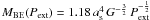 (Bonnor 1956). The external pressure is
estimated with the equation
Pext = 0.88 G (μmHNcl)2,
with μ the mean molecular weight per free particle,
mH the mass of hydrogen, and
Ncl the column density of the local ambient cloud in which
the sources are embedded (McKee & Tan
2003). We use the extinction listed in Table 6 to estimate this background column density with the conversion factors given
in Appendix B.3. The sources with a mass larger
than MBE(Pext) are the same as
for MBE(R), plus Cha1-C4. The agreement
between both estimates of MBE suggests that our estimates of
the external radius and external pressure are consistent. If we account again for a
possible factor of 2 uncertainty on the mass measurement, only three additional sources
would fall above the critical limit based on the pressure (Cha1-C7, C11, and C18). In
summary, four sources are likely above the critical Bonnor-Ebert limit (Cha1-C1 to C4),
and seven additional ones may also be if their mass is underestimated by a factor of 2
(Cha1-C5 to C7, C9, C11, C13, and C18). The implications of this analysis will be
discussed in Sect. 7.
(Bonnor 1956). The external pressure is
estimated with the equation
Pext = 0.88 G (μmHNcl)2,
with μ the mean molecular weight per free particle,
mH the mass of hydrogen, and
Ncl the column density of the local ambient cloud in which
the sources are embedded (McKee & Tan
2003). We use the extinction listed in Table 6 to estimate this background column density with the conversion factors given
in Appendix B.3. The sources with a mass larger
than MBE(Pext) are the same as
for MBE(R), plus Cha1-C4. The agreement
between both estimates of MBE suggests that our estimates of
the external radius and external pressure are consistent. If we account again for a
possible factor of 2 uncertainty on the mass measurement, only three additional sources
would fall above the critical limit based on the pressure (Cha1-C7, C11, and C18). In
summary, four sources are likely above the critical Bonnor-Ebert limit (Cha1-C1 to C4),
and seven additional ones may also be if their mass is underestimated by a factor of 2
(Cha1-C5 to C7, C9, C11, C13, and C18). The implications of this analysis will be
discussed in Sect. 7.
The mass concentration CM is plotted versus source size in Fig. 9c. CM is actually equal to the ratio of the peak flux to the flux integrated within the aperture of diameter 50″. When the sources do not overlap, this ratio is nearly independent of the Gaussian fitting since the second and third stiffness parameters of Gaussclumps were set to 1, i.e. biasing Gaussclumps to keep the fitted peak amplitude close to the observed one and the fitted center position close to the position of the observed peak. The dashed line shows the expected ratio if the (not deconvolved) sources were exactly Gaussian and circular and allows to estimate the departure of the sources from being Gaussian within 50″. Most sources have a mass concentration consistent with the Gaussian expectation, but many of them have a significant uncertainty on CM that prevents a more accurate analysis. The two obvious outliers toward the lower left are sources Cha1-C6 and C8, which have strong neighbors significantly contaminating their flux within 50″ (sources Cha1-S1 and S4, respectively).
 |
Fig. 10 a) Total mass versus visual extinction AV for the 60 starless (or Class 0) sources found with Gaussclumps in the sum map of Cha I at scale 5. The dashed line shows the estimated 90% completeness limit (0.22 M⊙). b) FWHM size versus visual extinction. The angular resolution (21.2″) is marked by the dotted line. |
There is no obvious correlation between the total mass or FWHM size of the sources and the visual extinction of the environment in which they are embedded (see Fig. 10). A similar conclusion was drawn by Sadavoy et al. (2010) for the five nearby molecular clouds Ophiuchus, Taurus, Perseus, Serpens, and Orion based on SCUBA data.
 |
Fig. 11 Mass distribution dN / dMa) and
dN / dlog (M) b) of the 60
starless (or Class 0) sources. The error bars represent the Poisson noise (in
|

6.1.7. Core mass distribution (CMD)
The mass distribution of the 60 starless (or Class 0) sources is shown in Fig. 11, in both forms dN / dM (a) and dN / dlog (M) (b). Its shape in Fig. 11a looks very similar to the shape of the mass distribution found in other star forming regions with a power-law-like behavior at the high-mass end and a flattening toward the low-mass end. In our case, the flattening occurs below the estimated 90% completeness limit (0.22 M⊙) and may not be significant. Above this limit, the distribution is consistent with a power-law. The exponent of the best power-law fit (α = − 2.29 ± 0.30 for dN / dM, αlog = − 1.29 ± 0.30 for dN / dlog (M)) is very close to the value of Salpeter (1955) that characterizes the high-mass end of the stellar initial mass function (α = − 2.35) and steeper than the exponent of the typical mass spectrum of CO clumps (α = − 1.6, see Blitz 1993; Kramer et al. 1998). Such a result was also obtained for the population of starless cores in, e.g., Ophiuchus (α ~ −2.5, Motte et al. 1998), Serpens, Perseus (α = − 2.3 ± 0.4, Enoch et al. 2008), the Pipe nebula (Alves et al. 2007), Taurus (αlog = − 1.2 ± 0.19, Sadavoy et al. 2010), and the Aquila Rift (αlog = − 1.5 ± 0.2, André et al. 2010a; Könyves et al. 2010).
The mass distribution of the Cha I starless sources does not show any significant flattening down to the estimated 90% completeness limit (0.22 M⊙), although the signal-to-noise ratio may not be sufficient to draw a firm conclusion. This seems to contrast with the mass distributions of Ophiuchus and Aquila which flatten below 0.4 and 1.0 M⊙, a factor ~4 and ~3 above their completeness limits, respectively (Motte et al. 1998; Könyves et al. 2010). This flattening translates into a dN / dlog (M) curve with a significant maximum around 0.5–0.6 M⊙ for Aquila while, in Ophiuchus, it keeps increasing with a reduced exponent (αlog ~ −0.5) down to the completeness limit (~0.1 M⊙, Motte et al. 1998). The dN / dlog (M) curve in Cha I reaches a maximum at a mass of 0.2 M⊙ (Fig. 11b), significantly lower than in Aquila. Sadavoy et al. (2010) found a maximum around 0.16 M⊙ for Taurus, which a priori looks similar to our result for Cha I. However, their analysis is based on masses computed within a 850 μm contour of 90 mJy/14″-beam, meaning that they miss a large fraction of the total mass of each core. It is very likely that the mass corresponding to the true maximum is higher than 0.16 M⊙ by a factor of a few, even maybe an order of magnitude. For comparison, the average mass measured by Kauffmann et al. (2008) within an aperture of diameter 8400 AU, which represents only a fraction of the total mass (roughly 50%), is already a factor of 3 higher for their sample of 28 starless “peaks” (see Sect. 6.1.5). The discrepancy with the mass distribution obtained by Onishi et al. (2002) based on H13CO+ observations is even larger, since their distribution dN / dM flattens around 2 M⊙. Therefore, the true maximum of the dN / dlog (M) curve in Taurus is certainly at a mass significantly higher than in Cha I.
6.2. YSO candidates
Characteristics of YSOs extracted with Gaussclumps in the 870 μm continuum map of Cha I filtered up to scale 5.
The sources extracted with Gaussclumps in the sum map at scale 5 and associated with known YSOs found in the SIMBAD database are listed in Table 8. Their possible SIMBAD associations are listed in Table 2. Most of these 16 sources are barely resolved. Their deconvolved sizes are computed from the fitted sizes after multiplying the latter by (1 + 1 / SNR), with SNR the peak signal-to-noise ratio. In this way, the deconvolved sizes are about 1σ upper limits on the true physical sizes of the barely resolved sources. The peak masses, total masses, and masses within an aperture of diameter 50″ are computed with the same assumptions as for the starless sources, except for the dust temperature and mass opacity that we here take as 20 K and 0.03 cm2 g-1, respectively (see Appendix B). The mass concentration CM is higher than 70% for 11 sources (69%), consistent with those sources being nearly point-like and dominating their environment within a diameter of 50″. The remaining 5 sources are contaminated by nearby sources (case of Cha1-S2 and S4) or were qualified as “candidate” (Sc) in Table 2 because they are significantly embedded in a larger-scale dense core and are difficult to extract from their environment (Cha1-S13 to S15).
The same analysis was performed for the 5 additional compact sources found in Sect. 5.4 based on a SIMBAD association. Their deconvolved sizes, peak column density, and masses are given in Table 9. They all have a concentration parameter consistent with their being nearly point-like, but the uncertainties are large because they are faint and close to the detection limit.
In total, 21 compact sources associated with a YSO in the SIMBAD database are detected above the 3.5σ level (42 mJy/21.2″-beam) in the 870 μm continuum map of Cha I. This represents about 10% of the known YSO members of Cha I (237 YSOs, see Luhman 2008). The infrared class of the nearest YSO associated to each compact source is given in Tables 8 and 9. There are 3 Class I, 2 “Flat”, and 16 Class II sources. This represents a 870 μm detection rate of 75%, 20%, and 17% for the respective infrared classes, based on the census of Luhman (2008) (see Table 11). Two of the detected Class II sources are transitional disks, i.e. objects for which the spectral energy distribution indicates central clearings or gaps in the dust distribution (Cha-S5 and S6, see Kim et al. 2009). The missing Class I YSO not listed in Tables 8 and 9 (2M J11092855-7633281 in Luhman 2008) is located about 8″ east of Cha-C12. Given that Cha-C12 is extended and does not show any peak at the position of the YSO, we did not consider the 870 μm emission as being primarily associated with the YSO itself. We can however not exclude that part of this emission comes from the disk and/or the residual envelope of this YSO.
6.3. Large scale structures
The smoothed map at scale 5 clearly shows the two main filamentary structures in fields Cha-Center and Cha-North already mentioned in Sect. 4.1 (see Fig. 5b). It also reveals two fainter filaments that seem to be connected with a T shape in the south-western part of field Cha-Center. Two other faint, elongated, large-scale structures are present in fields Cha-Center and Cha-South, respectively. These filamentary structures were already noticed by Haikala et al. (2005) in their C18O 1–0 map where they appear to be broader, certainly because their map is more sensitive to lower densities than our 870 μm dust emission map. These authors mentioned that the C18O filaments are oriented at roughly right angles to the magnetic field (see their Fig. 8).
The properties of the filamentary structures detected with LABOCA were obtained with Clumpfind. Since we are here interested in the largest structures, only one contour level at 10 mJy/21″-beam (about 3.3σ in the smoothed map) was defined to run Clumpfind. In this way, these filaments were not splitted into sub-structures. Clumpfind extracted 11 structures. Only those with a peak flux density higher than 40 mJy/beam were selected. Their properties are listed in Table 10 and they are labeled in Fig. 5b accordingly. The major and minor sizes given in Table 10 correspond to the full extent of each filament measured by hand using the contour at 10 mJy/beam.
The length of the filaments varies between 6′ and 22′ (0.25 and 1 pc) and their width between 2.3′ and 4.9′ (0.1 and 0.2 pc). Their aspect ratio ranges from 2 to 7. The Monte Carlo simulations performed in Appendix A.1 (see Table A.1) show that weak elliptical sources with a minor FWHM larger than 2.0′, i.e. a full extent along the minor axis larger than ~4.0′, lost more than 15% of their peak flux density and size because of the correlated noise removal of the data reduction. Filaments 1, 3, and the widest filament of the T-shaped structure 4 may therefore be affected by this spatial filtering and their intrinsic widths may be somewhat larger than measured here. On the other hand, the measured width of filaments 2, 5, and of the thinnest filament of structure 4 likely corresponds to their actual minor size. The total mass of these filaments was measured in the full map (Fig. 2) within the contour defined above in the smoothed map at scale 5. They are listed in Col. 16 of Table 10, as well as the corresponding mass per unit length along the major axis in Col. 17.
With a total flux in the smoothed map at scale 5 of 59 Jy, corresponding to a mass of 31 M⊙, these filaments contribute to 52% of the total 870 μm flux measured in Cha I. Their mean H2 column density is relatively low, varying from 2 to 5 × 1021 cm-2, equivalent to a visual extinction AV from 2 to 5 mag. When the mass included in the smaller scales is added (i.e. in the sum map at scale 5), the total mass of these filaments becomes 53 M⊙, i.e. about 88% of the total mass traced with LABOCA in Cha I.
6.4. Comparison with extinction and C18O 1–0 emission
6.4.1. Correlation between continuum emission and AV
 |
Fig. 12 Extinction map of Fig. 1 (red contours) overlaid on the 870 μm continuum emission map of Cha I (black contours). The contour levels of the extinction map increase from 3 to 18 mag by step of 3 mag. The thicker red contour corresponds to AV = 6 mag. The contour levels of the 870 μm map are the same as in Fig. 2. The dotted line delimits the field mapped at 870 μm. The field of view of LABOCA and the angular resolution of the extinction map are shown in the upper right corner. |
The 870 μm dust continuum emission map of Cha I and the extinction map derived from 2MASS are overlaid in Fig. 12. The overall correspondence is relatively good, especially in field Cha-North. In the other fields, the extinction peaks are somewhat shifted compared to the 870 μm peaks, but these shifts ( < 2′) are smaller than the angular resolution of the extinction map and may not be significant. The only exception is close to Cha-MMS1 (C1) in field Cha-Center, where the extinction map peaks about 5′ north-east of the 870 μm peak. This offset still remains when the 870 μm map is smoothed to 3′, showing that it does not result from the different angular resolutions of the original data. An explanation could be that the extinction map does not trace well the H2 column density in this high-extinction region. The average intrinsic colors of the small number of background stars detected in each resolution element of this part of the map may deviate significantly from the assumed average intrinsic colors (Sect. 2.2). Another contributing effect could be the spatial filtering of the 870 μm data. The extinction map (and the C18O 1–0 map, see Sect. 6.4.2) suggests a structure more extended toward the north-east than traced by LABOCA. This missing extended structure could bias the peak position of the 3′-smoothed 870 μm map toward the south-west.
The 4σ H2 column density sensitivity limit of the 870 μm map is 4.2 × 1021 cm-2, which corresponds to AV ~ 4.5 mag. Most of the continuum emission detected at 870 μm is above the contour level AV = 9 mag, and most extended regions with 4.5 < AV < 9 mag traced by the extinction map are not detected at 870 μm. This is due to the spatial filtering related to the sky noise removal (see Appendix A.1) since these low-extinction regions have sizes on the order of 10′–20′, larger than the field of view of LABOCA, especially in fields Cha-Center and Cha-South. On the other hand, there are also a few 870 μm clumps detected between 4.5 and 9 mag that are not seen in the extinction map, most likely because of its poor angular resolution (e.g. Cha1-C13 and C22 in the southern part and Cha1-C20 and C45 in the eastern part). A few YSO candidates are even found below 3 mag (e.g. Cha1-S5, S17, and S18 in field Cha-West, Cha1-S20 and S21 in field Cha-North).
6.4.2. Correlation between C18O 1–0 emission and AV
 |
Fig. 13 a) Integrated intensity map of C18O 1–0 emission detected
with the SEST by Haikala et al. (2005) in
|

The extinction map derived from 2MASS is compared with the C18O 1–0 map obtained by Haikala et al. (2005) with the SEST in Fig. 13a. We smoothed the C18O 1–0 map to an effective angular resolution of 3′ and a pixel size of 1.5′, to match those of the extinction map. The correlation between the two tracers looks very good above AV = 6 mag where the C18O 1–0 integrated intensity is proportional to the visual extinction in good approximation (see Fig. 13b). The high-extinction end (AV > 15 mag) is however not well constrained.
At low extinction (AV < 6 mag), the C18O 1–0 integrated intensity drops steeply with decreasing extinction. This sharp decrease is most likely due to photodissociation. The photodissociation models of Visser et al. (2009) show such a steep C18O column density variation in the range of extinction they investigated (slope ~2 to 7 in a log-log diagram for AV < 5 mag, depending on the density and the UV field). The extension of their model to AV ~ 15 mag (Visser 2010, priv. comm.) shows that for a density nH = 300 cm-3, the turnover occurs at AV ~ 4–5 mag for a UV-field scaling factor of 1–10 and a gas temperature of 15 K, while it occurs at AV ~ 2–3 mag for nH = 1000 cm-3 and at AV ~ 7–8 mag for nH = 100 cm-3. The density of free particles corresponding to the median extinction in Cha I is ~350 cm-3 (see Sect. 4.2), i.e. nH ~ 590 cm-3. This density, which should characterize the density close to the edges of the cloud better than the mean density, should imply a turnover between AV ~ 2–3 and 4–5 mag according to the models of Visser et al. A reason why the turnover in Cha I occurs at a higher level (AV ~ 6 mag10) may be that the low-density medium is inhomogeneous and the UV radiation can penetrate deeper in the cloud than predicted by the homogeneous model of Visser et al.
It follows from the previous paragraphs that the C18O 1–0 emission does not trace well the cloud mass at AV < 6 mag but that it is well correlated with the extinction between AV = 6 and ~15 mag and should thus be a reliable tracer of mass in this range of extinction. We would then expect C18O 1–0 to trace about the same mass as the extinction map above AV = 6 mag (220 M⊙, see Sect. 4.2). Haikala et al. (2005) derived a mass of 230 M⊙ from the C18O 1–0 map shown in Fig. 14a. This map does not contain field Cha-West. This field was covered by Mizuno et al. (1999) and its total C18O 1–0 integrated intensity represents an additional contribution of 15%. The mass traced by C18O 1–0 in Cha I is thus about 260 M⊙. Given the uncertainties on the C18O abundance, the excitation temperature, and the AV-to-mass conversion, this is in very good agreement with the mass derived from the extinction map above AV = 6 mag.
6.4.3. Comparison of continuum emission with C18O 1–0 emission
 |
Fig. 14 a) Integrated intensity map of C18O 1–0 emission detected
with the SEST by Haikala et al. (2005) in
|
The 870 μm dust continuum emission is much less correlated with the C18O 1–0 emission than the 2MASS extinction, as shown in Fig. 14a. We smoothed the 870 μm continuum map to an effective angular resolution of 45″ and a pixel size of 30″ to match the C18O map resolution and pixel size11. The ratio of C18O 1–0 integrated intensity to 870 μm peak flux density is shown in Fig. 14b in color scale. It varies by more than one order of magnitude, being the lowest at the 870 μm peaks. If we assume that the dust temperature and the excitation temperature of C18O 1–0 are the same, the gas-to-dust mass ratio is uniform, and the line is optically thin (see Haikala et al. 2005), then the ratio plotted in Fig. 14b should roughly trace the CO abundance. Its variations point to significant CO depletion toward the center of the 870 μm sources12. Figure 14c displays the relation between the C18O 1–0 integrated intensity and the 870 μm flux density for all pixels above 3σ. Again, this plot shows the poor correlation between both tracers. In addition, a linear fit in log-log space yields a slope of ~0.2, far from what would be expected if C18O 1–0 were tracing the 870 μm continuum emission well (see the red versus blue lines in Fig. 14c).
However, these figures are a priori biased because of the spatial filtering of the 870 μm data that does not affect the C18O 1–0 data. The mass traced by the 870 μm map represents only ~30% of the mass derived from C18O 1–0 (see Sect. 4.2). Since the estimate of the latter does not take into account depletion in regions of high column density, the discrepancy between both tracers must be even worse than a factor of 3. A proper correction would be to filter the C18O 1–0 data in the same way as the 870 μm data are filtered. This is not an easy task and, because of the undersampling of the C18O 1–0 data, may not be fully reliable either. At this stage of the analysis, we cannot exclude that a significant part of the spatial variations seen in Fig. 14b are due to the filtering of the continuum data rather than solely to variations of the C18O abundance.
7. Discussion
7.1. Evolutionary state of Cha-MMS1 and Cha-MMS2
Cha-MMS1 and Cha-MMS2 were the only two dense cores known in Cha I before our LABOCA survey. Reipurth et al. (1996) discovered them at 1.3 mm with the SEST and suggested that both could be Class 0 protostars based on their tentative association with known outflows. In Cha-North, the peak of the 870 μm emission detected with LABOCA (source S3) corresponds to the source Cha-MMS2 detected by Reipurth et al. (1996) within 7″, which is certainly within the errors of the SEST measurements that were performed with a single-channel bolometer. Our source S3 is clearly associated with the T Tauri star WW Cha (coincidence within 1.2″, see Table 2). As a result, Cha-MMS2 is associated with WW Cha and is certainly not a Class 0 protostar (see also Lommen et al. 2009,who came to the same conclusion).
Belloche et al. (2006) discovered a faint Spitzer source at 24 and 70 μm located 5–7″ to the east of Cha-MMS1 (source Nsp = 1 in Table 4). They also reported a Spitzer non-detection at 8 μm (see also Fig. 8 of Luhman 2008), at a 3σ level ~9 and 7 times lower than the peak fluxes of the Taurus Class 0 protostars IRAM 04191+1522 and L1521F, respectively. They did not find any evidence for an outflow associated with Cha-MMS1 based on CO 3–2 observations done with APEX, and derived a deuterium fractionation of 11% for N2H+, a value typical for evolved prestellar cores and young protostars. Based on these two results, they concluded that Cha-MMS1 could be at the stage of the first hydrostatic core, i.e. just before the dissociation of H2 and the second collapse. Our LABOCA observations refine the position of Cha-MMS1. The 870 μm emission peaks at a position 1.3″ away from the Spitzer source, which is well within the positional accuracy of our measurement. This strengthens even further the association of Cha-MMS1 with the faint Spitzer source.
Recently, Dunham et al. (2008) found a very tight correlation between the Spitzer 70 μm flux and the internal luminosity of the low-luminosity YSOs of the c2d legacy project. They define the internal luminosity as the sum of the luminosities of the central protostar and its circumstellar disk, if present. With a 70 μm flux of ~200 mJy (Belloche et al. 2006), this correlation implies that Cha-MMS1 has a very low internal luminosity of ~0.015 L⊙. Luminosities ranging between 10-4 and 0.1 L⊙ have been theoretically predicted at the stage of the first core, depending on the collapse model and the amount of rotation (Saigo & Tomisaka 2006; Omukai 2007). The faint luminosity of Cha-MMS1 looks therefore consistent with the luminosity of a first core. It is about 2 and 3 times fainter than the internal luminosities of the young Class 0 protostars L1521F and IRAM 04191+1522, respectively (Dunham et al. 2008). Since IRAM 04191+1522 drives a prominent bipolar outflow (André et al. 1999) and L1521F may also drive a very compact one (Shinnaga et al. 2009), the absence of evidence for an outflow driven by Cha-MMS1 is an additional argument suggesting that it is in a different stage than these two young protostars, i.e. that it may be at the stage of the first core.
We note that Chen et al. (2010) proposed L1448 IRS2E as a candidate first hydrostatic core based on its low bolometric luminosity (Lbol < 0.1 L⊙, with no Spitzer detection at 70 μm and below) and their detection of a compact outflow. Magnetohydrodynamical simulations do predict that a first core may drive an outflow but they predict that it should be slow (a couple of km s-1 at most, see, e.g., Tomisaka 2002; Machida et al. 2008). The outflow of L1448 IRS2E has velocities about one order of magnitude higher than the predictions of Machida et al. (2008), more consistent with velocities predicted for the second outflow produced once the protostar (second core) is formed. It is therefore somewhat unclear whether L1448 IRS2E can really be at the stage of the first core.
On the other hand, the absence of evidence for an outflow powered by Cha-MMS1 does not contradict these MHD simulations since a compact, slow outflow is a priori not ruled out in this source. We thus confirm the suggestion of Belloche et al. (2006) that Cha-MMS1 is a candidate first hydrostatic core.
7.2. Nature of the LABOCA starless sources
In the past decade, the mass distribution of starless dense cores in many nearby molecular clouds as traced mainly by (sub)mm continuum emission (see references in Sect. 6.1.7) was found to have the same power-law behaviour as the stellar IMF toward the high-mass end, while the mass distribution of lower-density clumps traced with CO has a much flatter shape. This was put forward as a strong argument suggesting that the IMF in these low-mass-star forming clouds is essentially set at the early stage of cloud fragmentation already. The consistency of the high-mass end of the mass distribution of the Cha I starless sources with the stellar IMF suggests that they may be prestellar13 in nature, i.e. form stars in the future.
However, the distribution deviates significantly from the stellar IMF at the low-mass end. This CMD is compared to the stellar IMF of Kroupa (2001) and the IMF of multiple systems of Chabrier (2005) in Fig. 11. Since LABOCA does not probe the scales at which members of a (future) multiple system can be seen individually, only the comparison to the IMF of multiple systems should make sense. While the Cha I mass distribution looks consistent with the IMF of multiple systems above ~0.3 M⊙, it deviates significantly below this threshold, the Cha I starless sources being more numerous at the low-mass end than expected from the IMF. Since the completeness limit of the Cha I survey is ~0.2 M⊙, the discrepancy is a priori even worse at very low mass. Such a deviation has already been noticed in Ophiuchus by André et al. (2007) who concluded that a fraction of the lowest-mass starless sources may not be prestellar and that the link between the CMD and the stellar IMF is less robust at the low-mass end than at the high-mass end (see also André et al. 2009). Our LABOCA survey of Cha I supports this conclusion. Follow-up heterodyne observations with MOPRA and APEX to measure the fraction of gravitationally bound sources are underway and should help better understanding the low-mass end of the mass distribution in Cha I.
Only four sources – among them Cha1-C1, i.e. Cha-MMS1, that is not starless (see Sect. 7.1) – have a mass larger than the critical Bonnor-Ebert value, and seven additional ones may also belong to this group if their mass is underestimated by a factor of 2 (see Sect. 6.1.6). As a result, at most 17% of the starless sources appear to be gravitationally unstable and thus likely prestellar, provided their turbulent and magnetic supports are small compared to their thermal support or will vanish if they are not. This fraction is significantly smaller than in Ophiuchus and Aquila. André et al. (2010a) estimate that more than 60% of the 541 starless sources detected with Herschel in Aquila, with a completeness limit similar to ours (see Sect. 6.1.5), are candidate prestellar cores (with MBE / Mtot < 2). Similarly, about 70% of the starless sources detected by Motte et al. (1998) in Ophiuchus with a completeness limit somewhat better than ours have MBE(R) / Mtot < 2 (see definition of MBE(R) in Sect. 6.1.6)14. In Taurus, more than 50% of the starless cores identified by Kauffmann et al. (2008) are gravitationally unstable, but this sample is biased and inhomogeneous so a direct comparison to Cha I is more uncertain.
The very low fraction of candidate prestellar cores among the starless cores detected in Cha I suggests that we may be witnessing the end of star formation in this cloud or, on the contrary, that these starless cores are in a less advanced stage of evolution compared to those in Aquila, Ophiuchus, and Taurus. The latter suggestion is less likely because we already assessed the gravitational state of the cores assuming that they have no turbulent and magnetic support. A reduction of these support mechanisms via turbulence dissipation or ambipolar diffusion could in principle lead to gravitational instability and eventually gravitational collapse, but only if the cores are above the (purely thermal) critical Bonnor-Ebert mass limit already. A reduction of the thermal support via cooling could in principle also lead to a gravitational instability. In Sect. 6.1.6, we estimated that even if the current temperature of the cores is 7 K instead of 12 K, this would not change the current fraction of unstable cores significantly. If the cores are currently at 12 K even in their center (i.e. the masses we measure are correct) and are still cooling down, then the fraction of unstable cores will not change much either, because the Bonnor-Ebert critical mass will decrease by less than a factor of 2 while most cores are at least a factor of 3 below the current critical mass limit. It is thus unlikely that most starless cores that appear to be currently stable will become unstable in the future, unless they experience a strong external perturbation.
7.3. Star formation efficiency
7.3.1. Local star formation efficiency
Apart from the deviation at low mass, the mass scale of the Cha I CMD agrees quite well with that of the IMF of multiple systems in Fig. 11. Taken at face value, this would suggest that the star formation efficiency at the core level in Cha I will be as high as ~100% for all prestellar sources that populate the high mass end above ~0.3 M⊙. For comparison, André et al. (2010a) found an efficiency ϵcore = M ⋆ / Mcore ~ 20–40% in Aquila and Alves et al. (2007) obtained ϵcore = 30 ± 10% for the Pipe nebula. Enoch et al. (2008) could only set a lower limit of 25% for their combined sample of Perseus, Serpens, and Ophiuchus sources, because of their poor completeness limit (0.8 M⊙).
Luhman (2007) computes the specific IMF of the stellar population of Cha I and find a peak at 0.1–0.15 M⊙. If we take this turnover mass as reference, then the (apparent) turnover of the Cha I CMD at the completeness limit still suggests a local star formation efficiency ϵcore > 50–70%. Such a very high efficiency for Cha I sounds a priori unlikely. One explanation could be that the contamination by gravitationally unbound, starless sources (see Sect. 7.2) may extend further to higher masses and mask the maximum of the true prestellar CMD. Indeed, Könyves et al. (2010) found that the peak of the Aquila CMD shifted from 0.6 to 0.9 M⊙ when they removed from their sample the sources that they estimated not to be prestellar (~35%). On the other hand, the majority of the Pipe nebula sources appear to be gravitationally unbound (Lada et al. 2008) and their CMD still closely resembles the IMF in shape (Alves et al. 2007). Therefore it is unclear by how much the Cha I CMD could be affected by contamination from unbound, starless sources. The on-going follow-up heterodyne observations should help answer this question.
7.3.2. Global star formation efficiency
At the scale of the cloud, Luhman (2007)
estimate a current star formation efficiency, defined as
 ,
of about 10%, based on the cloud mass derived from CO
(~1000 M⊙, see Sect. 4.2) and the mass ~100 M⊙ of
the 215 young stars and brown dwarfs known to belong to Cha I at that time. This star
formation efficiency is a factor of 1.5 to 3 larger than the SFEs of the five nearby
molecular clouds targeted by the c2d Spitzer legacy project (between
3.0 and 6.3%, see Table 4 of Evans et al. 2009).
It is even more than one order of magnitude higher than the SFE of the Taurus molecular
cloud (0.6%15, see Goldsmith et al. 2008). Assuming a constant rate of star formation, Evans et al. (2009) suggest that the c2d clouds could
reach a final SFE of 15 to 30% given the estimated typical lifetime of a molecular
cloud. The SFE of Cha I is close to this limit, this being even more true if the rate of
star formation in the c2d clouds decreases with time like in Cha I (see Sect. 7.4), which would reduce the expected final SFE. We
note that Bonnell et al. (2011) find an overall
efficiency of star formation of ~15% in their numerical simulation of a
turbulent, molecular cloud that undergoes star formation. It is thus very likely that
Cha I is much closer to the end of the star formation process than the other clouds
mentioned above.
,
of about 10%, based on the cloud mass derived from CO
(~1000 M⊙, see Sect. 4.2) and the mass ~100 M⊙ of
the 215 young stars and brown dwarfs known to belong to Cha I at that time. This star
formation efficiency is a factor of 1.5 to 3 larger than the SFEs of the five nearby
molecular clouds targeted by the c2d Spitzer legacy project (between
3.0 and 6.3%, see Table 4 of Evans et al. 2009).
It is even more than one order of magnitude higher than the SFE of the Taurus molecular
cloud (0.6%15, see Goldsmith et al. 2008). Assuming a constant rate of star formation, Evans et al. (2009) suggest that the c2d clouds could
reach a final SFE of 15 to 30% given the estimated typical lifetime of a molecular
cloud. The SFE of Cha I is close to this limit, this being even more true if the rate of
star formation in the c2d clouds decreases with time like in Cha I (see Sect. 7.4), which would reduce the expected final SFE. We
note that Bonnell et al. (2011) find an overall
efficiency of star formation of ~15% in their numerical simulation of a
turbulent, molecular cloud that undergoes star formation. It is thus very likely that
Cha I is much closer to the end of the star formation process than the other clouds
mentioned above.
7.4. Lifetimes
The median age of the YSO population of Cha I is ~2 Myr (Luhman 2008)16. With the census of starless cores and YSOs presented in Table 11, we can statistically estimate the lifetimes of each category if we assume that all prestellar cores evolve into Class 0/Class I protostars and then into Class II/Class III YSOs, and that star formation has proceeded at a constant rate over time. Five to 15 YSOs out of 204 are protostars, implying a typical lifetime of 0.5–1.5 × 10⁵ yr for the protostars in Cha I. Only one object is a Class 0 protostar (or first core), hence a very short lifetime of 104 yr for the Class 0 phase. Given that a fraction of the starless cores may not be prestellar in nature (see Sect. 7.2), we can only derive an upper limit of 6 × 10⁵ yr to the duration of the prestellar phase in Cha I.
Census of starless cores and YSOs in Cha I.
The median peak density of the Cha I starless cores is 3.5 × 105 cm-3 and their median mean density within 50″ is 7 × 104 cm-3 (Figs. 8e and f). This median mean density corresponds to a prestellar lifetime of ~4 × 10⁵ yr according to the empirical relation of Ward-Thompson et al. (2007). If the fraction of non-prestellar sources among the Cha I starless sources is on the order of 30% or less, then the agreement between this prestellar lifetime and the lifetime derived from the statistical counts in the previous paragraph suggests that the assumption of a star formation rate constant over time until now is valid in Cha I. It is also consistent with the prestellar lifetime of 4.5 ± 0.8 × 10⁵ yr estimated by Enoch et al. (2008) for their combined sample of Perseus, Serpens, and Ophiuchus (see also Jørgensen et al. 2007,for Perseus alone). The very short lifetime of 104 yr derived here for the Class 0 phase is similar to the one found in Ophiuchus (1–3 × 10⁴ yr, see André et al. 2000), but about one order of magnitude shorter than in Perseus (e.g. Hatchell et al. 2007).
On the other hand, if, e.g., 90% of the Cha I starless sources turn out not to be prestellar in nature, then the unrealistically low statistical lifetime that would be inferred for the prestellar sources (6 × 10⁴ yr) would rather point to a decrease of the star formation rate with time and confirm the trend pointed out by Luhman (2007). This could also explain why so few Class 0 sources (only one) are found in Cha I, if the Class 0 lifetime derived in Perseus rather than in Ophiuchus applies to Cha I. In any case, an increase of the star formation rate until the present time (Palla & Stahler 2000, see Sect. 1) is ruled out for Cha I.
7.5. Filaments
The Herschel satellite has recently revealed an impressive network of parsec-scale filamentary structures in the nearby molecular clouds Aquila and Polaris (e.g. André et al. 2010a; Men’shchikov et al. 2010). The few filaments detected in Cha I with LABOCA (see Sect. 6.3) and in C18O 1–0 (Haikala et al. 2005) are strong evidence for the existence of such a network in this cloud, of which we only see the tip. These filaments have a deconvolved width of 0.16 ± 0.05 pc on average (33 000 AU), measured at a level of 10 mJy/21.2″-beam. This width may be somewhat underestimated because of the spatial filtering due to the correlated noise removal (see Sect. 6.3). It is similar to the typical width of the Perseus filaments as measured by Hatchell et al. (2005) with SCUBA (FWHM ~ 1′, i.e. 15 000 AU at 250 pc). However, the Cha I filaments are less massive, with a mass per unit length ranging between 8 and 33 M⊙ pc-1 (see Table 10) while it ranges between 47 and 115 M⊙ pc-1 for the Perseus filaments (Hatchell et al. 2005).
The mass per unit length of filaments is an essential parameter to evaluate their
stability. In Aquila, most ( > 60%) candidate prestellar cores
were found in (thermally) supercritical filaments defined by
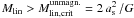 (see André et al. 2010a, and references therein). Only one filament in Cha I
(Nfil = 1) has a mass per unit length larger than the
critical value (19 M⊙ pc-1 at 12 K). It contains
the single Class 0 protostar (Cha1-C1) and two of the three candidate prestellar cores
(Cha1-C2 and C3), while only one of the four other (subcritical) filaments contains a
candidate prestellar core (Cha1-C4 in filament 5). Even if these numbers are much too
small to derive any robust conclusion, they seem to be consistent with the results
obtained by André et al. (2010a) for Aquila.
(see André et al. 2010a, and references therein). Only one filament in Cha I
(Nfil = 1) has a mass per unit length larger than the
critical value (19 M⊙ pc-1 at 12 K). It contains
the single Class 0 protostar (Cha1-C1) and two of the three candidate prestellar cores
(Cha1-C2 and C3), while only one of the four other (subcritical) filaments contains a
candidate prestellar core (Cha1-C4 in filament 5). Even if these numbers are much too
small to derive any robust conclusion, they seem to be consistent with the results
obtained by André et al. (2010a) for Aquila.
However, the total velocity dispersion as probed by C18O 1–0in Cha I is
significantly larger than the purely thermal dispersion. The C18O 1–0 linewidth
(FWHM) is typically on the order of 0.5–0.8 km s-1 (see
Table 1 of Haikala et al. 2005), yielding a
non-thermal velocity dispersion
σNT = 0.20–0.38 km s-1 and an effective sound
speed aeff = 0.29–0.43 km s-1 at 12 K. We can
compute the mean free-particle density nmean of the filaments
with the equation  , with
Nmean and amin given in
Table 10 and
μH2 and μ defined in
Appendix B.5. These mean densities are in the
range 3.7–10 × 103 cm-3. Since the critical density of the
C18O 1–0 line at 10 K is about 3 × 103 cm-3, this
transition traces the bulk of the filaments very well and its linewidth should reliably
trace their total velocity dispersion, although some contamination from the ambient cloud
cannot be completely excluded. If we assume that C18O 1–0 traces only the
filaments, then the critical mass per unit length becomes the virial mass per unit length
, with
Nmean and amin given in
Table 10 and
μH2 and μ defined in
Appendix B.5. These mean densities are in the
range 3.7–10 × 103 cm-3. Since the critical density of the
C18O 1–0 line at 10 K is about 3 × 103 cm-3, this
transition traces the bulk of the filaments very well and its linewidth should reliably
trace their total velocity dispersion, although some contamination from the ambient cloud
cannot be completely excluded. If we assume that C18O 1–0 traces only the
filaments, then the critical mass per unit length becomes the virial mass per unit length
 (Fiege & Pudritz 2000) and ranges from 39 to
86 M⊙ pc-1. The Cha I filaments have a mass per
unit length lower than this critical value by a factor of 2 at least (the velocity
dispersion is the highest in filament Nfil = 1). Unless they
are compressed by a significant toroidal magnetic field (Fiege & Pudritz 2000) or the C18O 1–0 linewidth overestimates
their total velocity dispersion, they do not seem to be supercritical and will most likely
neither collapse nor fragment in the future. This would be consistent with our conclusion
that the process of star formation is nearly over in Cha I.
(Fiege & Pudritz 2000) and ranges from 39 to
86 M⊙ pc-1. The Cha I filaments have a mass per
unit length lower than this critical value by a factor of 2 at least (the velocity
dispersion is the highest in filament Nfil = 1). Unless they
are compressed by a significant toroidal magnetic field (Fiege & Pudritz 2000) or the C18O 1–0 linewidth overestimates
their total velocity dispersion, they do not seem to be supercritical and will most likely
neither collapse nor fragment in the future. This would be consistent with our conclusion
that the process of star formation is nearly over in Cha I.
7.6. The end of star formation in Cha I?
Mass, area, and average surface density of a sample of nearby molecular clouds, measured over the regions with AV > 3 mag, 3 < AV < 6 mag, and AV > 6 mag.
The low fraction of candidate prestellar cores among the population of starless cores detected with LABOCA, the small number of Class 0 protostars, the high global star formation efficiency, the decrease of the star formation rate with time, and the low mass per unit length of the detected filaments all suggest that we may be witnessing the end of the star formation process in Cha I. While the conclusion of Luhman (2007) that the star formation rate in Cha I has declined for several Myr already questions the scenario of Palla & Stahler (2000) in which star formation is a threshold phenomenon and accelerates as a result of cloud contraction (see Sect. 1), our findings raise new questions about the end of star formation. Palla & Stahler (2000) argue that the truncation period, i.e. the period over which the star formation rate drops, must be very brief (1 Myr at most) and that the falloff should be related to the dispersal of the parent cloud gas. In low-mass star forming regions, they consider that this dispersal can only result from the impact of molecular outflows. Even if the total current mass efflux due to molecular outflows in the particular case of Taurus is three orders of magnitude lower than the one needed to disperse the cloud in such a short time, they argue that the (potentially) accelerating nature of star formation should significantly increase the mass efflux in the future and that, if star formation is really a threshold phenomenon, its falloff can occur before the actual cloud dispersal.
To look for signs of cloud dispersal in Cha I, we compare its mass, area, and surface density to those of a sample of nearby molecular clouds in Table 12. We list the surface densities for the low- (3 < AV < 6 mag) and high-extinction (AV > 6 mag) regions in Cols. 8 and 11, respectively. The limit AV = 6 mag approximately corresponds to the extinction threshold for star formation mentioned in Sects. 1 and 6.1.1. If all clouds have similar depths, then the surface density scales with the average density and could be a good indication for cloud dispersal. On the one hand, Cha I has a surface density above AV = 6 mag very similar to the ones of the other clouds, suggesting that the average density of its high-extinction region is the same as in the other clouds, provided its depth is similar to the ones of these clouds. Only Serpens has a significantly lower surface density compared to the rest of the sample. On the other hand, the surface density of Cha I (and Serpens to a lesser extent too) for 3 < AV < 6 mag is significantly higher than in the other clouds. As a result, it stands out, along with Serpens, with a surface-density ratio between the regions with AV > 6 mag and 3 < AV < 6 mag somewhat lower than in the other clouds. Since this ratio does not depend on the depth of the cloud, it could be a more reliable tracer of cloud dispersal and could indicate that Cha I and Serpens are in the process of being dispersed. However, these two clouds do not seem to differ significantly from other nearby star-forming clouds in terms of probability density functions of column density (Kainulainen et al. 2009). Therefore the signs for cloud dispersal in Cha I based on the extinction map are very tenuous. Further clues to explain why Cha I could be at the end of the star formation process should be searched for. Finally, we note that we cannot exclude that the star formation activity in Cha I could be revived in the future if the cloud would undergo a significant external compression
8. Conclusions
We performed a deep, unbiased, 870 μm dust continuum survey for starless and protostellar cores in Chamaeleon I with the bolometer array LABOCA at APEX. The resulting 1.6 deg2 map was compared with maps of dust extinction and C18O 1–0 emission. It was decomposed into multiple scales to disentangle the emission of compact or moderately extended sources from large-scale structures. The analysis was performed by carefully taking into account the spatial filtering properties of the data reduction process. Our main results and conclusions are the following:
-
1.
The standard reduction process of LABOCA data with BoAfilters the emission more extended than ~2.5–4′ (FWHM), depending on itsflux density. Elongated sources are better recovered than circularones along their major axis, up to 6–9′. The iterative schemerequires about 21 iterations to converge.
-
2.
The mass detected with LABOCA (61 M⊙) represents only 6–8%of the cloud mass traced by the dust extinction and CO, and about 30% of the mass traced by C18O. Most (88%) of this 870 μm mass is located in five filaments with typical length and width of 0.6 and 0.16 pc, respectively.
-
3.
The C18O 1–0 emission is a reliable tracer of mass in the visual extinction range 6 to 15 mag. C18O appears to be photodissociated below 6 mag.
-
4.
81 sources were extracted from the 870 μm map, 59 of which are starless based on the absence of Spitzer association, one is a candidate first hydrostatic core (Cha-MMS1), and 21 are associated with more evolved young stellar objects already known in the SIMBAD database.
-
5.
Like in other nearby molecular clouds, the starless cores in Cha I are only found above an extinction threshold AV = 5 mag and their distribution of extinction peaks at AV ~ 8 mag (7 mag with RV = 5.5). Alternatively there may be no strict threshold but just a very low probability of finding a core at low extinction.
-
6.
The 90% completeness limit of our 870 μm survey is 0.22 M⊙ for starless cores. Only 50% of the detected starless cores are above this limit, suggesting that we may miss a significant fraction of the existing starless cores.
-
7.
The starless cores in Cha I are less dense than those in Perseus, Serpens, Ophiuchus, and Taurus by a factor of a few on average. This may result from the better sensitivity of the Cha I survey and/or the multi-scale analysis of the Cha I data.
-
8.
The CO abundance seems to decrease toward the peak of the embedded starless cores, as expected for bona-fide prestellar cores, but the spatial filtering of the 870 μm data prevents a firm conclusion.
-
9.
On the one hand, the high-mass end of the core mass distribution in Cha I is consistent with the stellar initial mass function, suggesting that a fraction of the starless cores may be prestellar. On the other hand, the low-mass end is overpopulated, and at most 17% of the starless cores have a mass higher than the critical Bonnor-Ebert mass. Both results suggest that a large fraction of the starless cores may not be prestellar.
-
10.
The local star formation efficiency at the core level in Cha I ( > 50%) seems to be larger than in other molecular clouds, but this conclusion is uncertain due to possible contamination by unbound, starless sources.
-
11.
The global star formation efficiency at the scale of the cloud is 10%. It is significantly larger than in other clouds and suggests that Cha I is much closer to the end of the star formation process.
-
12.
The star formation rate in Cha I can have been constant over time only if > 70% of the detected starless cores turn out to be prestellar. This is very unlikely, which suggests that the star formation rate has decreased over time, as also indicated by the very small number of Class 0 protostars. An increase of the star formation rate to the present time in Cha I is ruled out.
-
13.
Apart from maybe one, the filaments in which most starless cores are embedded do not seem to be supercritical and will most likely neither collapse nor fragment in the future.
The low fraction of candidate prestellar cores among the population of starless cores detected with LABOCA, the small number of Class 0 protostars, the high global star formation efficiency, the decrease of the star formation rate with time, and the low mass per unit length of the detected filaments all suggest that we may be witnessing the end of the star formation process in Cha I. We only find a tenuous evidence for cloud dispersal based on the distribution of extinction. Further clues to explain why Cha I could be at the end of the star formation process should be searched for.
Online material
Appendix A: LABOCA data reduction: spatial filtering and convergence
A.1. Spatial filtering due to the correlated noise removal
 |
Fig. A.1 Statistical properties of 60 artificial, circular, Gaussian sources inserted into the raw time signals before data reduction a) to e) or directly inserted into the final unsmoothed continuum emission map of Cha I f) to j). a) and f): ratio of output to input peak flux density as a function of input peak flux density. b) and g): ratio of output to input peak flux density as a function of input size (FWHM). c) and h): ratio of output major size to input size as a function of input size. d) and i): ratio of output minor size to input size as a function of input size. e) and j): ratio of output to input total flux as a function of input size. The size of the black symbols scales with the input size of the sources. In addition, crosses and plus symbols are for input peak flux densities below and above 150 mJy/19.2″-beam, respectively. The red circles in panels b) to e) and g) to j) show a fit to the data points using the arbitrary 3-parameter function y = log (α / (1 + (x / β)γ)). |
Since LABOCA is a total-power instrument used without wobbler, the standard data reduction relies on the correlated signal of all pixels and of smaller groups of pixels to estimate and remove the atmospheric and instrumental noise. This method acts as a high-pass filter and makes the detection of very extended structures extremely difficult. The strongest limiting factor is the size of the groups of pixels connected to the same read-out cable (about 1.5′ by 5′, see Schuller et al. 2009). To analyse the dust continuum emission map in detail, it is therefore essential to understand the properties of this spatial filtering.
We performed several Monte Carlo simulations to characterize the filtering. First, we inserted artificial, circular, Gaussian sources in the raw time signals with the BoA method addSource after calibration. The sources were inserted at random positions in signal-free regions of the map shown in Fig. 2. The peak flux densities and FWHM sizes of the sources were randomly assigned in the range 50 to 500 mJy/beam and 19.2″ to 8′, respectively. The only constraint was that the artificial sources should not overlap and should not be too close to the map edges either. The modified raw data were then reduced following exactly the same procedure as described in Sect. 3.1, except that the final map was not smoothed and kept its original angular resolution of 19.2″ (HPBW). Each artificial source was fitted with an elliptical Gaussian using the task GAUSS_2D in GREG to measure its output peak flux density and sizes after data reduction. We also measured the total output flux on a circular aperture of radius equal to FWHM.
The whole procedure was repeated twice, with two independent samples of 30 artificial sources. Figures A.1a–e present the results. As a control check, we show in Figs. A.1f–j the results of the fits performed on the artificial sources directly inserted in the final unsmoothed continuum emission map of Cha I. The effects of the spatial filtering due to the data reduction are obvious when comparing Figs. A.1b–e to Figs. A.1g–j. The noise produces a small dispersion in the output source properties, especially for weak sources (crosses) but apart from that, all curves are basically flat in the control sample (Figs. A.1f–j). On the contrary, after data reduction, the peak flux densities of the sources are reduced by ~15% to ~70% for input sizes varying from ~240″ to ~440″. Similarly, the sizes of the sources are reduced by ~15% to ~50% for input sizes from ~200″ to ~440″. The total fluxes suffer the most from the spatial filtering: they are reduced by ~15% to ~90% for input sizes from ~120″ to ~440″. A careful inspection of Figs. A.1g–j shows that the sources with a peak flux density weaker than ~150 mJy/beam (crosses) are systematically below the stronger sources (plus symbols) for source sizes larger than ~100″. This is because the insertion of the stronger sources in the astronomical source model used for iterations 1 to 20 helps to recover more astronomical signal when their outer parts start to reach the thresholds mentioned in Sect. 3.1. The spatial filtering is therefore less severe for strong sources than for faint sources. These results are summarized in Table A.1.
A further Monte Carlo test was performed with elliptical Gaussian sources with a fixed aspect ratio of 2.5. The procedure to generate these artificial sources was the same, with the orientation of the sources also assigned randomly. The peak flux densities ranged between 85 and 500 mJy/beam and the size along the minor axis (FWHM) between 19.2″ and 3.7′. Three sets of sources were analysed, providing a sample of 68 sources in total. The results are very similar to the circular case, but with characteristic scales of the filtering along the minor axis of the elliptical sources 20–25% smaller (see Table A.1). In return, the corresponding characteristic scales of the filtering along the major axis are a factor of 2 larger than in the circular case. The peak flux densities are reduced by ~15% to ~20% for input sizes along the minor axis varying from ~180″ to ~220″ (i.e. sizes from ~450″ to ~550″ along the major axis). The aspect ratio is well preserved within ~10% after the last iteration, but the sizes of the sources are reduced by ~15% to ~25% for input sizes along the minor axis from ~160″ to ~220″ (i.e. from ~400″ to ~550″ along the major axis). Here again, sources with a peak flux density higher than ~150 mJy/beam are better recovered than weaker sources that cannot or can only partly be incorporated into the astronomical source model used at iterations 1 to 20.
These two Monte Carlo tests clearly show that the reduction of LABOCA data based on correlations between pixels to reduce the atmospheric and instrumental noise can have a strong impact on the structure of the detected astronomical sources. Depending on their shape and strength, structures with (major) sizes larger than ~140″–280″ if circular or ~300″–550″ if elliptical with an aspect ratio of 2.5 are significantly filtered out (>15% losses of peak flux density and size). Elongated structures are better recovered than circular ones. We note that the reduction performed for data obtained at the Caltech Submillimeter Observatory (CSO) with the bolometer camera Bolocam suffers from the same problem, with a similar characteristic scale above which losses due to spatial filtering start to be significant (~120″ for circular sources, see Enoch et al. 2006).
Several attemps to attenuate the correlated noise removal by using the outer pixels only, or to suppress the correlated noise removal and replace it subscan-wise with a simple first-order baseline removal in the time signals of the OTF scans, were not successful. These alternative reduction schemes produced somewhat more extended emission in places where we expected some, but at the same time, there were much more atmospheric and instrumental noise residuals distributed within the map that also mimicked extended structures where we did not expect any, by comparison to the extinction and C18O 1–0 maps for instance. Attempts to reduce the data without flattening the power spectrum at low frequency or with a lower cutoff frequency did not bring any significant improvement either.
A.2. Convergence of the iterative data reduction
The iterative process of data reduction described in Sect. 3.1 allows to recover additional astronomical flux after each iteration. In this section, we study the convergence of this method. The evolution of the total 870 μm flux recovered in Cha I as a function of iteration is shown in Fig. A.2a. The relative flux variation is only 0.7% at iteration 20, which suggests that the data reduction process indeed converged.
Filtering of artificial Gaussian sources due to the correlated noise removal depending on the input size along the minor (major) axis (FWHM).
 |
Fig. A.2 a) Convergence of the total 870 μm flux recovered in Cha I by the iterative process of data reduction. b) Relative flux variation between iterations i and i − 1 as a function of iteration number i. |
 |
Fig. A.3 Convergence of the iterative data reduction for artificial, circular, Gaussian sources with a peak flux density larger than 150 mJy beam-1. The first and second columns show the ratio of the output to the input peak flux densities, and its relative variations, respectively. The third and fourth columns show the same for the total flux. The different rows show sources of different widths, as specified in each panel of the first column. The size of the symbols increases with the input peak flux density. |
This experiment shows that a significant number of iterations (about 20) are necessary to recover as much extended emission as possible. Enoch et al. (2006) have a similar conclusion with Bolocam for circular sources with FWHM < 120″ (convergence at iteration 5, see their Fig. 4), but they do not mention or show how many iterations they need to reach convergence17 for much larger sources.
Appendix B: Assumptions
In this Appendix, we explain the various assumptions that are used to analyse and interpret the Cha I data. We also explain how the column densities and average densities obtained in the past for other molecular clouds are rescaled in the present study to compare with Cha I (Table 7).
B.1. Distance
Whittet et al. (1997) analysed the distribution of extinctions of field stars with distance along the line of sight of Cha I and derived a distance of 150 ± 15 pc for this cloud. They also deduced a photometric distance for the B-type star HD 97300 of 152 ± 18 pc. They combined these results with the parallaxes of this and another star (HD 97048) measured with the Hipparcos satellite with a larger uncertainty (190 ± 40 and 180 ± 20 pc, respectively) and adopted a “final” distance of 160 ± 15 pc.
Knude & Høg (1998) used the interstellar reddening from the Hipparcos and Tycho catalogues to derive the distance to Cha I. They found a distance of 150 pc as revealed by a sharp increase in their plot of E(B − V) color excess versus distance.
However, Knude (2010) recently derived a further distance of 196 ± 13 pc for Cha I from a fit to an extinction vs. distance diagram. The extinction was obtained from a (H–K) vs. (J–H) diagram from 2MASS and the distances were estimated from a (J–H)0 vs. MJ relation based on Hipparcos. Rather than considering the distance at which the first stars show a steep increase in extinction as the distance of the cloud, they fitted a predefined function to a subsample of the data. It is unclear to us whether this fitting procedure does give a more reliable distance estimate because the selection of the subsample defining the extinction jump for the fit may introduce a bias. Therefore, as long as this further distance has not been confirmed by another method, we keep the older estimate (150 pc) as the distance of Cha I. If the further distance turns out to be correct, then all physical sizes and masses derived in this article are underestimated by a factor 1.3 and 1.7, respectively, and the mean densities are overestimated by a factor 1.3. The column densities are not affected.
B.2. Temperature
Tóth et al. (2000) derived a dust temperature of 12 ± 1 K for the “very cold cores” they identified in Cha I on somewhat large scales (HPBW ~ 2′) from their analysis of the ISOPHOT Serendipity Survey (see cores 1 to 6 in their Table 2). The dust temperature is most likely not uniform and this value rather represents a mean temperature. The dust temperature is expected to decrease toward the center of starless dense cores that do not contain any central heating, even down to ~5.5–7 K as measured for the gas in the prestellar cores L1544 and L183 by Crapsi et al. (2007) and Pagani et al. (2007), respectively. The modeled dust temperature profiles of the prestellar cores L1512, L1689B, and L1544 derived by Evans et al. (2001) indeed vary from 12–13 K in the outer parts to 7–8 K at the core center. Similarly, Nutter et al. (2008) measured a dust temperature varying from 12 K in the outer parts to 8 K in the inner parts of a filament in the Taurus molecular cloud 1 (TMC1). Thanks to its good angular resolution and its good sampling of the spectral energy distribution of these cores, such temperature variations will be routinely measured in the far-infrared with the Herschel satellite, which will help refining the mass and column density estimates (see, e.g., André & Saraceno 2005). For simplicity, we assume here a uniform dust temperature of 12 K.
If the temperature inside the dense cores drops to, e.g., 7 K, their masses and column densities computed in this article could be underestimated by up to a factor of 3, depending on the exact shape of the temperature profile. However, the total mass of a core being dominated by its outer parts, it should not be that much underestimated.
B.3. Conversion of visual extinction to H2 column density
The standard factor to convert a visual extinction AV to an H2 column density is 9.4 × 1020 cm-2 mag-1. It is based on the ratio NH / E(B − V) = 5.8 × 10²¹ atoms cm-2 mag-1 measured by Bohlin et al. (1978) with data from the Copernicus satellite, and a ratio of total-to-selective extinction RV = AV / E(B − V) = 3.1 corresponding to the standard extinction law that is representative of dust in diffuse regions in the local Galaxy (see, e.g., Draine 2003,and references therein).
Several measurements suggest that RV is larger toward denser molecular clouds. In particular, Chapman et al. (2009) computed the mid-IR extinction law based on Spitzer data in the three molecular clouds Ophiuchus, Perseus, and Serpens and found indications of an increase of RV from 3.1 for AKs < 0.5 mag to 5.5 for AKs > 1 mag, which they interpret as evidence for grain growth. Using the parameterized extinction law of Cardelli et al. (1989, their Eqs. (1), (2a), and (2b)) with RV = 3.1 and 5.5, respectively, we find that these two thresholds correspond to AV < 4.2 mag and AV > 7.2 mag. Vrba & Rydgren (1984) came to a similar conclusion for Cha I since they found a standard extinction law toward the outer parts of the cloud but reported a larger RV (>4) for field stars near the denser parts of the cloud (see also Whittet et al. 1994). Therefore, we assume that the thresholds derived by Chapman et al. (2009) also apply to Cha I. With RV = 5.5, the factor to convert a visual extinction into an H2 column density becomes 6.9 × 1020 cm-2 mag-1 (see Evans et al. 2009,and references therein). However, the visual extinction values presented here are derived from near-infrared measurements assuming the standard extinction law (RV = 3.1). Compensating for this assumption, the “corrected” conversion factor for RV = 5.5 mag becomes NH2 / AV = 5.8 × 1020 cm-2 mag-1 for our extinction map calibrated with RV = 3.1.
In summary, for AV below ~6 mag in our extinction map we assume RV = 3.1 and the standard conversion factor NH2 / AV = 9.4 × 1020 cm-2 mag-1. For AV above ~6 mag, we assume RV = 5.5 and NH2 / AV = 5.8 × 1020 cm-2 mag-1.
B.4. Dust mass opacity
The dust mass opacity in the submm range is not well constrained and is typically uncertain by a factor of 2 (e.g. Ossenkopf & Henning 1994). Since most sources detected in the survey of Cha I are weak, starless cores, we adopt a dust mass opacity, κ870, of 0.01 cm2 g-1 in most cases (and a dust opacity index β = 1.85). It corresponds to the value recommended by Henning et al. (1995) for “cloud envelopes”, assuming β ~ 1.5–2.0 and a gas-to-dust mass ratio of 100. For higher densities (nH2 ~ 5 × 106 cm-3) that characterize the inner part of a few sources in our survey, κ870 is most likely higher, on the order of 0.02 cm2 g-1 (Ossenkopf & Henning 1994). Finally, the dust mass opacity in circumstellar disks is expected to be even higher. We follow Beckwith et al. (1990) with β = 1 and derive κ870 = 0.03 cm2 g-1 for this type of sources. In the article, we each time specify which dust mass opacity we use to compute column densities and masses. We assume in all calculations that the dust emission is optically thin.
B.5. Molecular weight
The mean molecular weight per hydrogen molecule and per free particle, μH2 and μ, are assumed to be 2.8 and 2.37, respectively (see, e.g., Kauffmann et al. 2008). The former is used to convert the flux densities to H2 column densities while the latter is needed to estimate the free-particle densities.
B.6. Rescaling of previous results on other clouds
B.6.1. Column densities
Assuming a temperature of 10 K and a dust mass opacity of κ1.1 mm = 0.0114 cm2 g-1, Enoch et al. (2008) derive average peak H2 column densities of 1.2 and 1.0 × 1022 cm-2 in Perseus and Serpens, respectively. Their values have to be multiplied by 1.3 to match the same properties as we use for Cha I (12 K, β = 1.85 yielding κ268 GHz = 0.0063 cm2 g-1). In addition, both clouds are at larger distances than Cha I and the Bolocam maps have a poorer angular resolution (31″) compared to our LABOCA map (21.2″). If the sources in Perseus and Serpens are not uniform in the Bolocam beam but rather centrally peaked with a column density scaling proportionally to the inverse of the beam size, then their peak column densities measured in the same physical size as for Cha I would be about 2.4–2.5 times larger. The full rescaling factor is thus 3.1–3.5. We rescale the average column density of the SCUBA starless cores analysed by Curtis & Richer (2010) in Perseus in the same way (12 K and κ353 GHz = 0.010 cm2 g-1), after correction for a small error18 in their numerical Eq. (5). The column density is also rescaled proportionally to the inverse of the beam size. The rescaled values of both studies of Perseus are consistent.
The average peak column density of the Bolocam starless cores observed by Enoch et al. (2008) in Ophiuchus was rescaled in the same way as above. The average peak column density derived for the starless cores of Motte et al. (1998) after rescaling to the same physical size as for the Cha I sources with an Ophiuchus distance of 125 pc is a factor of ~2 lower. The discrepancy between both studies may come from the background emission not being removed in the former study, from the assumption of a unique temperature for all sources in the former study while the second one uses different temperatures (from 12 to 20 K), and from our assumption of a column density scaling with the inverse of the radius.
Kauffmann et al. (2008) analysed their maps
of Taurus after smoothing to 20″, i.e. nearly the same spatial resolution as our
Cha I map given also the slightly different distances. Their column density
sensitivity is similar to ours. Assuming the same dust properties as for Cha I
(Tdust = 12 K and β = 1.85 yielding
κ250 GHz = 0.0055 cm2 g-1),
the average column density in an aperture of 20″ derived from the flux densities
listed in their Table 5 is  cm-2
for their sample of 28 Taurus starless “peaks”.
cm-2
for their sample of 28 Taurus starless “peaks”.
B.6.2. Densities
Enoch et al. (2008) obtain average densities of 1.7, 1.4, and 2.8 × 105 cm-3 within an aperture of diameter 104 AU for the starless cores in Perseus, Serpens, and Ophiuchus, respectively. We assume a density profile proportional to r − p with p ~ 1.5–2, which is typical for such cores, and rescale their densities with a temperature of 12 K and a dust opacity κ268 GHz = 0.0063 cm2 g-1.
With the same assumptions as in Sect. B.6.1,
the 28 starless “peaks” of Kauffmann et al.
(2008) in Taurus have an average mass of
 M⊙
within an aperture of diameter 8400 AU. We assume the same density profile as above
to compute the average mass within an aperture of diameter 7500 AU and derive the
average density.
M⊙
within an aperture of diameter 8400 AU. We assume the same density profile as above
to compute the average mass within an aperture of diameter 7500 AU and derive the
average density.
Appendix C: Multiresolution decomposition
As mentioned in Sect. 1.5.1 of Starck et al. (1998), multiresolution tools based on a wavelet transform suffer from several problems, in particular they create negative artefacts around the sources. In addition, since the emission is smoothed with the scaling function (Φ) to produce the large-scale planes, the shape of the large-scale structures is not preserved and tends toward the shape of Φ (which, in turn, creates the negative artefacts in the small-scale planes mentioned above). For instance, a circularly symmetric filter will tend to produce roundish structures on large scale. To avoid these issues, we performed a multiresolution analysis based on the median transform following the algorithm of Starck et al. (1998, Sect. 1.5.1) that we implemented in Python. In short, the input image is first “smoothed” with a filter that consists of taking the median value on a 3 × 3-pixel grid centered on each pixel. The difference between the input and smoothed images yields the “detail” map at scale 1 (the smallest scale). The same process is repeated with a 5 × 5-pixel grid
using the smoothed map as input map, and the difference between the two images produces the detail map at scale 2. The process is done 7 times in total, yielding detail maps at 7 different scales. The size of the convolution grid at scale i is n × n pixels with n = 2i + 1, i.e. 18.3″, 30.5″, 54.9″, 1.7′, 3.4′, 6.6′, and 13.1′ for scales 1 to 7, respectively. The last smoothed map contains the residuals (very large scale). The sum of the residual map and the 7 detail maps is strictly identical to the input map.
Characteristics of the multiresolution decomposition as measured on a sample of circular and elliptical artificial Gaussian sources with a signal-to-noise ratio higher than 9.
The properties of this multiresolution decomposition were estimated with the samples of
artificial Gaussian sources of Appendix A.1 (both
circular and elliptical with aspect ratio 2.5) inserted into the reduced continuum map
of Cha I. Table C.1 presents the results for
sources with a signal-to-noise ratio higher than 9. For each scale i,
the artificial sources were fitted in the map containing the sum of the detail maps from
scale 1 to i (hereafter called sum map at scale
i). Compact sources (FWHM < 30″) are fully
recovered at scale 4 while sources with FWHM > 120″ are strongly
filtered out (losses >60%). Therefore, scale 4 is a good scale to extract compact
sources when they are embedded in larger scale cores (>120″). Similarly, scale 5
is a good scale to extract sources with FWHM < 120″ with an
accuracy better than 20% on the peak flux density, while significantly filtering out the
more extended background emission (losses >60% for
FWHM > 200″). In the case of the elliptical sources with aspect
ratio 2.5, the conclusions are the same, the key parameter being the geometricalmean of
the sizes along the major and minor axes ( ).
).
The Two Micron All Sky Survey (2MASS) is a joint project of the University of Massachusetts and the Infrared Processing and Analysis Center/California Institute of Technology, funded by the National Aeronautics and Space Administration and the National Science Foundation.
See also http://www.obs-besancon.fr/.
We do not count Cha-MMS1a since it is only a 1.3 mm source in SIMBAD.
GREG is part of the collection of softwares GILDAS (see http://www.iram.fr/IRAMFR/GILDAS).
For a Gaussian distribution of mean value m and standard deviation σ, the relative population below m − 1.28σ represents 10%. Therefore our peak flux detection threshold at 5σ implies a 90% completeness limit at 6.3σ, with σ the rms noise level in the sum map at scale 5.
The relative uncertainty of the ratio is equal to the square root of the quadratic sum of the relative uncertainties of its two terms, i.e. we assume both terms are uncorrelated.
If we remove the sources with CM > 60% and CM > 50%, the mean of CM is only reduced by 2% and 6%, respectively, and the median decreases by less than 1%.
Given the small size of the Taurus sample (69 starless sources), the uncertainty seems underestimated compared to the other clouds.
Since this visual extinction is about the threshold above which RV in Cha I is thought to have a value higher than the standard one (see Appendix B.3), we may have to apply a correction to this visual extinction that was computed assuming the standard extinction law. With RV = 5.5, the true visual extinction would become AV ~ 5 mag instead of 6, still high compared to the model predictions.
But beware that the C18O map is highly undersampled since it was observed with a step of 60″.
The temperature dependences of the C18O and H2 column densities when derived from the C18O 1–0 integrated intensity and the 870 μm flux density are such that their ratio decreases by a factor 5 when the temperature drops from 12 to 6 K. Therefore, if the temperature is not uniform but rather decreases toward the center of each core, the drop of CO abundance toward the center of each core would be even more severe than derived above with the assumption of a uniform temperature.
A prestellar core is usually defined as a starless core that is gravitationally bound (André et al. 2000; Ward-Thompson et al. 2007).
The percentage quoted here assumes R = FWHM and a distance of 125 pc.
This SFE was estimated with a cloud mass that includes very low column-density material. If we take the mass of the regions with AV > 3 mag (see Table 12), then the SFE would be ~4 times larger.
If the further distance is confirmed for Cha I (196 pc, see Appendix B.1), the median age would be reduced to ~1 Myr (Knude 2010).
Convergence for artificial sources means here to reach a stable flux density, not to reach a flux density equal to the input one, which is never the case for large sources that will always suffer from spatial filtering due to the correlated noise removal.
The solid angle of a Gaussian beam is  , with
θHPBW the half-power beam width (see, e.g.,
Appendix A.3 of Kauffmann et al. 2008). Curtis & Richer (2010) seem to use
, with
θHPBW the half-power beam width (see, e.g.,
Appendix A.3 of Kauffmann et al. 2008). Curtis & Richer (2010) seem to use
 .
.
Acknowledgments
We thank the APEX staff for their support during the observing sessions and Attila Kovács and Sven Thorwirth for carrying out part of the observations in 2007. We also thank Lauri Haikala for providing us information about his C18O data, Carsten Kramer for his help with the use of Gaussclumps, Ruud Visser for sending us new predictions of his photodissociation model, and Sarah Sadavoy for giving us cloud masses and sizes on very short notice. We are grateful to the referee for his/her constructive criticisms that helped to improve the quality of this article. This research has made use of the SIMBAD database, operated at CDS, Strasbourg, France. BP acknowledges her support by the German Deutsche Forschungsgemeinschaft, DFG Emmy Noether number PA 1692/1-1.
References
- Allen, L., et al. 2006, Spitzer Proposal ID #30574, 30574 [Google Scholar]
- Alves, J., Lombardi, M., & Lada, C. J. 2007, A&A, 462, L17 [NASA ADS] [CrossRef] [EDP Sciences] [Google Scholar]
- André, Ph., & Saraceno, P. 2005, Proceedings of the dusty and molecular universe: a prelude to Herschel and ALMA, ESA SP-577, 179 [Google Scholar]
- André, P., Motte, F., & Bacmann, A. 1999, ApJ, 513, L57 [NASA ADS] [CrossRef] [Google Scholar]
- André, Ph., Ward-Thompson, D., & Barsony, M. 2000, in Protostars and Planets IV, ed. V. Mannings, A. P. Boss, & S. S. Russell (Tucson: University of Arizona Press), 59 [Google Scholar]
- André, Ph., Belloche, A., Motte, F., & Peretto, N. 2007, A&A, 472, 519 [NASA ADS] [CrossRef] [EDP Sciences] [Google Scholar]
- André, Ph., Basu, S., & Inutsuka, S. 2009, in Structure Formation in Astrophysics, ed. G. Chabrier (Cambridge, UK: Cambridge University Press), 254 [Google Scholar]
- André, Ph., Men’shchikov, A., Bontemps, S., et al. 2010a, A&A, 518, L102 [NASA ADS] [CrossRef] [EDP Sciences] [Google Scholar]
- André, Ph., Men’shchikov, A., Könyves, V., & Arzoumanian, D. 2010b, in Computational star formation, ed. J. Alves, B. Elmegreen, J. M. Girart, & V. Trimble, IAU Symp., 270, in press [Google Scholar]
- Beckwith, S. V. W., Sargent, A. I., Chini, R. S., & Güsten, R. 1990, AJ, 99, 924 [NASA ADS] [CrossRef] [Google Scholar]
- Belloche, A., Parise, B., van der Tak, F. F. S., et al. 2006, A&A, 454, L51 [NASA ADS] [CrossRef] [EDP Sciences] [Google Scholar]
- Blitz, L. 1993, in Protostars and Planets III, ed. E. H. Levy, & J. I. Lunine (Tuscon: Univ. of Arizona Press), 125 [Google Scholar]
- Bohlin, R. C., Savage, B. D., & Drake, J. F. 1978, ApJ, 224, 132 [NASA ADS] [CrossRef] [Google Scholar]
- Bonnell, I. A., Smith, R. J., Clark, P. C., & Bate, M. R. 2011, MNRAS, 410, 2339 [NASA ADS] [CrossRef] [Google Scholar]
- Bonnor, W. B. 1956, MNRAS, 116, 351 [CrossRef] [Google Scholar]
- Boulanger, F., Bronfman, L., Dame, T. M., & Thaddeus, P. 1998, A&A, 332, 273 [NASA ADS] [Google Scholar]
- Cambrésy, L. 1999, A&A, 345, 965 [NASA ADS] [Google Scholar]
- Cambrésy, L., Epchtein, N., Copet, E., et al. 1997, A&A, 324, L5 [NASA ADS] [Google Scholar]
- Cambrésy, L., Beichman, C. A., Jarrett, T. H., & Cutri, R. M. 2002, AJ, 123, 2559 [NASA ADS] [CrossRef] [Google Scholar]
- Cardelli, J. A., Clayton, G. C., & Mathis, J. S. 1989, ApJ, 345, 245 [NASA ADS] [CrossRef] [Google Scholar]
- Chabrier, G. 2005, in The Initial Mass Function 50 Years Later, ed. E. Corbelli, F. Palla, & H. Zinnecker, Astrophysics and Space Science Library, 327, 41 [Google Scholar]
- Chapman, N. L., Mundy, L. G., Lai, S.-P., & Evans, N. J. 2009, ApJ, 690, 496 [NASA ADS] [CrossRef] [Google Scholar]
- Chen, X., Arce, H. G., Zhang, Q., et al. 2010, ApJ, 715, 1344 [Google Scholar]
- Crapsi, A., Caselli, P., Walmsley, M. C., & Tafalla, M. 2007, A&A, 470, 221 [NASA ADS] [CrossRef] [EDP Sciences] [Google Scholar]
- Curtis, E. I., & Richer, J. S. 2010, MNRAS, 402, 603 [NASA ADS] [CrossRef] [Google Scholar]
- Draine, B. T. 2003, ARA&A, 41, 241 [NASA ADS] [CrossRef] [Google Scholar]
- Dunham, M. M., Crapsi, A., Evans, N. J., II, et al. 2008, ApJS, 179, 249 [NASA ADS] [CrossRef] [Google Scholar]
- Enoch, M. L., Young, K. E., Glenn, J., et al. 2006, ApJ, 638, 293 [NASA ADS] [CrossRef] [Google Scholar]
- Enoch, M. L., Glenn, J., Evans, N. J., II, et al. 2007, ApJ, 666, 982 [NASA ADS] [CrossRef] [Google Scholar]
- Enoch, M. L., Evans, N. J., II,Sargent, A. I., et al. 2008, ApJ, 684, 1240 [NASA ADS] [CrossRef] [Google Scholar]
- Evans, N. J., II,Rawlings, J. M. C., Shirley, Y. L., & Mundy, L. G. 2001, ApJ, 557, 193 [NASA ADS] [CrossRef] [Google Scholar]
- Evans, N. J., Dunham, M. M., Jørgensen, J. K., et al. 2009, ApJS, 181, 321 [NASA ADS] [CrossRef] [Google Scholar]
- Fiege, J. D., & Pudritz, R. E. 2000, MNRAS, 311, 85 [NASA ADS] [CrossRef] [Google Scholar]
- Furlan, E., Watson, D. M., McClure, M. K., et al. 2009, ApJ, 703, 1964 [NASA ADS] [CrossRef] [Google Scholar]
- Goldsmith, P. F., Heyer, M., Narayanan, G., et al. 2008, ApJ, 680, 428 [NASA ADS] [CrossRef] [Google Scholar]
- Gómez, M., Persi, P., Marenzi, A. R., Roth, M., & Tapia, M. 2004, A&A, 423, 629 [NASA ADS] [CrossRef] [EDP Sciences] [Google Scholar]
- Güsten, R., Nyman, L. Å., Schilke, P., et al. 2006, A&A, 454, L13 [NASA ADS] [CrossRef] [EDP Sciences] [Google Scholar]
- Haikala, L. K., Harju, J., Mattila, K., & Toriseva, M. 2005, A&A, 431, 149 [NASA ADS] [CrossRef] [EDP Sciences] [Google Scholar]
- Hatchell, J., Richer, J. S., Fuller, G. A., et al. 2005, A&A, 440, 151 [NASA ADS] [CrossRef] [EDP Sciences] [Google Scholar]
- Hatchell, J., Fuller, G. A., Richer, J. S., Harries, T. J., & Ladd, E. F. 2007, A&A, 468, 1009 [NASA ADS] [CrossRef] [EDP Sciences] [Google Scholar]
- Henning, T., Pfau, W., Zinnecker, H., & Prusti, T. 1993, A&A, 276, 129 [NASA ADS] [Google Scholar]
- Henning, T., Michel, B., & Stognienko, R. 1995, Planet. Space Sci., 43, 1333 [NASA ADS] [CrossRef] [Google Scholar]
- Johnstone, D., Wilson, C. D., Moriarty-Schieven, G., et al. 2000, ApJ, 545, 327 [NASA ADS] [CrossRef] [Google Scholar]
- Johnstone, D., Di Francesco, J., & Kirk, H. 2004, ApJ, 611, L45 [Google Scholar]
- Jørgensen, J. K., Johnstone, D., Kirk, H., & Myers, P. C. 2007, ApJ, 656, 293 [NASA ADS] [CrossRef] [Google Scholar]
- Kainulainen, J., Lehtinen, K., & Harju, J. 2006, A&A, 447, 597 [NASA ADS] [CrossRef] [EDP Sciences] [Google Scholar]
- Kainulainen, J., Beuther, H., Henning, T., & Plume, R. 2009, A&A, 508, L35 [NASA ADS] [CrossRef] [EDP Sciences] [Google Scholar]
- Kauffmann, J., Bertoldi, F., Bourke, T. L., Evans, N. J., II, & Lee, C. W. 2008, A&A, 487, 993 [NASA ADS] [CrossRef] [EDP Sciences] [Google Scholar]
- Kim, K. H., Watson, D. M., Manoj, P., et al. 2009, ApJ, 700, 1017 [NASA ADS] [CrossRef] [Google Scholar]
- Kirk, H., Johnstone, D., & Di Francesco, J. 2006, ApJ, 646, 1009 [NASA ADS] [CrossRef] [Google Scholar]
- Knude, J. 2010, [arXiv:1006.3676] [Google Scholar]
- Knude, J., & Høg, E. 1998, A&A, 338, 897 [NASA ADS] [Google Scholar]
- Könyves, V., André, Ph., Men’shchikov, A., et al. 2010, A&A, 518, L106 [NASA ADS] [CrossRef] [EDP Sciences] [Google Scholar]
- Kramer, C., Stutzki, J., Rohrig, R., & Corneliussen, U. 1998, A&A, 329, 249 [NASA ADS] [Google Scholar]
- Kroupa, P. 2001, MNRAS, 322, 231 [NASA ADS] [CrossRef] [Google Scholar]
- Lada, C. J., Lada, E. A., Clemens, D. P., & Bally, J. 1994, ApJ, 429, 694 [NASA ADS] [CrossRef] [Google Scholar]
- Lada, C. J., Muench, A. A., Rathborne, J., Alves, J. F., & Lombardi, M. 2008, ApJ, 672, 410 [NASA ADS] [CrossRef] [Google Scholar]
- Lombardi, M., & Alves, J. 2001, A&A, 377, 1023 [NASA ADS] [CrossRef] [EDP Sciences] [Google Scholar]
- Lommen, D., Maddison, S. T., Wright, C. M., et al. 2009, A&A, 495, 869 [NASA ADS] [CrossRef] [EDP Sciences] [Google Scholar]
- Luhman, K. L. 2007, ApJS, 173, 104 [NASA ADS] [CrossRef] [Google Scholar]
- Luhman, K. L. 2008, in Handbook of Star Forming Regions Vol. II, ed. B. Reipurth, ASP Monograph Publications, 5, 169 [Google Scholar]
- Luhman, K. L., & Muench, A. A. 2008, ApJ, 684, 654 [NASA ADS] [CrossRef] [Google Scholar]
- Luhman, K. L., Allen, L. E., Allen, P. R., et al. 2008, ApJ, 675, 1375 [NASA ADS] [CrossRef] [Google Scholar]
- Machida, M. N., Inutsuka, S.-I., & Matsumoto, T. 2008, ApJ, 676, 1088 [NASA ADS] [CrossRef] [Google Scholar]
- McKee, C. F., & Tan, J. C. 2003, ApJ, 585, 850 [NASA ADS] [CrossRef] [MathSciNet] [Google Scholar]
- Mattila, K., Liljestrom, T., & Toriseva, M. 1989, in Low Mass Star Formation and Pre-main Sequence Objects, ed. B. Reipurth, ESO Conf. and Workshop Proc., 33, 153 [Google Scholar]
- Men’shchikov, A.,André, Ph., Didelon, P., et al. 2010, A&A, 518, L103 [NASA ADS] [CrossRef] [EDP Sciences] [Google Scholar]
- Mizuno, A., Hayakawa, T., Tachihara, K. et al. 1999, PASJ, 51, 859 [NASA ADS] [CrossRef] [Google Scholar]
- Mizuno, A., Yamaguchi, R., Tachihara, K., et al. 2001, PASJ, 53, 1071 [NASA ADS] [CrossRef] [Google Scholar]
- Mookerjea, B., Kramer, C., Nielbock, M., & Nyman, L.-Å. 2004, A&A, 426, 119 [NASA ADS] [CrossRef] [EDP Sciences] [Google Scholar]
- Motte, F., André, P., & Neri, R. 1998, A&A, 336, 150 [NASA ADS] [Google Scholar]
- Motte, F., Bontemps, S., Schilke, P., et al. 2007, A&A, 476, 1243 [NASA ADS] [CrossRef] [EDP Sciences] [Google Scholar]
- Nutter, D., Kirk, J. M., Stamatellos, D., & Ward-Thompson, D. 2008, MNRAS, 384, 755 [NASA ADS] [CrossRef] [Google Scholar]
- Omukai, K. 2007, PASJ, 59, 589 [NASA ADS] [Google Scholar]
- Onishi, T., Mizuno, A., Kawamura, A., Ogawa, H., & Fukui, Y. 1998, ApJ, 502, 296 [NASA ADS] [CrossRef] [Google Scholar]
- Onishi, T., Mizuno, A., Kawamura, A., Tachihara, K., & Fukui, Y. 2002, ApJ, 575, 950 [NASA ADS] [CrossRef] [Google Scholar]
- Ossenkopf, V., & Henning, T. 1994, A&A, 291, 943 [NASA ADS] [Google Scholar]
- Pagani, L., Bacmann, A., Cabrit, S., & Vastel, C. 2007, A&A, 467, 179 [NASA ADS] [CrossRef] [EDP Sciences] [Google Scholar]
- Palla, F., & Stahler, S. W. 2000, ApJ, 540, 255 [NASA ADS] [CrossRef] [Google Scholar]
- Persi, P., Marenzi, A. R., Gómez, M., & Olofsson, G. 2001, A&A, 376, 907 [NASA ADS] [CrossRef] [EDP Sciences] [Google Scholar]
- Reipurth, B., Nyman, L.-A., & Chini, R. 1996, A&A, 314, 258 [NASA ADS] [Google Scholar]
- Rieke, G. H., & Lebofsky, M. J. 1985, ApJ, 288, 618 [NASA ADS] [CrossRef] [Google Scholar]
- Robin, A. C., Reylé, C., Derrière, S., & Picaud, S. 2003, A&A, 409, 523 [NASA ADS] [CrossRef] [EDP Sciences] [Google Scholar]
- Sadavoy, S. I., Di Francesco, J., Bontemps, S., et al. 2010, ApJ, 710, 1247 [NASA ADS] [CrossRef] [Google Scholar]
- Saigo, K., & Tomisaka, K. 2006, ApJ, 645, 381 [NASA ADS] [CrossRef] [Google Scholar]
- Salpeter, E. E. 1955, ApJ, 121, 161 [Google Scholar]
- Schneider, N., Bontemps, S., Simon, R., et al. 2011, A&A, in press [arXiv:1001.2453] [Google Scholar]
- Schuller, F., Menten, K. M., Contreras, Y., et al. 2009, A&A, 504, 415 [NASA ADS] [CrossRef] [EDP Sciences] [Google Scholar]
- Schwartz, R. D. 1977, ApJS, 35, 161 [Google Scholar]
- Shinnaga, H., Phillips, T. G., Furuya, R. S., & Kitamura, Y. 2009, ApJ, 706, L226 [Google Scholar]
- Siringo, G., Kreysa, E., Kovács, A., et al. 2009, A&A, 497, 945 [NASA ADS] [CrossRef] [EDP Sciences] [Google Scholar]
- Starck, J.-L., Murtagh, F. D., & Bijaoui, A. 1998, Image Processing and Data Analysis (Cambridge, UK: Cambridge University Press) [Google Scholar]
- Stutzki, J., & Güsten, R. 1990, ApJ, 356, 513 [NASA ADS] [CrossRef] [Google Scholar]
- Testi, L., & Sargent, A. I. 1998, ApJ, 508, L91 [NASA ADS] [CrossRef] [Google Scholar]
- Tomisaka, K. 2002, ApJ, 575, 306 [NASA ADS] [CrossRef] [Google Scholar]
- Tóth, L. V., Hotzel, S., Krause, O., et al. 2000, A&A, 364, 769 [NASA ADS] [Google Scholar]
- Visser, R., van Dishoeck, E. F., & Black, J. H. 2009, A&A, 503, 323 [NASA ADS] [CrossRef] [EDP Sciences] [Google Scholar]
- Vrba, F. J., & Rydgren, A. E. 1984, ApJ, 283, 123 [NASA ADS] [CrossRef] [Google Scholar]
- Wang, H., & Henning, T. 2006, ApJ, 643, 985 [NASA ADS] [CrossRef] [Google Scholar]
- Ward-Thompson, D., André, Ph., Crutcher, R., et al. 2007, in Protostars and Planets V, ed. B. Reipurth, D. Jewitt, & K. Keil (Tucson: University of Arizona Press), 33 [Google Scholar]
- Williams, J. P., de Geus, E. J., & Blitz, L. 1994, ApJ, 428, 693 [NASA ADS] [CrossRef] [Google Scholar]
- Whittet, D. C. B., Gerakines, P. A., Carkner, A. L., et al. 1994, MNRAS, 268, 1 [NASA ADS] [CrossRef] [Google Scholar]
- Whittet, D. C. B., Prusti, T., Franco, G. A. P., et al. 1997, A&A, 327, 1194 [NASA ADS] [Google Scholar]
- Young, K. E., Enoch, M. L., Evans, N. J., II, et al. 2006, ApJ, 644, 326 [NASA ADS] [CrossRef] [Google Scholar]
All Tables
Sources extracted with Gaussclumps in the 870 μm continuum sum map of Cha I at scale 5, and possible associations found in the SIMBAD database.
Classification of the sources extracted with Gaussclumps from the 870 μm continuum sum map of Cha I at scale 5.
Properties of the Spitzer sources possibly associated with a 870 μm source classified C in Table 2.
Additional compact sources with SIMBAD association with a formal peak flux density above 3.5σ in the 870 μm continuum map of Cha I filtered up to scale 5.
Characteristics of starless (or Class 0) sources extracted with Gaussclumps in the 870 μm continuum map of Cha I filtered up to scale 5.
Sensitivities of (sub)mm surveys of nearby molecular clouds and average properties of the detected starless cores.
Characteristics of YSOs extracted with Gaussclumps in the 870 μm continuum map of Cha I filtered up to scale 5.
Mass, area, and average surface density of a sample of nearby molecular clouds, measured over the regions with AV > 3 mag, 3 < AV < 6 mag, and AV > 6 mag.
Filtering of artificial Gaussian sources due to the correlated noise removal depending on the input size along the minor (major) axis (FWHM).
Characteristics of the multiresolution decomposition as measured on a sample of circular and elliptical artificial Gaussian sources with a signal-to-noise ratio higher than 9.
All Figures
|
Fig. 1 Extinction map of Cha I derived from 2MASS in radio projection. The projection center is at (α,δ)J2000 = (11h01m24s, −77°15′00″). The contours start at AV = 3 mag and increase by step of 3 mag. The dotted lines are lines of constant right ascension. The angular resolution of the map (HPBW = 3′) is shown in the upper right corner. The four fields selected for mapping with LABOCA are delimited with dashed lines and their center is marked with a black cross. The white plus symbols in fields Cha-Center and Cha-North mark the positions of the dense cores Cha-MMS1 and Cha-MMS2, respectively, detected in dust continuum emission at 1.3 mm with the SEST (Reipurth et al. 1996). The field of view of LABOCA is displayed in the lower right corner. |
| In the text | |
|
Fig. 2 870 μm continuum emission map of Cha I obtained with LABOCA at APEX. The projection type and center are the same as in Fig. 1. The contour levels are a, 2a, 4a, 8a, 16a, and 32a, with a = 48 mJy/21.2″-beam, i.e. about 4 times the rms noise level. The flux density color scale is shown on the right. The field of view of LABOCA (10.7′) and the angular resolution of the map (HPBW = 21.2″) are shown in the lower right corner. The typical sizes above which the filtering due to the data reduction becomes significant in terms of peak flux density are also displayed, for weak (<150 mJy/beam) and strong (>150 mJy/beam) sources with small and large symbols, respectively, and for elliptical sources with aspect ratio 2.5 and circular sources with ellipses and circles, respectively (see Appendix A.1 and Col. 2 of Table A.1). The pixel size is 6.1″. The red boxes in the insert are labeled like Figs. 4a–g and show their limits overlaid on the first 870 μm contour. |
| In the text | |
|
Fig. 3 Flux density distribution in the full map of Cha I (upper histogram), in fields Cha-Center and Cha-South (middle histogram), and in fields Cha-North and Cha-West (lower histogram). The middle and lower histograms were shifted vertically by –500 and –1000, respectively, for clarity. A Gaussian fit is overlaid as a thin line on each histogram. The Gaussian standard deviation is 12.2, 13.3, and 11.2 mJy/21.2″-beam for the full map, for fields Cha-Center and Cha-South, and for fields Cha-North and Cha-West, respectively. |
| In the text | |
|
Fig. 4 Detailed 870 μm continuum emission maps of Cha I extracted from the map shown in Fig. 2. The flux density greyscale is shown on the right of each panel and labeled in Jy/21.2″-beam. It has been optimized to reveal the faint emission with a better contrast. The angular resolution of the map is shown in the lower left corner of each panel (HPBW = 21.2″). The white plus symbols and ellipses show the positions, sizes (FWHM), and orientations of the Gaussian sources extracted with Gaussclumps or fitted with GAUSS_2D in the filtered map shown in Fig. 5a. The sources are labeled like in the first column of Tables 6, 8, and 9. “C” stands for starless core (or Class 0 protostellar core) and “S” for YSO (Class I or more evolved). In the following, the contour levels are described with the parameter b = 36 mJy/21.2″-beam, i.e. about 3 times the rms noise level. a) Field Cha-North. The contour levels are − b (in dotted blue), b, 2b, 3b, 4b, 5b, 6b, 9b, 12b, 18b, 24b and 30b. The white, thin cross marks the SEST position of Cha-MMS2 (Reipurth et al. 1996). |
| In the text | |
|
Fig. 4 continued. b) Northern part of field Cha-Center. The contour levels are − b (in dotted blue), b, 2b, 3b, 4b, 5b, 6b, 8b, 10b, 12b, 14b, 18b, 22b, 26b, 30b, and 34b. The white, thin cross marks the SEST position of Cha-MMS1 (Reipurth et al. 1996). |
| In the text | |
|
Fig. 4 continued. c) Southern part of field Cha-Center. The contour levels are − b (in dotted blue), b, 2b, 3b, 4b, 5b, 6b, 9b, 15b, 21b, 32b, 48b, and 64b. |
| In the text | |
|
Fig. 4 continued. d) Field Cha-South. The contour levels are − b (in dotted blue), b, 2b, and 3b. |
| In the text | |
|
Fig. 4 continued. e) South-eastern part of field Cha-West. The contour levels are − b (in dotted blue), b, 2b, 4b, and 7b. |
| In the text | |
|
Fig. 4 continued. f) North-eastern part of field Cha-West. The contour levels are − b (in dotted blue), b, 2b, 3b, and 4b. |
| In the text | |
|
Fig. 4 continued. g) North-western part of field Cha-West. The contour levels are − b (in dotted blue), b, and 2b. |
| In the text | |
|
Fig. 5 a) 870 μm continuum emission sum map of Cha I at scale 5 (see Sect. 5.1). The contour levels are − a (in dashed blue), a, 2a, 4a, 8a, 16a, and 32a, with a = 48 mJy/21.2″-beam, i.e. about 4 times the rms noise level. b) Smoothed map, i.e. residuals, at scale 5. The contour levels are − c (in dashed blue), c, 2c, 4c, and 8c, with c = 13.5 mJy/21.2″-beam, i.e. about 4.5 times the rms noise level in this map. The labels indicate the filaments listed in Table 10. The greyscales of both maps are different. The sum of these two maps is strictly equal to the original map (Fig. 2). |
| In the text | |
|
Fig. 6 Distribution of physical properties obtained for the 60 starless (or Class 0) sources found with Gaussclumps in the sum map of Cha I at scale 5. The mean, standard deviation, and median of the distribution are given in each panel. The asymmetric standard deviation defines the range containing 68% of the sample. a) FWHM sizes along the major (solid line) and minor (dashed line) axes. The filled histogram shows the distribution of geometrical mean of major and minor sizes. The mean and median values refer to the filled histogram. The dotted line indicates the angular resolution (21.2″). b) Same as a) but for the deconvolved sizes. c) Aspect ratios computed with the deconvolved sizes. The dotted line at 1.4 shows the threshold above which the deviation from 1 (elongation) can be considered as significant. d) Peak H2 column density. The dotted line at 5.25 × 1021 cm-2 is the 5σ sensitivity limit. e) Visual extinction derived from 2MASS. |
| In the text | |
|
Fig. 7 a) Distribution of extinction across the map. The area for AV < 3 regions is limited by the map boundary. b) Mean surface density of starless (+ Class 0) cores as a function of gas column density as measured by AV. For each AV value, the probability distribution for the true value of the mean surface density is displayed in greyscale. The corresponding colorbar on the right is labeled in natural logarithm. The insert is a zoom on the low-extinction range. The best-fit power-law curve to the mean surface density is shown in green/black (see Sect. 6.1.1 for details). |
| In the text | |
|
Fig. 8 Distribution of masses and densities obtained for the 60 starless (or Class 0) sources found with Gaussclumps in the sum map of Cha I at scale 5. The mean, standard deviation, and median of the distribution are given in each panel. The asymmetric standard deviation defines the range containing 68% of the sample. a) Peak mass of the fitted Gaussian. b) Mass within an aperture of diameter 50″. c) Total mass of the fitted Gaussian. The dotted line indicates the estimated completeness limit at 90% for Gaussian sources corresponding to a 6.3σ peak detection limit for the average source size. d) Mass concentration, ratio of the peak mass to the mass within an aperture of diameter 50″. e) Peak density. f) Mean density within an aperture of diameter 50″. g) Density contrast, ratio of peak density to mean density. In panels a) and e), the dotted line indicates the 5σ sensitivity limit. The upper axis of panel d), which can also be used for panel g), shows the power-law exponent p derived assuming that the sources have a density profile proportional to r − p and a uniform dust temperature. Alternately, the upper axis of panel g), which can also be used for panel d), deals with the case where the density is uniform within a diameter Dflat and proportional to r-2 outside, still with the assumption of a uniform temperature. See Sect. 6.1.5 for the limitations of these upper axes. |
| In the text | |
|
Fig. 9 a) Total mass versus mean FWHM size for the 60
starless (or Class 0) sources found with Gaussclumps in the
sum map of Cha I at scale 5. The angular resolution (21.2″) is
marked by the dotted line. The solid line
(M ∝ FWHM2) is the
5σ peak sensitivity limit for Gaussian sources. The dashed line
shows the 6.3σ peak sensitivity limit which corresponds to a
completeness limit of 90% for Gaussian sources. b) Total mass versus
mean deconvolved FWHM size. Sizes smaller than 25.4″ were set to
25.4″ before deconvolution (see note b of Table 6). The solid line shows the relation
|
| In the text | |
|
Fig. 10 a) Total mass versus visual extinction AV for the 60 starless (or Class 0) sources found with Gaussclumps in the sum map of Cha I at scale 5. The dashed line shows the estimated 90% completeness limit (0.22 M⊙). b) FWHM size versus visual extinction. The angular resolution (21.2″) is marked by the dotted line. |
| In the text | |
|
Fig. 11 Mass distribution dN / dMa) and
dN / dlog (M) b) of the 60
starless (or Class 0) sources. The error bars represent the Poisson noise (in
|
| In the text | |
|
Fig. 12 Extinction map of Fig. 1 (red contours) overlaid on the 870 μm continuum emission map of Cha I (black contours). The contour levels of the extinction map increase from 3 to 18 mag by step of 3 mag. The thicker red contour corresponds to AV = 6 mag. The contour levels of the 870 μm map are the same as in Fig. 2. The dotted line delimits the field mapped at 870 μm. The field of view of LABOCA and the angular resolution of the extinction map are shown in the upper right corner. |
| In the text | |
|
Fig. 13 a) Integrated intensity map of C18O 1–0 emission detected
with the SEST by Haikala et al. (2005) in
|
| In the text | |
|
Fig. 14 a) Integrated intensity map of C18O 1–0 emission detected
with the SEST by Haikala et al. (2005) in
|
| In the text | |
|
Fig. A.1 Statistical properties of 60 artificial, circular, Gaussian sources inserted into the raw time signals before data reduction a) to e) or directly inserted into the final unsmoothed continuum emission map of Cha I f) to j). a) and f): ratio of output to input peak flux density as a function of input peak flux density. b) and g): ratio of output to input peak flux density as a function of input size (FWHM). c) and h): ratio of output major size to input size as a function of input size. d) and i): ratio of output minor size to input size as a function of input size. e) and j): ratio of output to input total flux as a function of input size. The size of the black symbols scales with the input size of the sources. In addition, crosses and plus symbols are for input peak flux densities below and above 150 mJy/19.2″-beam, respectively. The red circles in panels b) to e) and g) to j) show a fit to the data points using the arbitrary 3-parameter function y = log (α / (1 + (x / β)γ)). |
| In the text | |
|
Fig. A.2 a) Convergence of the total 870 μm flux recovered in Cha I by the iterative process of data reduction. b) Relative flux variation between iterations i and i − 1 as a function of iteration number i. |
| In the text | |
|
Fig. A.3 Convergence of the iterative data reduction for artificial, circular, Gaussian sources with a peak flux density larger than 150 mJy beam-1. The first and second columns show the ratio of the output to the input peak flux densities, and its relative variations, respectively. The third and fourth columns show the same for the total flux. The different rows show sources of different widths, as specified in each panel of the first column. The size of the symbols increases with the input peak flux density. |
| In the text | |
Current usage metrics show cumulative count of Article Views (full-text article views including HTML views, PDF and ePub downloads, according to the available data) and Abstracts Views on Vision4Press platform.
Data correspond to usage on the plateform after 2015. The current usage metrics is available 48-96 hours after online publication and is updated daily on week days.
Initial download of the metrics may take a while.