| Issue |
A&A
Volume 527, March 2011
|
|
|---|---|---|
| Article Number | A145 | |
| Number of page(s) | 34 | |
| Section | Interstellar and circumstellar matter | |
| DOI | https://doi.org/10.1051/0004-6361/201015733 | |
| Published online | 14 February 2011 | |
Online material
Appendix A: LABOCA data reduction: spatial filtering and convergence
A.1. Spatial filtering due to the correlated noise removal
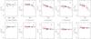 |
Fig. A.1
Statistical properties of 60 artificial, circular, Gaussian sources inserted into the raw time signals before data reduction a) to e) or directly inserted into the final unsmoothed continuum emission map of Cha I f) to j). a) and f): ratio of output to input peak flux density as a function of input peak flux density. b) and g): ratio of output to input peak flux density as a function of input size (FWHM). c) and h): ratio of output major size to input size as a function of input size. d) and i): ratio of output minor size to input size as a function of input size. e) and j): ratio of output to input total flux as a function of input size. The size of the black symbols scales with the input size of the sources. In addition, crosses and plus symbols are for input peak flux densities below and above 150 mJy/19.2″-beam, respectively. The red circles in panels b) to e) and g) to j) show a fit to the data points using the arbitrary 3-parameter function y = log (α / (1 + (x / β)γ)). |
| Open with DEXTER | |
Since LABOCA is a total-power instrument used without wobbler, the standard data reduction relies on the correlated signal of all pixels and of smaller groups of pixels to estimate and remove the atmospheric and instrumental noise. This method acts as a high-pass filter and makes the detection of very extended structures extremely difficult. The strongest limiting factor is the size of the groups of pixels connected to the same read-out cable (about 1.5′ by 5′, see Schuller et al. 2009). To analyse the dust continuum emission map in detail, it is therefore essential to understand the properties of this spatial filtering.
We performed several Monte Carlo simulations to characterize the filtering. First, we inserted artificial, circular, Gaussian sources in the raw time signals with the BoA method addSource after calibration. The sources were inserted at random positions in signal-free regions of the map shown in Fig. 2. The peak flux densities and FWHM sizes of the sources were randomly assigned in the range 50 to 500 mJy/beam and 19.2″ to 8′, respectively. The only constraint was that the artificial sources should not overlap and should not be too close to the map edges either. The modified raw data were then reduced following exactly the same procedure as described in Sect. 3.1, except that the final map was not smoothed and kept its original angular resolution of 19.2″ (HPBW). Each artificial source was fitted with an elliptical Gaussian using the task GAUSS_2D in GREG to measure its output peak flux density and sizes after data reduction. We also measured the total output flux on a circular aperture of radius equal to FWHM.
The whole procedure was repeated twice, with two independent samples of 30 artificial sources. Figures A.1a–e present the results. As a control check, we show in Figs. A.1f–j the results of the fits performed on the artificial sources directly inserted in the final unsmoothed continuum emission map of Cha I. The effects of the spatial filtering due to the data reduction are obvious when comparing Figs. A.1b–e to Figs. A.1g–j. The noise produces a small dispersion in the output source properties, especially for weak sources (crosses) but apart from that, all curves are basically flat in the control sample (Figs. A.1f–j). On the contrary, after data reduction, the peak flux densities of the sources are reduced by ~15% to ~70% for input sizes varying from ~240″ to ~440″. Similarly, the sizes of the sources are reduced by ~15% to ~50% for input sizes from ~200″ to ~440″. The total fluxes suffer the most from the spatial filtering: they are reduced by ~15% to ~90% for input sizes from ~120″ to ~440″. A careful inspection of Figs. A.1g–j shows that the sources with a peak flux density weaker than ~150 mJy/beam (crosses) are systematically below the stronger sources (plus symbols) for source sizes larger than ~100″. This is because the insertion of the stronger sources in the astronomical source model used for iterations 1 to 20 helps to recover more astronomical signal when their outer parts start to reach the thresholds mentioned in Sect. 3.1. The spatial filtering is therefore less severe for strong sources than for faint sources. These results are summarized in Table A.1.
A further Monte Carlo test was performed with elliptical Gaussian sources with a fixed aspect ratio of 2.5. The procedure to generate these artificial sources was the same, with the orientation of the sources also assigned randomly. The peak flux densities ranged between 85 and 500 mJy/beam and the size along the minor axis (FWHM) between 19.2″ and 3.7′. Three sets of sources were analysed, providing a sample of 68 sources in total. The results are very similar to the circular case, but with characteristic scales of the filtering along the minor axis of the elliptical sources 20–25% smaller (see Table A.1). In return, the corresponding characteristic scales of the filtering along the major axis are a factor of 2 larger than in the circular case. The peak flux densities are reduced by ~15% to ~20% for input sizes along the minor axis varying from ~180″ to ~220″ (i.e. sizes from ~450″ to ~550″ along the major axis). The aspect ratio is well preserved within ~10% after the last iteration, but the sizes of the sources are reduced by ~15% to ~25% for input sizes along the minor axis from ~160″ to ~220″ (i.e. from ~400″ to ~550″ along the major axis). Here again, sources with a peak flux density higher than ~150 mJy/beam are better recovered than weaker sources that cannot or can only partly be incorporated into the astronomical source model used at iterations 1 to 20.
These two Monte Carlo tests clearly show that the reduction of LABOCA data based on correlations between pixels to reduce the atmospheric and instrumental noise can have a strong impact on the structure of the detected astronomical sources. Depending on their shape and strength, structures with (major) sizes larger than ~140″–280″ if circular or ~300″–550″ if elliptical with an aspect ratio of 2.5 are significantly filtered out (>15% losses of peak flux density and size). Elongated structures are better recovered than circular ones. We note that the reduction performed for data obtained at the Caltech Submillimeter Observatory (CSO) with the bolometer camera Bolocam suffers from the same problem, with a similar characteristic scale above which losses due to spatial filtering start to be significant (~120″ for circular sources, see Enoch et al. 2006).
Several attemps to attenuate the correlated noise removal by using the outer pixels only, or to suppress the correlated noise removal and replace it subscan-wise with a simple first-order baseline removal in the time signals of the OTF scans, were not successful. These alternative reduction schemes produced somewhat more extended emission in places where we expected some, but at the same time, there were much more atmospheric and instrumental noise residuals distributed within the map that also mimicked extended structures where we did not expect any, by comparison to the extinction and C18O 1–0 maps for instance. Attempts to reduce the data without flattening the power spectrum at low frequency or with a lower cutoff frequency did not bring any significant improvement either.
A.2. Convergence of the iterative data reduction
The iterative process of data reduction described in Sect. 3.1 allows to recover additional astronomical flux after each iteration. In this section, we study the convergence of this method. The evolution of the total 870 μm flux recovered in Cha I as a function of iteration is shown in Fig. A.2a. The relative flux variation is only 0.7% at iteration 20, which suggests that the data reduction process indeed converged.
Filtering of artificial Gaussian sources due to the correlated noise removal depending on the input size along the minor (major) axis (FWHM).
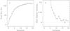 |
Fig. A.2
a) Convergence of the total 870 μm flux recovered in Cha I by the iterative process of data reduction. b) Relative flux variation between iterations i and i − 1 as a function of iteration number i. |
| Open with DEXTER | |
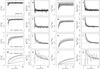 |
Fig. A.3
Convergence of the iterative data reduction for artificial, circular, Gaussian sources with a peak flux density larger than 150 mJy beam-1. The first and second columns show the ratio of the output to the input peak flux densities, and its relative variations, respectively. The third and fourth columns show the same for the total flux. The different rows show sources of different widths, as specified in each panel of the first column. The size of the symbols increases with the input peak flux density. |
| Open with DEXTER | |
This experiment shows that a significant number of iterations (about 20) are necessary to recover as much extended emission as possible. Enoch et al. (2006) have a similar conclusion with Bolocam for circular sources with FWHM < 120″ (convergence at iteration 5, see their Fig. 4), but they do not mention or show how many iterations they need to reach convergence17 for much larger sources.
Appendix B: Assumptions
In this Appendix, we explain the various assumptions that are used to analyse and interpret the Cha I data. We also explain how the column densities and average densities obtained in the past for other molecular clouds are rescaled in the present study to compare with Cha I (Table 7).
B.1. Distance
Whittet et al. (1997) analysed the distribution of extinctions of field stars with distance along the line of sight of Cha I and derived a distance of 150 ± 15 pc for this cloud. They also deduced a photometric distance for the B-type star HD 97300 of 152 ± 18 pc. They combined these results with the parallaxes of this and another star (HD 97048) measured with the Hipparcos satellite with a larger uncertainty (190 ± 40 and 180 ± 20 pc, respectively) and adopted a “final” distance of 160 ± 15 pc.
Knude & Høg (1998) used the interstellar reddening from the Hipparcos and Tycho catalogues to derive the distance to Cha I. They found a distance of 150 pc as revealed by a sharp increase in their plot of E(B − V) color excess versus distance.
However, Knude (2010) recently derived a further distance of 196 ± 13 pc for Cha I from a fit to an extinction vs. distance diagram. The extinction was obtained from a (H–K) vs. (J–H) diagram from 2MASS and the distances were estimated from a (J–H)0 vs. MJ relation based on Hipparcos. Rather than considering the distance at which the first stars show a steep increase in extinction as the distance of the cloud, they fitted a predefined function to a subsample of the data. It is unclear to us whether this fitting procedure does give a more reliable distance estimate because the selection of the subsample defining the extinction jump for the fit may introduce a bias. Therefore, as long as this further distance has not been confirmed by another method, we keep the older estimate (150 pc) as the distance of Cha I. If the further distance turns out to be correct, then all physical sizes and masses derived in this article are underestimated by a factor 1.3 and 1.7, respectively, and the mean densities are overestimated by a factor 1.3. The column densities are not affected.
B.2. Temperature
Tóth et al. (2000) derived a dust temperature of 12 ± 1 K for the “very cold cores” they identified in Cha I on somewhat large scales (HPBW ~ 2′) from their analysis of the ISOPHOT Serendipity Survey (see cores 1 to 6 in their Table 2). The dust temperature is most likely not uniform and this value rather represents a mean temperature. The dust temperature is expected to decrease toward the center of starless dense cores that do not contain any central heating, even down to ~5.5–7 K as measured for the gas in the prestellar cores L1544 and L183 by Crapsi et al. (2007) and Pagani et al. (2007), respectively. The modeled dust temperature profiles of the prestellar cores L1512, L1689B, and L1544 derived by Evans et al. (2001) indeed vary from 12–13 K in the outer parts to 7–8 K at the core center. Similarly, Nutter et al. (2008) measured a dust temperature varying from 12 K in the outer parts to 8 K in the inner parts of a filament in the Taurus molecular cloud 1 (TMC1). Thanks to its good angular resolution and its good sampling of the spectral energy distribution of these cores, such temperature variations will be routinely measured in the far-infrared with the Herschel satellite, which will help refining the mass and column density estimates (see, e.g., André & Saraceno 2005). For simplicity, we assume here a uniform dust temperature of 12 K.
If the temperature inside the dense cores drops to, e.g., 7 K, their masses and column densities computed in this article could be underestimated by up to a factor of 3, depending on the exact shape of the temperature profile. However, the total mass of a core being dominated by its outer parts, it should not be that much underestimated.
B.3. Conversion of visual extinction to H2 column density
The standard factor to convert a visual extinction AV to an H2 column density is 9.4 × 1020 cm-2 mag-1. It is based on the ratio NH / E(B − V) = 5.8 × 10²¹ atoms cm-2 mag-1 measured by Bohlin et al. (1978) with data from the Copernicus satellite, and a ratio of total-to-selective extinction RV = AV / E(B − V) = 3.1 corresponding to the standard extinction law that is representative of dust in diffuse regions in the local Galaxy (see, e.g., Draine 2003,and references therein).
Several measurements suggest that RV is larger toward denser molecular clouds. In particular, Chapman et al. (2009) computed the mid-IR extinction law based on Spitzer data in the three molecular clouds Ophiuchus, Perseus, and Serpens and found indications of an increase of RV from 3.1 for AKs < 0.5 mag to 5.5 for AKs > 1 mag, which they interpret as evidence for grain growth. Using the parameterized extinction law of Cardelli et al. (1989, their Eqs. (1), (2a), and (2b)) with RV = 3.1 and 5.5, respectively, we find that these two thresholds correspond to AV < 4.2 mag and AV > 7.2 mag. Vrba & Rydgren (1984) came to a similar conclusion for Cha I since they found a standard extinction law toward the outer parts of the cloud but reported a larger RV (>4) for field stars near the denser parts of the cloud (see also Whittet et al. 1994). Therefore, we assume that the thresholds derived by Chapman et al. (2009) also apply to Cha I. With RV = 5.5, the factor to convert a visual extinction into an H2 column density becomes 6.9 × 1020 cm-2 mag-1 (see Evans et al. 2009,and references therein). However, the visual extinction values presented here are derived from near-infrared measurements assuming the standard extinction law (RV = 3.1). Compensating for this assumption, the “corrected” conversion factor for RV = 5.5 mag becomes NH2 / AV = 5.8 × 1020 cm-2 mag-1 for our extinction map calibrated with RV = 3.1.
In summary, for AV below ~6 mag in our extinction map we assume RV = 3.1 and the standard conversion factor NH2 / AV = 9.4 × 1020 cm-2 mag-1. For AV above ~6 mag, we assume RV = 5.5 and NH2 / AV = 5.8 × 1020 cm-2 mag-1.
B.4. Dust mass opacity
The dust mass opacity in the submm range is not well constrained and is typically uncertain by a factor of 2 (e.g. Ossenkopf & Henning 1994). Since most sources detected in the survey of Cha I are weak, starless cores, we adopt a dust mass opacity, κ870, of 0.01 cm2 g-1 in most cases (and a dust opacity index β = 1.85). It corresponds to the value recommended by Henning et al. (1995) for “cloud envelopes”, assuming β ~ 1.5–2.0 and a gas-to-dust mass ratio of 100. For higher densities (nH2 ~ 5 × 106 cm-3) that characterize the inner part of a few sources in our survey, κ870 is most likely higher, on the order of 0.02 cm2 g-1 (Ossenkopf & Henning 1994). Finally, the dust mass opacity in circumstellar disks is expected to be even higher. We follow Beckwith et al. (1990) with β = 1 and derive κ870 = 0.03 cm2 g-1 for this type of sources. In the article, we each time specify which dust mass opacity we use to compute column densities and masses. We assume in all calculations that the dust emission is optically thin.
B.5. Molecular weight
The mean molecular weight per hydrogen molecule and per free particle, μH2 and μ, are assumed to be 2.8 and 2.37, respectively (see, e.g., Kauffmann et al. 2008). The former is used to convert the flux densities to H2 column densities while the latter is needed to estimate the free-particle densities.
B.6. Rescaling of previous results on other clouds
B.6.1. Column densities
Assuming a temperature of 10 K and a dust mass opacity of κ1.1 mm = 0.0114 cm2 g-1, Enoch et al. (2008) derive average peak H2 column densities of 1.2 and 1.0 × 1022 cm-2 in Perseus and Serpens, respectively. Their values have to be multiplied by 1.3 to match the same properties as we use for Cha I (12 K, β = 1.85 yielding κ268 GHz = 0.0063 cm2 g-1). In addition, both clouds are at larger distances than Cha I and the Bolocam maps have a poorer angular resolution (31″) compared to our LABOCA map (21.2″). If the sources in Perseus and Serpens are not uniform in the Bolocam beam but rather centrally peaked with a column density scaling proportionally to the inverse of the beam size, then their peak column densities measured in the same physical size as for Cha I would be about 2.4–2.5 times larger. The full rescaling factor is thus 3.1–3.5. We rescale the average column density of the SCUBA starless cores analysed by Curtis & Richer (2010) in Perseus in the same way (12 K and κ353 GHz = 0.010 cm2 g-1), after correction for a small error18 in their numerical Eq. (5). The column density is also rescaled proportionally to the inverse of the beam size. The rescaled values of both studies of Perseus are consistent.
The average peak column density of the Bolocam starless cores observed by Enoch et al. (2008) in Ophiuchus was rescaled in the same way as above. The average peak column density derived for the starless cores of Motte et al. (1998) after rescaling to the same physical size as for the Cha I sources with an Ophiuchus distance of 125 pc is a factor of ~2 lower. The discrepancy between both studies may come from the background emission not being removed in the former study, from the assumption of a unique temperature for all sources in the former study while the second one uses different temperatures (from 12 to 20 K), and from our assumption of a column density scaling with the inverse of the radius.
Kauffmann et al. (2008) analysed their maps
of Taurus after smoothing to 20″, i.e. nearly the same spatial resolution as our
Cha I map given also the slightly different distances. Their column density
sensitivity is similar to ours. Assuming the same dust properties as for Cha I
(Tdust = 12 K and β = 1.85 yielding
κ250 GHz = 0.0055 cm2 g-1),
the average column density in an aperture of 20″ derived from the flux densities
listed in their Table 5 is  cm-2
for their sample of 28 Taurus starless “peaks”.
cm-2
for their sample of 28 Taurus starless “peaks”.
B.6.2. Densities
Enoch et al. (2008) obtain average densities of 1.7, 1.4, and 2.8 × 105 cm-3 within an aperture of diameter 104 AU for the starless cores in Perseus, Serpens, and Ophiuchus, respectively. We assume a density profile proportional to r − p with p ~ 1.5–2, which is typical for such cores, and rescale their densities with a temperature of 12 K and a dust opacity κ268 GHz = 0.0063 cm2 g-1.
With the same assumptions as in Sect. B.6.1,
the 28 starless “peaks” of Kauffmann et al.
(2008) in Taurus have an average mass of
 M⊙
within an aperture of diameter 8400 AU. We assume the same density profile as above
to compute the average mass within an aperture of diameter 7500 AU and derive the
average density.
M⊙
within an aperture of diameter 8400 AU. We assume the same density profile as above
to compute the average mass within an aperture of diameter 7500 AU and derive the
average density.
Appendix C: Multiresolution decomposition
As mentioned in Sect. 1.5.1 of Starck et al. (1998), multiresolution tools based on a wavelet transform suffer from several problems, in particular they create negative artefacts around the sources. In addition, since the emission is smoothed with the scaling function (Φ) to produce the large-scale planes, the shape of the large-scale structures is not preserved and tends toward the shape of Φ (which, in turn, creates the negative artefacts in the small-scale planes mentioned above). For instance, a circularly symmetric filter will tend to produce roundish structures on large scale. To avoid these issues, we performed a multiresolution analysis based on the median transform following the algorithm of Starck et al. (1998, Sect. 1.5.1) that we implemented in Python. In short, the input image is first “smoothed” with a filter that consists of taking the median value on a 3 × 3-pixel grid centered on each pixel. The difference between the input and smoothed images yields the “detail” map at scale 1 (the smallest scale). The same process is repeated with a 5 × 5-pixel grid
using the smoothed map as input map, and the difference between the two images produces the detail map at scale 2. The process is done 7 times in total, yielding detail maps at 7 different scales. The size of the convolution grid at scale i is n × n pixels with n = 2i + 1, i.e. 18.3″, 30.5″, 54.9″, 1.7′, 3.4′, 6.6′, and 13.1′ for scales 1 to 7, respectively. The last smoothed map contains the residuals (very large scale). The sum of the residual map and the 7 detail maps is strictly identical to the input map.
Characteristics of the multiresolution decomposition as measured on a sample of circular and elliptical artificial Gaussian sources with a signal-to-noise ratio higher than 9.
The properties of this multiresolution decomposition were estimated with the samples of
artificial Gaussian sources of Appendix A.1 (both
circular and elliptical with aspect ratio 2.5) inserted into the reduced continuum map
of Cha I. Table C.1 presents the results for
sources with a signal-to-noise ratio higher than 9. For each scale i,
the artificial sources were fitted in the map containing the sum of the detail maps from
scale 1 to i (hereafter called sum map at scale
i). Compact sources (FWHM < 30″) are fully
recovered at scale 4 while sources with FWHM > 120″ are strongly
filtered out (losses >60%). Therefore, scale 4 is a good scale to extract compact
sources when they are embedded in larger scale cores (>120″). Similarly, scale 5
is a good scale to extract sources with FWHM < 120″ with an
accuracy better than 20% on the peak flux density, while significantly filtering out the
more extended background emission (losses >60% for
FWHM > 200″). In the case of the elliptical sources with aspect
ratio 2.5, the conclusions are the same, the key parameter being the geometricalmean of
the sizes along the major and minor axes ( ).
).
© ESO, 2011
Current usage metrics show cumulative count of Article Views (full-text article views including HTML views, PDF and ePub downloads, according to the available data) and Abstracts Views on Vision4Press platform.
Data correspond to usage on the plateform after 2015. The current usage metrics is available 48-96 hours after online publication and is updated daily on week days.
Initial download of the metrics may take a while.