| Issue |
A&A
Volume 708, April 2026
|
|
|---|---|---|
| Article Number | A350 | |
| Number of page(s) | 12 | |
| Section | Galactic structure, stellar clusters and populations | |
| DOI | https://doi.org/10.1051/0004-6361/202557853 | |
| Published online | 23 April 2026 | |
Luminosity functions and initial mass function variations from large samples of H II regions and molecular clouds
1
Laboratoire d’Astrophysique de Bordeaux, Univ. Bordeaux,
CNRS, B18N, allée Geoffroy Saint-Hilaire,
33615
Pessac,
France
2
INAF-Osservatorio Astrofisico di Arcetri,
Largo E. Fermi, 5,
50125
Firenze,
Italy
★ Corresponding authors: This email address is being protected from spambots. You need JavaScript enabled to view it.
; This email address is being protected from spambots. You need JavaScript enabled to view it.
Received:
27
October
2025
Accepted:
16
March
2026
Abstract
Large high-quality samples of HII regions and their parent giant molecular clouds (GMCs) are now available for local galaxies. It is therefore possible to investigate the links between the CO and Hα luminosity functions and whether massive stars form in GMCs of all masses. The CO luminosity functions, representing the distribution of GMC masses, are consistently steeper than the Hα luminosity functions. The CO luminosity function invariably steepens in the outer disk, where fewer massive GMCs are present beyond the median cloud galactocentric distance. The Hα luminosity function also steepens in the outer disk for most of the galaxies examined. Using Salpeter, Kroupa, and Chabrier initial mass functions (IMFs) along with stellar mass-luminosity-radius relations, we calculate the bolometric luminosity and Hα emission from young star clusters. The cluster masses are linked to the GMC mass by assuming that the cluster mass is a constant fraction (3%) of the parent cloud mass. In particular, results for a fully stochastic IMF are compared to suggestions that very massive stars only form in massive clusters or clouds. Within the limits of the observations - no small molecular clouds or low-luminosity HII regions can be detected at the typical ∼10 Mpc distance of the sample galaxies - we find no evidence for a maximum stellar mass that varies with cloud or cluster mass.
Key words: HII regions / ISM: molecules / open clusters and associations: general / galaxies: ISM / galaxies: spiral / galaxies: star formation
© The Authors 2026
 Open Access article, published by EDP Sciences, under the terms of the Creative Commons Attribution License (https://creativecommons.org/licenses/by/4.0), which permits unrestricted use, distribution, and reproduction in any medium, provided the original work is properly cited.
This article is published in open access under the Subscribe to Open model. This email address is being protected from spambots. You need JavaScript enabled to view it. to support open access publication.
1 Introduction
The large samples of HII regions and giant molecular clouds (GMCs) now available should tell us something about the stellar initial mass function (IMF). In particular, is the IMF the same for large and small GMCs? It is commonly accepted that stars, and thus HII regions, form in GMCs. If small GMCs do not form massive stars, i.e. they do not populate the upper end of the stellar mass distribution, then this should be visible in the HII region luminosity function. This is the main subject of this short contribution.
As in previous works, we assume that the intrinsic shape of the GMC mass distribution (or function) is that of a power law N(m)dm ∝ m-αdm, with or without truncation at the high-mass end (Solomon et al. 1987; Rosolowsky et al. 2007; Gratier et al. 2012; Colombo et al. 2014; Braine et al. 2018; Rosolowsky et al. 2021). When the index of the mass (or luminosity) function is steeper than α = 2, then most of the mass is in the small entities. The lifetimes of the massive stars creating H II regions are quite short so large samples are required to sample all phases (ages) of young stellar clusters.
While the stellar IMF seems fairly constant in today’s spiral disks, it appears to be increasingly accepted that the IMF in low-metallicity or extremely dense environments is different (Larson 1998; Kroupa 2001; Hopkins 2018). The change is likely a shift in the characteristic (i.e. average) mass Mchar of low-mass stars. This would not change the formation process of massive stars and hence leave the slope of the high-mass part of the IMF unchanged (Hopkins 2018). The core Jeans mass would increase due to a lower metal (dust) content or to factors inhibiting fragmentation (e.g., tidal forces). Increasing Mchar means that a smaller fraction of the gas converted into stars goes into low-mass stars, raising the luminosity-to-mass ratio (L/M) of the cluster.
In this work we compare the GMC luminosity function with the H II region luminosity function in local spiral galaxies. GMCs and HII regions are respectively traced by the CO(2-1) and Hα lines. The CO luminosity is generally used as an equivalent of cloud mass. Since the range in HII region or GMC luminosity between completeness and a possible truncation at the high-mass end is often small, considerable attention will be paid to the fitting.
The lifetime of a GMC tGMC, that is to say the time during which it is recognizable as a GMC, is of order 15 Myr (Gratier et al. 2012; Corbelli et al. 2017; Calzetti et al. 2012; Chevance et al. 2020; Kobayashi et al. 2017; Demachi et al. 2024). At a galactic scale, the H2 depletion time tdepl = M(H2)/SFR, where "SFR" is the star formation rate in solar masses per year, is about 2 × 10⁹ yr (Murgia et al. 2002; Leroy et al. 2013). Similarly, SFR = εSFM(H2)/tGMC so, averaged over the whole star formation cycle, the fraction of the gas turned into stars is about εSF = tGMC/tdepl ≈ 1%. Within the gas sufficiently dense to be identified by cloud-finding algorithms (typically a few times the rms noise), the efficiency (εSF) appears to be higher, some 23% (Murray 2011; Evans et al. 2009), and the difference can be explained by the fact that roughly half of the gas detected at galactic scales is not locked into individual clouds because it is too diffuse and does not emit strongly enough in the CO lines.
Larson (2003) found that the mass of the most massive star of a cluster increased with the mass of the star cluster roughly as  . For a given εSF, this suggests that the stellar mass range in a cluster depends on the GMC mass and indeed the original study by Larson (1982) found
  . For a 10 000 M⊙ cloud, the IMF would be truncated at ∼20 M⊙ in this scenario. A similar scenario, also limiting the production of high-mass stars in small clusters, was proposed by Weidner & Kroupa (2006). As a result of either of these scenarios, a galaxy would have fewer massive stars than predicted by the IMF because low-mass GMCs would not contribute to the high-mass star population. On the other hand, if the IMF is stochastically sampled, then although the birth of a massive star is less likely in a low mass cluster, they would occasionally form and the overall IMF would be preserved (Corbelli et al. 2009; da Silva et al. 2014). The CO and Hα data used here enable us to examine possible links between cloud mass and the mass of the most massive star formed because the Hα luminosity of a cluster, particularly a small cluster, depends strongly on the mass of the most massive star remaining.
Large homogeneous high-quality samples of Hα and CO observations of individual clouds and H II regions in nearby galaxies have only recently become available. The PHANGS (Physics at High Angular resolution in Nearby GalaxieS Leroy et al. 2021) survey has made public the CO and Hα luminosities for large samples of GMCs (Rosolowsky et al. 2021) and H II regions (Santoro et al. 2022) in the galaxies of their sample. As the overlap of the CO and Hα samples is small (2 galaxies), we add data for the Local Group galaxy M33 as outlined below in Section 2. Section 3 describes how we link cloud masses to young stellar cluster masses and to populations of individual stars and their properties, along with the fitting methods. In Sect. 4, we compare the results of the fits to the H II region and cloud luminosity functions for the inner and outer parts of the galactic disks. The distributions of GMC luminosities are systematically steeper than those of HII regions and Sect. 5 examines possible explanations and particularly whether introducing a stellar mass limit (Larson 1982; Weidner & Kroupa 2006) helps explain the results.
2 Samples
We selected galaxies with enough data to be suitable for statistical analyses. On average, the GMC and HII region samples have about 700 GMCs and 1000 HII regions per galaxy, as described below. With the exception of M33, the resolutions of the CO and Hα observations are similar (see Table 2 of Rosolowsky et al. (2021) and Table 1 of Santoro et al. 2022). However, in all cases, we use the catalogs produced from the observations by the observers.
2.1 Molecular clouds
As part of the PHANGS collaboration (e.g., Schinnerer et al. 2019), a large catalogue of GMCs observed with ALMA was published and made public by Rosolowsky et al. (2021). The catalog presents data for 10 galaxies but we do not include data for two small galaxies because they have too few clouds (less than 100) to determine a mass function. The eight remaining galaxies are large spirals with effective radii between 2.6 and 4.1 kpc and have between 275 and 1432 clouds (over 5000 for the eight galaxies, see Table 5 of Rosolowsky et al. 2021).
We added data for the local group spiral M33 (Druard et al. 2014; Corbelli et al. 2017) for which both CO and Hα data are available. Basic information on the galaxies can be found in Table 1 of Rosolowsky et al. (2021) and in Table 1 of Druard et al. (2014) for M33.
2.2 H II regions
Also as part of PHANGS, a large (>20 000) catalog of HII regions observed with MUSE was published and made publicly available by Santoro et al. (2022). They observed 19 galaxies with 472-2536 HII regions identified per galaxy. Basic information on the galaxies can be found in Tables 1 and 2 of Santoro et al. (2022). The distances and angular and physical resolutions of the observations are similar to those of Rosolowsky et al. (2021). However, despite being part of the PHANGS sample as well, only two galaxies were observed in common between the catalogs. Adding M33 Hα data from Lin et al. (2017) provides a third galaxy in common.
By fitting power laws to the distribution of Hα luminosities for each galaxy, Santoro et al. (2022) found that the spectral index α may decrease (flatten) with increasing galaxy-averaged star formation rate surface density. The range in α was from 1.52 to 2.04 with formal uncertainties of about 0.1. After identifying spiral and interarm regions, Santoro et al. (2022) found that α is steeper in the interarm. They did not find a change in α between the inner and outer parts of the galaxies, unlike what was found for GMCs by Gratier et al. (2012) and Rosolowsky (2005), raising the question of why would (or how could) the H II region and GMC distributions be different. We noticed that the spectral index α depended on the minimum luminosity deduced by the powerlaw.py algorithm they used (Alstott et al. 2014), motivating us to investigate this issue further (see Sect. 3.5).
3 Stellar properties and methods
3.1 The stellar IMF
There are three widely studied IMFs - the original Salpeter (1955) IMF with the number of stars formed per interval of mass, n(m) ∝ m−α and α = 2.35, the Kroupa (2001) disjoint IMF where α = 1.3 for masses between 0.08 and 0.5 M⊙ but α = 2.35 for larger masses, and the Chabrier (2003) IMF which is lognormal (see their Eq. (17)) up to 1 M⊙ and Salpeter for higher masses. Wherever relevant, we assume stellar masses range from 0.08 to 100 M⊙. In practice, we use this in logarithm so n(m) = dn/dm becomes (per logarithmic mass interval)
dn/d(ln(m)) = mdn/dm, yielding
dn/d(ln(m)) ∝ m−1.35 for the Salpeter (1955) IMF,
dn/d(ln(m)) ∝ m−0.3 for M < Mchar (Kroupa 2001), and
 for M < 1 M⊙ (Chabrier 2003). All of these IMFs have the same (Salpeter) distribution for stars with masses higher than the limiting values quoted above.
The distributions are shown in Figure 1. Integrating these functions from 0.08 to 100 M⊙ yields average stellar masses of 0.28, 0.54, and 0.58 for the Salpeter, Kroupa, and Chabrier IMFs, respectively.
3.2 From stellar masses to luminosities
The zero-age light-to-mass ratios, for a complete sampling, are respectively 191, 278, and 298 L⊙/M⊙ for the three IMFs assuming a simple scaling of L ∝ M3. Two more complicated but more realistic mass-luminosity relations (MLR) were also used. The first has L ∝ M2.3 for M < 0.43 M⊙, L ∝ M4 for 0.43 < M < 2 M⊙, L ∝ M3.5 for 2 < M < 55 M⊙, and L ∝ M for M > 55 M⊙ approximately following Eker et al. (2015). With this MLR, the zero-age light-to-mass ratios become 1240, 1790, and 1940, respectively. The second MLR uses Eker et al. (2018) Table 6 followed by Sternberg et al. (2003) for the higher masses. The main difference is that this MLR has slightly lower temperatures and luminosities for the highest masses, yielding zero-age light-to-mass ratios of 635, 918, and 993 L⊙/M⊙, respectively. Since this difference between the two MLRs comes from the most short-lived stars, it decreases greatly over the first megayear. The reader is referred to the Appendix for the details of the (IMF and) MLR.
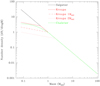 |
Fig. 1 Initial mass functions used in this work. Black line is for Salpeter, red is for Kroupa, and green is for the Chabrier IMF. The plot shows the number of stars per logarithmic mass interval for each mass. Clearly, the Kroupa and Chabrier IMFs are similar and have significantly fewer low-mass stars than the Salpeter IMF. The dashed and dotted lines show the Kroupa IMF using somewhat higher characteristic masses. The effect of increasing the characteristic mass is that there are fewer low mass stars so the L/M ratio of the stellar population increases from about 900 L⊙/M⊙ to 1500 L⊙/M⊙. |
3.3 Populating stellar clusters
The standard procedure to randomly sample the IMF is to calculate the cumulative distribution functions of each IMF, normalize to unity, draw random numbers uniformly between zero and one, and then take the star mass associated with that value of the cumulative distribution function. Stellar clusters are built up to a given mass. In practice the mass is slightly greater (generally less than 1%) than the nominal cluster mass because we draw stars as long as the mass is below the nominal cluster mass. This is reasonable, as the cluster masses are far below the cloud masses, so there is still a large reservoir of material left to form stars. Random sampling results in huge luminosity variations, particularly before aging, as cluster luminosities can be dominated by a single star. Drawing a large number of stellar clusters naturally yields average values of the luminosities close to those calculated by directly integrating the IMF and applying the MLR. Clusters are populated once a cluster mass has been chosen, typically 3% of the cloud mass, and the process is independent of the cluster or cloud mass. To obtain a GMC mass distribution typical of the galaxies sampled in this paper, we assume that GMC masses follow a power law with α = 2, unless otherwise stated. This is the average value for the GMC distribution in PHANGS galaxies, but we also show results for α = 1.7 and α = 2.3 to illustrate the possible effects of changing the slope of the mass distribution.
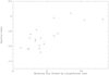 |
Fig. 2 Link between spectral index measured with powerlaw.py and Lmin for the 19 galaxies from data given in Table 2 of Santoro et al. (2022). Lmin is normalized by the completeness limit Lcompl to be comparable from one galaxy to another. |
3.4 Randomness” of star formation
When populating a stellar cluster by randomly sampled stellar masses following a given IMF, cluster-to-cluster luminosity variations (bolometric and Hα) can be quite high, dependent on the mass of the most massive star. This is illustrated in Fig. A.2 for 1000 simulations of clusters of ∼300 M⊙. If ∼3% of a cloud is turned into stars, a 300 M⊙ stellar cluster corresponds to an initial cloud mass of ∼ 10 000 M⊙, which is approximately the lower limit to what is considered a GMC. Zero-age luminosities of a 300 M⊙ cluster vary by more than a factor of 1000, depending on the presence of a massive star or not, and the dispersion in luminosities is comparable to the average luminosity, such that for a sample of 100 clusters, major variations can be present due to the stochastic sampling of the IMF.
For truly massive clusters, this effect becomes small although not negligible even for clusters of 10 000 M⊙ of stars, as many massive stars are present. This fact is taken into account in our simulations.
3.5 Algorithms
After reproducing the results presented in Figure 2 of Santoro et al. (2022), we tested the influence of the Lmin parameter and indeed found that for a given galaxy, increasing Lmin above Lcompl yielded a systematically steeper slope. This is not only true for the powerlaw.py algorithm but also for the algorithms used by Rosolowsky et al. (2021) (see their Table 5). Figure 2 shows how the spectral index of the galaxies depends on Lmin normalized to the completeness limit Lcompl, both given in their Table 2. When data have a physical high-end truncation coupled with increasing incompleteness at low fluxes, this behavior is expected and it represents one of the difficulties in fitting.
The powerlaw.py (Alstott et al. 2014) algorithm searches for an “optimal” Lmin without knowledge of Lcompl but it can also be used with a fixed Lmin. For each galaxy in the MUSE and ALMA samples, we ran multiple powerlaw.py fits testing many values of Lmin bracketing Lmin and Lcompl. While the change in slope was generally large and regular, the relative slopes between the inner and outer parts changed little. The fact that power-law.py does not use knowledge of Lcompl, which depends on the sensitivity of the observations, is a drawback for experimental data. Alstott et al. (2014) illustrate the powerlaw.py algorithm with word occurrence and blackout statistics that do not have a sensitivity (completeness) limit, although powerlaw.py allows a minimum value to be injected. Our approach has been to use an Lmin based on Lcompl. We adopted Lmin = 2Lcompl for the Santoro data and equal to Lcompl for the other data.
We tried fitting using a least-squares algorithm to both the luminosities and their logarithms but this yielded visually inappropriate results. The algorithm used by Rosolowsky et al. (2021) yielded extremely large variations in α for only modest changes in Lmin (completeness in their Table 5) so this was not investigated further.
Gratier et al. (2012) used an algorithm based on the work by Maschberger & Kroupa (2009). This was tested on the current CO and Hα data with reasonable results, generally similar to powerlaw.py for similar Lmin. Figures 3 and 4 present results using both the powerlaw.py algorithm and the Maschberger & Kroupa (2009) technique. The Maschberger-Kroupa power-law fit uses a truncated power law. The powerlaw.py algorithm has no truncation.
Using simulated data taken from a power law distribution (α = 1.4,1.5...2.0) with random added noise, both the powerlaw.py and the Maschberger & Kroupa (2009) algorithms performed well. However, for a given noise level, the Maschberger & Kroupa (2009) did measurably better in recovering the initial distribution.
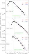 |
Fig. 3 Probability density functions of Hα fluxes from NGC0628, NGC3627, and M 33, the three galaxies for which both HII region and GMC catalogs are available. Results of the powerlaw.py (red line) and Maschberger & Kroupa (2009) (blue line) fits along with observational data for NGC0628, NGC3627, and M33 from Santoro et al. (2022) and Lin et al. (2017) are shown. NGC0628 and NGC3627 are the two PHANGS galaxies for which both the HII region and GMC samples are available. The Hα data for M33 are from Lin et al. (2017). The adopted completeness limit for the fits (equivalent of Lmin in Santoro et al. 2022) are shown as a dashed green line and given in Table 1 The error bars are proportional to |

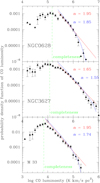 |
Fig. 4 Probability density functions of CO luminosities from NGC0628, NGC3627m and M33, the three galaxies for which both HII region and GMC catalogs are available. Results of powerlaw.py (red line) and Maschberger & Kroupa (2009) fit (blue line) along with observational data for NGC0628, NGC3627, and M33 from Rosolowsky et al. (2021) and Corbelli et al. (2017). NGC0628 and NGC3627 are the two PHANGS galaxies for which both the H II region and GMC samples are available. The CO data for M33 are from Druard et al. (2014) and Corbelli et al. (2017). The adopted completeness limits for the fits are the first of the limits given in Table 5 of Rosolowsky et al. (2021) and are shown as a dashed green line and given in Table 2. The error bars are proportional to |

Hα results for the PHANGS MUSE galaxies.
4 HII region and GMC luminosities across galaxy disks
We calculate the Probability Density Function (PDF) as the number of objects per bin divided by the bin width. For example, at log(CO luminosity) = 6 and for a bin width of 0.1 dex as in Fig. 4, the width is 2.3 × 10⁵, so if 20 objects are present, the PDF for that luminosity bin is 20/(2.3 × 105) = 8.7 × 10⁻⁵. Given that the PDFs are presented per galaxy, such that the distance to each region is the same, the shape of a flux PDF or a luminosity PDF is the same. The slope α of the fit to the PDF is the spectral index.
Figure 3 shows the PDF of the HII region Hα fluxes of NGC0628, NGC3627, and M33. The powerlaw.py fit is shown as a red line and the Maschberger & Kroupa (2009) fit is shown as a blue line. The assumed completeness level (used for both fits) is indicated with a dashed green line. These galaxies have been chosen because they are the only PHANGS galaxies for which both H II region and GMC catalogs are available. Figure 4 shows the results for CO luminosities of the same galaxies. It can be seen that the CO results are based on a significantly smaller dynamic range (ratio between completeness level and maximum) than the Hα flux distribution.
To fit the GMC distributions, we chose to use the lower completeness level given by Rosolowsky et al. (2021) in their Table 5 and reproduced in Table 2. The GMC slopes are clearly steeper than for the H II regions. The GMC completeness limit was originally given by Rosolowsky et al. (2021) as a mass so it was converted to a CO luminosity using their Eq. (5) for a solar metallicity. We use the CO luminosities because they are the observed quantities (whereas the mass requires a conversion factor) and directly comparable to the Hα luminosities. The fits were also performed using the masses in the online table with no significant difference. See Section 5.1 for a discussion of the effect of a change in N(H2)/ICO.
The fitting results are given in Table 1 for the H II regions and Table 2 for the GMC sample. The fits using the powerlaw.py algorithm (Alstott et al. 2014) and the Maschberger & Kroupa (2009) procedure are shown as αpy and αMK, respectively. The uncertainties are estimated via the bootstrapping method with 100 random draws for each fit. For the HII regions, we find 1.47 ≤ αpy ≤ 1.87 (average 1.64 and dispersion 0.10) and 1.42 ≤ αMK ≤ 1.86 (average 1.61 and dispersion 0.11). Linking the minimum flux used for the fits to the completeness level given in Table 2 of Santoro et al. (2022) results in a decrease of the dispersion from 0.15 to 0.10. For the GMCs, we find 1.65 ≤ αpy ≤ 2.98 (average 2.09 and dispersion 0.42) and 1.55 ≤ αMK ≤ 3.00 (average 2.14 and dispersion 0.39). The dispersion in α found by Rosolowsky et al. (2021) using different methods is considerably higher (1.14 and 0.44 from cols 3 and 6 of their Table 5) for the eight galaxies with more than 100 GMCs. Our two fitting methods are in good agreement for both the H II regions and the GMCs, showing that the average spectral index αCO > αHα. For the three galaxies in common, NGC 628 and NGC 3627 in the PHANGS sample and M33, the slope of the GMC PDF is also steeper than that of the H II region PDF, so it is likely a general feature.
Figure 5 illustrates the slopes and their radial variation. For each galaxy, with the galaxies that have both GMC and HII region data at the top, the CO index αCO is shown, followed by the HII region index αHα. Both fits are presented (triangles) and the horizontal bar is the average. When only a single triangle is visible, it simply means the agreement between the methods was excellent. The horizontal dotted line is a guide and shows a slope of 1.5, making it clear that the αCO are steeper then αHα. The following columns show how the spectral index, α, varies between the inner and outer parts. All CO luminosity functions become steeper, in agreement with previous work. A majority of the Hα luminosity functions steepen with radius but the trend is less consistent and has exceptions. Figure 6 illustrates the radial variation of α in a simpler fashion.
The general features are that (1) the CO luminosity functions are steeper than the Hα luminosity functions and (2) the distribution of CO luminosity steepens systematically in the outer parts, unlike the distribution of Hα luminosity. This result is independent of the fitting routine and of any reasonable choice of parameters so we must now explore possible reasons.
CO results for the PHANGS galaxies.
5 Why is αCO steeper than αHα ?
Intrinsically, for a given IMF, we expect that a cloud will convert some fraction (2-3%) of its mass into stars and hence create an HII region of a luminosity that should depend on the initial cloud mass. At some point the cloud will be dispersed by supernovae and winds. Thus one would expect, at least before the first supernova, that the slopes of the luminosity functions should be the same.
The GMC samples discussed here have cloud masses well in excess of 10000 M⊙. The HII regions are also quite luminous so we only discuss H II regions with initial stellar masses well in excess of the mass of an individual massive star, assumed to be ≤100 M⊙. While there are examples of star formation in low-mass clouds, in GMCs stars tend to form in dense cores (<pc), themselves within dense clumps (1-10 pc) within the GMC. The clouds studied here are GMCs ranging from 104 to over 106 M⊙, so clusters rather than individual stars are formed, and the mass reservoir is large even if only 3% of the GMC mass is converted into stars.
It appears that the power-law part of the IMF, i.e., beyond about 2 M⊙(see Fig. 1), is due to different processes and independent of whether the lower end follows a Salpeter, Kroupa or Chabrier distribution. A high local gas density and/or low metal-licity could push up the characteristic mass (manifested by the turnover of the Kroupa IMF) but would probably not affect the high-mass end (see discussions in Larson 1998; Kroupa 2001; Hopkins 2018). Since the HII region luminosity is completely dominated by the high-mass end of the IMF, these changes should not affect the link between cloud mass and HII region luminosity.
In the rest of this section we consider effects that complicate this picture, such as
The conversion from CO luminosity to H2 mass may not be constant.
The luminosity of a given H II region depends strongly on the mass of the most massive star such that a cluster containing 1000 M⊙ of stars drawn randomly can have a radically different luminosity depending on whether a truly massive star is “drawn.” This adds noise to the system and is why it is important to have many regions.
HII regions age quickly in that their population of massive stars changes significantly over the lifetime of a molecular cloud (∼15 Myr, approximately the lifetime of a O9 or B0 star).
The IMF could vary. An interesting proposal we are aware of is a link between the mass of the most massive star (M*,max) in the cluster and the parent molecular cloud mass as proposed by Larson (1982).
5.1 Variations of N(H2)/ICO with galactocentric radius
Metallicities tend to decrease with galactocentric radius, as do gas temperatures, and both tend to result in an increase of the N(H2)/ICO conversion further from galactic centers. The basis for the N(H2)/ICO factor is clearly presented in Dickman et al. (1986), and recent discussions of the N(H2)/ICO factor can be found in Teng et al. (2024), Schinnerer & Leroy (2024), and Leroy et al. (2025). We made tests by randomly choosing positions and drawing cloud CO luminosities with a predefined spectral index (α). We then added a radial N(H2)/ICO gradient to obtain cloud masses and processed the data like real data. The
Fits of the mock data.
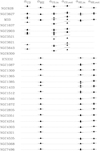 |
Fig. 5 Results of fits to the distribution of Hα and CO luminosities. For each galaxy, the name is indicated followed by (1) the whole-galaxy GMC spectral index; (2) the whole-galaxy Hα spectral index; (3) the inner and outer GMC spectral index, connected by a line; and (4) the same but or the Hα luminosities of HII regions. In each case, the triangles indicate the values obtained from the two independent fitting methods and the average is shown by the short horizontal line. When the line goes up, the distribution in the outer part is steeper (relatively more small objects). A horizontal dashed line at a value of 1.5 is plotted to allow easy appraisal of the values. |
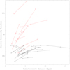 |
Fig. 6 Radial variation of spectral indices. This plot portrays the latter four columns of Fig. 5 in a simpler fashion. The lines start with the median position of the inner regions (H II or GMC) and end at the median position of the outer regions. The marker near the line center indicates the median galactocentric distance of the whole sample, and column 5 of Tables 1 and 2 provides the correspondence with the optical radius R25. Red lines are GMC indices and black lines show the indices of the HII regions. When the line goes up, the spectral index in the outer part is higher because the distribution is steeper (relatively more small objects). |
5.2 Aging of HII regions
Similar to the N(H2)/ICO factor, if all masses are affected in the same way, which would be the case if the IMF is not affected by the parent cloud mass, then this should not affect αHα. However, if only massive clouds form truly massive stars, then, because massive star lifetimes are short, the greatest declines in luminosity (as a fraction of the original t = 0 luminosity) will be for the HII regions created in massive GMCs, as shown in Fig. A.3 for the three commonly used IMFs.
The rapid death of the most massive stars implies that a large sample is necessary and that comparisons must be made over the full life cycle of an HII region. Fig. 7 shows how aging affects cluster bolometric and Hα luminosities. Each cluster is assigned a uniformly random age between 0 and 15 Myr, which is when the cluster emits less than 1% of the original number of ionizing photons. The t = 0 cluster luminosity distribution is created based on randomly generated stellar masses. Cluster masses follow the mass distribution indicated: solid, dashed, or dotted lines for αcl = 2.3, 2.0, or 1.7 respectively. Fig. 7 shows the t = 0 luminosity function in the lower panel) and with aging in the upper panel. The Chabrier IMF has been used in this figure. Fig. 1 and the Appendix show how the IMFs affect cluster properties. Briefly, the Kroupa and Chabrier IMFs are extremely similar whereas the Salpeter IMF has more low-mass stars. For each age, the cluster luminosity (or number of ionizing photons) is only integrated up to the most massive star still present (see bottom panel of Fig. A.3). The resulting luminosity distribution is then recalculated. The same is done for the number of ionizing photons. Fig. 7 provides the Hα luminosity generated by the ionizing photons, under the simple assumption that each photoionized H atom produces an Hα photon. The Hα fluxes generated cover the range observed by Santoro et al. (2022) in their Fig. 2.
Randomness has some curious effects. The bottom panel of Fig. 7 shows the results of simulating 3 × 30 000 (see caption for details) clusters between 100 and 10 000 M⊙. The slopes of the IMF were αcl = 1.7, 2.0, and 2.3, and the clusters were then binned by luminosity. The randomness in drawing a massive star implies that the luminosity distribution is quite unlike the mass distribution. The high luminosity power-law tail is very short. The difference between the slopes of the mass and of the luminosity distributions can be seen clearly for the high luminosities. This changes significantly when allowing for aging. The simulations were made for three different cluster mass functions, and each value of αcl has 90 000 clusters simulated. The results with aging are shown in the top panel of Fig. 7, and while the luminosity distribution is not a power law (this can be seen by the convex shape, particularly around bolometric luminosities L ~ 105−106 L⊙), there is a monotonic decrease that is close to a power-law distribution. The slopes of the bolometric and Hα luminosity functions are somewhat shallower than the cluster mass function (note the difference between the luminosity and the mass x-scales).
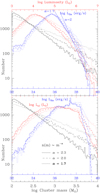 |
Fig. 7 Histogram of simulated cluster properties assuming a “stochastic” IMF. Black lines represent the cluster masses, red lines show their luminosities, and blue lines are for the Hα luminosity. The zero-age IMF is shown in the lower panel and with aging as described in the text in the upper panel. The solid, dashed, and dotted lines show the results for the different cluster mass functions (αcl = 2.3, 2.0, 1.7), following the color above. Similarly, the red x-axis provides the cluster luminosities and the blue x-axis represents the Hα luminosity, both in logarithm. In the upper panel, two blue lines are shown with slopes of 1.7 and 2.0 to help guide the eye. We drew three sets of 30 000 clusters for each of the mass functions and, after checking that they yielded the same results, they were combined to further reduce any noise so the distributions are based on 90 000 clusters for each mass function. The Chabrier IMF was used with the Eker-Sternberg MLR. |
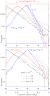 |
Fig. 8 Like Figure 7 (zero-age in lower panel, random aging up to 15 Myr in upper panel) but the maximum stellar mass is as proposed by Larson (1982) (see Sect. 5.3). One of the main differences is the lack of the broad peak near 1038erg/s. The peak is due to the presence of a massive star in a small cluster, which is no longer possible with the Larson (1982) mass limit. While the cluster mass distribution is indeed a power law, the cluster luminosity and Nion function has an α that increases slowly with the minimal luminosity used in the fit, whether the Maschberger or powerlaw.py algorithm is used. This is seen as the curvature not present in the cluster mass distribution and is the result of the limiting stellar mass. |
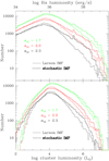 |
Fig. 9 Comparison of the distribution of cluster properties for a stochastic IMF (0.08-100 M⊙) with that derived for Larson’s model (Larson 1982) where the maximum stellar mass varies with the parent cloud mass. As in the previous figures, the cluster mass distribution is a pure power law with αcl = 1.7, 2.0, and 2.3 and Mclust = 0.03 Mcl. Cluster ages are attributed randomly as described in the text. The bolometric luminosities (bottom) and Hα luminosity (top) were then calculated for the stellar population at the age of each HII region. This figure can be directly compared with Fig. 8. |
5.3 Testing an IMF where M*,max depends on the cloud mass
We then directly tested the Larson (1982) link  by generating a mock set of cluster masses assuming that 3% of the cloud mass was converted into stars (Mclust = 0.03 × MGMC). The cluster masses range from 100 to 10 000 M⊙.
The mass functions take the values αcl = 1.7, 2.0, and 2.3. Because the smaller clouds form lower-mass massive stars, their Hα luminosity is decreased with respect to large clouds, resulting in a larger range of Hα luminosities and hence a shallower slope, very much like what is observed.
Figure 8 shows the zero-age HII region bolometric and Hα luminosity distributions, as in Fig. 7 but with the Larson (1982) M*,max. The initial slopes of the luminosity and Hα distributions are significantly shallower than the parent GMC distribution and have a slightly convex shape. However, after aging, the slopes are no longer significantly shallower than the cluster mass distribution. A comparison between the stochastic (full 0.08-100 M⊙ range) and Larson (1982) limited IMFs is shown in Fig. 9 where it is apparent that the Larson (1982) stellar mass limit yields luminosity functions that are steeper than the stochastic IMF covering the full mass range.
The difference in slope is shown in Fig. 10, where the values for the three galaxies with both measured slopes as well as the average αCO and αHα for the remaining galaxies (excluding NGC0628, NGC3627, and M33) are plotted. The open squares represent αc and αHα from the simulations given in Table 3 using the MK fit. The powerlaw.py fit (also provided in Table 3), for the same minimum value, yields slopes about 2% steeper. These simulations take aging into account (upper panels of Figures 7 and 8).
When αcl = 2 (our canonical case corresponding to the average of the PHANGS+M33 sample), the difference in slopes αcl-αHα is about 0.2 for the Larson mass limit and 0.4 for the stochastic star formation (see Table 3). The latter value (stochastic) is closer to the observed values in Figure 10.
Two options have been examined here: the stochastic and the Larson (1982) maximum stellar mass. However, Weidner & Kroupa (2006) also proposed a limiting mass for low-mass clusters and Larson (2003) presented a somewhat modified version of his 1982 proposal. In Fig. 11, the maximum stellar masses predicted by the various theories are compared as in Fig. 1 of Weidner & Kroupa (2006) except that the values have been recalculated for an IMF going from 0.08 M⊙ to 100 M⊙ using a Chabrier IMF (very similar to the Kroupa IMF: see Fig. 1) in order to make them comparable to our study. The other stellar mass limits proposed give more discrepant results from stochastic sampling than the Larson (1982) maximum mass, and hence cannot improve the agreement of the simulated distributions with the observed spectral indices in Fig. 10.
Intuitively, a stellar mass limit below the top of the IMF results in more low-luminosity HII regions, resulting in a steeper slope when fit with a power law. The lower the limit, the stronger the steepening.
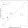 |
Fig. 10 Comparison of the observed GMC spectral index and HII region Hα luminosity spectral index with the simulations using the stochastic and Larson (1982) limited IMFs. The point marked “ave” represents the average of the galaxies observed in Hα but not in CO plotted with the average of the galaxies observed in CO but not Hα. |
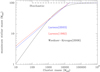 |
Fig. 11 Comparison of the Larson (1982), Larson (2003), and Kroupa-Weidner (Weidner & Kroupa 2004, 2006) maximum stellar masses as in Weidner & Kroupa (2006) Fig. 1 but recalculated for the range in stellar masses used here (0.08-100 M⊙) and a Chabrier IMF. The dashed line at 100 M⊙ gives the “stochastic” mass limit. |
6 Conclusions
The large high-quality samples of HII regions and molecular clouds now available have been used to look for systematic radial variations of the luminosity function and constraints on the IMF of stars. Only galaxies with large numbers of HII regions and/or molecular clouds were treated here to ensure statistical robustness.
The CO luminosity function always steepens with galac-tocentric distance, while the Hα luminosity function usually steepens with galactocentric distance. As the intersection of the two samples is quite small (three galaxies), it is difficult to assert that there is a true difference in behavior. However, the molecular cloud mass distribution is consistently steeper than that of the HII region Hα luminosity distribution and this may provide information on the IMF.
The main IMFs proposed in the literature (Salpeter 1955; Kroupa 2001; Chabrier 2003) differ in the low-mass end and hence only affect luminosities marginally due to the lesser mass stored in low-mass stars in the Chabrier and Kroupa IMFs as compared to Salpeter. Therefore the flatter HII region luminosity distribution cannot be due to a change in the low-mass IMF. Metallicity differences may also affect the IMF but within this sample the metallicity variation is small. It has also been proposed that massive clouds are required to be able to form the highest-mass stars. Larson (1982, 2003) suggested a maximum stellar mass of  . In this work, we compare a fully stochastically sampled IMF with the same IMF with a mass truncation as proposed in Larson (1982) or Zhou et al. (2025). Allowing for aging is essential as the highest mass stars are short-lived.
Contrary to our initial expectations, the difference between the HII region Hα luminosity function and the GMC mass function is consistent with the fully stochastically sampled IMF with no link between M*,max and GMC mass. This is in agreement with results obtained using Hα emission to trace the IMF in young stellar clusters (e.g. Corbelli et al. 2009; Jung et al. 2023). The observed scatter in the spectral indices with respect to the mean values for a stochastically sampled IMF may indicate additional dependencies on massive star formation such as chemical composition and environment (Dib 2023). More catalogs of HII regions and GMCs should become available in the near future to extend the work presented here.
References
- Alstott, J., Bullmore, E., & Plenz, D. 2014, PLoS ONE, 9, e85777 [CrossRef] [Google Scholar]
- Braine, J., Rosolowsky, E., Gratier, P., Corbelli, E., & Schuster, K.-F. 2018, A&A, 612, A51 [NASA ADS] [CrossRef] [EDP Sciences] [Google Scholar]
- Calzetti, D., Liu, G., & Koda, J. 2012, ApJ, 752, 98 [NASA ADS] [CrossRef] [Google Scholar]
- Chabrier, G. 2003, PASP, 115, 763 [Google Scholar]
- Chevance, M., Kruijssen, J. M. D., Hygate, A. P. S., et al. 2020, MNRAS, 493, 2872 [NASA ADS] [CrossRef] [Google Scholar]
- Colombo, D., Hughes, A., Schinnerer, E., et al. 2014, ApJ, 784, 3 [NASA ADS] [CrossRef] [Google Scholar]
- Corbelli, E., Verley, S., Elmegreen, B. G., & Giovanardi, C. 2009, A&A, 495, 479 [NASA ADS] [CrossRef] [EDP Sciences] [Google Scholar]
- Corbelli, E., Braine, J., Bandiera, R., et al. 2017, A&A, 601, A146 [NASA ADS] [CrossRef] [EDP Sciences] [Google Scholar]
- da Silva, R. L., Fumagalli, M., & Krumholz, M. R. 2014, MNRAS, 444, 3275 [Google Scholar]
- Demachi, F., Fukui, Y., Yamada, R. I., et al. 2024, PASJ, 76, 1059 [Google Scholar]
- Dib, S. 2023, ApJ, 959, 88 [NASA ADS] [CrossRef] [Google Scholar]
- Dickman, R. L., Snell, R. L., & Schloerb, F. P. 1986, ApJ, 309, 326 [NASA ADS] [CrossRef] [Google Scholar]
- Druard, C., Braine, J., Schuster, K. F., et al. 2014, A&A, 567, A118 [NASA ADS] [CrossRef] [EDP Sciences] [Google Scholar]
- Eker, Z., Bakιş V., Bilir, S., et al. 2018, MNRAS, 479, 5491 [NASA ADS] [CrossRef] [Google Scholar]
- Eker, Z., Soydugan, F., Soydugan, E., et al. 2015, AJ, 149, 131 [Google Scholar]
- Evans, Neal J. I., Dunham, M. M., Jørgensen, J. K., et al. 2009, ApJD, 181, 321 [Google Scholar]
- Gratier, P., Braine, J., Rodriguez-Fernandez, N. J., et al. 2012, A&A, 542, A108 [NASA ADS] [CrossRef] [EDP Sciences] [Google Scholar]
- Hopkins, A. M. 2018, PASA, 35, e039 [NASA ADS] [CrossRef] [Google Scholar]
- Jung, D. E., Calzetti, D., Messa, M., et al. 2023, ApJ, 954, 136 [Google Scholar]
- Kobayashi, M. I. N., Inutsuka, S.-i., Kobayashi, H., & Hasegawa, K. 2017, ApJ, 836, 175 [NASA ADS] [CrossRef] [Google Scholar]
- Kroupa, P. 2001, MNRAS, 322, 231 [NASA ADS] [CrossRef] [Google Scholar]
- Larson, R. B. 1982, MNRAS, 200, 159 [NASA ADS] [Google Scholar]
- Larson, R. B. 1998, MNRAS, 301, 569 [NASA ADS] [CrossRef] [Google Scholar]
- Larson, R. B. 2003, in Astronomical Society of the Pacific Conference Series, 287, Galactic Star Formation Across the Stellar Mass Spectrum, eds. J. M. De Buizer, & N. S. van der Bliek, 65 [Google Scholar]
- Leroy, A. K., Walter, F., Sandstrom, K., et al. 2013, AJ, 146, 19 [Google Scholar]
- Leroy, A. K., Schinnerer, E., Hughes, A., et al. 2021, ApJS, 257, 43 [NASA ADS] [CrossRef] [Google Scholar]
- Leroy, A. K., Sun, J., Meidt, S., et al. 2025, ApJ, 985, 14 [Google Scholar]
- Lin, Z., Hu, N., Kong, X., et al. 2017, ApJ, 842, 97 [NASA ADS] [CrossRef] [Google Scholar]
- Maschberger, T., & Kroupa, P. 2009, MNRAS, 395, 931 [NASA ADS] [CrossRef] [Google Scholar]
- Murgia, M., Crapsi, A., Moscadelli, L., & Gregorini, L. 2002, A&A, 385, 412 [NASA ADS] [CrossRef] [EDP Sciences] [Google Scholar]
- Murray, N. 2011, ApJ, 729, 133 [NASA ADS] [CrossRef] [Google Scholar]
- Rosolowsky, E. 2005, PASP, 117, 1403 [NASA ADS] [CrossRef] [Google Scholar]
- Rosolowsky, E., Keto, E., Matsushita, S., & Willner, S. P. 2007, ApJ, 661, 830 [NASA ADS] [CrossRef] [Google Scholar]
- Rosolowsky, E., Hughes, A., Leroy, A. K., et al. 2021, MNRAS, 502, 1218 [NASA ADS] [CrossRef] [Google Scholar]
- Salpeter, E. E. 1955, ApJ, 121, 161 [Google Scholar]
- Santoro, F., Kreckel, K., Belfiore, F., et al. 2022, A&A, 658, A188 [NASA ADS] [CrossRef] [EDP Sciences] [Google Scholar]
- Schinnerer, E., Hughes, A., Leroy, A., et al. 2019, ApJ, 887, 49 [NASA ADS] [CrossRef] [Google Scholar]
- Schinnerer, E., & Leroy, A. K. 2024, ARA&A, 62, 369 [Google Scholar]
- Solomon, P. M., Rivolo, A. R., Barrett, J., & Yahil, A. 1987, ApJ, 319, 730 [Google Scholar]
- Sternberg, A., Hoffmann, T. L., & Pauldrach, A. W. A. 2003, ApJ, 599, 1333 [NASA ADS] [CrossRef] [Google Scholar]
- Teng, Y.-H., Chiang, I.-D., Sandstrom, K. M., et al. 2024, ApJ, 961, 42 [NASA ADS] [CrossRef] [Google Scholar]
- Weidner, C., & Kroupa, P. 2004, MNRAS, 348, 187 [NASA ADS] [CrossRef] [Google Scholar]
- Weidner, C., & Kroupa, P. 2006, MNRAS, 365, 1333 [Google Scholar]
- Zhou, J. W., Kroupa, P., & Dib, S. 2025, MNRAS, 541, 1276 [Google Scholar]
Appendix A Further characterization of the IMF and stellar properties
The figures in this section illustrate stellar and star cluster properties. While our baseline is a Chabrier IMF from 0.08-100M⊙ and the Eker-Sternberg Mass-Luminosity relation (MLR), the figures show the differences. Fig. A.1 shows how the luminosity, radius, effective temperature, and number of ionizing photons vary with mass for the different MLRs and a Chabrier IMF from 0.08 to 100 M⊙.
Fig. A.2 shows 1000 simulated clusters, each with 300M⊙ of stars, to illustrate the importance of the most massive star in a cluster and how that varies when randomly sampling the IMF. The top panel shows the distribution of stellar masses for the 3 IMFs examined and how the median mass of the most massive star varies. The lower panel shows the total cluster luminosity for the 3 IMFs as a function of the most massive star in the cluster (Mcluster = 300M⊙) and the solid curve shows the luminosity of that star. It is apparent that the most massive star generates the majority of the cluster luminosity in most cases when its mass is M*,max > 15M⊙.
Fig. A.3 shows how clusters age as a function of time and choice of IMF. The top panel shows the average cluster mass fraction remaining as a function of time and (right hand scale) the stellar lifetime, shown as the mass of the most massive star in a cluster as a function of time. The lower panel displays how the mean light-to-mass ratio of a cluster varies with time and how the number of ionizing photons (right hand scale) decreases with cluster age.
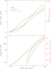 |
Fig. A.1 Mass-luminosity relation used in this work. The black line is the simple L = M3 relation, red is the generalized Eker et al. (2015), and green the Eker et al. (2018) and Sternberg et al. (2003) MLR. The dashed lines show the property on the right-hand y-axis (Temperature and number of ionizing photons). |
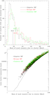 |
Fig. A.2 The top panel shows the distribution of the masses of the most massive star in each cluster, with the median value indicated, for the 1000 simulated clusters of 300M⊙ each. These median values are close to the maximal value suggested by Larson (1982). Even for a cluster with 300M⊙ of stars, the random sampling effect is huge. The bottom panel shows the total cluster luminosity as a function of the mass of the most massive star, for the three IMFs indicated by their color. The line shows the luminosity of the single most massive star in the cluster. We can see (1) that the luminosity of a 300M⊙ cluster can vary by a factor 1000 and (2) how important the most massive star is for the total zero-age luminosity as when a very massive star is present, it dominates the luminosity (and ionizing photon production) of the cluster for its lifetime. |
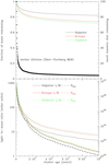 |
Fig. A.3 Time evolution of the stellar population in a cluster. The black line shows the Salpeter IMF, red for Kroupa, and the green line is for the Chabrier IMF. The black triangles and dashed lines show the property on the right-hand y-axis (maximum stellar mass and number of ionizing photons per M⊙). |
All Tables
All Figures
|
Fig. 1 Initial mass functions used in this work. Black line is for Salpeter, red is for Kroupa, and green is for the Chabrier IMF. The plot shows the number of stars per logarithmic mass interval for each mass. Clearly, the Kroupa and Chabrier IMFs are similar and have significantly fewer low-mass stars than the Salpeter IMF. The dashed and dotted lines show the Kroupa IMF using somewhat higher characteristic masses. The effect of increasing the characteristic mass is that there are fewer low mass stars so the L/M ratio of the stellar population increases from about 900 L⊙/M⊙ to 1500 L⊙/M⊙. |
| In the text | |
|
Fig. 2 Link between spectral index measured with powerlaw.py and Lmin for the 19 galaxies from data given in Table 2 of Santoro et al. (2022). Lmin is normalized by the completeness limit Lcompl to be comparable from one galaxy to another. |
| In the text | |
|
Fig. 3 Probability density functions of Hα fluxes from NGC0628, NGC3627, and M 33, the three galaxies for which both HII region and GMC catalogs are available. Results of the powerlaw.py (red line) and Maschberger & Kroupa (2009) (blue line) fits along with observational data for NGC0628, NGC3627, and M33 from Santoro et al. (2022) and Lin et al. (2017) are shown. NGC0628 and NGC3627 are the two PHANGS galaxies for which both the HII region and GMC samples are available. The Hα data for M33 are from Lin et al. (2017). The adopted completeness limit for the fits (equivalent of Lmin in Santoro et al. 2022) are shown as a dashed green line and given in Table 1 The error bars are proportional to |
| In the text | |
|
Fig. 4 Probability density functions of CO luminosities from NGC0628, NGC3627m and M33, the three galaxies for which both HII region and GMC catalogs are available. Results of powerlaw.py (red line) and Maschberger & Kroupa (2009) fit (blue line) along with observational data for NGC0628, NGC3627, and M33 from Rosolowsky et al. (2021) and Corbelli et al. (2017). NGC0628 and NGC3627 are the two PHANGS galaxies for which both the H II region and GMC samples are available. The CO data for M33 are from Druard et al. (2014) and Corbelli et al. (2017). The adopted completeness limits for the fits are the first of the limits given in Table 5 of Rosolowsky et al. (2021) and are shown as a dashed green line and given in Table 2. The error bars are proportional to |
| In the text | |
|
Fig. 5 Results of fits to the distribution of Hα and CO luminosities. For each galaxy, the name is indicated followed by (1) the whole-galaxy GMC spectral index; (2) the whole-galaxy Hα spectral index; (3) the inner and outer GMC spectral index, connected by a line; and (4) the same but or the Hα luminosities of HII regions. In each case, the triangles indicate the values obtained from the two independent fitting methods and the average is shown by the short horizontal line. When the line goes up, the distribution in the outer part is steeper (relatively more small objects). A horizontal dashed line at a value of 1.5 is plotted to allow easy appraisal of the values. |
| In the text | |
|
Fig. 6 Radial variation of spectral indices. This plot portrays the latter four columns of Fig. 5 in a simpler fashion. The lines start with the median position of the inner regions (H II or GMC) and end at the median position of the outer regions. The marker near the line center indicates the median galactocentric distance of the whole sample, and column 5 of Tables 1 and 2 provides the correspondence with the optical radius R25. Red lines are GMC indices and black lines show the indices of the HII regions. When the line goes up, the spectral index in the outer part is higher because the distribution is steeper (relatively more small objects). |
| In the text | |
|
Fig. 7 Histogram of simulated cluster properties assuming a “stochastic” IMF. Black lines represent the cluster masses, red lines show their luminosities, and blue lines are for the Hα luminosity. The zero-age IMF is shown in the lower panel and with aging as described in the text in the upper panel. The solid, dashed, and dotted lines show the results for the different cluster mass functions (αcl = 2.3, 2.0, 1.7), following the color above. Similarly, the red x-axis provides the cluster luminosities and the blue x-axis represents the Hα luminosity, both in logarithm. In the upper panel, two blue lines are shown with slopes of 1.7 and 2.0 to help guide the eye. We drew three sets of 30 000 clusters for each of the mass functions and, after checking that they yielded the same results, they were combined to further reduce any noise so the distributions are based on 90 000 clusters for each mass function. The Chabrier IMF was used with the Eker-Sternberg MLR. |
| In the text | |
|
Fig. 8 Like Figure 7 (zero-age in lower panel, random aging up to 15 Myr in upper panel) but the maximum stellar mass is as proposed by Larson (1982) (see Sect. 5.3). One of the main differences is the lack of the broad peak near 1038erg/s. The peak is due to the presence of a massive star in a small cluster, which is no longer possible with the Larson (1982) mass limit. While the cluster mass distribution is indeed a power law, the cluster luminosity and Nion function has an α that increases slowly with the minimal luminosity used in the fit, whether the Maschberger or powerlaw.py algorithm is used. This is seen as the curvature not present in the cluster mass distribution and is the result of the limiting stellar mass. |
| In the text | |
|
Fig. 9 Comparison of the distribution of cluster properties for a stochastic IMF (0.08-100 M⊙) with that derived for Larson’s model (Larson 1982) where the maximum stellar mass varies with the parent cloud mass. As in the previous figures, the cluster mass distribution is a pure power law with αcl = 1.7, 2.0, and 2.3 and Mclust = 0.03 Mcl. Cluster ages are attributed randomly as described in the text. The bolometric luminosities (bottom) and Hα luminosity (top) were then calculated for the stellar population at the age of each HII region. This figure can be directly compared with Fig. 8. |
| In the text | |
|
Fig. 10 Comparison of the observed GMC spectral index and HII region Hα luminosity spectral index with the simulations using the stochastic and Larson (1982) limited IMFs. The point marked “ave” represents the average of the galaxies observed in Hα but not in CO plotted with the average of the galaxies observed in CO but not Hα. |
| In the text | |
|
Fig. 11 Comparison of the Larson (1982), Larson (2003), and Kroupa-Weidner (Weidner & Kroupa 2004, 2006) maximum stellar masses as in Weidner & Kroupa (2006) Fig. 1 but recalculated for the range in stellar masses used here (0.08-100 M⊙) and a Chabrier IMF. The dashed line at 100 M⊙ gives the “stochastic” mass limit. |
| In the text | |
|
Fig. A.1 Mass-luminosity relation used in this work. The black line is the simple L = M3 relation, red is the generalized Eker et al. (2015), and green the Eker et al. (2018) and Sternberg et al. (2003) MLR. The dashed lines show the property on the right-hand y-axis (Temperature and number of ionizing photons). |
| In the text | |
|
Fig. A.2 The top panel shows the distribution of the masses of the most massive star in each cluster, with the median value indicated, for the 1000 simulated clusters of 300M⊙ each. These median values are close to the maximal value suggested by Larson (1982). Even for a cluster with 300M⊙ of stars, the random sampling effect is huge. The bottom panel shows the total cluster luminosity as a function of the mass of the most massive star, for the three IMFs indicated by their color. The line shows the luminosity of the single most massive star in the cluster. We can see (1) that the luminosity of a 300M⊙ cluster can vary by a factor 1000 and (2) how important the most massive star is for the total zero-age luminosity as when a very massive star is present, it dominates the luminosity (and ionizing photon production) of the cluster for its lifetime. |
| In the text | |
|
Fig. A.3 Time evolution of the stellar population in a cluster. The black line shows the Salpeter IMF, red for Kroupa, and the green line is for the Chabrier IMF. The black triangles and dashed lines show the property on the right-hand y-axis (maximum stellar mass and number of ionizing photons per M⊙). |
| In the text | |
Current usage metrics show cumulative count of Article Views (full-text article views including HTML views, PDF and ePub downloads, according to the available data) and Abstracts Views on Vision4Press platform.
Data correspond to usage on the plateform after 2015. The current usage metrics is available 48-96 hours after online publication and is updated daily on week days.
Initial download of the metrics may take a while.