| Issue |
A&A
Volume 697, May 2025
|
|
|---|---|---|
| Article Number | A81 | |
| Number of page(s) | 15 | |
| Section | Extragalactic astronomy | |
| DOI | https://doi.org/10.1051/0004-6361/202453331 | |
| Published online | 07 May 2025 | |
SEMPER
I. A novel semi-empirical model for the radio emission of star-forming galaxies at 0 < z < 5
1
INAF – Istituto di Radioastronomia, Via Gobetti 101, 40129 Bologna, Italy
2
Scuola Internazionale Superiore di Studi Avanzati, Via Bonomea 265, 34136 Trieste, Italy
3
Dipartimento di Fisica e Astronomia “G. Galilei”, Università di Padova, Via Marzolo 8, 35131 Padova, Italy
4
INAF – Istituto di Radioastronomia – Italian ALMA Regional Centre, Via Gobetti 101, 40129 Bologna, Italy
5
IFPU – Institute for Fundamental Physics of the Universe, Via Beirut 2, 34014 Trieste, Italy
6
INFN-Sezione di Trieste, Via Valerio 2, 34127 Trieste, Italy
7
Dipartimento di Fisica e Astronomia “G. Galilei”, Università di Padova, Via Marzolo 8, 35131 Padova, Italy
8
INAF, Osservatorio Astronomico di Padova, Vicolo dell’Osservatorio 5, 35122 Padova, Italy
9
Universität Heidelberg, Zentrum für Astronomie, Institut für Theoretische Astrophysik, Albert-Ueberle-Str. 3, 69120 Heidelberg, Germany
10
Leiden Observatory, Leiden University, PO Box 9513 NL-2300 RA Leiden, The Netherlands
⋆ Corresponding author: m.giulietti@ira.inaf.it
Received:
6
December
2024
Accepted:
24
March
2025
Context. Star-forming galaxies (SFGs) are the dominant population in the faint radio sky, corresponding to flux densities at 1.4 GHz < 0.1 mJy. A panchromatic approach is essential for selecting SFGs in the radio band and understanding star formation processes over cosmic time. Semi-empirical models are valuable tools to effectively study galaxy formation and evolution, relying on minimal assumptions and exploiting empirical relations between galaxy properties and enabling us to take full advantage of the recent progress in radio and optical/near-infrared (NIR) observations.
Aims. In this paper, we develop the Semi-EMPirical model for Extragalactic Radio emission (SEMPER) to predict radio luminosity functions and number counts at 1.4 GHz and 150 MHz for SFGs. SEMPER is based on state-of-the-art empirical relations, with the goal of better understanding the radio properties of high-z, massive galaxy populations.
Methods. We combine the redshift-dependent galaxy stellar mass functions obtained from the recent COSMOS2020 catalogue, which exploits deep NIR observations, with up-to-date observed scaling relations such as the galaxy main sequence and the mass-dependent far-infrared/radio correlation across cosmic time. Our luminosity functions are compared with recent observational determinations from the Very Large Array (JVLA), the Low-Frequency Array (LOFAR), the Westerbork Synthesis Radio Telescope (WSRT), the Giant Metrewave Radio Telescope (GMRT) and the Australian Telescope Compact Array (ATCA), along with previous semi-empirical models and simulations.
Results. Our semi-empirical model successfully reproduces the observed luminosity functions at 1.4 GHz and 150 MHz up to z ∼ 5 and the most recent number count statistics from radio observations in the LOFAR Two-metre Sky Survey (LoTSS) deep fields. Our model, based on galaxies selected in the NIR, naturally predicts the presence of radio-selected massive and/or dust-obscured galaxies already in place at high redshift (z ≳ 3.5), as suggested by recent results from the James Webb Space Telescope (JWST). Our predictions offer an excellent benchmark for upcoming updates from JWST and future ultra-deep radio surveys planned with the Square Kilometre Array (SKA) and its precursors.
Key words: galaxies: luminosity function / mass function / radio continuum: galaxies
© The Authors 2025
 Open Access article, published by EDP Sciences, under the terms of the Creative Commons Attribution License (https://creativecommons.org/licenses/by/4.0), which permits unrestricted use, distribution, and reproduction in any medium, provided the original work is properly cited.
This article is published in open access under the Subscribe to Open model. Subscribe to A&A to support open access publication.
1. Introduction
Star-forming galaxies (SFGs) emit in the radio band due to synchrotron radiation originating from electrons accelerated in supernova remnants and free-free continuum emission from hot and ionised HII regions. The radio luminosity, therefore, constitutes an effective tracer of the star-formation rate (SFR) of galaxies (Condon et al. 2002; Kennicutt & Evans 2012) provided that the contribution of the active galactic nuclei (AGN) is negligible. The link between radio emission and SFR can be derived from the tight correlation observed between the radio and far-infrared (FIR) luminosities (Helou et al. 1985; Condon 1992; Lacki & Thompson 2010; Murphy et al. 2011), with the latter tracing the star formation activity in dust-enshrouded environments. With respect to other tracers, such as the ultraviolet (UV) and Hα luminosities, the radio emission is unaffected by dust extinction and can be efficiently exploited to study the dust-obscured star-formation (e.g. Chapman et al. 2004).
Radio astronomy has been transformed by the increasing capability to detect SFGs which dominate the faint radio sky, gradually emerging from radio-loud (RL) AGNs at sub-mJy flux level and becoming increasingly prominent at flux densities below ∼100 μJy at 1.4 GHz (Smolčić et al. 2008, 2017; Padovani et al. 2015; Padovani 2016; Prandoni et al. 2018; Algera et al. 2020; van der Vlugt et al. 2021). The faint radio populations also include a significant fraction of radio quiet (RQ) AGNs, which exhibit evidence of nuclear activity in the X-ray, mid-IR, or optical bands but show weak radio emission (i.e. no large-scale jets). The origin of the radio emission in these objects remains a topic of debate, primarily due to the difficulty in disentangling the contribution of the central nucleus from that of the host galaxy (Bonato et al. 2017; Mancuso et al. 2017; Ceraj et al. 2018; Prandoni et al. 2018). Understanding these faint radio populations has been possible thanks to the significantly improved sensitivity of current deep and wide radio surveys (e.g. Helfand et al. 2015; Lacy et al. 2020; Norris et al. 2021; Heywood et al. 2022; Shimwell et al. 2022), which have opened up new opportunities for studying the radio sky. These surveys are playing an increasingly important role in the field of galaxy evolution, providing a new avenue for investigating the star formation history of galaxies up to high redshifts (see reviews by de Zotti et al. 2010; Padovani 2016; Mancuso et al. 2015; Duchesne et al. 2024; Bonato et al. 2021a; Giulietti et al., in prep.). This has become possible thanks to the upgraded sensitivity of radio telescopes such as the Karl G. Jansky Very Large Array (JVLA) and the advent of new-generation radio telescopes such as MeerKAT (Jarvis et al. 2016), the Low-Frequency Array (LOFAR, van Haarlem et al. 2013) and the Australian Square Kilometre Array Pathfinder (ASKAP, Johnston et al. 2007) and with the forthcoming Square Kilometre Array (SKA).
A panchromatic approach is indispensable in selecting SFGs in the radio band, for this reason, deep radio surveys have been conducted in sky fields covered by a wealth of multi-wavelength (X-ray to radio) data (e.g. Jarvis et al. 2016; Novak et al. 2017; Smolčić et al. 2017; Prandoni et al. 2018; Bonato et al. 2021a,b; Duncan et al. 2021; Kondapally et al. 2021; Sabater et al. 2021; Tasse et al. 2021;Heywood et al. 2022; Whittam et al. 2022; Best et al. 2023).
Recent advancements in radio observations of these sky regions have mirrored those in the optical/near-IR bands. For instance, in the Cosmic Evolution Survey (COSMOS) field, the latest COSMOS2020 catalogue (Weaver et al. 2022, 2023) has benefited from the fourth data release of the UltraVISTA survey (McCracken et al. 2012; Moneti et al. 2023, Ks = 25.7 at 5σ), along with new observations from the James Webb Space Telescope (JWST) as part of the COSMOS-Web project (Casey et al. 2023; Shuntov et al. 2025). In the North Ecliptic Pole, the Hawaii eROSITA Ecliptic Pole Survey Catalog (HEROES, Taylor et al. 2023) has recently been published, and upcoming data from the Euclid mission (Euclid Collaboration: Scaramella et al. 2022) will provide sub-arcsec NIR imaging down to H = 26 mag.
We now require a coherent, multi-wavelength approach that weaves together these advancements, providing a comprehensive view of the processes driving star formation as a function of redshift. Motivated by this, in this work we have developed a semi-empirical model which leverages recent estimates of the evolution of galaxies stellar mass function (SMF), based on the NIR data from the COSMOS2020 catalogue (Weaver et al. 2022, 2023), with the main goal of predicting the statistics of SFGs in the radio band.
Semi-empirical models have recently been proven to be an effective approach to galaxy formation and evolution (e.g. Behroozi et al. 2013, 2019; Moster et al. 2013, 2018; Mancuso et al. 2016a; Grylls et al. 2019; Bisigello et al. 2022; Fu et al. 2022; Boco et al. 2023; see also the review by Lapi et al. 2025). At variance with cosmological hydrodynamic simulations (see Vogelsberger et al. 2020 for a review) and semi-analytic models (e.g. Lacey et al. 2016; Lagos et al. 2018; Henriques et al. 2020; Parente et al. 2023), semi-empirical models do not aim to describe the small-scale physics governing the baryon cycle from first principles. Instead, they rely on empirical relations between spatially averaged galaxy properties, keeping the number of parameters and assumptions to a minimum. The main limitation of this approach is that, being inherently data-driven, it is less suitable for uncovering the details behind the physical processes involved. However, given their small number of parameters, semi-empirical models are easily expandable and computationally efficient. At the same time, they can also be exploited to identify inconsistencies between datasets by connecting different observables and efficiently performing predictions for future missions.
In this paper, we leverage state-of-the-art scaling relations to develop the up-to-date Semi-EMPirical model for Extragalactic Radio emission (SEMPER), used to predict luminosity functions (LFs) and number count statistics of SFGs in the radio band. In particular, we combine the redshift-dependent galaxy SMF of Weaver et al. (2023, W23 hereafter) and various observed relations, such as the galaxy main sequence (MS; Brinchmann et al. 2004; Noeske et al. 2007) and the recently derived mass- and redshift- dependent far-infrared/radio correlation (FIRRC, Delvecchio et al. 2021; McCheyne et al. 2022). Our predictions are compared with state-of-the-art continuum observations at 1.4 GHz and 150 MHz from deep radio surveys conducted with the JVLA, LOFAR, the Westerbork Synthesis Radio Telescope (WSRT), the Giant Metrewave Radio Telescope (GMRT) and the Australian Telescope Compact Array (ATCA), along with the recent Tiered Radio Extragalactic Continuum Simulation (T-RECS, Bonaldi et al. 2019, 2023) and previous semi-empirical models (Mancuso et al. 2017) for SFGs emitting in the radio-band. To extend our comparison analysis we also derive the 150 MHz radio number counts derived from the recent LOFAR Two-metre Sky Survey (LoTSS; Shimwell et al. 2017, 2019, 2022) three deep fields (Duncan et al. 2021; Kondapally et al. 2021; Sabater et al. 2021; Tasse et al. 2021; Best et al. 2023; Cochrane et al. 2023). This is the first of a series of papers; in a forthcoming work, we will expand SEMPER to include radio emission from AGNs.
The paper is structured as follows. Sect. 2, we describe our model and its main ingredients, Sect. 3, we describe the datasets exploited in this work as a comparison to our model. In Sect. 4, we present and discuss our results, and finally, we draw our conclusions in Sect. 5.
In this work, we assume a Chabrier (2003) initial mass function (IMF) and a standard ΛCDM cosmology with parameters: H0 = 70 km s−1 Mpc−1, ΩΛ, 0 = 0.7 and Ωm, 0 = 0.3, such that h70 ≡ H0/(70 km s−1 Mpc−1) = 1. All magnitudes are expressed in the AB system (Oke 1974). The radio source spectra are assumed to be described by a simple power law Sν ∝ να, where Sν is the monochromatic flux density at a certain frequency ν and α is the radio spectral index.
2. Method
In this section, we describe the key ingredients of our semi-empirical model.
2.1. Stellar mass functions
We exploited the recent SMFs for SFGs reported by W23, expressed as N(z, log M⋆) and based on the most recent data release of the COSMOS2020 catalogue (Weaver et al. 2022). This choice is motivated by two main reasons. First, COSMOS is one of the deepest and most studied fields, benefitting from a broad UV-to-radio coverage. The izYJHKs coadded image of COSMOS2020 reaches magnitudes down to 26 AB and ensures completeness down to 109 M⊙ at z ≈ 3 for a mass-selected sample of ∼1 000 000 galaxies. Second, the objects’ classifications, photometric redshifts, and physical properties are robustly supported by extensive photometry, spanning from UV to 8 μm across a total area of 2 deg2 (see Weaver et al. 2022 and W23 for details).
From the COSMOS2020 photo-z catalogue, W23 retrieved the galaxies SMF’s shape and evolution from z ≈ 0.2 up to z = 7.5 for the total mass-complete sample and up to z = 5.5 for the quiescent and star-forming mass-complete sub-samples. We exploited the observed measurements and the maximum likelihood parameters found by W23 (see their Table C.2.) from their Monte Carlo Markov Chain (MCMC) analysis to retrieve the best-fit curves for SFGs, described by a double (single) Schechter function for galaxies at z < 3 (z > 3):
![$$ \begin{aligned} \begin{aligned} \Phi \mathrm{d}\log M =&\ln (10) e^{-10^{\log M-\log M^*}}\\&\times \left[\Phi _1^*\left(10^{\log M-\log M^*}\right)^{\alpha _1+1}\right.\\&\left.+\Phi _2^*\left(10^{\log M-\log M^*}\right)^{\alpha _2+1}\right] \mathrm{d}\log M. \end{aligned} \end{aligned} $$](/articles/aa/full_html/2025/05/aa53331-24/aa53331-24-eq1.gif)
In this equation, Φ1* and Φ2* are the individual normalisation of the two functions, α1 and α2 the relative low-mass slopes and M* the characteristic stellar mass.
One of the main findings of W23 is the high number density of massive galaxies (M⋆ > 1011 M⊙) between 3 < z ≤ 5.5 compared to previous analyses using an identical selection (Davidzon et al. 2017). These massive SFGs have extreme red colours and are ≳1 order of magnitude fainter than the median Ks AB magnitude of the sample. Most of these galaxies (> 60%) were classified as star-forming systems at z > 1, a fraction of which is likely to be dust-obscured and extremely faint in the NIR, being therefore missed by previous studies (see Sect. 4.2). Because the Schechter formalism employed in W23 to fit the observed SMFs fails to reproduce the excess of massive and extremely red galaxies, in this study, we re-fitted the observed SMFs from W23. To do so, we employed a simple double power-law function of the form:
where logΦ1 and logΦ2 are the normalisations of the two power laws, α and β are the two slopes and log M0 represents the mass corresponding to the slope-change.
Since the SMFs presented in W23 are limited to z ≳ 0.2, we included SFGs at lower redshifts by exploiting the recent SMFs reported in the Galaxy And Mass Assembly Survey Data Release 4 (GAMA DR4; Driver et al. 2022). The GAMA survey (Driver et al. 2011) covers five sky regions for a total of 250 deg2, providing images and spectroscopic redshifts for ∼230 000 sources along with UV-to-FIR 20-band photometry. Driver et al. (2022) divided the SMF for morphological type, extending the estimates to a lower mass limit of 106.75 M at z < 0.1. In this work, we selected the SMFs of the morphological type ‘D’, corresponding to single-component late-type systems, dominating the stellar mass density for local galaxies for stellar masses M⋆ < 109.25 M
 , under the assumption that these galaxies are the primary star-forming systems in the local Universe. To model the observed measurements of galaxies at z < 0.08, Driver et al. (2022) elected a single Schechter function. In this case, we adopted Eq. (2) to maintain consistency with our approach in fitting W23’s observations.
We reconstructed the SMF’s shape via a Bayesian MCMC framework. We exploited the Python package emcee (Foreman-Mackey et al. 2013). We discuss the details of our fitting procedure in Appendix A. The results are shown in Figs. A.1 and A.2 and are compared with the best fits obtained respectively by Driver et al. (2022) and W23. Our Double Power Law fit successfully reproduces the observed data for all the redshift bins and traces the high-mass points for z > 3, where the Double Schechter profile fails. As a second step of our analysis, we built a continuity model to obtain the shape and evolution of SMFs by fitting the double power law’s parameters as a function of redshift. This approach enables a full redshift interpolation of our model, particularly in the redshift bin 0.08 < z < 0.2, where no observations are available.
2.2. Main sequence
The next step involves computing the star-formation rate function (SFRF) to determine the distribution in SFR for SFGs at a given redshift. We therefore exploit the well-known MS relation (Brinchmann et al. 2004; Noeske et al. 2007).
The MS is a tight relation linking the stellar mass and the SFR (ψ) of a galaxy over a wide range of redshifts (0 < z < 6) through the specific star-formation rate (sSFR ≡  ). This relation has been extensively studied over the past decade both observationally and theoretically (see e.g. Daddi et al. 2007, 2022; Rodighiero et al. 2011, 2015; Speagle et al. 2014; Whitaker et al. 2014; Schreiber et al. 2015; Mancuso et al. 2016b; Dunlop et al. 2017; Bisigello et al. 2018; Pantoni et al. 2019; Lapi et al. 2020; Leslie et al. 2020; Thorne et al. 2021; Leja et al. 2022; Popesso et al. 2023), even though its redshift evolution, scatter and exact shape are still debated (Peng et al. 2010; Rodighiero et al. 2014; Speagle et al. 2014; Whitaker et al. 2014; Renzini & Peng 2015; Schreiber et al. 2015; Pearson et al. 2018; Popesso et al. 2019a,b; Leslie et al. 2020; Thorne et al. 2021; Leja et al. 2022), in particular in the high-mass regime.
In our model, we used the recent results by Popesso et al. (2023), which compiles numerous literature studies converted to a common calibration, covering a wide range of redshifts and stellar masses. However, it must be noted that the MS is an average relation between the stellar mass and the SFR, and it displays some dispersion and significant outliers. Several studies suggest that SFGs, at a fixed redshift and stellar mass, are distributed in SFR following a double Gaussian shape (Béthermin et al. 2012; Sargent et al. 2012; Ilbert et al. 2015; Schreiber et al. 2015). The dominant population consists of MS galaxies, and their Gaussian distribution in SFR is centred around the MS value. In contrast, the sub-complementary population of starburst galaxies have a SFR distribution centred around a value 3 − 4σ above the MS value. Several authors (e.g. Caputi et al. 2017; Bisigello et al. 2018; Rinaldi et al. 2025) have found an increase in starburst fraction, compared to the MS, for low mass (M⋆ ≤ 109) or higher redshift (z ≥ 2 − 3) galaxies.
In this work, we are assuming the double-Gaussian decomposition proposed by Sargent et al. (2012) and also adopted in recent works (Boco et al. 2021), describing the SFR distribution of a galaxy at fixed mass and redshift as:
![$$ \begin{aligned} \frac{\mathrm{d}p}{\mathrm{d}\log \psi }\left(\psi \mid z, M_{\star }\right) =&\left(\frac{A_{\mathrm{MS} }}{\sqrt{2\pi \sigma ^2_{\rm MS}}}\right) \exp \left[-\frac{\left(\log \psi -\langle \log \psi \rangle _{\mathrm{MS} }\right)^2}{2 \sigma _{\mathrm{MS} }^2}\right]\nonumber \\&+\left(\frac{A_{\mathrm{SB} }}{\sqrt{2\pi \sigma ^2_{\rm SB}}}\right) \exp \left[-\frac{\left(\log \psi -\langle \log \psi \rangle _{\mathrm{SB} }\right)^2}{2 \sigma _{\mathrm{SB} }^2}\right]. \end{aligned} $$](/articles/aa/full_html/2025/05/aa53331-24/aa53331-24-eq6.gif)
In the above equation, the starburst fractions are fixed and do not change with redshift and mass, and the parameters AMS = 0.97 and ASB = 0.03 represent the fraction of MS and starburst galaxies, respectively. ⟨log ψ⟩MS represents the first Gaussian’s central value and refers to the MS and ⟨log ψ⟩SB = ⟨log ψ⟩MS + 0.59 is the central value of the second Gaussian referring to SB galaxies. Values are from Sargent et al. (2012). The one-sigma dispersion of the first and second Gaussian were also fixed to the values found by Sargent et al. (2012), which are σMS = 0.188 and σSB = 0.243, respectively. By convolving Eq. (3) with the SMFs, one obtains galaxies’ SFR-functions as:
2.3. Far-IR/radio correlation
We now need to express the SFR as a function of galaxies’ radio luminosity. For this purpose, we adopted the FIRRC, a tight relation linking the monochromatic non-thermal radio emission and the FIR emission of SFGs (see e.g. Helou et al. 1985; Condon 1992; Yun et al. 2001).
The FIRRC is described via the parameter qFIR (Bell 2003; Ivison et al. 2010a,b; Sargent et al. 2010), defined as:
![$$ \begin{aligned} q_{\mathrm{FIR} }=\log \left(\frac{L_{\mathrm{FIR} }[\mathrm{W}]/3.75 \times 10^{12}}{L_{\rm 1.4\,GHz}\left[\mathrm{W\,Hz}^{-1}\right]}\right), \end{aligned} $$](/articles/aa/full_html/2025/05/aa53331-24/aa53331-24-eq8.gif)
where L1.4 GHz is the rest-frame radio luminosity and LFIR is the rest-frame FIR luminosity defined in the range 8−1000 μm.
Because of the low scatter of this relation (1σ ≈ 0.26 dex), radio emission can be used as an unbiased dust-independent tracer of star formation in galaxies and as an unbiased probe of the cosmic star formation history. This is particularly promising in the context of forthcoming large-area and deep radio surveys conducted by SKA and its precursors, reaching unprecedented sensitivity and hence able to trace SFGs to very high redshift (Jarvis et al. 2015; Mancuso et al. 2015; Schleicher & Beck 2016; An et al. 2021; Cochrane et al. 2023; Ocran et al. 2023).
Although the FIRRC has been well established at low redshift (Condon 1992; Yun et al. 2001; Bell 2003; Jarvis et al. 2010; Wang et al. 2019; Molnár et al. 2021), its redshift evolution, if present, is still debated. On the one hand, some studies point towards a redshift evolution, expressed as  (0.12 ≲ β ≲ 0.2, Basu et al. 2015; Magnelli et al. 2015; Tabatabaei et al. 2016; Calistro Rivera et al. 2017; Delhaize et al. 2017; Ocran et al. 2020a; Sinha et al. 2022). On the other hand, others report no significant redshift evolution (see e.g. Sargent et al. 2010), suggesting that the observed decreasing trend may be originated by selection effects (Bourne et al. 2011; Molnár et al. 2021). These effects have been extensively studied and can be attributed to either the different relative sensitivities of radio and FIR surveys (Sargent et al. 2010; Bourne et al. 2011; Molnár et al. 2021), leading to flux-limited samples that are biased towards more massive galaxies, or to different galaxy populations dominating at different redshifts (De Zotti et al. 2024). Recently, several studies investigated the mass-dependency of the FIRRC, reporting a decrease in
  with increasing stellar mass (Gürkan et al. 2018; Delvecchio et al. 2021; Smith et al. 2021; McCheyne et al. 2022). In this work, we used the recent relation, including both the redshift and stellar mass dependence, presented in Delvecchio et al. (2021) and McCheyne et al. (2022) to retrieve the LF at 1.4 GHz and 150 MHz.
Delvecchio et al. (2021) retrieved the redshift and mass-dependent FIRRC at 1.4 GHz for a sample of > 400 000 SFGs in the COSMOS field. SFGs were identified in the redshift and mass ranges 0.1 < z < 4.0 and 108 < M⋆/M⊙ < 1012 through colour-selection [(NUV − r)/(r − J)] criteria. The IR information was obtained from the de-blended data from Jin et al. (2018), comprising Spitzer/MIPS 24 μm data (PI: D. Sanders, Le Floc’h et al. 2009) Herschel/PACS 100 and 160 μm data from the PEP (PI: D. Lutz; Lutz et al. 2011) and SPIRE 250, 350 and 500 μm of the Herschel Multi-tiered Extragalactic Survey (HerMES, PI: S. Oliver, Oliver et al. 2012). Radio images were obtained from the VLA COSMOS 3 GHz survey (Smolčić et al. 2017). Furthermore, a median stacking procedure was performed for non-detections in different M⋆ − z bins to infer the average flux densities in each band. The relation obtained by Delvecchio et al. (2021) derived at 1.4 GHz is the following:
However, it should be pointed out that, due to the relatively small area of the COSMOS survey (2 deg2), the qIR estimates at high stellar masses suffer from significant uncertainty at low-redshift (z < 0.4), resulting in a higher normalisation compared to higher-redshifts (z > 0.4). It should also be noticed that the LFIR–SFR conversion may not be fully applicable for low-mass/metallicity and less obscured systems (Mannucci et al. 2010; Pannella et al. 2015; Whitaker et al. 2017), where the contribution of UV emission can be comparable to that of FIR emission (Buat et al. 2012; Cucciati et al. 2012; Burgarella et al. 2013). For this reason, Delvecchio et al. (2021) introduced a different formalism, which takes into account the contribution of dust-uncorrected UV emission through the parameter qSFRUV + FIR. The redshift- and mass-dependent relation is given as:
In this paper, we adopted this latter relation as it better accounts for galaxies’ total SFR by also including UV emission. When referring to the FIRRC of Delvecchio et al. (2021), we specifically mean the one defined in Eq. (7), even though it includes the contribution of the UV luminosity.
The FIRRC at low frequencies (150 MHz) has been less explored. Nevertheless, the mass-dependence and redshift evolution was investigated by Calistro Rivera et al. (2017), Read et al. (2018) and Gürkan et al. (2018) and recently extended up to z ∼ 1 by Smith et al. (2021) and McCheyne et al. (2022). McCheyne et al. (2022) derived the FIRRC in the context of the LoTSS (Sabater et al. 2021, see also Sect. 4.4) utilising LOFAR 150 MHz observations of a mass-complete sample in the ELAIS-N1 field (Kondapally et al. 2021; Duncan et al. 2021), combined with deblended Herschel data (Vaccari 2015; Hurley et al. 2017). Their FIRRC, derived at 150 MHz, is expressed as:
The LOFAR observations exploited by McCheyne et al. (2022) have similar depth to the VLA COSMOS 3 GHz survey but cover an area three times larger. This allowed the authors to probe the rare high FIR and radio luminosity populations, likely absent in smaller fields. Two samples were considered, one comprising sources with z < 1.0 and M⋆ > 1010.45 M⊙, the other including objects at z < 0.4 and M⋆ > 1010.05 M⊙. In both cases, the probed stellar masses reach up to a value of M⋆ ∼ 1011.4 M⊙. With respect to Delvecchio et al. (2021), McCheyne et al. (2022) FIRRC spans a lower redshift range (z < 1) and is found to have a different normalisation, as well as a steeper dependence on M⋆. The origin of this discrepancy is still unclear. The authors argued that it may result from either different ratios of thermal to synchrotron emission at the respective frequencies or the choice of the spectral index used to convert fluxes from 1.4 GHz and 150 MHz and vice-versa. Indeed, McCheyne et al. (2022) have shown that the difference between the two relations becomes negligible when adopting the value α = −0.59, which is slightly shallower than the typical value assumed for SFGs (α = −0.7; see e.g. Novak et al. 2017).
2.4. Inferring the radio luminosity function
We expressed Eq. (4) in terms of Lν by exploiting the mass- and redshift-dependent FIRRC. For this purpose, we convolved the resulting expression with a Gaussian distribution representing the probability of a given Lν at fixed ψ, M⋆ and z:
![$$ \begin{aligned} \begin{aligned} \frac{\mathrm{d}p}{\mathrm{d}\log {L_{\nu }}} \left(\log L_{\nu } \mid \psi , M_{\star },z \right) =&\left(\frac{1}{\sqrt{2\pi \sigma ^2_{\rm FIRRC}}}\right) \\&\times \exp \left[-\frac{\left(\log L_{\nu } - \langle \log L_{\nu } \rangle \right)^2}{2 \sigma ^2_{\rm FIRRC}}\right]. \end{aligned} \end{aligned} $$](/articles/aa/full_html/2025/05/aa53331-24/aa53331-24-eq14.gif)
The term σFIRRC accounts for the scatter of the FIRRC. ⟨log Lν⟩ is the radio luminosity at a frequency ν corresponding to a given ψ, obtained from the mean FIRRC adopting LFIR = kFIRψ (Kennicutt & Evans 2012) with kFIR being a calibration constant rescaled for a Chabrier IMF. The final expression for the LF of SFGs is:
It is important to note that, for local galaxies, the correlation between radio and FIR luminosities deviates from linearity at low radio luminosities (Yun et al. 2001; Best et al. 2023). This nonlinearity, which translates into a systematically lower ratio between radio and FIR luminosities (see e.g. Yun et al. 2001), has been attributed to cosmic-ray losses suppressing the synchrotron radiation in low-mass galaxies (Klein et al. 1984; Chi & Wolfendale 1990; Price & Duric 1992), even though other authors (e.g. Helou 1986; Lonsdale Persson & Helou 1987; Fitt et al. 1988) argued that this effect may also be originated by the cirrus emission produced by low-mass stars, which provide an extra contribution to the FIR emission (e.g. Helou 1986; Lonsdale Persson & Helou 1987; Fitt et al. 1988). To reproduce the local LF at low radio powers (L1.4 GHz ≲ 1028.5 erg s−1 Hz−1), we followed the approach adopted by Massardi et al. (2010) and Mancuso et al. (2015, 2017) and corrected the radio luminosity accounting for low mass, low SFR galaxies (ψ ≲ a few M⊙ yr−1) that are less efficient in producing synchrotron emission (Bell 2003):
where ζ = 2 and L0,synch = 3 × 1028 erg s−1 Hz−1 at 1.4 GHz. We refer to Mancuso et al. (2017) for a detailed discussion of these assumptions. We anticipate that the above equation is applied both at ν = 1.4 GHz and ν = 150 MHz and only for the lowest redshift bins of the LF (z ≲ 0.4). Our choice is motivated by the fact that this effect has been primarily investigated in local galaxies, and observations at higher redshifts do not cover the luminosity range where the correction is necessary. As a result, we lack clear evidence of suppression at low luminosities.
2.5. Number counts
The differential radio-band number counts are computed as the integral over the redshift of Eq. (10):
where dV/dzdΩ is the cosmological volume per unit solid angle and the observed flux is:
with DL(z) being the luminosity distance.
3. Comparison samples
This section describes the comparison samples we exploit for validating our model. In the following, we focus on LFs and number counts derived at two reference frequencies: 150 MHz and 1.4 GHz. Hence, we mostly considered samples observed at these frequencies, with only a few exceptions. Samples with different observing frequencies are rescaled to 1.4 GHz or 150 MHz, assuming a spectral index α = −0.7, unless stated otherwise. Our model is also compared with other semi-empirical predictions, which are also presented here.
For the local 1.4 GHz LF we considered Mauch & Sadler (2007) sample composed by 4625 local SFGs with S1.4 GHz > 2.8 mJy selected from the NRAO VLA Sky Survey (NVSS, Condon et al. 1998) and the 6 degree Field Galaxy Survey (6dFGS, Jones et al. 2004), covering a total area of 7076 deg2. We also made use of the work of Condon et al. (2019), who exploited the same survey in combination with the Two Micron All Sky Survey (2MASS; Skrutskie et al. 2006) Extended Source Catalog (2MASSX; Jarrett et al. 2000), deriving a complete spectroscopic sample of 6699 SFGs, reaching a sensitivity of ≈0.45 mJy beam−1. Additionally, we considered the sample of Padovani et al. (2015), Padovani (2016), who presented observations of the local LFs for SFGs selected in the Extended Chandra Deep Field-South (E-CDFS) through JVLA observations reaching a sensitivity of ∼32.5 μJy beam−1. Finally, we included the sample of 558 SFGs of Butler et al. (2019), including also RQ AGNs, derived from the XMM extragalactic survey south (XXL-S) covered by ATCA 2.1 GHz data, reaching a median 1σ rms of ≈41 μJy beam−1.
For redshift-dependent (z ≳ 0.1) 1.4 GHz LFs, we exploited data from Novak et al. (2017), which were derived from the deep VLA-COSMOS 3 GHz Large Project survey (Smolčić et al. 2017) conducted in the COSMOS field. The observations refer to a sample of ∼6000 SFGs with reliable optical counterparts up to z ∼ 5.7. Deeper (∼ × 5 with respect to the VLA-COSMOS 3 GHz Large Project) coverage was reached in the COSMOS-XS survey (Algera et al. 2020; van der Vlugt et al. 2021). From these observations, van der Vlugt et al. (2022) identified ≈1300 SFGs and derived the radio LF at 1.4 GHz up to z ∼ 4.6. While the determinations from Novak et al. (2017) trace mostly the bright end of the LFs, the increased sensitivity reached in the COSMOS-XS survey allowed van der Vlugt et al. (2022) to constrain the low-luminosity regime of the LF. From the sample of van der Vlugt et al. (2022), van der Vlugt et al. (2023) added ≈20 optically dark sources (see Sect. 4.2 for more details on dark galaxies), selected to be undetected up to a magnitude of Ks = 25.9. We finally exploited the sample of Enia et al. (2022), consisting of 479 galaxies up to z ≈ 4.5, selected from deep VLA 1.4 GHz observations in the GOODS-North field. Fifteen galaxies in this sample are H-dark, i.e. they lack a counterpart in the HST/WFC3 H-map down to a 5σ detection limit up to 28.7. Only eight had enough photometric coverage to derive redshifts via spectral energy distribution fitting and were included in the LFs.
For the 1.4 GHz number counts, we compared them with those derived by Mauch & Sadler (2007) for local SFGs (see above), which provide good constraints at high flux densities. At the same time, for the sub-mJy regime we exploit the counts derived for both SFGs and RQ AGN by Bonato et al. (2021b), and based on 1173 sources with S1.4 GHz > 120 μJy studied in the context of the Lockman Hole (LH, Lockman et al. 1986) project. The LH Project (Prandoni et al. 2018) consists of deep 1.4 GHz conducted with the WSRT, over an area of 6.6 deg2, reaching a uniform rms noise of 11 μJy beam−1. The derived radio source statistics robustly span the flux range 0.1 < S < 1 mJy. Bonato et al. (2021b) re-analysed the radio sources in the central 1.4 deg2 of the LH field by exploiting optical-to-FIR multi-band observations.
At 150 MHz, we mostly relied on the recent results from the LoTSS Survey (Shimwell et al. 2017, 2019, 2022). In particular, we focused on the first data release (DR1) of the wide and deep fields of the LoTSS survey. The LoTSS wide DR1 covers a region of 424 deg2 in the Northern sky with a median rms sensitivity of 71 μJy beam−1 at an angular resolution of 6 arcsec at 145 MHz (Shimwell et al. 2019). By cross-matching the DR1 radio source catalogue with the Sloan Digital Sky Survey (SDSS) DR7 main galaxy spectroscopic sample, Sabater et al. (2019) derived local LFs for both AGN and SFGs. The LoTSS deep DR1 covers three well-known regions of the sky: the ELAIS-N1 (Oliver et al. 2000), Boötes (Jannuzi & Dey 1999) and the LH. The LoTSS deep fields reach an rms sensitivity of ∼20 μJy beam−1 at 150 MHz, which is comparable to the depth of the VLA-COSMOS 3 GHz survey (assuming a radio spectral index α = −0.7). Among the ≈80 000 radio sources detected in the central regions of the fields (covering a total of 25 deg2), ∼97% were identified through a cross-matching procedure with optical and NIR data (Kondapally et al. 2021). The extensive multi-band coverage allowed for the determination of high-quality photometric redshifts and stellar masses (Duncan et al. 2021), along with the host galaxies’ classification (Best et al. 2023). Bonato et al. (2021a) presented 150 MHz SFR and luminosity functions for the Lockman Hole field, following the classification later presented in Best et al. (2023). More recently, also relying on the classification on Best et al. (2023), Cochrane et al. (2023) presented 150 MHz LFs for sources with no radio excess (SFGs and RQ AGNs), extending the analysis to all three LOFAR deep fields. Luminosity functions were derived for the local Universe and in the redshift range 0.1 < z < 5.7. LoTSS LFs are complemented by the LFs presented by Ocran et al. (2020a,b) and based on low-frequency observations performed with the GMRT at 610 MHz, reaching a 1σ rms of ∼7.1 μJy beam−1. Their sample consists of 4290 sources, 1685 of which are SFGs, selected in the ELAIS N1 field and spanning the redshift range 0 ≲ z < 1.5. Finally, we exploited the DR1 catalogues of the LoTSS deep fields to derive the differential 150 MHz number counts for SFGs and RQ-AGN populations (not available in the literature). We adopted the Best et al. (2023) radio source classification and the Cochrane et al. (2023) completeness corrections. The results are presented in Table 1.
Estimates of the 150 MHz Euclidean normalised differential counts.
As mentioned above, we included recent radio simulations and models in our comparison. Specifically, we used the radio number counts predicted by Mancuso et al. (2017), based on the semi-empirical model described in Mancuso et al. (2016a,b). This model reconstructs the SFR functions and their evolution over time using observed UV/FIR data. Also, we derived simulated LFs and number counts from the T-RECS radio continuum simulation (Bonaldi et al. 2019, 2023), which covers frequencies from 150 MHz to 20 GHz. T-RECS is designed to model both AGNs and SFGs, with the latter also including RQ AGNs.
4. Results and discussion
In this section, we present the results of the comparison between our model and the comparison samples/predictions described in the previous section.
4.1. Luminosity functions at 1.4 GHz
Fig. 1 shows the modelled local (z < 0.05) LF for SFGs at ν = 1.4 GHz (solid black line) obtained using Eq. (7) by Delvecchio et al. (2021). We compare our results with the T-RECS simulation and with local LF estimates by Mauch & Sadler (2007, light blue stars), Padovani et al. (2015, purple squares), Butler et al. (2019, magenta pentagons) and Condon et al. (2019, green crosses), finding a very good match, especially with the latter. For comparison, we also show the LF obtained without applying the correction defined in Eq. (11) (black dotted line). According to Delvecchio et al. (2021), using qSFRUV + FIR instead of qFIR should account for the lower efficiency of synchrotron emission in low-SFR, low-mass galaxies. However, Fig. 1 shows that Eq. (11) is still necessary to reproduce the observed flattening of the faint end of the LF, even when adopting qSFRUV + FIR (Eq. 7) instead of qFIR (Eq. 6). In other words, the mass dependence introduced by Delvecchio et al. (2021) alone does not fully explain the observed flattening of the local LF. This discrepancy may arise because the relation from Delvecchio et al. (2021) was derived for a higher redshift range (0.1 < z < 4), whereas the local radio LF corresponds to z < 0.05. As a result, the mass-dependency derived from the extrapolation to z < 0.1 may not be accurate at such low redshifts.
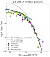 |
Fig. 1. 1.4 GHz LF for SFGs at z ∼ 0 from SEMPER obtained by using Delvecchio et al. (2021)qSFRFIR + UV relation with (black solid line) and without (dotted line) the correction defined in Eq. (11). Data for SFGs are from Mauch & Sadler (2007), Padovani et al. (2015), Condon et al. (2019) and Butler et al. (2019). The cyan line indicates the LF from the T-RECS simulation, with the shaded area representing its 1σ uncertainty. |
Fig. 2 shows the modelled 1.4 GHz radio LF for different redshift bins over the range 0.1 < z ≲ 5.7 (black solid lines). We compare our model with the determinations from Novak et al. (2017, green triangles), Enia et al. (2022, gold diamonds), van der Vlugt et al. (2022, blue circles), and van der Vlugt et al. (2023, purple circles). Our model successfully reproduces the observations across the full redshift range (0.1 < z < 5.7). We also compare our predictions with T-RECS ones. We note that the T-RECS LFs show significant offsets with respect to our LFs (up to ∼0.5 dex). Such offsets become increasingly prominent going to higher redshifts. This discrepancy may be due, at least in part, to the fact that the SFG population includes RQ AGNs in the T-RECS simulation (see also Sect. 4.4). Generally, our model better reproduces the observations, except for the highest redshift bin (4.6 < z < 5.7). Finally, we show the LFs we would obtain by implementing the SMFs from W23, which are based on a Double Schechter function fit (black dot-dashed lines). We notice a discrepancy with observations at the highest redshift bins, which we discuss in more detail in Sect. 4.2.
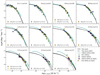 |
Fig. 2. 1.4 GHz LF for SFGs for different redshift bins (black solid lines) predicted by SEMPER adopting the Delvecchio et al. (2021) relation. Dot-dashed lines show how our model would change when considering the SMFs derived by W23 with a Double Schechter form. Eq. (11) is applied only for the first redshift bin. Data are from Novak et al. (2017), Enia et al. (2022), and van der Vlugt et al. (2022, 2023). Enia et al. (2022) and van der Vlugt et al. (2023) data include the contribution of ‘dark’ sources. The cyan lines and shaded areas are the predictions from the T-RECS simulation by Bonaldi et al. (2019, 2023) and the respective 1σ uncertainties. Note that data from Enia et al. (2022) spans redshift bins not matching the ones adopted by our model and shown in each panel’s legend. |
4.2. Massive galaxies
As previously discussed, W23 found a large number of massive and red SFGs, which are typically located at high redshift (z > 3) and are heavily dust-obscured (AV > 3). Such sources challenge galaxy formation and evolution simulations, which predict 1.8× fewer sources at 2.5 < z ≤ 5.5 over the same mass range (W23). Because of the deeper NIR UltraVISTA images, COSMOS2020 is more sensitive to faint red sources with respect to previous surveys conducted at optical/NIR wavelengths, which likely missed most of these objects (e.g. Simpson et al. 2014; Franco et al. 2018; Wang et al. 2019; Barrufet et al. 2023; Williams et al. 2024). A fraction of them were, however, observed at longer wavelengths. Such galaxies are usually referred to as ‘optically dark’ (Simpson et al. 2014; Wang et al. 2019; Gruppioni et al. 2020; Sun et al. 2021; Fudamoto et al. 2021; Smail et al. 2021; Talia et al. 2021; Enia et al. 2022; Shu et al. 2022; Behiri et al. 2023; van der Vlugt et al. 2023; Gentile et al. 2024; Williams et al. 2024), although various terminologies exist depending on their selection method (e.g. HST-dark, Rs-NIR dark, H-dropout, NIR-dark/faint, OIR-dark). In recent years, several observational studies (e.g. Wang et al. 2019; Gruppioni et al. 2020) have highlighted that this population of ‘dark’ galaxies can significantly impact the cosmic SFR density, with a contribution up to ∼40% the contribution of high-redshift Lyman-Break Galaxies (Talia et al. 2021; Enia et al. 2022; Behiri et al. 2023; van der Vlugt et al. 2023; Gentile et al. 2024).
Our model, derived from SMFs based on ultra-deep NIR observations, is sensitive to this red high-mass galaxy population and likely includes at least a fraction of dark (and/or extremely NIR faint) objects. Therefore, it is interesting to explore the link between massive and NIR-faint galaxies, accounted for in our model, and radio-selected SFG samples, which should be unbiased against optical colour.
In Fig. 3, we directly compare the SMFs presented in Appendix A and our 1.4 GHz LF predictions for the two latter redshift bins of Fig. 2. We note that when the double power law fit is used in the derivation of the LF, the model can reproduce the observations of high redshift (z ≳ 3.3) radio-selected samples (Novak et al. 2017; Enia et al. 2022; van der Vlugt et al. 2022, 2023). In contrast, the observed 1.4 GHz LFs are not reproduced when using a Double Schechter fit to the SMFs, which does not account for galaxies with M⋆ > 1011 M⊙. The observed discrepancy is more prominent when considering radio samples, including dark galaxies (Enia et al. 2022; van der Vlugt et al. 2023; red points). Remarkably, this comparison suggests that the high-z massive and red objects detected in excess in the NIR (W23) likely correspond to a population of bright radio sources at similar redshifts. This result is in line with observational studies (e.g. Talia et al. 2021; Enia et al. 2022; Behiri et al. 2023; Gentile et al. 2024) showing that radio band observations are sensitive to massive and obscured galaxies. This evidence further validates our choice to adopt a Double Power Law profile for the SMFs’ reconstruction.
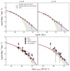 |
Fig. 3. This figure summarises the results presented in Sect. 4.2. The two top panels show the SMFs for the highest redshift bins discussed in this paper. The bottom panels show the LF at 1.4 GHz derived from our model in the same redshift bins. The yellow dashed and purple solid lines respectively indicate the predictions obtained when adopting a Double Schechter Function (W23) and a Double Power Law (this paper) for the SMFs fitting. The hatched grey area highlights the difference between the two curves. Data points are the same as in Fig. A.2 for the SMFs and Fig. 2 for the LFs, highlighting in red samples which include dark galaxies. |
Thanks to its unprecedented sensitivity at near and mid-infrared bands, JWST is finding significant numbers of massive, dust-obscured SFGs already in place at high redshifts (Barrufet et al. 2023; Labbé et al. 2023; Nelson et al. 2023; Pérez-González et al. 2023). Future deeper JWST observations (e.g. in the context of the COSMOS-Web survey, see Casey et al. 2023) will better characterise this population by reducing the existing uncertainties on their photometric redshifts and stellar masses (e.g. Barrufet et al. 2023). These observations will provide more stringent constraints that we can use to refine our model, possibly improving further the matching with the observed radio LFs at z > 4.
4.3. Number counts at 1.4 GHz
Fig. 4 shows the 1.4 GHz number counts predicted by our model by adopting Eq. (7). Our predictions agree with the number counts derived for SFGs by Bonato et al. (2021b, light blue triangles), and also reproduce the observed number counts for local galaxies obtained by Mauch & Sadler (2007, black crosses) at log S1.4 GHz ≳ 1 mJy. The overall trend is similar to the one of the Mancuso et al. (2017, pink solid line) model, even if we predict a higher (∼0.2 dex) number of SFGs at fluxes S1.4 GHz ≲ 0.5 mJy. The 1.4 GHz number counts from the T-RECS simulation are up to ∼0.7 dex higher than our predictions for S1.4 GHz ≳ 0.1 mJy, but are consistent with observations when including the contribution of RQ AGNs (Bonato et al. 2021b, dark blue triangles).
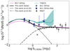 |
Fig. 4. 1.4 GHz Euclidean normalised differential number counts from SEMPER for SFGs (black solid line) obtained adopting the relation of Delvecchio et al. (2021). The dashed and dot-dashed lines represent the contribution for galaxies located respectively above and below z ∼ 0.05. The solid pink line is the prediction from Mancuso et al. (2017). Triangles are data from Bonato et al. (2021b) for SFGs (light blue) and SFGs and RQ sources combined (dark blue). In cyan, we display the predictions from the T-RECS simulation by Bonaldi et al. (2019, 2023). Black crosses show the number counts for local galaxies from Mauch & Sadler (2007). |
4.4. Luminosity functions at 150 MHz
Fig. 5 shows our predictions for the local (0.03 < z < 0.3) 150 MHz LF, compared with recent determinations at 150 and 610 MHz (Cochrane et al. 2023, purple diamonds; Sabater et al. 2019, empty green circles; Bonato et al. 2021a, gold triangles; Ocran et al. 2020a, blue squares). Moreover, we include the parametrised expression (dotted purple line) derived by Cochrane et al. (2023) adopting a modified Schechter function. The 150 MHz LF predictions presented in this section are derived using both the McCheyne et al. (2022, Eq. 8; black solid line) and the Delvecchio et al. (2021, Eq. 7; hatched grey area) FIRRC relations. The latter has been rescaled to 150 MHz using a range of spectral indexes (α = [ − 0.8, −0.6]), to better account for a realistic spectral index distribution around the typical SFG value of −0.7, and/or any spectral index variations with redshift (in the case of redshift-dependent LFs, see Fig. 6).
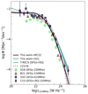 |
Fig. 5. 150 MHz LF for SFGs from SEMPER at z ∼ 0. The model is obtained from Eqs. (7) and (8) (hatched grey area) using a spectral index range of α = [ − 0.8, −0.6] and by applying Eq. (11). Data points are from Sabater et al. (2019), Bonato et al. (2021a) and Cochrane et al. (2023) at 150 MHz and Ocran et al. (2020a) at 640 MHz (rescaled assuming α = −0.7). The dotted line refers to the best-fit modified Schechter function presented in Cochrane et al. (2023). The shaded area is from the T-RECS simulation (Bonaldi et al. 2019, 2023). |
Our results agree very well with the determinations of Cochrane et al. (2023) and Ocran et al. (2020a). The data points from Sabater et al. (2019), Butler et al. (2019) and Bonato et al. (2021a) lie below our model and Cochrane et al. (2023) determinations (up to 1 dex offsets). As discussed in Cochrane et al. (2023), this difference likely arises from the lack of corrections for radio completeness in previous data sets and the different choices of redshift bins. This and the strong redshift evolution of the LFs may indeed explain the offset. The predictions from T-RECS (cyan shaded area) are roughly consistent with our model and with data from Cochrane et al. (2023). Fig. 5 also shows that the predictions derived from Eq. (7) are in better agreement with the predictions obtained from Eq. (8) when rescaled to 150 MHz using a flatter spectral index (α ≈ −0.6; see lower edge of the grey hatched area). This is consistent with what was found by McCheyne et al. (2022), i.e. that their FIRRC normalisation closely matches that of Delvecchio et al. (2021) when rescaled using a spectral index value α = −0.59.
Fig. 6 displays the 150 MHz LFs obtained for different redshift bins in the range 0.1 < z ≲ 5.7. Our predictions are compared with data from Cochrane et al. (2023), Bonato et al. (2021a) and Ocran et al. (2020a), as well as with predictions from the T-RECS simulation. The model based on Eq. (8) (black solid line) reproduces the observational data accurately up to redshift z ≈ 1.5. This suggests that the FIRRC from McCheyne et al. (2022), originally derived up to z ≈ 1, is able to represent the data up to slightly higher redshifts. At redshifts z ≳ 1.6 the observations better agree with the model predictions derived using Eq. (7) (hatched grey area). This may be due to the fact that Delvecchio et al. (2021) relation was derived from samples spanning a wider redshift range (1 < z < 4). As for ν = 1.4 GHz, we find good agreement between our model and the T-RECS simulation up to z ≈ 1.5. At higher redshifts, our model shifts towards lower luminosities compared to T-RECS. At z ≳ 3.3 the data better agree with T-RECS than with our model, which is located ∼0.5 dex below the observations from Cochrane et al. (2023) and Bonato et al. (2021a). This may be ascribed, at least partially, to the fact that both the T-RECS simulation and Cochrane et al. (2023) sample include the contribution from RQ AGNs. At redshift z > 4.6, both our model and T-RECS fall short. However, it is important to notice that the photometric redshifts of the LoTSS deep fields can be considered highly reliable only up to z ∼ 1.5 for SFGs (as extensively discussed in Duncan et al. 2021), implying that the highest-z bins of the LFs can be affected by large uncertainties.
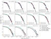 |
Fig. 6. 150 MHz LFs for SFGs at different redshift bins predicted by SEMPER. The model is derived by assuming the mass-dependent FIRRC from Delvecchio et al. (2021) (solid black line) and McCheyne et al. (2022) (hatched grey area). As in Fig. 2, Eq. (11) is applied only to the first redshift bin. Data points (symbols as in legend) are from Cochrane et al. (2023), Bonato et al. (2021a) and Ocran et al. (2020a). The latter are scaled from 610 MHz to 150 MHz assuming α = −0.7. Cyan lines and shaded areas are the predictions from the T-RECS simulation by Bonaldi et al. (2019, 2023) and their 1σ uncertainties, respectively. |
4.5. Number counts at 150 MHz
In Fig. 7, we show the number counts at ν = 150 MHz as derived from our model, compared with the predictions of the T-RECS simulation (cyan shaded area) and of the model by Mancuso et al. (2017) (pink solid line). We also present the number counts for SFGs and RQ-AGNs that we derived from the DR1 catalogues of the LoTSS deep fields (see Tab. 1). As for the 150 MHz LFs, the modelled counts are obtained adopting either the FIRRC described in Eq. (8) (McCheyne et al. 2022, black solid line) or the one described by Eq. (7) (Delvecchio et al. 2021, hatched grey area). Whichever FIRRC relation we adopt, our model agrees very well with the observed source counts. In particular, our model can better reproduce the decrease of the number counts observed at ≳1.5 mJy than the Mancuso et al. (2017) model. The T-RECS simulation lies above our predictions (and the observed source counts) by at least ∼0.3 dex overall. A better agreement with T-RECS is, however, observed in the range 0.1 ≲ S150 MHz ≲ 1 mJy, when we adopt the Delvecchio et al. (2021) FIRRC.
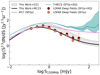 |
Fig. 7. 150 MHz Euclidean normalised differential number counts for SFGs from SEMPER. The solid black line (hatched area) represents our model obtained adopting Eq. (8) (Eq. 7, scaled to 150 MHz using a spectral index range −0.8 < α < −0.6). The cyan and pink solid lines represent predictions from the T-RECS simulation (Bonaldi et al. 2019, 2023) and the model from Mancuso et al. (2017), respectively. Circles are the differential source counts we computed from the LoTSS deep fields DR1 catalogues. |
5. Conclusions
In this paper, we have developed SEMPER, a semi-empirical model to predict radio LFs and number counts for SFGs. Our model combines the evolving SMFs for SFGs, based on the recent deep NIR data from the COSMOS2020 catalogue (W23), with up-to-date observed scaling relations, such as the galaxy main sequence from Popesso et al. (2023) and the mass- and redshift-dependent FIRRC from Delvecchio et al. (2021) and McCheyne et al. (2022). We refitted the redshift-dependent W23 SMFs with a Double Power Law function instead of with the Double Schechter function originally adopted by the authors. We modelled the fit parameters in the range 0 < z < 5 and obtained the time and shape evolution of the SMFs.
We tested our model against radio data at two reference frequencies: 1.4 GHz and 150 MHz. In general, we find remarkably good agreement with the latest observational constraints on LFs and number counts from the JVLA, LOFAR, GMRT, WSRT and ATCA. Our main results can be summarised as follows:
-
Our SMFs, reconstructed via a Double Power Law function, nicely reproduce observations for all the redshift bins, including the observed massive galaxies (M⋆ ≳ 1011 M⊙) at high redshifts (z ≳ 2.5), which were attributed by W23 to a novel population of dust-obscured SFGs, only revealed thanks to ultra-deep NIR imaging in the COSMOS field. This population could not be reproduced by a Double Schechter function fitting.
-
Our predictions align with observational determinations of the 1.4 GHz LFs up to redshift z ∼ 5, while deviating from the T-RECS sky simulation at z ≳ 1, particularly at bright and faint luminosities.
-
Our model can reproduce the observed 1.4 GHz LFs obtained for samples of radio-selected massive and dust-obscured SFGs at z > 3.5, some of which contain a fraction of optically dark galaxies. This indirectly suggests a natural link between this population and the radio-bright SFGs population observed at high redshift in deep radio fields.
-
The 1.4 GHz normalised number counts are well in agreement with determinations for local and high redshift SFGs obtained from the NVSS survey (Mauch & Sadler 2007) and WSRT deep observations of the Lockman Hole (Prandoni et al. 2018; Bonato et al. 2021b), respectively. Our model shows a similar trend to the one of Mancuso et al. (2017), but predicts a slightly higher (∼0.2 dex) number of SFGs for S1.4 GHz ≲ 0.5 mJy, while it deviates from the T-RECS predictions at S1.4 GHz ≳ 0.1 mJy.
-
We find good agreement between our predicted and observed LFs also at low frequency (ν = 150 MHz), particularly when compared with the recent determinations from the LoTSS deep fields (Cochrane et al. 2023). Using the FIRRC of McCheyne et al. (2022) yields better results for z ≲ 1.5, while better consistency is found with the data at higher redshifts when using the Delvecchio et al. (2021) relation. The origin of this discrepancy is likely associated with the different redshift ranges sampled by the two correlations. At z ≳ 3.3, the LFs observed in the LoTSS deep fields show an excess with respect to our model predictions. We attribute this discrepancy to either larger photometric redshift uncertainties in the LoTSS-Deep DR1 radio catalogues or to the fact that both SFGs and RQ AGN are included in the observed LFs.
-
We derive the 150 MHz number counts for SFGs and RQ AGN from the LoTSS deep fields DR1 catalogues. Our 150 MHz number count predictions closely match the observed LoTSS-deep number counts either when we consider SFGs alone or when we include RQ AGNs. We only find partial agreement between our results and what is predicted by Mancuso et al. (2017), as their model produces flatter counts at S150 MHz ≳ 1.5 mJy. The T-RECS simulation, on the other hand, predicts higher counts than our model over the entire flux range explored.
Our predictions can be further tested with upcoming deep radio continuum surveys planned for SKA precursors (Norris et al. 2013) and, on a longer timescale, for the SKA (Prandoni & Seymour 2015). We also plan to update our model by exploiting optical/NIR JWST observations, which will soon provide new SMFs expanding the redshift and mass ranges explored so far.
Acknowledgments
M. G. acknowledges support from INAF under the Large Grant 2022 funding scheme (project “MeerKAT and LOFAR Team up: a Unique Radio Window on Galaxy/AGN co-Evolution”). M. B. acknowledges support from INAF under the mini-grant “A systematic search for ultra-bright high-z strongly lensed galaxies in Planck catalogues”. L.B. acknowledges financial support from the German Excellence Strategy via the Heidelberg Cluster of Excellence (EXC 2181 – 390900948) STRUCTURES. A. L. has been supported by: European Union – NextGenerationEU under the PRIN MUR 2022 project n. 20224JR28W “Charting unexplored avenues in Dark Matter”; INAF Large Grant 2022 funding scheme with the project “MeerKAT and LOFAR Team up: a Unique Radio Window on Galaxy/AGN co-Evolution”; INAF GO-GTO Normal 2023 funding scheme with the project “Serendipitous H-ATLAS-fields Observations of Radio Extragalactic Sources (SHORES)”; project “Data Science methods for MultiMessenger Astrophysics & Multi-Survey Cosmology” funded by the Italian Ministry of University and Research, Programmazione triennale 2021/2023 (DM n.2503 dd. 9 December 2019), Programma Congiunto Scuole; Italian Research Center on High Performance Computing Big Data and Quantum Computing (ICSC), project funded by European Union – NextGenerationEU – and National Recovery and Resilience Plan (NRRP) – Mission 4 Component 2 within the activities of Spoke 3 (Astrophysics and Cosmos Observations).
References
- Algera, H. S. B., van der Vlugt, D., Hodge, J. A., et al. 2020, ApJ, 903, 139 [Google Scholar]
- An, F., Vaccari, M., Smail, I., et al. 2021, MNRAS, 507, 2643 [NASA ADS] [CrossRef] [Google Scholar]
- Barrufet, L., Oesch, P. A., Weibel, A., et al. 2023, MNRAS, 522, 449 [NASA ADS] [CrossRef] [Google Scholar]
- Basu, A., Wadadekar, Y., Beelen, A., et al. 2015, ApJ, 803, 51 [NASA ADS] [CrossRef] [Google Scholar]
- Behiri, M., Talia, M., Cimatti, A., et al. 2023, ApJ, 957, 63 [NASA ADS] [CrossRef] [Google Scholar]
- Behroozi, P. S., Wechsler, R. H., & Conroy, C. 2013, ApJ, 770, 57 [NASA ADS] [CrossRef] [Google Scholar]
- Behroozi, P., Wechsler, R. H., Hearin, A. P., & Conroy, C. 2019, MNRAS, 488, 3143 [NASA ADS] [CrossRef] [Google Scholar]
- Bell, E. F. 2003, ApJ, 586, 794 [Google Scholar]
- Best, P. N., Kondapally, R., Williams, W. L., et al. 2023, MNRAS, 523, 1729 [NASA ADS] [CrossRef] [Google Scholar]
- Béthermin, M., Daddi, E., Magdis, G., et al. 2012, ApJ, 757, L23 [Google Scholar]
- Bisigello, L., Caputi, K. I., Grogin, N., & Koekemoer, A. 2018, A&A, 609, A82 [NASA ADS] [CrossRef] [EDP Sciences] [Google Scholar]
- Bisigello, L., Vallini, L., Gruppioni, C., et al. 2022, A&A, 666, A193 [NASA ADS] [CrossRef] [EDP Sciences] [Google Scholar]
- Boco, L., Lapi, A., Chruslinska, M., et al. 2021, ApJ, 907, 110 [NASA ADS] [CrossRef] [Google Scholar]
- Boco, L., Lapi, A., Shankar, F., et al. 2023, ApJ, 954, 97 [NASA ADS] [CrossRef] [Google Scholar]
- Bonaldi, A., Bonato, M., Galluzzi, V., et al. 2019, MNRAS, 482, 2 [Google Scholar]
- Bonaldi, A., Hartley, P., Ronconi, T., De Zotti, G., & Bonato, M. 2023, MNRAS, 524, 993 [CrossRef] [Google Scholar]
- Bonato, M., Negrello, M., Mancuso, C., et al. 2017, MNRAS, 469, 1912 [Google Scholar]
- Bonato, M., Prandoni, I., De Zotti, G., et al. 2021a, A&A, 656, A48 [NASA ADS] [CrossRef] [EDP Sciences] [Google Scholar]
- Bonato, M., Prandoni, I., De Zotti, G., et al. 2021b, MNRAS, 500, 22 [Google Scholar]
- Bourne, N., Dunne, L., Ivison, R. J., et al. 2011, MNRAS, 410, 1155 [Google Scholar]
- Brinchmann, J., Charlot, S., White, S. D. M., et al. 2004, MNRAS, 351, 1151 [Google Scholar]
- Buat, V., Noll, S., Burgarella, D., et al. 2012, A&A, 545, A141 [NASA ADS] [CrossRef] [EDP Sciences] [Google Scholar]
- Burgarella, D., Buat, V., Gruppioni, C., et al. 2013, A&A, 554, A70 [NASA ADS] [CrossRef] [EDP Sciences] [Google Scholar]
- Butler, A., Huynh, M., Kapińska, A., et al. 2019, A&A, 625, A111 [NASA ADS] [CrossRef] [EDP Sciences] [Google Scholar]
- Calistro Rivera, G., Williams, W. L., Hardcastle, M. J., et al. 2017, MNRAS, 469, 3468 [Google Scholar]
- Caputi, K. I., Deshmukh, S., Ashby, M. L. N., et al. 2017, ApJ, 849, 45 [Google Scholar]
- Casey, C. M., Kartaltepe, J. S., Drakos, N. E., et al. 2023, ApJ, 954, 31 [NASA ADS] [CrossRef] [Google Scholar]
- Ceraj, L., Smolčić, V., Delvecchio, I., et al. 2018, A&A, 620, A192 [NASA ADS] [CrossRef] [EDP Sciences] [Google Scholar]
- Chabrier, G. 2003, PASP, 115, 763 [Google Scholar]
- Chapman, S. C., Smail, I., Blain, A. W., & Ivison, R. J. 2004, ApJ, 614, 671 [Google Scholar]
- Chi, X., & Wolfendale, A. W. 1990, MNRAS, 245, 101 [Google Scholar]
- Cochrane, R. K., Kondapally, R., Best, P. N., et al. 2023, MNRAS, 523, 6082 [NASA ADS] [CrossRef] [Google Scholar]
- Condon, J. J. 1992, ARA&A, 30, 575 [Google Scholar]
- Condon, J. J., Cotton, W. D., Greisen, E. W., et al. 1998, AJ, 115, 1693 [Google Scholar]
- Condon, J. J., Cotton, W. D., & Broderick, J. J. 2002, AJ, 124, 675 [Google Scholar]
- Condon, J. J., Matthews, A. M., & Broderick, J. J. 2019, ApJ, 872, 148 [NASA ADS] [CrossRef] [Google Scholar]
- Cucciati, O., Tresse, L., Ilbert, O., et al. 2012, A&A, 539, A31 [NASA ADS] [CrossRef] [EDP Sciences] [Google Scholar]
- Daddi, E., Dickinson, M., Morrison, G., et al. 2007, ApJ, 670, 156 [NASA ADS] [CrossRef] [Google Scholar]
- Daddi, E., Delvecchio, I., Dimauro, P., et al. 2022, A&A, 661, L7 [NASA ADS] [CrossRef] [EDP Sciences] [Google Scholar]
- Davidzon, I., Ilbert, O., Laigle, C., et al. 2017, A&A, 605, A70 [NASA ADS] [CrossRef] [EDP Sciences] [Google Scholar]
- de Zotti, G., Massardi, M., Negrello, M., & Wall, J. 2010, A&ARv, 18, 1 [CrossRef] [Google Scholar]
- De Zotti, G., Bonato, M., Giulietti, M., et al. 2024, A&A, 689, A272 [NASA ADS] [CrossRef] [EDP Sciences] [Google Scholar]
- Delhaize, J., Smolčić, V., Delvecchio, I., et al. 2017, A&A, 602, A4 [NASA ADS] [CrossRef] [EDP Sciences] [Google Scholar]
- Delvecchio, I., Daddi, E., Sargent, M. T., et al. 2021, A&A, 647, A123 [NASA ADS] [CrossRef] [EDP Sciences] [Google Scholar]
- Driver, S. P., Hill, D. T., Kelvin, L. S., et al. 2011, MNRAS, 413, 971 [Google Scholar]
- Driver, S. P., Bellstedt, S., Robotham, A. S. G., et al. 2022, MNRAS, 513, 439 [NASA ADS] [CrossRef] [Google Scholar]
- Duchesne, S. W., Grundy, J. A., Heald, G. H., et al. 2024, PASA, 41, e003 [NASA ADS] [CrossRef] [Google Scholar]
- Duncan, K. J., Kondapally, R., Brown, M. J. I., et al. 2021, A&A, 648, A4 [EDP Sciences] [Google Scholar]
- Dunlop, J. S., McLure, R. J., Biggs, A. D., et al. 2017, MNRAS, 466, 861 [Google Scholar]
- Enia, A., Talia, M., Pozzi, F., et al. 2022, ApJ, 927, 204 [NASA ADS] [CrossRef] [Google Scholar]
- Euclid Collaboration (Scaramella, R., et al.) 2022, A&A, 662, A112 [NASA ADS] [CrossRef] [EDP Sciences] [Google Scholar]
- Fitt, A. J., Alexander, P., & Cox, M. J. 1988, MNRAS, 233, 907 [Google Scholar]
- Foreman-Mackey, D., Hogg, D. W., Lang, D., & Goodman, J. 2013, PASP, 125, 306 [Google Scholar]
- Franco, M., Elbaz, D., Béthermin, M., et al. 2018, A&A, 620, A152 [NASA ADS] [CrossRef] [EDP Sciences] [Google Scholar]
- Fu, H., Shankar, F., Ayromlou, M., et al. 2022, MNRAS, 516, 3206 [NASA ADS] [CrossRef] [Google Scholar]
- Fudamoto, Y., Oesch, P. A., Schouws, S., et al. 2021, Nature, 597, 489 [CrossRef] [Google Scholar]
- Gentile, F., Talia, M., Behiri, M., et al. 2024, ApJ, 962, 26 [NASA ADS] [CrossRef] [Google Scholar]
- Gruppioni, C., Béthermin, M., Loiacono, F., et al. 2020, A&A, 643, A8 [NASA ADS] [CrossRef] [EDP Sciences] [Google Scholar]
- Grylls, P. J., Shankar, F., Zanisi, L., & Bernardi, M. 2019, MNRAS, 483, 2506 [NASA ADS] [CrossRef] [Google Scholar]
- Gürkan, G., Hardcastle, M. J., Smith, D. J. B., et al. 2018, MNRAS, 475, 3010 [Google Scholar]
- Helfand, D. J., White, R. L., & Becker, R. H. 2015, ApJ, 801, 26 [NASA ADS] [CrossRef] [Google Scholar]
- Helou, G. 1986, ApJ, 311, L33 [Google Scholar]
- Helou, G., Soifer, B. T., & Rowan-Robinson, M. 1985, ApJ, 298, L7 [Google Scholar]
- Henriques, B. M. B., Yates, R. M., Fu, J., et al. 2020, MNRAS, 491, 5795 [NASA ADS] [CrossRef] [Google Scholar]
- Heywood, I., Jarvis, M. J., Hale, C. L., et al. 2022, MNRAS, 509, 2150 [Google Scholar]
- Hurley, P. D., Oliver, S., Betancourt, M., et al. 2017, MNRAS, 464, 885 [Google Scholar]
- Ilbert, O., Arnouts, S., Le Floc’h, E., et al. 2015, A&A, 579, A2 [NASA ADS] [CrossRef] [EDP Sciences] [Google Scholar]
- Ivison, R. J., Alexander, D. M., Biggs, A. D., et al. 2010a, MNRAS, 402, 245 [Google Scholar]
- Ivison, R. J., Magnelli, B., Ibar, E., et al. 2010b, A&A, 518, L31 [NASA ADS] [CrossRef] [EDP Sciences] [Google Scholar]
- Jannuzi, B. T., & Dey, A. 1999, ASP Conf. Ser., 191, 111 [Google Scholar]
- Jarrett, T. H., Chester, T., Cutri, R., et al. 2000, AJ, 119, 2498 [Google Scholar]
- Jarvis, M. J., Smith, D. J. B., Bonfield, D. G., et al. 2010, MNRAS, 409, 92 [Google Scholar]
- Jarvis, M., Seymour, N., Afonso, J., et al. 2015, Advancing Astrophysics with the Square Kilometre Array (AASKA14), 68 [Google Scholar]
- Jarvis, M., Taylor, R., Agudo, I., et al. 2016, MeerKAT Science: On the Pathway to the SKA, 6 [Google Scholar]
- Jin, S., Daddi, E., Liu, D., et al. 2018, ApJ, 864, 56 [Google Scholar]
- Johnston, S., Bailes, M., Bartel, N., et al. 2007, PASA, 24, 174 [NASA ADS] [CrossRef] [Google Scholar]
- Jones, D. H., Saunders, W., Colless, M., et al. 2004, MNRAS, 355, 747 [NASA ADS] [CrossRef] [Google Scholar]
- Kennicutt, R. C., & Evans, N. J. 2012, ARA&A, 50, 531 [NASA ADS] [CrossRef] [Google Scholar]
- Klein, U., Wielebinski, R., & Thuan, T. X. 1984, A&A, 141, 241 [NASA ADS] [Google Scholar]
- Kondapally, R., Best, P. N., Hardcastle, M. J., et al. 2021, A&A, 648, A3 [EDP Sciences] [Google Scholar]
- Labbé, I., van Dokkum, P., Nelson, E., et al. 2023, Nature, 616, 266 [CrossRef] [Google Scholar]
- Lacey, C. G., Baugh, C. M., Frenk, C. S., et al. 2016, MNRAS, 462, 3854 [Google Scholar]
- Lacki, B. C., & Thompson, T. A. 2010, ApJ, 717, 196 [Google Scholar]
- Lacy, M., Baum, S. A., Chandler, C. J., et al. 2020, PASP, 132, 035001 [Google Scholar]
- Lagos, C. D. P., Tobar, R. J., Robotham, A. S. G., et al. 2018, MNRAS, 481, 3573 [CrossRef] [Google Scholar]
- Lapi, A., Pantoni, L., Boco, L., & Danese, L. 2020, ApJ, 897, 81 [NASA ADS] [CrossRef] [Google Scholar]
- Lapi, A., Boco, L., & Shankar, F. 2025, Encyclopedia of Astrophysics, Elsevier, in press [arXiv:2502.12764] [Google Scholar]
- Le Floc’h, E., Aussel, H., Ilbert, O., et al. 2009, ApJ, 703, 222 [Google Scholar]
- Leja, J., Speagle, J. S., Ting, Y.-S., et al. 2022, ApJ, 936, 165 [NASA ADS] [CrossRef] [Google Scholar]
- Leslie, S. K., Schinnerer, E., Liu, D., et al. 2020, ApJ, 899, 58 [Google Scholar]
- Lockman, F. J., Jahoda, K., & McCammon, D. 1986, ApJ, 302, 432 [Google Scholar]
- Lonsdale Persson, C. J., & Helou, G. 1987, ApJ, 314, 513 [NASA ADS] [CrossRef] [Google Scholar]
- Lutz, D., Poglitsch, A., Altieri, B., et al. 2011, A&A, 532, A90 [NASA ADS] [CrossRef] [EDP Sciences] [Google Scholar]
- Magnelli, B., Ivison, R. J., Lutz, D., et al. 2015, A&A, 573, A45 [NASA ADS] [CrossRef] [EDP Sciences] [Google Scholar]
- Mancuso, C., Lapi, A., Cai, Z.-Y., et al. 2015, ApJ, 810, 72 [Google Scholar]
- Mancuso, C., Lapi, A., Shi, J., et al. 2016a, ApJ, 823, 128 [NASA ADS] [CrossRef] [Google Scholar]
- Mancuso, C., Lapi, A., Shi, J., et al. 2016b, ApJ, 833, 152 [NASA ADS] [CrossRef] [Google Scholar]
- Mancuso, C., Lapi, A., Prandoni, I., et al. 2017, ApJ, 842, 95 [Google Scholar]
- Mannucci, F., Cresci, G., Maiolino, R., Marconi, A., & Gnerucci, A. 2010, MNRAS, 408, 2115 [NASA ADS] [CrossRef] [Google Scholar]
- Massardi, M., Bonaldi, A., Negrello, M., et al. 2010, MNRAS, 404, 532 [NASA ADS] [Google Scholar]
- Mauch, T., & Sadler, E. M. 2007, MNRAS, 375, 931 [Google Scholar]
- McCheyne, I., Oliver, S., Sargent, M., et al. 2022, A&A, 662, A100 [NASA ADS] [CrossRef] [EDP Sciences] [Google Scholar]
- McCracken, H. J., Milvang-Jensen, B., Dunlop, J., et al. 2012, A&A, 544, A156 [NASA ADS] [CrossRef] [EDP Sciences] [Google Scholar]
- Molnár, D. C., Sargent, M. T., Leslie, S., et al. 2021, MNRAS, 504, 118 [CrossRef] [Google Scholar]
- Moneti, A., McCracken, H. J., Hudelot, W., et al. 2023, VizieR Online Data Catalog: II/373 [Google Scholar]
- Moster, B. P., Naab, T., & White, S. D. M. 2013, MNRAS, 428, 3121 [Google Scholar]
- Moster, B. P., Naab, T., & White, S. D. M. 2018, MNRAS, 477, 1822 [Google Scholar]
- Murphy, E. J., Condon, J. J., Schinnerer, E., et al. 2011, ApJ, 737, 67 [Google Scholar]
- Nelson, E. J., Suess, K. A., Bezanson, R., et al. 2023, ApJ, 948, L18 [NASA ADS] [CrossRef] [Google Scholar]
- Noeske, K. G., Weiner, B. J., Faber, S. M., et al. 2007, ApJ, 660, L43 [CrossRef] [Google Scholar]
- Norris, R. P., Afonso, J., Bacon, D., et al. 2013, PASA, 30, e020 [NASA ADS] [CrossRef] [Google Scholar]
- Norris, R. P., Marvil, J., Collier, J. D., et al. 2021, PASA, 38, e046 [NASA ADS] [CrossRef] [Google Scholar]
- Novak, M., Smolčić, V., Delhaize, J., et al. 2017, A&A, 602, A5 [NASA ADS] [CrossRef] [EDP Sciences] [Google Scholar]
- Ocran, E. F., Taylor, A. R., Vaccari, M., et al. 2020a, MNRAS, 491, 5911 [NASA ADS] [CrossRef] [Google Scholar]
- Ocran, E. F., Taylor, A. R., Vaccari, M., Ishwara-Chandra, C. H., & Prandoni, I. 2020b, MNRAS, 491, 1127 [Google Scholar]
- Ocran, E. F., Vaccari, M., Stil, J. M., et al. 2023, MNRAS, 524, 5229 [CrossRef] [Google Scholar]
- Oke, J. B. 1974, ApJS, 27, 21 [Google Scholar]
- Oliver, S., Rowan-Robinson, M., Alexander, D. M., et al. 2000, MNRAS, 316, 749 [Google Scholar]
- Oliver, S. J., Bock, J., Altieri, B., et al. 2012, MNRAS, 424, 1614 [NASA ADS] [CrossRef] [Google Scholar]
- Padovani, P. 2016, A&ARv, 24, 13 [Google Scholar]
- Padovani, P., Bonzini, M., Kellermann, K. I., et al. 2015, MNRAS, 452, 1263 [Google Scholar]
- Pannella, M., Elbaz, D., Daddi, E., et al. 2015, ApJ, 807, 141 [Google Scholar]
- Pantoni, L., Lapi, A., Massardi, M., Goswami, S., & Danese, L. 2019, ApJ, 880, 129 [NASA ADS] [CrossRef] [Google Scholar]
- Parente, M., Ragone-Figueroa, C., Granato, G. L., & Lapi, A. 2023, MNRAS, 521, 6105 [NASA ADS] [CrossRef] [Google Scholar]
- Pearson, W. J., Wang, L., Hurley, P. D., et al. 2018, A&A, 615, A146 [NASA ADS] [CrossRef] [EDP Sciences] [Google Scholar]
- Peng, Y.-J., Lilly, S. J., Kovač, K., et al. 2010, ApJ, 721, 193 [Google Scholar]
- Pérez-González, P. G., Barro, G., Annunziatella, M., et al. 2023, ApJ, 946, L16 [CrossRef] [Google Scholar]
- Popesso, P., Concas, A., Morselli, L., et al. 2019a, MNRAS, 483, 3213 [Google Scholar]
- Popesso, P., Morselli, L., Concas, A., et al. 2019b, MNRAS, 490, 5285 [Google Scholar]
- Popesso, P., Concas, A., Cresci, G., et al. 2023, MNRAS, 519, 1526 [Google Scholar]
- Prandoni, I., & Seymour, N. 2015, Advancing Astrophysics with the Square Kilometre Array (AASKA14), 67 [Google Scholar]
- Prandoni, I., Guglielmino, G., Morganti, R., et al. 2018, MNRAS, 481, 4548 [Google Scholar]
- Price, R., & Duric, N. 1992, ApJ, 401, 81 [NASA ADS] [CrossRef] [Google Scholar]
- Read, S. C., Smith, D. J. B., Gürkan, G., et al. 2018, MNRAS, 480, 5625 [Google Scholar]
- Renzini, A., & Peng, Y.-J. 2015, ApJ, 801, L29 [Google Scholar]
- Rinaldi, P., Navarro-Carrera, R., Caputi, K. I., et al. 2025, ApJ, 981, 161 [Google Scholar]
- Rodighiero, G., Daddi, E., Baronchelli, I., et al. 2011, ApJ, 739, L40 [Google Scholar]
- Rodighiero, G., Renzini, A., Daddi, E., et al. 2014, MNRAS, 443, 19 [Google Scholar]
- Rodighiero, G., Brusa, M., Daddi, E., et al. 2015, ApJ, 800, L10 [Google Scholar]
- Sabater, J., Best, P. N., Hardcastle, M. J., et al. 2019, A&A, 622, A17 [NASA ADS] [CrossRef] [EDP Sciences] [Google Scholar]
- Sabater, J., Best, P. N., Tasse, C., et al. 2021, A&A, 648, A2 [EDP Sciences] [Google Scholar]
- Sargent, M. T., Schinnerer, E., Murphy, E., et al. 2010, ApJ, 714, L190 [Google Scholar]
- Sargent, M. T., Béthermin, M., Daddi, E., & Elbaz, D. 2012, ApJ, 747, L31 [Google Scholar]
- Schleicher, D. R. G., & Beck, R. 2016, A&A, 593, A77 [NASA ADS] [CrossRef] [EDP Sciences] [Google Scholar]
- Schreiber, C., Pannella, M., Elbaz, D., et al. 2015, A&A, 575, A74 [NASA ADS] [CrossRef] [EDP Sciences] [Google Scholar]
- Shimwell, T. W., Röttgering, H. J. A., Best, P. N., et al. 2017, A&A, 598, A104 [NASA ADS] [CrossRef] [EDP Sciences] [Google Scholar]
- Shimwell, T. W., Tasse, C., Hardcastle, M. J., et al. 2019, A&A, 622, A1 [NASA ADS] [CrossRef] [EDP Sciences] [Google Scholar]
- Shimwell, T. W., Hardcastle, M. J., Tasse, C., et al. 2022, A&A, 659, A1 [NASA ADS] [CrossRef] [EDP Sciences] [Google Scholar]
- Shu, X., Yang, L., Liu, D., et al. 2022, ApJ, 926, 155 [NASA ADS] [CrossRef] [Google Scholar]
- Shuntov, M., Ilbert, O., Toft, S., et al. 2025, A&A, 695, A20 [NASA ADS] [CrossRef] [EDP Sciences] [Google Scholar]
- Simpson, J. M., Swinbank, A. M., Smail, I., et al. 2014, ApJ, 788, 125 [Google Scholar]
- Sinha, A., Basu, A., Datta, A., & Chakraborty, A. 2022, MNRAS, 514, 4343 [NASA ADS] [CrossRef] [Google Scholar]
- Skrutskie, M. F., Cutri, R. M., Stiening, R., et al. 2006, AJ, 131, 1163 [NASA ADS] [CrossRef] [Google Scholar]
- Smail, I., Dudzevičiūtė, U., Stach, S. M., et al. 2021, MNRAS, 502, 3426 [NASA ADS] [CrossRef] [Google Scholar]
- Smith, D. J. B., Haskell, P., Gürkan, G., et al. 2021, A&A, 648, A6 [EDP Sciences] [Google Scholar]
- Smolčić, V., Schinnerer, E., Scodeggio, M., et al. 2008, ApJS, 177, 14 [Google Scholar]
- Smolčić, V., Novak, M., Bondi, M., et al. 2017, A&A, 602, A1 [Google Scholar]
- Speagle, J. S., Steinhardt, C. L., Capak, P. L., & Silverman, J. D. 2014, ApJS, 214, 15 [Google Scholar]
- Sun, F., Egami, E., Pérez-González, P. G., et al. 2021, ApJ, 922, 114 [NASA ADS] [CrossRef] [Google Scholar]
- Tabatabaei, F. S., Martinsson, T. P. K., Knapen, J. H., et al. 2016, ApJ, 818, L10 [NASA ADS] [CrossRef] [Google Scholar]
- Talia, M., Cimatti, A., Giulietti, M., et al. 2021, ApJ, 909, 23 [NASA ADS] [CrossRef] [Google Scholar]
- Tasse, C., Shimwell, T., Hardcastle, M. J., et al. 2021, A&A, 648, A1 [EDP Sciences] [Google Scholar]
- Taylor, A. J., Barger, A. J., Cowie, L. L., et al. 2023, ApJS, 266, 24 [Google Scholar]
- Thorne, J. E., Robotham, A. S. G., Davies, L. J. M., et al. 2021, MNRAS, 505, 540 [NASA ADS] [CrossRef] [Google Scholar]
- Vaccari, M. 2015, in SALT Science Conference 2015 (SSC2015), eds. D. Buckley, & A. Schroeder, 17 [Google Scholar]
- van der Vlugt, D., Algera, H. S. B., Hodge, J. A., et al. 2021, ApJ, 907, 5 [NASA ADS] [CrossRef] [Google Scholar]
- van der Vlugt, D., Hodge, J. A., Algera, H. S. B., et al. 2022, ApJ, 941, 10 [NASA ADS] [CrossRef] [Google Scholar]
- van der Vlugt, D., Hodge, J. A., Jin, S., et al. 2023, ApJ, 951, 131 [NASA ADS] [CrossRef] [Google Scholar]
- van Haarlem, M. P., Wise, M. W., Gunst, A. W., et al. 2013, A&A, 556, A2 [NASA ADS] [CrossRef] [EDP Sciences] [Google Scholar]
- Vogelsberger, M., Marinacci, F., Torrey, P., & Puchwein, E. 2020, Nat. Rev. Phys., 2, 42 [Google Scholar]
- Wang, L., Gao, F., Duncan, K. J., et al. 2019, A&A, 631, A109 [NASA ADS] [CrossRef] [EDP Sciences] [Google Scholar]
- Weaver, J. R., Kauffmann, O. B., Ilbert, O., et al. 2022, ApJS, 258, 11 [NASA ADS] [CrossRef] [Google Scholar]
- Weaver, J. R., Davidzon, I., Toft, S., et al. 2023, A&A, 677, A184 [NASA ADS] [CrossRef] [EDP Sciences] [Google Scholar]
- Whitaker, K. E., Franx, M., Leja, J., et al. 2014, ApJ, 795, 104 [NASA ADS] [CrossRef] [Google Scholar]
- Whitaker, K. E., Pope, A., Cybulski, R., et al. 2017, ApJ, 850, 208 [NASA ADS] [CrossRef] [Google Scholar]
- Whittam, I. H., Jarvis, M. J., Hale, C. L., et al. 2022, MNRAS, 516, 245 [NASA ADS] [CrossRef] [Google Scholar]
- Williams, C. C., Alberts, S., Ji, Z., et al. 2024, ApJ, 968, 34 [NASA ADS] [CrossRef] [Google Scholar]
- Yun, M. S., Reddy, N. A., & Condon, J. J. 2001, ApJ, 554, 803 [Google Scholar]
Appendix A: Fitting the SMFs
Here we detail the fitting procedure of the observed SMFs of W23 and Driver et al. (2022) at different redshift bins. Our MCMC maximises the likelihood:
where ℳ(θ) are the expectations from the empirical model compared with the observed data y and their uncertainties σy. We adopt flat priors (π(θ)) for each parameter, initialised to the average value inside the reasonably large intervals: −1 ≤ α ≤ 0, 0 ≤ β ≤ 4 and 9 ≤ log M0(M⊙)≤12.5 to allow the chain to span a sufficient range of values. We find the posterior distribution 𝒫(θ)∝ℒπ(θ) to be well-sampled by adopting 500 walkers and 5000 iterations. To allow the chain to reach statistical equilibrium, we discard the first 500 iterations of the MCMC, corresponding to 10% of the total number of iterations. To allow the chain to converge, we fixed the normalisation of the second power-law to the value logΦ2 = 3.5 for all the redshift bins. Because of the lack of data points in the low-mass regime at z > 2.5 the parameter α is fixed at the maximum likelihood value of the preceding redshift bin (2.0 < z ≤ 2.5). Analogously, logΦ1 is fixed for z > 3.5. Fig. A.1 and Fig. A.2 show the resulting fitting solutions corresponding to the median posterior distribution and maximum likelihood parameters for the local and high-z SMFs, respectively. Our solutions are compared with the results obtained by Driver et al. (2022) (for the local SMF) and W23 by adopting a Single and Double Schechter profile, respectively. In Tab. A.1, we report the values of the best-fit parameters for the Double Power Law profile obtained from our analysis. The trend of the observed data is well reproduced by the Double Power Law function for all the redshift bins. In particular, it traces the high-masses points for z > 3, where the Double Schechter profile fails. Additionally, we fit the evolution of the parameters obtained from the fit at fixed redshift bins. This is done to retrieve the time and shape evolution of the SMF in the redshift range 0 < z < 5. We note that the redshift evolution of our resulting parameters cannot be well reproduced with a simple polynomial function. For this reason, we adopt a cubic spline fit with the number of knots equal to the number of redshift bins.
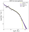 |
Fig. A.1. Results of the fit of a Double Power Law (dark blue curve) to the observed SMFs for local (z < 0.08) SFGs from Driver et al. (2022). Solid lines refer to the median of the posterior distribution, while dotted lines represent the maximum likelihood model. Shaded areas represent the 1- and 2-σ uncertainty interval obtained from the 2nd, 16th, 84th and 97th percentiles of the posterior distribution. Our fits are compared to the results of Driver et al. (2022) (green curve) inferred from a single Schechter function. Points are the observed SMFs for local SFGs of Driver et al. (2022). |
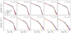 |
Fig. A.2. Same as Fig. A.1 but for the observed SMFs for SFGs of W23 in different redshift bins. Our fits (purple lines) are compared to the results of W23 (gold curves) for the double (z < 3) and single (z > 3) Schechter model. Points are the observed SMFs for SFGs of W23. |
List of the parameters obtained by fitting the double power-law profile to W23 SMFs data.
All Tables
List of the parameters obtained by fitting the double power-law profile to W23 SMFs data.
All Figures
|
Fig. 1. 1.4 GHz LF for SFGs at z ∼ 0 from SEMPER obtained by using Delvecchio et al. (2021)qSFRFIR + UV relation with (black solid line) and without (dotted line) the correction defined in Eq. (11). Data for SFGs are from Mauch & Sadler (2007), Padovani et al. (2015), Condon et al. (2019) and Butler et al. (2019). The cyan line indicates the LF from the T-RECS simulation, with the shaded area representing its 1σ uncertainty. |
| In the text | |
|
Fig. 2. 1.4 GHz LF for SFGs for different redshift bins (black solid lines) predicted by SEMPER adopting the Delvecchio et al. (2021) relation. Dot-dashed lines show how our model would change when considering the SMFs derived by W23 with a Double Schechter form. Eq. (11) is applied only for the first redshift bin. Data are from Novak et al. (2017), Enia et al. (2022), and van der Vlugt et al. (2022, 2023). Enia et al. (2022) and van der Vlugt et al. (2023) data include the contribution of ‘dark’ sources. The cyan lines and shaded areas are the predictions from the T-RECS simulation by Bonaldi et al. (2019, 2023) and the respective 1σ uncertainties. Note that data from Enia et al. (2022) spans redshift bins not matching the ones adopted by our model and shown in each panel’s legend. |
| In the text | |
|
Fig. 3. This figure summarises the results presented in Sect. 4.2. The two top panels show the SMFs for the highest redshift bins discussed in this paper. The bottom panels show the LF at 1.4 GHz derived from our model in the same redshift bins. The yellow dashed and purple solid lines respectively indicate the predictions obtained when adopting a Double Schechter Function (W23) and a Double Power Law (this paper) for the SMFs fitting. The hatched grey area highlights the difference between the two curves. Data points are the same as in Fig. A.2 for the SMFs and Fig. 2 for the LFs, highlighting in red samples which include dark galaxies. |
| In the text | |
|
Fig. 4. 1.4 GHz Euclidean normalised differential number counts from SEMPER for SFGs (black solid line) obtained adopting the relation of Delvecchio et al. (2021). The dashed and dot-dashed lines represent the contribution for galaxies located respectively above and below z ∼ 0.05. The solid pink line is the prediction from Mancuso et al. (2017). Triangles are data from Bonato et al. (2021b) for SFGs (light blue) and SFGs and RQ sources combined (dark blue). In cyan, we display the predictions from the T-RECS simulation by Bonaldi et al. (2019, 2023). Black crosses show the number counts for local galaxies from Mauch & Sadler (2007). |
| In the text | |
|
Fig. 5. 150 MHz LF for SFGs from SEMPER at z ∼ 0. The model is obtained from Eqs. (7) and (8) (hatched grey area) using a spectral index range of α = [ − 0.8, −0.6] and by applying Eq. (11). Data points are from Sabater et al. (2019), Bonato et al. (2021a) and Cochrane et al. (2023) at 150 MHz and Ocran et al. (2020a) at 640 MHz (rescaled assuming α = −0.7). The dotted line refers to the best-fit modified Schechter function presented in Cochrane et al. (2023). The shaded area is from the T-RECS simulation (Bonaldi et al. 2019, 2023). |
| In the text | |
|
Fig. 6. 150 MHz LFs for SFGs at different redshift bins predicted by SEMPER. The model is derived by assuming the mass-dependent FIRRC from Delvecchio et al. (2021) (solid black line) and McCheyne et al. (2022) (hatched grey area). As in Fig. 2, Eq. (11) is applied only to the first redshift bin. Data points (symbols as in legend) are from Cochrane et al. (2023), Bonato et al. (2021a) and Ocran et al. (2020a). The latter are scaled from 610 MHz to 150 MHz assuming α = −0.7. Cyan lines and shaded areas are the predictions from the T-RECS simulation by Bonaldi et al. (2019, 2023) and their 1σ uncertainties, respectively. |
| In the text | |
|
Fig. 7. 150 MHz Euclidean normalised differential number counts for SFGs from SEMPER. The solid black line (hatched area) represents our model obtained adopting Eq. (8) (Eq. 7, scaled to 150 MHz using a spectral index range −0.8 < α < −0.6). The cyan and pink solid lines represent predictions from the T-RECS simulation (Bonaldi et al. 2019, 2023) and the model from Mancuso et al. (2017), respectively. Circles are the differential source counts we computed from the LoTSS deep fields DR1 catalogues. |
| In the text | |
|
Fig. A.1. Results of the fit of a Double Power Law (dark blue curve) to the observed SMFs for local (z < 0.08) SFGs from Driver et al. (2022). Solid lines refer to the median of the posterior distribution, while dotted lines represent the maximum likelihood model. Shaded areas represent the 1- and 2-σ uncertainty interval obtained from the 2nd, 16th, 84th and 97th percentiles of the posterior distribution. Our fits are compared to the results of Driver et al. (2022) (green curve) inferred from a single Schechter function. Points are the observed SMFs for local SFGs of Driver et al. (2022). |
| In the text | |
|
Fig. A.2. Same as Fig. A.1 but for the observed SMFs for SFGs of W23 in different redshift bins. Our fits (purple lines) are compared to the results of W23 (gold curves) for the double (z < 3) and single (z > 3) Schechter model. Points are the observed SMFs for SFGs of W23. |
| In the text | |
Current usage metrics show cumulative count of Article Views (full-text article views including HTML views, PDF and ePub downloads, according to the available data) and Abstracts Views on Vision4Press platform.
Data correspond to usage on the plateform after 2015. The current usage metrics is available 48-96 hours after online publication and is updated daily on week days.
Initial download of the metrics may take a while.