| Issue |
A&A
Volume 684, April 2024
|
|
|---|---|---|
| Article Number | A19 | |
| Number of page(s) | 27 | |
| Section | Cosmology (including clusters of galaxies) | |
| DOI | https://doi.org/10.1051/0004-6361/202346947 | |
| Published online | 28 March 2024 | |
The XXL survey
LII. The evolution of radio AGN LF determined via parametric methods from GMRT, ATCA, VLA, and Cambridge interferometer observations⋆
1
Department of Physics, Faculty of Science, University of Zagreb, Bijenička Cesta 32, 10000 Zagreb, Croatia
e-mail: This email address is being protected from spambots. You need JavaScript enabled to view it.
; This email address is being protected from spambots. You need JavaScript enabled to view it.
2
Department of Astronomy and DiRAC Institute, University of Washington, Box 351580, Seattle, WA 98195, USA
3
HH Wills Physics Laboratory, School of Physics, University of Bristol, Tyndall Avenue, Bristol BS8 1TL, UK
4
National Research Council of Canada, Herzberg Astronomy & Astrophysics Research Centre, 5071 West Saanich Road, Victoria, BC V9E 2E7, Canada
5
Dipartimento di Fisica e Astronomia “Augusto Righi”, Università degli Studi di Bologna, Via P. Gobetti 93/2, 40129 Bologna, Italy
6
INAF, Osservatorio di Astrofisica e Scienza dello Spazio di Bologna, Via Gobetti 93/3, 40129 Bologna, Italy
7
INAF, IASF Milano, Via Corti 12, 20133 Milano, Italy
8
Université Paris-Saclay, Université Paris Cité, CEA, CNRS, AIM, 91191 Gif-sur-Yvette, France
Received:
19
May
2023
Accepted:
11
December
2023
Abstract
We model the evolution of active galactic nuclei (AGN) by constructing their radio LFs. We used a set of surveys of varying area and depth, namely, the deep COSMOS survey of 1916 AGN sources; the wide, shallow 3CRR, 7C, and 6CE surveys, together containing 356 AGN; and the intermediate XXL-North and South fields consisting of 899 and 1484 sources, respectively. We also used the CENSORS, BRL, Wall & Peacock, and Config surveys, respectively consisting of 150, 178, 233, and 230 sources. Together, these surveys account for 5446 AGN sources and constrained the LFs at high redshift and over a wide range of luminosities (up to z ≈ 3 and log(L/W Hz−1)∈[22, 29]). We concentrated on parametric methods within the Bayesian framework, which allowed us to perform model selection between a set of different models. By comparing the marginalised likelihoods and both the Akaike information criterion and the Bayesian information criterion, we show that the luminosity-dependent density evolution (LDDE) model fits the data best, with evidence ratios varying from “strong” (> 10) to “decisive” (> 100), according to the Jeffreys’ interpretation. The best-fitting model gives insight into the physical picture of AGN evolution, where AGN evolve differently as a function of their radio luminosity. We determined the number density, luminosity density, and kinetic luminosity density as a function of redshift, and we observed a flattening of these functions at higher redshifts, which is not present in simpler models. We explain these trends by our use of the LDDE model. Finally, we divided our sample into subsets according to the stellar mass of the host galaxies in order to investigate a possible bimodality in evolution. We found a difference in LF shape and evolution between these subsets. All together, these findings point to a physical picture where the evolution and density of AGN cannot be explained well by simple models but require more complex models either via AGN sub-populations, where the total AGN sample is divided into sub-samples according to various properties, such as optical properties and stellar mass, or via luminosity-dependent functions.
Key words: galaxies: active / galaxies: evolution / galaxies: luminosity function / mass function / galaxies: nuclei / galaxies: statistics / radio continuum: galaxies
Catalogue of stellar masses used in this work is available at the CDS via anonymous ftp to cdsarc.cds.unistra.fr (130.79.128.5) or via https://cdsarc.cds.unistra.fr/viz-bin/cat/J/A+A/684/A19. The columns of the catalogue are described in the appendix. This catalogue is a compilation from other surveys, except for the stellar masses for the 3CRR, 7C, and 6CE surveys, which were calculated within this work.
© The Authors 2024
 Open Access article, published by EDP Sciences, under the terms of the Creative Commons Attribution License (https://creativecommons.org/licenses/by/4.0), which permits unrestricted use, distribution, and reproduction in any medium, provided the original work is properly cited.
This article is published in open access under the Subscribe to Open model. This email address is being protected from spambots. You need JavaScript enabled to view it. to support open access publication.
1. Introduction
The evolution of active galactic nuclei (AGN) describes their change, in either number or properties, through cosmic time. It is widely accepted that the evolution of AGN relates closely to the evolution of their host galaxies via AGN feedback (e.g. Heckman & Best 2014). The presence of feedback can be deduced both directly, via galactic winds (e.g. Nesvadba et al. 2008; Feruglio et al. 2010; Veilleux et al. 2013; Tombesi et al. 2015) and X-ray cavities in galaxy clusters (Clarke et al. 1997; Rafferty et al. 2006; McNamara & Nulsen 2007; Fabian 2012; Nawaz et al. 2014; Kolokythas et al. 2015), or indirectly, through correlations between galactic properties and the mass of the central supermassive black hole of these galaxies (Magorrian et al. 1998; Ferrarese & Merritt 2000; Gebhardt et al. 2000; Graham et al. 2011; Sani et al. 2011; Beifiori et al. 2012; McConnell & Ma 2013). Feedback is also a component of the semi-analytic models (e.g. Croton et al. 2016; Harrison et al. 2018). If we concentrate on AGN observable in radio wavelengths, statistical analysis of radio-AGN feedback is also possible via luminosity functions (LFs) by estimating the kinetic luminosity or the energy stored in the lobes (e.g. Smolčić et al. 2017a; Ceraj et al. 2018).
In this work, we examine AGN observable in the radio part of the spectrum. Of special interest is the tendency throughout the literature to examine specific sub-populations of radio AGN, as a possible difference in evolution between these sub-populations could provide further insight into the details of the processes taking place within them. The exact classification, however, varies across the literature, as the division is performed either via the relative excess of the radio emission compared to the emission in the optical part of the spectrum and divided into radio loud (RL) and radio quiet (RQ) AGN (e.g. Padovani et al. 2015); via the emission lines in the optical spectrum and divided into high or low excitation radio galaxies (HERGs and LERGs, respectively; e.g. Pracy et al. 2016; Butler et al. 2019, hereafter XXL Paper XXXVI); or via a number of other definitions (see Padovani et al. 2017 for a review of AGN classification). A physical model that could explain the need for AGN sub-populations assumes the existence of two modes of AGN black hole accretion (e.g. Heckman & Best 2014 for a review) resulting in two distinct populations of AGN: radiatively efficient and radiatively inefficient populations. The radiatively efficient population accretes cold matter onto the central black hole at high Eddington ratios, λEdd, of 1% to 10% (Heckman & Best 2014; Smolčić et al. 2017b; Padovani et al. 2017). The Eddington ratio is defined as the bolometric luminosity of the source divided by the maximum possible luminosity due to accretion arising from gravitational force, λEdd = LBol/LEdd, where LEdd = 1.3 × 1038 (M/M⊙) erg s−1. According to theory, this population accretes matter via optically thick, geometrically thin disc accretion flow (Shakura & Sunyaev 1973). The radiatively inefficient population accretes hot intergalactic medium at lower Eddington ratios, typically of λEdd ≲ 1% (Heckman & Best 2014). The physics of accretion are explained theoretically with a geometrically thick, optically thin accretion flow (Narayan et al. 1998).
A clear way of probing the possible differences in the evolution of AGN sub-populations is to construct the radio LFs of the AGN sample, either by relying on non-parametric methods (e.g. Waddington et al. 2001; Sadler et al. 2007; Donoso et al. 2009; Rigby et al. 2015) or modelling the LFs with a functional form describing their shape and evolution (e.g. Smolčić et al. 2009; Willott et al. 2001; Pracy et al. 2016). The observed trend resulting from such surveys is that there exists a difference in the AGN evolution as a function of AGN luminosity. The space density of the high-luminosity AGN population (luminosities larger than log(L/W Hz−1)≈24) exhibits a strong evolution with redshift up to z ≈ 2, after which a cut-off is observed (Dunlop & Peacock 1990; Willott et al. 2001; Pracy et al. 2016). On the other hand, the low-luminosity AGN exhibit little evolution (Clewley & Jarvis 2004; Smolčić et al. 2009), and the cut-off, if it exists, occurs at larger redshifts.
In this work, we model the LFs of AGN using a composite set of surveys of varying area and depth. Since deep surveys constrain the LFs at high redshifts and large shallow surveys constrain the high-luminosity end of the LFs, by combining these types of fields with intermediate fields of medium area and depth, it is possible to robustly model the LFs across a wide range of redshifts and luminosities. A composite set of such a large number of fields reaching such a depth in redshift has not yet been analysed. The methodology of parameter estimation and model selection was performed within the Bayesian framework.
The paper is organised as follows. In Sect. 2, we describe the individual surveys comprising the data used in this work. Section 3 describes the threshold imposed to obtain a pure AGN sample. In Sect. 4, we describe the methodology of Bayesian model fitting and model selection, while Sect. 5 presents a description of the complementary method of maximum volumes. Section 6 lists all the examined LF models. In Sects. 7 and 8, we show the results and discuss them in the context of other publications. Section 9 contains the summary and conclusion of this work. Throughout this paper we use a cosmology defined with H0 = 70 km s−1 Mpc−1, Ωm = 0.3, and ΩΛ = 0.7. The spectral index, α, was defined using the convention in which the radio emission is described as a power law, Sν ∝ να, where ν denotes the frequency, while Sν is the flux density.
2. Data
In order to maximise the coverage of the L − z plane and sample size, we used a set of radio surveys with varying sizes and depth. Since sources with high radio luminosity are rare, to assure a large enough quantity, it was necessary to utilise surveys with large observation areas, such as the 7C, 6CE, and 3CRR surveys (Willott et al. 2001). Faint sources, on the other hand, are optimally observed via deep surveys, such as the COSMOS survey (Smolčić et al. 2017b). We also used intermediate area and depth radio surveys, namely, the XXL North and South fields (Smolčić et al. 2018, hereafter XXL Paper XXIX; Butler et al. 2018a, hereafter XXL Paper XVIII), in order to bridge the gap between deep and shallow surveys. Additionally, we used the CENSORS, BRL, Wall & Peacock, and Config surveys, which contain a large percentage of spectroscopic redshifts.
All of the radio catalogues used in this work (listed in Table 1) were observed at radio wavelengths. However, the exact frequency varied across the surveys. In order to make the datasets more coherent, we recalculated all the fluxes to a common frequency of 1400 MHz, assuming a standard power law shape of radio emission flux Sν ∝ να, where ν denotes the frequency, Sν is the flux density, and α is the spectral index. The value of the spectral index is taken from the corresponding catalogue, when it exists, or set to the mean value of that catalogue as provided by the corresponding publications. The effect of the spectral index on the results is discussed in Sect. 7.4.
Surveys used in the estimation of the LFs.
2.1. 7C, 6CE, and 3CRR
The set of three wide, shallow surveys were the 7C, 6CE, and 3CRR fields. They were observed with the Cambridge Low-Frequency Synthesis Telescope and the Cambridge Interferometer. (See Willott et al. 2001 and references therein for details about the surveys, which we briefly summarise below.)
The 7C field was observed at frequencies of 151 MHz, detecting sources above 0.5 Jy (Willott et al. 2001). The complete area of the survey, which consists of three distinct regions, 7C–I, 7C–II, and 7C–III, equals 72.22 deg2 (i.e. 0.022 sr). The spectral indices were determined using multifrequency radio data for 7C–I and 7C–II, while 38 MHz 8C data were used for 7C–III (Lacy et al. 1999), resulting altogether in a mean spectral index of α ≈ −0.64. The redshift information was derived from follow-up optical and near-infrared observations (Willott et al. 2001). Most of the redshift were determined spectroscopically (≈85%), while the remaining sources have photometric redshifts. The number of sources in the 7C catalogue equals 128.
The 6CE survey at 151 MHz covered an area of ≈340 deg2 (0.103 sr), capturing sources with flux density 2 Jy < S151 MHz < 3.93 Jy (Rawlings et al. 2001). The catalogue contains 59 sources, of which all but three have spectroscopically determined redshifts. The mean spectral index, obtained by a polynomial fit to the multi-frequency data (Rawlings et al. 2001), equalled α ≈ −0.51. (For more details on the catalogue, see Rawlings et al. 2001.)
The 3CRR catalogue, from observations at 178 MHz, spans an area of ≈13 900 deg2 (4.23 sr) and had a detection limit of 10.9 Jy. The redshift information is present for all 173 sources in the sample as described in Willott et al. (1999). The spectral index calculated at the rest frame 151 MHz has a mean of α ≈ −0.67. The 1.4 GHz rest-frame radio luminosities for the 7C, 6CE, and 3CRR used in this work were computed from flux, redshift, and spectral index values given in the corresponding catalogues using a newer cosmology defined in Sect. 1 (H0 = 70 km s−1 Mpc−1, Ωm = 0.3, and ΩΛ = 0.7).
2.2. XXL-North
The observations of the XXL-North field were performed at 610 MHz with the Giant Metrewave Radio Telescope (GMRT). The observations were divided into two distinct parts: the inner and outer part of the field. The inner part of the field spanned an area of 11.9 deg2 (the XMM-Large Scale Structure, XMM-LSS field). The data were taken from an earlier study by Tasse et al. (2007) and then re-reduced, as discussed in Šlaus et al. (2020, hereafter XXL Paper XLI). These observations reach a mean rms of 200 μJy beam−1. The remaining 18.5 deg2 were observed by XXL Paper XXIX. They have a mean rms of 45 μJy beam−1. The number of observed sources in both parts of the field was 5434, using a signal-to-noise ratio of S/N ≥ 7. The spectral indices for both parts of the field were obtained by matching the catalogue with another radio catalogue, the NRAO Very Large Array Sky Survey (NVSS) at 1400 MHz (Condon et al. 1998), as described in XXL Paper XXIX. The mean spectral index equalled −0.65 for the inner part of the field and −0.75 for the outer part due to the difference in survey depth. The 157 multi-component sources were created from components, as described in XXL Paper XLI. More details on the observations and the corresponding catalogue can be found in XXL Paper XXIX.
In order to obtain the source redshifts, the catalogue was cross-matched with a multi-wavelength catalogue from (Fotopoulou et al. 2016, hereafter XXL Paper VI), using only the subset of the catalogue that has identifications in the Spitzer Infrared Array Camera (IRAC) Channel 1 band at 3.6 μm (P.I.: M. Bremer, limiting magnitude of 21.5 AB) to obtain a uniform depth. The redshifts of the IRAC-detected sources were determined photometrically using the full multi-wavelength data (Fotopoulou, in prep.). Details on the redshift accuracy can be found in XXL Paper XLI. The IRAC survey covered roughly 80% of the radio field. After further removal of the noisy edges of the radio map, the area of the inner part of the field equalled 6.3 deg2, and the area of the outer part equalled 14.2 deg2.
2.3. XXL-South
The 25 deg2 of the XXL-South field were observed with the Australia Telescope Compact Array (ATCA) at 2.1 GHz (XXL Paper XVIII). The observations reached a depth of ≈41 μJy beam−1. The details of the observations are described in XXL Paper XVIII. The catalogue consists of 6239 single component sources and an additional 48 sources composed of multiple components. The spectral indices were determined by matching the 2.1 GHz catalogue with the Sydney University Molonglo Sky Survey (SUMSS) at 843 MHz (Bock et al. 1999), reaching sources with a peak flux density of 6 mJy. After taking into account the bias that arises from a high detection limit of the SUMSS survey, the median spectral index was estimated at α ≈ −0.75.
The catalogue was further matched with a multi-wavelength catalogue using a likelihood technique as described in Ciliegi et al. (2018, hereafter XXL Paper XXVI). The multi-wavelength catalogue contains data from near-infrared and optical up to X-ray data (for details see XXL Paper VI). The cross-correlation process resulted in 4770 optical-NIR counterparts, with 414 of them also detected in the X-ray band (XXL Paper XXVI). Since 12 of these sources were classified as stars, they were removed from the sample, resulting in a catalogue of 4758 sources (Butler et al. 2018b, hereafter XXL Paper XXXI). There are 1110 spectroscopic redshifts and 3648 photometric redshifts listed in the catalogue (XXL Paper XXXI, XXL Paper VI). The details concerning the accuracy of the photometric redshifts and the overall redshift distribution of the sample can be found in XXL Paper XXXI. The median spectral index of the matched catalogue is flatter and equals −0.45 (XXL Paper XXXI).
2.4. COSMOS
The deepest radio survey used in this work is the VLA-COSMOS 3 GHz Large Project (Smolčić et al. 2017b). The area of the observed field also covered by multi-wavelength data is 2 deg2, and the detection limit at 5σ equalled 11.5 μJy beam−1. The full catalogue contained 10 830 sources, of which 67 are multi-component sources. The spectral indices were derived from cross-correlation with the 1.4 GHz Joint catalogue by Schinnerer et al. (2010) using survival analysis to account for the bias of different detection limits, as described in Smolčić et al. (2017b). The mean spectral index was estimated at α = −0.73.
The radio catalogue was further matched with a multi-wavelength catalogue, as described in Smolčić et al. (2017c). This resulted in ≈93% of the sources obtaining a counterpart (8035/8696 in the unmasked part of the field). For 7778 of these sources, there exists a redshift estimate. Of these, 2740 are spectroscopic (≈34%), while the other are photometric. For details on the redshift estimation see Delvecchio et al. (2017) and Smolčić et al. (2017c).
2.5. CENSORS
Another study used in this work was the Combined EIS-NVSS Survey Of Radio Sources (CENSORS) by Brookes et al. (2008), which contains 150 radio sources. The catalogue comes from the spectroscopic observations of the 1.4 GHz sources observed by Best et al. (2003). The area of observations equalled 6 deg2, and the detection limit reached 7.2 mJy. The catalogue contains spectroscopic redshifts for 71% of the sample, while the remaining redshifts were determined via the K − z relation, as described by Brookes et al. (2008). The spectral indices were lacking and were set to a constant value of −0.8, following the assumptions made in Brookes et al. (2008). Four sources from the sample whose radio emission comes from star formations were classified by Brookes et al. (2008). The rest of the sample consists of AGN sources.
2.6. The BRL sample
The Best, Röttgering & Lehnert (BRL) sample was defined from the Molonglo Reference Catalogue, with the spectroscopic data compiled and observed by Best et al. (1999, 2000, 2003). The radio observations were performed at 408 MHz, with a detection limit of 5 Jy. The area of observations was bounded by declination δ ∈ [ − 30 ° ,10 ° ], excluding the Galactic plane |b|> 10°.
2.7. The Wall & Peacock sample
The sample by Wall & Peacock (1985) covers an area of ≈32 000 deg2 (9.81 sr). The observations were performed via ANRAO/Parkes, NRAO/Greenbank, and MPIfR/Bonn. The frequency of observations equalled 2.7 GHz, with a detection limit of 2 Jy at this frequency. The catalogue consists of 233 sources, with 171 of them (73%) having measured redshifts. The remaining redshifts were estimated from V-band magnitudes, as described by Wall & Peacock (1985). The spectral indices of the sources were determined from additional 5 GHz data. Given the high detection limit of the survey, we assumed it consists purely of AGN.
2.8. CoNFIG
The Combined NVSS-FIRST Galaxies (CoNFIG) sample (Gendre & Wall 2008) comes from observations at 1.4 GHz, selecting NRAO Very Large Array (VLA) Sky Survey (NVSS) sources from the north field of the Faint Images of the Radio Sky at Twenty centimetres (FIRST) survey spanning ≈5000 deg2 (1.5 sr). The catalogue contains 274 sources selected above a detection limit of 1.3 Jy. Redshifts were determined for 89% of the sample. The redshifts are mostly spectroscopic (230 sources), and some were determined via the R − z relation (14 sources), as described by Gendre & Wall (2008). The spectral indices present in the catalogue were determined from observations at lower frequencies, up to 178 MHz.
3. AGN samples
In order to obtain a pure AGN sample, we selected a further sub-sample of the above described catalogues. For the shallow fields, this was not required, as the detection limit of these surveys was very bright. This ensured that the observed sources were AGN.
For the XXL-North survey, following the source counts from Smolčić et al. (2017b), XXL Paper XLI set an additional threshold that left only sources with a flux greater than 1 mJy. This threshold ensured the sample consisted purely of AGN at all fluxes. With this threshold we decided to prioritise the purity of our sample. Although this removed a number of sources from the analysis, namely, the fainter part of the sample, this is not a problem since that part of the sample is well constrained with the COSMOS catalogue used in this work to also constrain the LFs. The number of sources in the inner part of the field equalled 292 and 607 in the outer field. The mean spectral indices were −0.42 and −0.48 for the inner and outer parts of the field, respectively.
A similar procedure was performed for the XXL-South survey. Although detailed classification of sources into AGN and star-forming galaxies (SFGs) can be found in XXL Paper XXXI, since in constraining the LFs we also used a deeper COSMOS survey covering fainter sources, we could again impose a conservative threshold that left only sources with a flux greater than 1 mJy. In analogy with the XXL-North field, this threshold ensures the resulting sample is purely comprised of AGN. The number of AGN in our sample thus equalled 1484. Of these sources, ≈24% have spectroscopic redshifts, and the mean spectral index of the AGN sample equalled −0.63.
For the COSMOS field, we used only sources with excess radio emission relative to that expected from the galaxy’s star-formation rate, as described in Smolčić et al. (2017c). The AGN sample was defined via a ratio of radio emission compared to the star-formation rate obtained from the infrared emission (computed via SED fitting), as described by Delvecchio et al. (2017). The number of sources in the final AGN sample used for this work thus equalled 1916, and the mean spectral index was −0.80. Of these sources, ≈32% have spectroscopic redshifts.
The complete AGN sample, consisting of 5446 sources, is shown in Fig. 1 with a redshift-luminosity plot, which illustrates the ranges in redshift and luminosity that each survey spans. As visible from the plot, redshifts reach z ≈ 4, while luminosities span approximately log(L/W Hz−1)∈[22, 29]. Outside of these limits, the results should be interpreted carefully.
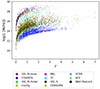 |
Fig. 1. Redshift-luminosity plot of the complete composite sample of radio AGN used in this work. The names of the fields are denoted in the legend. |
4. Bayesian modelling of luminosity functions
The LFs in this work were modelled within the Bayesian framework. The aim of Bayesian modelling is to determine the posterior P(Θ|D, M), or the probability density function, of the model parameters Θ, given D, M, which represent the data and model, respectively. The posterior is calculated using the prior π and the likelihood ℒ (Thrane & Talbot 2019):
 (1)
(1)
where E is the normalisation factor, also called the evidence:
 (2)
(2)
The likelihood function describes the measurements, and we discuss it in detail in the next subsection. The prior function quantifies our knowledge of the parameters before any measurements are taken (Thrane & Talbot 2019). In this work, the priors were chosen to be uniform, reflecting no prior assumptions about the model parameters. Priors for parameters expressed as logarithms were taken to be uniform in the logarithmic scale. In order to perform the numerical calculations, we used the “DYNESTY” programme package by Speagle (2020), which uses dynamic nested sampling (Skilling 2004; Higson et al. 2019).
4.1. Likelihood function
A crucial step in the process of Bayesian parameter estimation is determining the likelihood function. To do so, we followed Marshall et al. (1983, see also Christlein et al. 2009 for a more detailed derivation). By dividing the complete luminosity-redshift space into infinitesimal cells dzdL and assuming that each cell is small enough to contain up to one source, invoking the Poisson distribution, the probability of observing N sources of the complete sample is:
 (3)
(3)
where λ is the expected number of sources per bin. The first product goes over the complete sample of N sources, while the second one takes into account that all the remaining cells must remain empty. The expected density of sources in a given luminosity bin dL is given by the LF ϕ(z, L):
 (4)
(4)
By taking the customary logarithm of the probability and rearranging the sums, we obtain:
 (5)
(5)
where ϕi and Vi are associated with a particular source of the catalogue. The first sum goes over the observed sample. The second sum, which was turned into an integral, covers the whole available (z, L) space. The limits of the integral therefore follow the detection limit of the survey (i.e. it numbers all the cells where, in principle, a source could be observed). It therefore also follows that the integral equals the total predicted number of sources above the detection limit of the survey (Christlein et al. 2009). The log-likelihood, lnℒ, is defined as (e.g. Marshall et al. 1983):
 (6)
(6)
The expression can be further simplified by noting that not all terms depend on the LF parameters. The first term of the last equation can be divided into
 (7)
(7)
The second term of this relation does not depend on the LF parameters, and as such, it provides the lnL relation with a constant value not important in the minimisation process. It can therefore be omitted. We have finally
 (8)
(8)
This expression is the one found commonly in the literature (e.g. Kelly et al. 2008; Yuan et al. 2020). Furthermore, this expression can be generalised naturally to multiple fields j with different detection limits and observational areas as:
 (9)
(9)
where the first sum covers all the sources from all the composite fields and each integral in the second sum reaches the depth of the corresponding field as denoted by the lower limit. If the incompleteness of the survey near the detection limit is significant, it can be included as a separate completeness function, as described in the next subsection.
4.2. Completeness corrections
The completeness corrections of each survey can be introduced naturally by using a smooth detection limit, which is a function of flux, instead of an abrupt cut-off. The corrections for each survey were taken from their respective papers, as described below.
For the XXL-North field, the correction is given in XXL Paper XXIX. This correction corresponds to the one arising from noise near the detection limit. In XXL Paper XLI, we also introduced another correction arising from the losses during the matching of radio data with the multi-wavelength catalogue, which were not negligible. This correction is a function of redshift.
For the COSMOS field, the correction can be found in Smolčić et al. (2017b) in their Fig. 16 or Table 2. Finally, as seen from XXL Paper XVIII and Willott et al. (2001), the other catalogues can be considered complete. Therefore, for these catalogues, no corrections were included.
4.3. Model comparison
A feature of the Bayesian formalism discussed above is the ability to compare the fit between different models. A direct comparison is obtained by calculating the odds ratio (Thrane & Talbot 2019):
 (10)
(10)
where we have re-introduced the evidence from Sect. 4, E = p(D|M, I) (Liddle 2007). If, furthermore, there is no model preferred by the priors, the odds ratio reduces to a ratio of evidences called the Bayes factor:
 (11)
(11)
This ratio is also commonly expressed as a difference in log-scale. It should be noted that this method naturally selects models with a lower number of parameters, or in other words, it incorporates Occam’s razor (Liddle 2007).
Another more approximative method is the Akaike information criterion (AIC; Akaike 1974; Liddle 2007, XXL Paper VI). The definition of the AIC value is
 (12)
(12)
where k denotes the number of parameters. The model with the lower value of AIC is the one that corresponds to a better fit. It can be seen that this method also penalises a larger number of parameters. In other words, Occam’s razor is included naturally within the comparison.
Lastly, we have the Bayesian information criterion (BIC; Schwarz 1978; Liddle 2007, XXL Paper VI), which is similar to AIC and defined as
 (13)
(13)
where N is the number of data points. This value is the numerical approximation for the Bayes factor. From the above expression, it is also immediately clear that for a sufficiently large N, the BIC penalty for a large number of parameters is stronger than that of AIC.
5. Maximum volume method
A complementary non-parametric method to the Bayesian formalism is the method of maximum volumes described by Schmidt (1968, see also Felten 1976; Avni & Bahcall 1980; Page & Carrera 2000; Yuan & Wang 2013; Novak et al. 2017). This method naturally incorporates the inherent bias arising from detection limits of observations by taking into account that more luminous sources are detectable from farther away. The LF values in each luminosity and redshift bin are estimated by summing the inverse maximum volumes of possible observations for each source: 1/VMax, i. The error bars of the data points are estimated assuming Gaussian statistics (Marshall 1985; Boyle et al. 1988; Page & Carrera 2000; Novak et al. 2017), except when the number of sources equals less than ten. In those situations we used the values calculated by Gehrels (1986). Furthermore, the number of sources used here was an effective number determined from maximum volumes, as described in Ananna et al. (2022).
A further complication arose from the fact that we used multiple fields with varying depth. In order to coherently determine the value of the LF, we followed the procedure described in Avni & Bahcall (1980, see also Giallongo et al. 2005; Johnston 2011; Gruppioni et al. 2013; XXL Paper VI). The maximum volume for each source was calculated by taking into consideration all the fields where, in principle, this source could have been detected. For a given range of redshifts [z1, z2], we write
 (14)
(14)
Here, the sum goes over all the fields j where source i could have been observed, and ωj denotes the area of the respective field. The upper limit of the integral was the minimum between z2 and the maximum redshift of possible detection given the detection limit of the corresponding survey. In other words, we took into account that sources from the shallow fields are detectable in all the deeper fields as well, which modifies the value of their maximum volume (Gruppioni et al. 2013). In practice, the integral in the last equation was calculated numerically by dividing the redshift interval into smaller subsets, following the procedure described in XXL Paper XLI. The detection limits of each survey were shifted to 1400 MHz by assuming a power law and using the mean value of the spectral index.
6. Luminosity function models
One of the main aims of this work is to use the Bayesian framework to compare between different LF models. We list in this section all the different models used in this work. The complete list of models is also summarised in Table 2.
Luminosity function models used in this work, corresponding list of free parameters, and their number NPar.
6.1. Local luminosity function
The shape of the local LF is usually described by a power-law with an exponential cut-off (Saunders et al. 1990; Sadler et al. 2002; Smolčić et al. 2009):
![Mathematical equation: $$ \begin{aligned} \Phi _0(L) = \Phi ^* \left(\frac{L}{L^*}\right)^{1-\alpha } \exp \left\{ \frac{-1}{2\sigma ^2} \left[\log \left(1 + \frac{L}{L^*}\right)\right]^2\right\} , \end{aligned} $$](/articles/aa/full_html/2024/04/aa46947-23/aa46947-23-eq17.gif) (15)
(15)
where the base of the logarithm is ten. Here, L* is the break luminosity, Φ* is the normalisation, and σ is the high-luminosity slope. Another possible choice would have been the double power law often used for radio and X-ray AGN samples (Dunlop & Peacock 1990; Mauch & Sadler 2007; Smolčić et al. 2017a, XXL Paper VI). We discuss our choice in more detail in the discussion section. Lastly, another possibility is the bimodal model from Willott et al. (2001), which has a different form for the low- and high-luminosity ends of the sample. This model is discussed separately in Sect. 6.3.
6.2. Evolution
The evolution of the aforementioned local LFs is given by both density and luminosity evolution as (e.g. Smolčić et al. 2017a)
![Mathematical equation: $$ \begin{aligned} \Phi (L,z) = (1+z)^{\alpha _{\rm D}} \times \Phi _0 \left[\frac{L}{(1+z)^{\alpha _{\rm L}}}\right], \end{aligned} $$](/articles/aa/full_html/2024/04/aa46947-23/aa46947-23-eq18.gif) (16)
(16)
where αD and αL are the parameters quantifying density and luminosity evolution, respectively. In this work, we refer to this model as Sadler+02. We also tested pure density evolution (PDE) and pure luminosity evolution (PLE) where only one evolution parameter is different from zero. Another parametrisation of LF evolution can be found in Novak et al. (2017):
![Mathematical equation: $$ \begin{aligned} \Phi (L,z) = (1+z)^{(\alpha _{\rm D} + z \beta _{\rm D})} \times \Phi _0 \left[\frac{L}{(1+z)^{(\alpha _{\rm L} + z \beta _{\rm L})}}\right], \end{aligned} $$](/articles/aa/full_html/2024/04/aa46947-23/aa46947-23-eq19.gif) (17)
(17)
where β parameters quantify the change of evolution with redshift. We refer to this model as Novak+18. In order to account for the difference in evolution between the high- and low-luminosity ends of the sample, we also investigated the luminosity-dependent density evolution (LDDE; Schmidt & Green 1983; Ueda et al. 2003) following XXL Paper VI:
 (18)
(18)
where
 (19)
(19)
where La is the luminosity where the evolution changes according to the relation (19), zc is redshift after which the evolution changes, and p1, 2 represents the parameters of evolution. Lastly, as introduced by Massardi et al. (2010) and Bonato et al. (2017), the evolution of sources can be described by a luminosity-dependent luminosity evolution model (LDLE) where the break luminosity L* evolves as
![Mathematical equation: $$ \begin{aligned} L^*(z) = L^*(0) \cdot 10^{\left\{ k_{\rm evo} z \left[2z_{\rm top} - 2z^{m_{\rm ev}} z_{\rm top}^{1-m_{\rm ev}} / \left(1 + m_{\rm ev}\right) \right] \right\} } \end{aligned} $$](/articles/aa/full_html/2024/04/aa46947-23/aa46947-23-eq22.gif) (20)
(20)
and
 (21)
(21)
Here, kevo and mev are free parameters of evolution, while ztop, 0 and δztop determine the redshift where the evolution changes.
6.3. Bimodal luminosity function model
A special case for both the local LF and its evolution is the bimodal model taken from Willott et al. (2001). We refer to it in this work as Willott+01. The shape and evolution of the sample have a different analytical form for the high- and low-luminosity ends of the sample. Following Smolčić et al. (2009), in this work we used model C from Willott et al. (2001), it being the most flexible one, defined as
 (22)
(22)
where Φl is the low-luminosity end of the function,
 (23)
(23)
and Φh is the high-luminosity end,
![Mathematical equation: $$ \begin{aligned} {\Phi _{\rm h}} = {\left\{ \begin{array}{ll} {\Phi _{\rm h0} \left(\frac{L}{L_{\rm h}^*}\right)^{-\alpha _{\rm h}} \exp \left(\frac{L_{\rm h}^*}{-L}\right) \cdot \exp \left[\frac{-1}{2} \left(\frac{z - z_{\rm h0}}{z_{\rm h1}}\right)\right]},&{z < z_{\rm h0}}\\ {\Phi _{\rm h0} \left(\frac{L}{L_{\rm h}^*}\right)^{-\alpha _{\rm h}} \exp \left(\frac{L_{\rm h}^*}{-L}\right) \cdot \exp \left[\frac{-1}{2} \left(\frac{z - z_{\rm h0}}{z_{\rm h2}}\right)\right]},&{z > z_{\rm h0}} \end{array}\right.}. \end{aligned} $$](/articles/aa/full_html/2024/04/aa46947-23/aa46947-23-eq26.gif) (24)
(24)
Here, L* denotes the break luminosity, Φ0 is the normalisation, and α is the slope of the LFs. Parameter z0 is the redshift at which the evolution changes. These parameters exist separately for the high-and low-luminosity ends of the sample, as denoted by the extra indices h, l. Parameters kl, zh1, and zh2 quantify the evolution.
7. Results
7.1. Testing the methodology
Before using the observed data discussed in Sect. 2, we tested the methodology by using simulated data. For this purpose, we created custom Python codes that created catalogues of mock observations starting from an assumed LF. We then tried to re-create the assumed LF by modelling the LFs using our methodology on simulated mock observations. We tested both the parametric method described in Sect. 4 and the method of maximum volumes described in Sect. 5. The tests were performed for a wide range of different fields and their combinations, starting with a wide range of assumed LFs. The results were always in good agreement with the starting LF, within the range of the uncertainties defined via 90% quantiles for a sample of LFs drawn randomly from the posterior. This provided us with confidence that the methodology used in this work is sound.
As an example, we describe here the process performed on a Schechter LF model, with a superposition of PDE and PLE evolution (named Sadler+02 within this work). The area of the field was set to 40.46 deg2 and the detection limit to 50 μJy. This resulted in a simulated catalogue of 6378 mock sources above the detection limit, created by randomly selecting sources via the assumed LF. The starting parameters of the LF are given in Table 3. We set the scatter in redshifts to be negligible, but a finite uncertainty in redshifts, via hierarchical Bayesian interference, was also tested. The parameter modelling was performed on this simulated dataset using the same codes later used on observational data. The retrieved parameters are also shown in Table 3. The detection limit in this example was a step function (i.e. the completeness corrections were not present). We also assumed a mean spectral index of −0.7. The codes were also tested for non-negligible completeness corrections by introducing completeness correction as a separate function during the integration of log-likelihood. The methodology was tested for all the models described in Sect. 6 and on different areas and depths of mock-catalogues. The parameters of the LFs were always retrieved successfully.
Assumed and retrieved parameters resulting from the modelling of LFs on simulated data.
7.2. The luminosity functions using the COSMOS, XXL, 3CRR, 7C, 6CE, CENSORS, BRL, Wall & Peacock, and Config surveys
The same methods, which were successfully tested on simulations, were used on real observed data, namely, from the COSMOS, XXL, 3CRR, 7C, and 6CE fields as well as the CENSORS, BRL, Wall & Peacock, and Config surveys, described in Sect. 2. We combined all the catalogues into a single composite survey. We estimated the best model parameters for all LFs discussed in Sect. 6. The numerical calculations were performed by the DYNESTY programme package (Speagle 2020), which yielded both the model parameter posteriors and the marginal likelihoods for each model. We also obtained the posterior samples useful for plotting the LFs, as they preserved the correlation between the parameters of the model.
According to our data, the best-fitting model is the LDDE model of evolution with an exponential local form described by relations (15), (18) and (19). The relative standing of each fit was assessed by comparing their marginal likelihoods. Apart from this, we also used the approximate AIC and BIC methods introduced in Sect. 4.3. The resulting values of the model comparison are listed in Table 4. We show a comparison between the best-fitting LDDE model and all of the other models in the table. We list the values of three different methods: difference in logarithm of evidence, AIC, and BIC separately. The relative standing of the models remains the same across all three methods, with the LDDE model consistently as the preferred one. According to the Jeffreys’ interpretation of evidence ratios (e.g. Kass & Raftery 1995), the interpretation varies from “strong” (> 10) to “decisive” (> 100) in favour of the LDDE model.
Comparison of the LDDE model with other models using three different methods, as described in the text.
The LDDE model’s LFs are shown in Fig. 2 since this was the best-fitting model. The grey lines correspond to the median and the 90% quantiles and were obtained from a random sample of LFs drawn from the posterior. Apart from the Bayesian method, we also show the data points obtained from the maximum volume method described in Sect. 5. It can be seen that the two complementary methods give consistent results. Certain discrepancies between the methods can be seen in the last sub-plot of the figure, but at such high redshifts (z > 3), the number of sources is small, and the LF is less constrained, as visible by the number of sources for each data point given in Fig. 2.
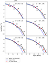 |
Fig. 2. Luminosity functions modelled using the COSMOS, XXL, 3CRR, 7C, 6CE, CENSORS, BRL, Wall & Peacock, and Config surveys and obtained by two complementary methods: Bayesian modelling and the method of maximum volumes. Grey lines denote the median and 90% quantiles of the parametric Bayesian inference. These values were obtained by randomly drawing samples from the posterior. The crosses denote the non-parametric method of maximum volumes along with the corresponding error bars. The uncertainties were derived assuming Poisson errors except when the number of sources was lower than ten. For such data points, the uncertainties were represented by tabulated errors determined by Gehrels (1986). Here, the number of sources was an effective number determined from maximum volumes, as described in Ananna et al. (2022). We also show the number of sources creating each data point. The blue dashed fiducial line denotes the LF determined in the first redshift bin. |
In Fig. 3, we show the resulting parameters of the LDDE model via a corner plot of the posterior probability density functions. The break luminosity equalled  and
and  . The degeneracy in p1 and p2 parameters is an expected occurrence, as seen from Eq. (18), but it was eliminated by choosing the prior so that it encompasses only one peak. The modelling was also tested without this simplification, and the results were qualitatively identical. The resulting values of the parameters determined from the posterior probability density functions are shown within Fig. 3 and listed within Table 5.
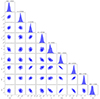 |
Fig. 3. Corner plot showing the posterior distribution of each parameter of the LDDE model. The resulting samples and weights taken from the posterior were further smoothed as described in Speagle (2020) to obtain the plotted probability density functions. |
Parameters of the best fitting LDDE model.
We also show in Fig. 4 the LFs created only via the non-parametric method of maximum volumes, as these data points trace the AGN sample directly, without any need of assumed models. The LFs for different redshift bins are shown overlaid together, so the evolution of AGN is clearly visible. The evolution is stronger for high-luminosity sources. The redshift bin with median redshift zMed = 3.38 was created using a lower number of sources, and the LF is therefore less constrained. The high redshift LF could also point towards a turnover in density at these redshifts, which is less clear from the modelled LFs. However, we note again that the models are not constrained well above z ≈ 3.
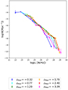 |
Fig. 4. Non-parametric LFs determined in different redshift bins via method of maximum volumes (Sect. 5) shown overlaid on top of each other in order to display their evolution. The uncertainties were derived assuming Poisson errors except when the effective number of sources, determined from maximum volumes as described in Ananna et al. (2022), was lower than ten. For such data points, the uncertainties were represented by tabulated errors determined by Gehrels (1986). The evolution is stronger for high-luminosity sources. The last redshift bin was created using a smaller sub-sample of sources and is, as described in the text, less credible. |
A comparison between the best-fitting LDDE model and the other non-optimal fits performed within this work is shown in Fig. 5. Furthermore, separate plots for each non-optimal fit are given as supplementary material in the appendix. As a means of further model comparison, in Fig. 6, we show the redshift distributions of sources from each survey compared to the model predictions. The model predictions were obtained by integrating the LF models, taking into account the detection limit of each survey and the corresponding incompleteness described in Sect. 4.2. The figure shows the model predictions for each LF model used within this work. It can be seen that the LDDE model is the one that is able to reproduce the redshift distributions best, particularly regarding the shallow fields of the large area where the other models failed to adequately reproduce the redshift distributions. This is a consequence of the fact that these models are not flexible enough to describe the “bump” present in the LFs at high luminosities.
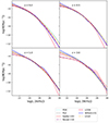 |
Fig. 5. Comparison between the best-fitting LDDE model and the other non-optimal fits. All fits were performed within this work on the same composite dataset. The shaded area for the LDDE model denotes the 90% quantiles of the parametric Bayesian inference obtained by randomly drawing samples from the posterior. The other models are represented by medians. |
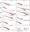 |
Fig. 6. Redshift distribution of sources shown as a number of sources divided by the width of the redshift bin. The figure shows both the observed redshift histograms as data points as well as the model prediction lines. The shaded areas are the 85% quantiles obtained by randomly drawing samples from the posterior. |
7.3. Comparison with the literature
The best-fitting LDDE model from this work was compared to a set of radio LF models from the literature, namely, Willott et al. (2001), McAlpine et al. (2013), Smolčić et al. (2017a), Ceraj et al. (2018), and Ocran et al. (2021). The survey from Willott et al. (2001) is already described in Sect. 2. The sample from McAlpine et al. (2013) contained 942 sources observed in the radio wavelength with the VLA. The sample from Smolčić et al. (2017a) contained 1800 AGN sources from the COSMOS field. Ceraj et al. (2018) LFs were also determined from the COSMOS field, with a sample of 1604 sources. The LFs by Ocran et al. (2021) were created from 486 AGN from the ELAIS N1 field observed at 610 MHz. Since the majority of the surveys modelled the LFs with pure PDE or PLE evolution, we show a comparison on two different plots in Fig. 7, one for each type of evolution, in order to make them more intelligible. The surveys used in the comparison are listed in the legend. Both plots also show the model from Willott et al. (2001), with the parameters taken from the corresponding paper, as it is neither a PDE nor a PLE model. As seen from the plots, our results are broadly consistent with earlier surveys, although our comparison based on Bayesian evidence comparison shows the LDDE model to be the preferred model (see Table 4). Almost none of the surveys, except (Willott et al. 2001), feature the bump at higher luminosities present in our results. The model from Willott et al. (2001) shows a difference in evolution as a function of luminosity, but the exact shape of the LFs differs somewhat from our model. There is also a difference in the model from Willott et al. (2001) with other models at lower luminosities, but this is a result of their sample not being able to constrain these values well, as discussed in their paper. This is because the sample from Willott et al. (2001) contains 356 sources mostly from only the higher luminosity set of our sample. Since our whole sample uses a composite set of surveys, our results are not affected by this.
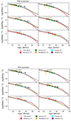 |
Fig. 7. Comparison of our LDDE model with the models from the literature, shown separately for PDE and PLE literature evolution models, as denoted above the figures. The used surveys are denoted in the legend. We also show the maximum volume data points taken from the literature in the same colour as the corresponding LF model line. The results of this work, represented by 90% quantiles are given in pink. The Willott LF shown is the one derived by Willott et al. (2001). |
7.4. Additional checks
In order to test the robustness of our results, a few additional checks were performed. Firstly, we examined the effect of spectral indices on the results. To assess this, we re-modelled the LFs using different values of spectral indices: a mean value of −0.7 for all sources and a mean value of the corresponding field for each source. The quantitative results remained consistent. Secondly, we assessed the redshift uncertainties of the XXL-N field, this being the field with the largest uncertainties in redshift. This could have been done using the hierarchical Bayes method (see Loredo 2004; Aird et al. 2010, XXL Paper VI). However, since the fields of intermediate depth in this work are already represented by the XXL-S field, a conservative check was performed by simply omitting the XXL-N field. The re-modelling of the LFs again gave consistent results, proving the uncertainties in the redshifts of the XXL-N field do not modify our results. Lastly, we note that the same ranking between the evolution models was obtained by using the double power law function of Dunlop & Peacock (1990) for the local shape of the LF. The results of the model selection overall seem to be a true consequence of the physical processes within AGN and not a result of unforeseen biases and point towards the LDDE model being the best one.
7.5. Effect of spectral indices on the model parameters
The luminosities of the sources and the flux re-calculation from different frequencies depend on the value of the spectral indices. However, not all of the sources used in the LF modelling had a determined spectral index. As already noted, for the missing indices, we used the mean spectral index of the corresponding survey. This did not take into account the frequency or redshift dependence of the spectral indices (e.g. Tisanić et al. 2020). In order to assess the effect of the spectral index on the parameters of the best-fitting LDDE model, we performed the model parameter estimation again using only the sources with a determined spectral index at first and then assuming a mean spectral index of −0.7 for all sources. The results remained consistent, with the LDDE model being determined as the best one. The newly determined model parameters are listed in Tables 6 and 7.
Parameters of the best-fitting LDDE model for modelling using only the determined values of spectral indices.
Parameters of the best fitting LDDE model for modelling using a mean value of spectral index set to −0.7.
7.6. Number and luminosity density
Using the best-fitting LDDE model, we estimated the number density and the luminosity density of sources as a function of redshift. The number density of sources was calculated as:
 (25)
(25)
where the luminosity range was chosen as log[LMin, LMax]/(W/Hz) = [22, 30]. The luminosity density was calculated within the same luminosity range as
 (26)
(26)
The densities are shown in Figs. 8 and 9, extrapolated up to a redshift of z = 6 in order to compare them with the high-redshift quasar studies. We used the estimation of the quasar LF at z = 6 from Gloudemans et al. (2021) and calculated the densities via relations (25) and (26). Their LF was estimated by combining the properties of radio quasars at z = 2 with the UV-LF at z = 6, assuming that the fraction of radio-loud quasars remains constant from z = 2 to z = 6, as described in detail in Gloudemans et al. (2021). Since the LF from Gloudemans et al. (2021) spans a smaller luminosity range, the number density should be considered a lower limit. This effect, however, is not so important when calculating the luminosity density, as the integrated function is weighted by the value of the luminosity. Another comparison was made with the high-redshift LF of quasars from Saxena et al. (2017), predicted by the model developed within their work. The semi-analytical model uses black hole mass functions and the Eddington ratio distribution, taking into account the energy losses due to synchrotron, adiabatic, and inverse Compton processes, in order to predict the radio LF. The model also includes radio jets with powers determined via black hole mass and Eddington ratios. The radio LF was compared to observational data at z = 2, providing satisfactory results, and then extended to z = 6. The details of the model are described in detail in their work. The LFs resulting from the model were again integrated via relations (25) and (26) to obtain the densities.
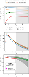 |
Fig. 8. Number density. Upper panel: number density calculated at 1.4 GHz for a set of different luminosity ranges of the same width, as denoted in the legend above the figure. The black dots represent the maximum value of each line. Middle panel: number density at 1.4 GHz calculated for a set of progressively increasing luminosity ranges, as denoted in the legend above the figure. Lower panel: number density at 1.4 GHz as a function of redshift for a set of different surveys, denoted in the legend. The data points denote the high-redshift quasar surveys as described in the text. The uncertainties in this work are calculated from the resulting samples within the parametric Bayesian method as 90% quantiles. The uncertainties of the literature values were determined as maximum uncertainties of the parameters, as described in the text. The shaded area in the plots denote a higher redshift where the LF models are less constrained. The high-redshift quasar density from Gloudemans et al. (2021) is a lower limit, as the luminosity range of the LF used in the calculation was smaller. |
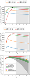 |
Fig. 9. Luminosity density. Upper panel: luminosity density at 1.4 GHz calculated for a set of different luminosity ranges of the same width, as denoted in the legend above the figure. The black dots represent the maximum value of each line. Middle panel: luminosity density at 1.4 GHz calculated for a set of progressively increasing luminosity ranges, as denoted in the legend above the figure. Lower panel: luminosity density at 1.4 GHz as a function of redshift for a set of different surveys, denoted in the legend. The data points denote the high-redshift quasar surveys, as described in the text. The uncertainties in the figure follow those in Fig. 8. The shaded area in the plots denote a higher redshift where the LF models are less constrained. |
We also show the number and luminosity densities obtained from LF models of Ceraj et al. (2018) and Smolčić et al. (2017a). Although, as described in these papers, the LFs do not reach such high redshifts, we extrapolated them to z = 6 in order to compare them with the high-redshift quasar surveys. The models assume that the evolution changes with redshift analogously with the model by Novak et al. (2017) described in relation (17). The uncertainties plotted in the figure are the maximum between the 1σ uncertainties in parameters α and β. At lower redshifts, the results are consistent, with differences arising at high redshifts (of z ≈ 5). This is due to the different LF models used to describe the data. A slight difference in number density at low redshifts is the consequence of slightly different normalisation of the local LF.
An interesting aspect of the luminosity density is the flattening at high redshifts. This effect is due to the bump present in the LDDE model at the high-luminosity end of the sample. To further illustrate this, in Figs. 8 and 9, we also plot the number and luminosity density using different luminosity ranges, each spanning progressively higher luminosities. Since the flattening occurs only when the upper luminosity boundary is high, we concluded that the high-luminosity sources responsible for the bump in the LF model are responsible for the flattening of the luminosity density. The maximum values of these functions also change with luminosity bins. For a luminosity density at 1.4 GHz, these values equal
![Mathematical equation: $$ \begin{aligned}&z = 0.39 \pm 0.05, \ \ \ \log L \in [22,24] \end{aligned} $$](/articles/aa/full_html/2024/04/aa46947-23/aa46947-23-eq34.gif) (27)
(27)
![Mathematical equation: $$ \begin{aligned}&z = 0.60 \pm 0.03, \ \ \ \log L \in [24,26] \end{aligned} $$](/articles/aa/full_html/2024/04/aa46947-23/aa46947-23-eq35.gif) (28)
(28)
![Mathematical equation: $$ \begin{aligned}&z = 1.98 \pm 0.2, \ \ \ \log L \in [26,28] \end{aligned} $$](/articles/aa/full_html/2024/04/aa46947-23/aa46947-23-eq36.gif) (29)
(29)
![Mathematical equation: $$ \begin{aligned}&z = 2.51 \pm 0.06, \ \ \ \log L \in [28,30]. \end{aligned} $$](/articles/aa/full_html/2024/04/aa46947-23/aa46947-23-eq37.gif) (30)
(30)
The values were estimated by taking the mean value from five random samples of the posterior.
7.7. Stellar mass dependent difference in evolution
In order to assess the dependence of the LF evolution on stellar mass, we divided our sample into two sub-populations of high- and low-mass galaxies. Since the XXL-N survey contained no stellar mass estimates, we excluded it from these considerations. We reasoned that the intermediate surveys are already constrained by the XXL-S field, so this simplification is not crucial. The stellar mass estimates for the COSMOS field come from the COSMOS2015 catalogue (Laigle et al. 2016) and were calculated from spectra as described in Laigle et al. (2016). The XXL-S field stellar mass estimates were determined by SED fitting as described in XXL Paper XXXI. The fields from Willott et al. (2001) lacked stellar mass estimates but contained apparent K-band magnitudes, via a publicly available catalogue1. The complete publicly available catalogue, for all three shallow fields, 7C, 6CE, and 3CRR, contained 181 sources. The 7C had complete K-band magnitudes at z > 1.2, so a threshold was imposed on this dataset and a correction was made during the calculation of likelihood. The 3CRR field had 69/96 sources with K-band magnitudes at z > 0.05. This incompleteness was incorporated via a correction function to the likelihood function. The 6CE field had complete K-band magnitude data. The details on the catalogues can be found in Willott et al. (2003). In order to estimate the stellar masses, we used the relationship between the stellar mass of the galaxy and its K-band magnitude reported in the literature (e.g. Arnouts et al. 2007). Since we were dealing with a sub-population composed purely of AGN, we re-calibrated the stellar mass to K-band correlation. For this, we used the COSMOS2015 catalogue that contains both of these values. We took a subset of the catalogue containing only AGN based on radio excess, as previously described in Sect. 3, and we re-plotted the dependence of stellar mass on the absolute K-band magnitude, as shown in Fig. 10. Following Arnouts et al. (2007), we allowed for a redshift-dependent correlation via two free redshift-dependent parameters as log(M*) = a(z)K + b(z). We first performed a linear regression fit on every redshift subset independently. The resulting parameters a and b differed across redshift bins. By performing another linear regression on these values, we assessed the redshift dependence of the parameters. The resulting correlation parameters thus equalled
 (31)
(31)
 (32)
(32)
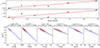 |
Fig. 10. Calibration of mass-to-light correlation between the absolute K-band magnitude and stellar mass obtained from the COSMOS2015 catalogue for the subset of AGN sources. The assumed functional form of the correlation is M* = a(z)K + b(z), as described in the text. Bottom: dependence of stellar mass M* on K-band magnitude. The blue line shows the linear regression fit performed for each redshift bin independently. The range of each redshift bin as well as the resulting correlation parameters are given above the corresponding plot. Top: resulting correlation parameters as a function of redshift. The red line shows the linear regression performed on these values to determine the redshift dependence of the parameters. |
Furthermore, to eliminate any systematic error arising from the incompleteness of our sample due to a finite detection limit, we removed the lowest-mass galaxies from our sample. The two stellar mass sub-populations therefore spanned mass intervals of log(M*)∈[10.2, 11] and log(M*) > 11, ranging in log-luminosities for both subsets from ≈22 to ≈28. The difference in evolution can be seen in Fig. 11. We modelled the evolution as a simple PDE evolution since we were interested only in tracing the difference between the sub-populations. The difference in evolution exists and is larger than the 68.2 quantiles plotted in the figure. The parameter of the PDE evolution (see Eq. (16)) equalled  for the low-mass sample and
  for the high-mass sample, but the differences of the functions arose also as a result of the complete LF shape. As a final precaution, we repeated the LF fitting without the 7C survey since this survey had the largest incompleteness. The results remained qualitatively the same. All in all, the difference in LFs could point towards some kind of bimodality within our AGN sample that is a function of host galaxy stellar mass. The details of this bimodality, however, need to be investigated further.
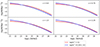 |
Fig. 11. Luminosity functions for the high and low mass sub-sample. The uncertainty plotted in the figure is the 68.2 quantile. The model of evolution is the PDE model. The redshift of each sub-plot is given in the figure. |
7.8. Source counts
Using the shape of the modelled LFs, it is possible to construct the AGN source counts of our sample. We show in Fig. 12 the AGN source counts obtained from our model of the LF when drawing 500 parameter samples from the posterior. From the definition of the LF Φ(L, z), the number of sources ΔN in each flux bin at a certain value of redshift was obtained as
 (33)
(33)
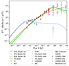 |
Fig. 12. Source counts modelled together with data points obtained directly from the catalogues. The green dashed line denotes the model obtained from LFs constrained within this work. The errors were determined by selecting 500 samples from the posterior. The red, blue, and black lines denote models from Novak et al. (2018) obtained from LFs for AGN, SFGs, and the total population, respectively. The data points represent the source counts obtained from the catalogues as denoted in the legend. The catalogues are the same as described in Sect. 2 except for the ones denoted as Vernstrom+14, which were taken from another study by Vernstrom et al. (2014). The COSMOS SFGs are sources from the COSMOS catalogue not selected by the radio excess threshold described in Sect. 2. The outlier data points are due to the finite detection limit. |
where dV/dz is the differential co-moving volume, Δlog L is the luminosity decade, and dz is the redshift bin. The number of sources obtained in each flux bin was summed over all redshift bins and then normalised with counts expected in a static Euclidean Universe. For comparison, we also show source counts from an earlier study by Vernstrom et al. (2014) and the model obtained from the LF evolutionary model by Novak et al. (2018), as this is the model constrained by the deeper COSMOS survey, and as such, it constrains the low-luminosity end of the sample the best. The source counts by Vernstrom et al. (2014) were obtained from 3 GHz data of the Karl G. Jansky Very Large Array when directed towards the Lockman Hole. The source counts were constructed using the probability of deflection method to reach deeper values of flux, as described in Vernstrom et al. (2014). The model by Novak et al. (2018) was constructed from the LFs that have pure luminosity evolution with different parameters for SFGs and the AGN population, as described in detail in that paper.
8. Discussion
We modelled the LFs via the Bayesian parametric method and a composite sample consisting of multiple surveys of varying area and depth (z < 3 and log L ∈ [22, 29]) that together span a large interval in both redshift and luminosity. We compared a set of LF models and concluded that by all used criteria, the LDDE model is preferred. This result is broadly consistent with earlier studies where the difference in evolution was observed between sub-samples of high and low luminosity.
8.1. Evolution of AGN sub-populations in the literature
The difference in the evolution of the high- and low-luminosity ends of the sample is reported throughout the literature (Hook et al. 1998; Waddington et al. 2001; Willott et al. 2001; Clewley & Jarvis 2004; Sadler et al. 2007; Smolčić et al. 2009; Donoso et al. 2009; Padovani et al. 2017). There are, however, differences in the adopted LF models. As already stated, Willott et al. (2001) used a bimodal model where the shape and evolution of the high-and low-luminosity ends have a different functional form. Smolčić et al. (2009) only modelled the low end of the AGN sample using a superposition of luminosity and density evolution, analogous to relation (16), and showed a modest evolution of this sample compared to the high-luminosity studies. Furthermore, studies are often performed via non-parametric methods (e.g. Waddington et al. 2001; Sadler et al. 2007; Donoso et al. 2009; Rigby et al. 2015), so no functional form is assumed for the LF. Even so, there is a difference in evolution that seems to be a function of luminosity, which makes these results consistent with our work.
A difference in evolution between two subsets of AGN was observed in a study by Pracy et al. (2016) using the Faint Images of the Radio Sky at Twenty centimeters survey matched with the Sloan Digital Sky Survey. The complete AGN sample was divided into HERGs and LERGs based on optical spectra. There was an observed difference in evolution in the double power-law LF assuming alternatively both PDE or PLE evolution where the LERG population evolved slowly, in contrast to the more rapid evolution of the HERG sub-sample. Though the comparison is not exact, due to a difference in classification, this difference in evolution is consistent with our results, where the evolution depends on luminosity.
Padovani et al. (2015) divided their Extended Chandra Deep Field-South Very Large Array sample into RQ and RL AGN based on the relative strength of radio emission at 1.4 GHz, as described in the text, where RL sources correspond to the ones with radio excess2. The RL AGN correspond mostly to jet-mode AGN, and RQ AGN correspond to radiative-mode AGN. A difference in evolution between these two sub-populations was observed: the RL sample exhibited a peak at z = 0.5, after which their numbers declined, in contrast to the RQ sample. These findings are also consistent with this work.
A study by Ocran et al. (2021) of the ELAIS N1 field observed with the GMRT at 610 MHz divided the complete sample into RQ and RL AGN based on a combination of multi-wavelength criteria as described in their text. The evolution was modelled as PLE for the sub-samples, and a difference in evolution was observed where RL AGN evolved more strongly. This is again consistent with our results.
Similar conclusions concerning AGN evolution have also been obtained within X-ray astronomy. An example is the study by XXL Paper VI, which used a composite set of fields, including MAXI, HBSS, XMM-COSMOS, Lockman Hole, XMM-CDFS, AEGIS-XD, Chandra-COSMOS, and Chandra-CDFS. The LFs were modelled using an AGN sample observed within the X-ray part of the spectrum in the 5 − 10 keV band. The model comparison was also done within the Bayesian framework, comparing AIC and BIC and resulting in LDDE being the best-fitting model.
On the other hand, some studies, such as Yuan et al. (2016), argue via theoretical arguments against the LDDE model, explaining the phenomenology within the framework of luminosity and density evolution mixture model. This is not consistent with our results.
8.2. The existence of two AGN sub-populations
A trend throughout the literature is the separation of the full AGN sample into sub-samples, be it based on RL and RQ, the relative strength of the radio emission (e.g. Padovani et al. 2015), high HERG and LERG, optical spectral lines (XXL Paper XXXVI), flat and steep spectrum sources, the spectral index (Wall 1975; Massardi et al. 2010; Bonato et al. 2017), or any other criterion. Although the LDDE model (preferred in this work) assumes a continuous change in evolution with regards to luminosity, this does not exclude the existence of two sub-populations. Firstly, the strength of the model selection criteria between the model from Willott et al. (2001) and LDDE is not as strong compared to the simple PDE and LDE models, and the difference could be a consequence of the larger number of parameters of the Willott model. More importantly, if the sub-populations are not selected with a simple luminosity threshold, a different fraction of each population can be present at different luminosities. This could lead to the observed continuous change in evolution with luminosity present in the LDDE model. Concentrating on the underlying physical processes, these results are therefore still consistent with the picture outlined in the introduction, where there exist two distinct modes of accretion: the radiatively efficient mode and the radiatively inefficient mode (Hardcastle et al. 2007; Heckman & Best 2014; Narayan et al. 1998; Shakura & Sunyaev 1973). Although the analogies are not exact, the radiatively efficient mode would correspond to the high-luminosity end, or the HERG sub-sample, while the inefficient mode would correspond to the low-luminosity end, or the LERG sub-sample.
8.3. Kinetic luminosity
Apart from the observed radio emission, a large part of the energy stored in the AGN jets is given to the environment kinetically via work performed by jet expansion (e.g. Smolčić et al. 2017a). In order to assess this power and to gain insight into how the feedback of AGN evolves through cosmic time, we investigated the kinetic luminosity of our sample. Using the correlation from Ceraj et al. (2018, see also Smolčić et al. 2017a), we determined the kinetic luminosity from the radio luminosity following the relation
 (34)
(34)
where f was introduced by Willott et al. (1999) in order to incorporate all the possible systematic errors and was determined to be in the range 1 − 20. Following Ceraj et al. (2018), we set it to 15. It should be noted, however, that the parameter changes the luminosity by a multiplicative constant factor. The corresponding kinetic luminosity density will therefore shift systematically on the y-axis, but the shape of the redshift dependence will remain the same. The uncertainties are also large enough to include the star-forming component of radio emission. We calculated the kinetic luminosity density as a function of redshift:
 (35)
(35)
Here, we again used the samples from the LDDE model as described in the last subsection. The resulting plot is shown in Fig. 13. Apart from our observational results, we also show the estimated kinetic luminosity density obtained from the GALFORM model (Fanidakis et al. 2012) and the SAGE model (Croton et al. 2006). The GALFORM model assumes two different modes of black hole accretion and subsequently two different evolution modes through cosmic time. The first mode is the starburst mode where accretion arises from galaxy mergers or instabilities within the disc. The second mode is the hot-halo mode where matter from the hot halo accretes onto the central black hole. An interesting aspect of the GALFORM model is the flattening between the observed kinetic luminosity and the total and starburst modes of the GALFORM model at redshifts z ≈ 3 − 4, not present in the SAGE model. The SAGE model, which includes the feedback mechanism, has the black hole accretion rate ṁ as one of its results. Following Croton et al. (2016) and Ceraj et al. (2018), we calculated the kinetic luminosity from this value as 0.1 · ṁ · c2, multiplying this by 0.08, which was the radio mode efficiency parameter. The factor 0.1 is the standard value found in the literature, falling between the efficiency expected for a non-spinning and maximally spinning black hole (Croton et al. 2016). Our comparison with the SAGE model gave non-consistent results. Even if we ignore the absolute values of the functional forms, which can be explained with the uncertainty factor f given in relation (34), the shape (i.e. redshift dependence) is different between the model and the observations. Furthermore, Fig. 13 shows that the two models give different kinetic luminosity estimates. The differences between the models and between our observational results are probably due to the assumptions made in the models.
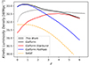 |
Fig. 13. Kinetic luminosity density as a function of redshift (in grey). The uncertainties were calculated from the resulting samples of the parametric method as 90% quantiles. The black, red, and blue lines correspond to the predictions from GALFORM. The black line is the total density, while the red and blue lines denote the hot-halo and starburst modes, respectively. The orange dashed line represents the SAGE model. |
8.4. Downsizing and feedback
The described trend of different evolution and cut-offs can be explained via cosmic downsizing, where the more massive black holes form earlier than the less massive ones (e.g. Rigby et al. 2015). This trend is, at first glance, not consistent with the hierarchical model, where larger black holes are the product of merging, but the apparent inconsistency can be explained by a switch in the mode of accretion from efficient cold gas accretion to inefficient hot gas accretion via a process called feedback, where inefficient accretion starts to dominate at low redshifts (e.g. Heckman & Best 2014; Rigby et al. 2015). In other words, the accretion onto the central black hole is a complex process where the rate of accretion can lead to a feedback effect, slowing it down or even quenching it. Consequently, there is a switch between the high-efficiency accretion to low-efficiency accretion. This, in turn, affects the properties of AGN through cosmic time and hence the AGN evolution. Since we argue for a luminosity-dependent evolution of AGN in this work, it is consistent with a physical picture requiring feedback. In short, the difference in evolution as a function of AGN luminosity shows that the physics of AGN evolution depends on the accretion rate. This is consistent with the picture of AGN accretion that incorporates feedback. This also places our results in line with other publications where feedback was either deduced indirectly via scaling relations of the host galaxy and its black hole (Magorrian et al. 1998; Ferrarese & Merritt 2000; Gebhardt et al. 2000; Graham et al. 2011; Sani et al. 2011; Beifiori et al. 2012; McConnell & Ma 2013) or observed more directly via galactic winds (e.g. Nesvadba et al. 2008; Feruglio et al. 2010; Veilleux et al. 2013; Tombesi et al. 2015) or X-ray cavities in galactic groups and clusters (Clarke et al. 1997; Rafferty et al. 2006; McNamara & Nulsen 2007; Fabian 2012; Nawaz et al. 2014; Kolokythas et al. 2015). Lastly, the need for AGN feedback is also supported by simulations (Fanidakis et al. 2012; Hirschmann et al. 2012; Croton et al. 2016; Harrison et al. 2018).
9. Summary and conclusion
We modelled the radio LFs of AGN using a composite survey of varying area and depth. The composite survey was comprised of the COSMOS, XXL-North, XXL-South, 7C, 6CE, 3CRR, CENSORS, BRL, Wall & Peacock, and Config fields and contained 5446 sources. This allowed us to constrain the LFs at both high redshifts (up to z ≈ 3) and at high luminosities (log L ∈ [22, 29]). The functions were modelled with an emphasis on the parametric method within the Bayesian framework, which allowed us to select the best-fitting model from a set of different shapes and evolutions. The best-fitting model according to marginal likelihood comparison, as well as the AIC and BIC methods, is the LDDE model, Using the Jeffreys’ interpretation, evidence ratios varied from “strong” (> 10) to “decisive” (> 100). The parameter posteriors were determined from the Bayesian model fitting, and the resulting values were determined as listed in Table 5. The dependence of the shape and evolution of the LFs on luminosity assumed by this model was discussed in its implications on the physical picture of AGN evolution through cosmic time. Although the change in evolution as a function of luminosity is continuous, this does not exclude the possibility of AGN sub-populations as being different fractions of each sub-population that can be found at different luminosities. We discussed the number density and luminosity density as a function of redshift. The shape of the best-fitting LDDE model resulted in a flattening at higher redshifts that is not present in simpler models with pure density or luminosity evolution. We compared these results with high-redshift quasar surveys and found broad consistency. We calculated the kinetic luminosity density and compared it to model-estimated values, finding some consistency with the GALFORM simulation but not with the SAGE model. Furthermore, in order to assess the dependence of the stellar-mass of host galaxies on AGN evolution, we divided our sample into subsets of different stellar mass and modelled the evolution using a simpler PDE model. The difference in LFs that we observed was larger than the 65% quantiles estimated from posterior samples. Taken together, all these results point to a physical picture of AGN evolution where a simple density evolution, luminosity evolution, or a superposition of both is not enough to trace the details of AGN evolution. More complex models, either consisting of AGN sub-populations or including a dependence on AGN luminosity, are needed.
The classification of RL and RQ sources is not consistent throughout the literature. See Padovani et al. (2017), Sect. 2.1.3. for details.
Acknowledgments
We thank the anonymous referee for insightful comments that improved the quality of the paper. V.S. acknowledges the European Union’s Seventh Framework programme under grant agreement 337595 (CoSMass). B.S. and V.S. acknowledge the financial support by the Croatian Science Foundation for project IP-2018-01-2889 (LowFreqCRO). Z.I. acknowledges support by the US Fulbright Scholar Program and hospitality at the Ruđer Boković Institute, Zagreb, Croatia. XXL is an international project based around an XMM Very Large Programme surveying two 25 deg2 extragalactic fields at a depth of ∼6 × 10⁻¹⁵ erg cm−2 s−1 in the [0.5 − 2] keV band for point-like sources. The XXL website is http://irfu.cea.fr/xxl. Multi-band information and spectroscopic follow-up of the X-ray sources are obtained through a number of survey programs, summarised at http://xxlmultiwave.pbworks.com/. M.P. acknowledges long-term support from the Centre National d’Études Spatiales (CNES).
References
- Aird, J., Nandra, K., Laird, E. S., et al. 2010, MNRAS, 401, 2531 [Google Scholar]
- Akaike, H. 1974, IEEE Trans. Autom. Control, 19, 716 [Google Scholar]
- Ananna, T. T., Weigel, A. K., Trakhtenbrot, B., et al. 2022, ApJS, 261, 9 [NASA ADS] [CrossRef] [Google Scholar]
- Arnouts, S., Walcher, C. J., Le Fèvre, O., et al. 2007, A&A, 476, 137 [CrossRef] [EDP Sciences] [Google Scholar]
- Avni, Y., & Bahcall, J. N. 1980, ApJ, 235, 694 [NASA ADS] [CrossRef] [Google Scholar]
- Beifiori, A., Courteau, S., Corsini, E. M., & Zhu, Y. 2012, MNRAS, 419, 2497 [NASA ADS] [CrossRef] [Google Scholar]
- Best, P. N., Röttgering, H. J. A., & Lehnert, M. D. 1999, MNRAS, 310, 223 [NASA ADS] [CrossRef] [Google Scholar]
- Best, P. N., Röttgering, H. J. A., & Lehnert, M. D. 2000, MNRAS, 315, 21 [NASA ADS] [CrossRef] [Google Scholar]
- Best, P. N., Arts, J. N., Röttgering, H. J. A., et al. 2003, MNRAS, 346, 627 [Google Scholar]
- Bock, D. C. J., Large, M. I., & Sadler, E. M. 1999, AJ, 117, 1578 [Google Scholar]
- Bonato, M., Negrello, M., Mancuso, C., et al. 2017, MNRAS, 469, 1912 [Google Scholar]
- Boyle, B. J., Shanks, T., & Peterson, B. A. 1988, MNRAS, 235, 935 [NASA ADS] [Google Scholar]
- Brookes, M. H., Best, P. N., Peacock, J. A., Röttgering, H. J. A., & Dunlop, J. S. 2008, MNRAS, 385, 1297 [NASA ADS] [CrossRef] [Google Scholar]
- Butler, A., Huynh, M., Delhaize, J., et al. 2018a, A&A, 620, A3 [NASA ADS] [CrossRef] [EDP Sciences] [Google Scholar]
- Butler, A., Huynh, M., Delvecchio, I., et al. 2018b, A&A, 620, A16 [NASA ADS] [CrossRef] [EDP Sciences] [Google Scholar]
- Butler, A., Huynh, M., Kapińska, A., et al. 2019, A&A, 625, A111 [NASA ADS] [CrossRef] [EDP Sciences] [Google Scholar]
- Ceraj, L., Smolčić, V., Delvecchio, I., et al. 2018, A&A, 620, A192 [NASA ADS] [CrossRef] [EDP Sciences] [Google Scholar]
- Christlein, D., Gawiser, E., Marchesini, D., & Padilla, N. 2009, MNRAS, 400, 429 [NASA ADS] [CrossRef] [Google Scholar]
- Ciliegi, P., Jurlin, N., Butler, A., et al. 2018, A&A, 620, A11 [Google Scholar]
- Clarke, D. A., Harris, D. E., & Carilli, C. L. 1997, MNRAS, 284, 981 [CrossRef] [Google Scholar]
- Clewley, L., & Jarvis, M. J. 2004, MNRAS, 352, 909 [NASA ADS] [CrossRef] [Google Scholar]
- Condon, J. J., Cotton, W. D., Greisen, E. W., et al. 1998, AJ, 115, 1693 [Google Scholar]
- Croton, D. J., Springel, V., White, S. D. M., et al. 2006, MNRAS, 365, 11 [Google Scholar]
- Croton, D. J., Stevens, A. R. H., Tonini, C., et al. 2016, ApJS, 222, 22 [Google Scholar]
- Delvecchio, I., Smolčić, V., Zamorani, G., et al. 2017, A&A, 602, A3 [NASA ADS] [CrossRef] [EDP Sciences] [Google Scholar]
- Donoso, E., Best, P. N., & Kauffmann, G. 2009, MNRAS, 392, 617 [Google Scholar]
- Dunlop, J. S., & Peacock, J. A. 1990, MNRAS, 247, 19 [NASA ADS] [Google Scholar]
- Fabian, A. C. 2012, ARA&A, 50, 455 [Google Scholar]
- Fanidakis, N., Baugh, C. M., Benson, A. J., et al. 2012, MNRAS, 419, 2797 [NASA ADS] [CrossRef] [Google Scholar]
- Felten, J. E. 1976, ApJ, 207, 700 [NASA ADS] [CrossRef] [Google Scholar]
- Ferrarese, L., & Merritt, D. 2000, ApJ, 539, L9 [Google Scholar]
- Feruglio, C., Maiolino, R., Piconcelli, E., et al. 2010, A&A, 518, L155 [NASA ADS] [CrossRef] [EDP Sciences] [Google Scholar]
- Fotopoulou, S., Pacaud, F., Paltani, S., et al. 2016, A&A, 592, A5 [NASA ADS] [CrossRef] [EDP Sciences] [Google Scholar]
- Gebhardt, K., Bender, R., Bower, G., et al. 2000, ApJ, 539, L13 [Google Scholar]
- Gehrels, N. 1986, ApJ, 303, 336 [Google Scholar]
- Gendre, M. A., & Wall, J. V. 2008, MNRAS, 390, 819 [NASA ADS] [Google Scholar]
- Giallongo, E., Salimbeni, S., Menci, N., et al. 2005, ApJ, 622, 116 [CrossRef] [Google Scholar]
- Gloudemans, A. J., Duncan, K. J., Röttgering, H. J. A., et al. 2021, A&A, 656, A137 [NASA ADS] [CrossRef] [EDP Sciences] [Google Scholar]
- Graham, A. W., Onken, C. A., Athanassoula, E., & Combes, F. 2011, MNRAS, 412, 2211 [NASA ADS] [CrossRef] [Google Scholar]
- Gruppioni, C., Pozzi, F., Rodighiero, G., et al. 2013, MNRAS, 432, 23 [Google Scholar]
- Hardcastle, M. J., Evans, D. A., & Croston, J. H. 2007, MNRAS, 376, 1849 [NASA ADS] [CrossRef] [Google Scholar]
- Harrison, C. M., Costa, T., Tadhunter, C. N., et al. 2018, Nat. Astron., 2, 198 [Google Scholar]
- Heckman, T. M., & Best, P. N. 2014, ARA&A, 52, 589 [Google Scholar]
- Higson, E., Handley, W., Hobson, M., & Lasenby, A. 2019, Stat. Comput., 29, 891 [Google Scholar]
- Hirschmann, M., Somerville, R. S., Naab, T., & Burkert, A. 2012, MNRAS, 426, 237 [NASA ADS] [CrossRef] [Google Scholar]
- Hook, I. M., Shaver, P. A., & McMahon, R. G. 1998, ASP Conf. Ser., 146, 17 [NASA ADS] [Google Scholar]
- Johnston, R. 2011, A&ARv, 19, 41 [NASA ADS] [CrossRef] [Google Scholar]
- Kass, R. E., & Raftery, A. E. 1995, J. Am. Stat. Assoc., 90, 773 [Google Scholar]
- Kelly, B. C., Fan, X., & Vestergaard, M. 2008, ApJ, 682, 874 [NASA ADS] [CrossRef] [Google Scholar]
- Kolokythas, K., O’Sullivan, E., Giacintucci, S., et al. 2015, MNRAS, 450, 1732 [NASA ADS] [CrossRef] [Google Scholar]
- Lacy, M., Rawlings, S., Hill, G. J., et al. 1999, MNRAS, 308, 1096 [NASA ADS] [CrossRef] [Google Scholar]
- Laigle, C., McCracken, H. J., Ilbert, O., et al. 2016, ApJS, 224, 24 [Google Scholar]
- Liddle, A. R. 2007, MNRAS, 377, L74 [NASA ADS] [Google Scholar]
- Loredo, T. J. 2004, AIP Conf. Ser., 735, 195 [NASA ADS] [CrossRef] [Google Scholar]
- Magorrian, J., Tremaine, S., Richstone, D., et al. 1998, AJ, 115, 2285 [Google Scholar]
- Marshall, H. L. 1985, ApJ, 299, 109 [NASA ADS] [CrossRef] [Google Scholar]
- Marshall, H. L., Tananbaum, H., Avni, Y., & Zamorani, G. 1983, ApJ, 269, 35 [NASA ADS] [CrossRef] [Google Scholar]
- Massardi, M., Bonaldi, A., Negrello, M., et al. 2010, MNRAS, 404, 532 [NASA ADS] [Google Scholar]
- Mauch, T., & Sadler, E. M. 2007, MNRAS, 375, 931 [Google Scholar]
- McAlpine, K., Jarvis, M. J., & Bonfield, D. G. 2013, MNRAS, 436, 1084 [CrossRef] [Google Scholar]
- McConnell, N. J., & Ma, C.-P. 2013, ApJ, 764, 184 [Google Scholar]
- McNamara, B. R., & Nulsen, P. E. J. 2007, ARA&A, 45, 117 [NASA ADS] [CrossRef] [Google Scholar]
- Narayan, R., Mahadevan, R., Grindlay, J. E., Popham, R. G., & Gammie, C. 1998, ApJ, 492, 554 [Google Scholar]
- Nawaz, M. A., Wagner, A. Y., Bicknell, G. V., Sutherland, R. S., & McNamara, B. R. 2014, MNRAS, 444, 1600 [NASA ADS] [CrossRef] [Google Scholar]
- Nesvadba, N. P. H., Lehnert, M. D., De Breuck, C., Gilbert, A. M., & van Breugel, W. 2008, A&A, 491, 407 [NASA ADS] [CrossRef] [EDP Sciences] [Google Scholar]
- Novak, M., Smolčić, V., Delhaize, J., et al. 2017, A&A, 602, A5 [NASA ADS] [CrossRef] [EDP Sciences] [Google Scholar]
- Novak, M., Smolčić, V., Schinnerer, E., et al. 2018, A&A, 614, A47 [NASA ADS] [CrossRef] [EDP Sciences] [Google Scholar]
- Ocran, E. F., Taylor, A. R., Vaccari, M., et al. 2021, MNRAS, 500, 4685 [Google Scholar]
- Padovani, P., Bonzini, M., Kellermann, K. I., et al. 2015, MNRAS, 452, 1263 [Google Scholar]
- Padovani, P., Alexander, D. M., Assef, R. J., et al. 2017, A&ARv, 25, 2 [Google Scholar]
- Page, M. J., & Carrera, F. J. 2000, MNRAS, 311, 433 [Google Scholar]
- Pracy, M. B., Ching, J. H. Y., Sadler, E. M., et al. 2016, MNRAS, 460, 2 [Google Scholar]
- Rafferty, D. A., McNamara, B. R., Nulsen, P. E. J., & Wise, M. W. 2006, ApJ, 652, 216 [NASA ADS] [CrossRef] [Google Scholar]
- Rawlings, S., Eales, S., & Lacy, M. 2001, MNRAS, 322, 523 [NASA ADS] [CrossRef] [Google Scholar]
- Rigby, E. E., Argyle, J., Best, P. N., Rosario, D., & Röttgering, H. J. A. 2015, A&A, 581, A96 [NASA ADS] [CrossRef] [EDP Sciences] [Google Scholar]
- Sadler, E. M., Jackson, C. A., Cannon, R. D., et al. 2002, MNRAS, 329, 227 [Google Scholar]
- Sadler, E. M., Cannon, R. D., Mauch, T., et al. 2007, MNRAS, 381, 211 [NASA ADS] [CrossRef] [Google Scholar]
- Sani, E., Marconi, A., Hunt, L. K., & Risaliti, G. 2011, MNRAS, 413, 1479 [NASA ADS] [CrossRef] [Google Scholar]
- Saunders, W., Rowan-Robinson, M., Lawrence, A., et al. 1990, MNRAS, 242, 318 [Google Scholar]
- Saxena, A., Röttgering, H. J. A., & Rigby, E. E. 2017, MNRAS, 469, 4083 [Google Scholar]
- Schinnerer, E., Sargent, M. T., Bondi, M., et al. 2010, ApJS, 188, 384 [Google Scholar]
- Schmidt, M. 1968, ApJ, 151, 393 [Google Scholar]
- Schmidt, M., & Green, R. F. 1983, ApJ, 269, 352 [NASA ADS] [CrossRef] [Google Scholar]
- Schwarz, G. 1978, Ann. Stat., 6, 461 [Google Scholar]
- Shakura, N. I., & Sunyaev, R. A. 1973, A&A, 24, 337 [NASA ADS] [Google Scholar]
- Skilling, J. 2004, AIP Conf. Ser., 735, 395 [Google Scholar]
- Šlaus, B., Smolčić, V., Novak, M., et al. 2020, A&A, 638, A46 [NASA ADS] [CrossRef] [EDP Sciences] [Google Scholar]
- Smolčić, V., Zamorani, G., Schinnerer, E., et al. 2009, ApJ, 696, 24 [CrossRef] [Google Scholar]
- Smolčić, V., Novak, M., Delvecchio, I., et al. 2017a, A&A, 602, A6 [NASA ADS] [CrossRef] [EDP Sciences] [Google Scholar]
- Smolčić, V., Novak, M., Bondi, M., et al. 2017b, A&A, 602, A1 [Google Scholar]
- Smolčić, V., Delvecchio, I., Zamorani, G., et al. 2017c, A&A, 602, A2 [NASA ADS] [CrossRef] [EDP Sciences] [Google Scholar]
- Smolčić, V., Intema, H., Šlaus, B., et al. 2018, A&A, 620, A14 [NASA ADS] [CrossRef] [EDP Sciences] [Google Scholar]
- Speagle, J. S. 2020, MNRAS, 493, 3132 [Google Scholar]
- Tasse, C., Röttgering, H. J. A., Best, P. N., et al. 2007, A&A, 471, 1105 [NASA ADS] [CrossRef] [EDP Sciences] [Google Scholar]
- Thrane, E., & Talbot, C. 2019, PASA, 36, e010 [NASA ADS] [CrossRef] [Google Scholar]
- Tisanić, K., Smolčić, V., Imbrišak, M., et al. 2020, A&A, 643, A51 [NASA ADS] [CrossRef] [EDP Sciences] [Google Scholar]
- Tombesi, F., Meléndez, M., Veilleux, S., et al. 2015, Nature, 519, 436 [NASA ADS] [CrossRef] [Google Scholar]
- Ueda, Y., Akiyama, M., Ohta, K., & Miyaji, T. 2003, ApJ, 598, 886 [NASA ADS] [CrossRef] [Google Scholar]
- Veilleux, S., Meléndez, M., Sturm, E., et al. 2013, ApJ, 776, 27 [Google Scholar]
- Vernstrom, T., Scott, D., Wall, J. V., et al. 2014, MNRAS, 440, 2791 [CrossRef] [Google Scholar]
- Waddington, I., Dunlop, J. S., Peacock, J. A., & Windhorst, R. A. 2001, MNRAS, 328, 882 [NASA ADS] [CrossRef] [Google Scholar]
- Wall, J. V. 1975, The Observatory, 95, 196 [NASA ADS] [Google Scholar]
- Wall, J. V., & Peacock, J. A. 1985, MNRAS, 216, 173 [NASA ADS] [CrossRef] [Google Scholar]
- Willott, C. J., Rawlings, S., Blundell, K. M., & Lacy, M. 1999, MNRAS, 309, 1017 [Google Scholar]
- Willott, C. J., Rawlings, S., Blundell, K. M., Lacy, M., & Eales, S. A. 2001, MNRAS, 322, 536 [NASA ADS] [CrossRef] [Google Scholar]
- Willott, C. J., Rawlings, S., Jarvis, M. J., & Blundell, K. M. 2003, MNRAS, 339, 173 [Google Scholar]
- Yuan, Z., & Wang, J. 2013, Ap&SS, 345, 305 [NASA ADS] [CrossRef] [Google Scholar]
- Yuan, Z., Wang, J., Zhou, M., & Mao, J. 2016, ApJ, 820, 65 [NASA ADS] [CrossRef] [Google Scholar]
- Yuan, Z., Jarvis, M. J., & Wang, J. 2020, ApJS, 248, 1 [NASA ADS] [CrossRef] [Google Scholar]
Appendix A: Stellar mass catalogue description
The columns of the catalogue of stellar masses, introduced in Sect. 7.7 (available at the CDS, see main-title footnote), are as follows:
-
Name: Name of the radio source.
-
z: Best available redshift for the source.
-
S_1400_MHz: Source flux at 1400 MHz in mJy.
-
Alpha: Spectral index of the source. Set to the mean of respective field when not available.
-
Mstar: Stellar mass of the source. Determined as described in Sect. 7.7.
-
Survey: Name of original survey from where the source was taken. "C" denotes COSMOS, "XXL-N" and "XXL-S" denote the North and South XXL fields, "3" denotes the 3CRR field, "6" refers to the 6CE field, and "7" denotes the 7C field.
This catalogue is a compilation from other surveys, except for the stellar masses of the 3CRR, 7C, and 6CE surveys. These were determined from magnitudes within this work, as described in the text.
Appendix B: Non-optimal model fits
As described in Sect. 7, the best-fitting model according to all selection criteria was the LDDE model (see Tab. 4) described by relations (18) and (19). The LDDE model LFs fit is shown in Fig. 2. For completeness, we show the LF fits for all the other models described in Sect. 6 that were deemed a less optimal fit than the LDDE model. In Figs. B.1 to B.6, we show the models along the data points obtained by using the maximum volume method. All the fits were performed on the same composite survey dataset described in Sect. 2. The LF plots were created in the same manner as in Fig. 2.
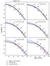 |
Fig. B.1. Sadler+02 model LF fit. The model evolution is described in relation (16). The notation follows Fig. 2. |
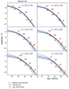 |
Fig. B.4. Novak+18 model LF fit. The model evolution is described in relation (17). The notation follows Fig. 2. |
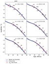 |
Fig. B.6. LDLE model LF fit. The model evolution is described in relations (20) and (21). The notation follows Fig. 2. |
All Tables
Luminosity function models used in this work, corresponding list of free parameters, and their number NPar.
Assumed and retrieved parameters resulting from the modelling of LFs on simulated data.
Comparison of the LDDE model with other models using three different methods, as described in the text.
Parameters of the best-fitting LDDE model for modelling using only the determined values of spectral indices.
Parameters of the best fitting LDDE model for modelling using a mean value of spectral index set to −0.7.
All Figures
|
Fig. 1. Redshift-luminosity plot of the complete composite sample of radio AGN used in this work. The names of the fields are denoted in the legend. |
| In the text | |
|
Fig. 2. Luminosity functions modelled using the COSMOS, XXL, 3CRR, 7C, 6CE, CENSORS, BRL, Wall & Peacock, and Config surveys and obtained by two complementary methods: Bayesian modelling and the method of maximum volumes. Grey lines denote the median and 90% quantiles of the parametric Bayesian inference. These values were obtained by randomly drawing samples from the posterior. The crosses denote the non-parametric method of maximum volumes along with the corresponding error bars. The uncertainties were derived assuming Poisson errors except when the number of sources was lower than ten. For such data points, the uncertainties were represented by tabulated errors determined by Gehrels (1986). Here, the number of sources was an effective number determined from maximum volumes, as described in Ananna et al. (2022). We also show the number of sources creating each data point. The blue dashed fiducial line denotes the LF determined in the first redshift bin. |
| In the text | |
|
Fig. 3. Corner plot showing the posterior distribution of each parameter of the LDDE model. The resulting samples and weights taken from the posterior were further smoothed as described in Speagle (2020) to obtain the plotted probability density functions. |
| In the text | |
|
Fig. 4. Non-parametric LFs determined in different redshift bins via method of maximum volumes (Sect. 5) shown overlaid on top of each other in order to display their evolution. The uncertainties were derived assuming Poisson errors except when the effective number of sources, determined from maximum volumes as described in Ananna et al. (2022), was lower than ten. For such data points, the uncertainties were represented by tabulated errors determined by Gehrels (1986). The evolution is stronger for high-luminosity sources. The last redshift bin was created using a smaller sub-sample of sources and is, as described in the text, less credible. |
| In the text | |
|
Fig. 5. Comparison between the best-fitting LDDE model and the other non-optimal fits. All fits were performed within this work on the same composite dataset. The shaded area for the LDDE model denotes the 90% quantiles of the parametric Bayesian inference obtained by randomly drawing samples from the posterior. The other models are represented by medians. |
| In the text | |
|
Fig. 6. Redshift distribution of sources shown as a number of sources divided by the width of the redshift bin. The figure shows both the observed redshift histograms as data points as well as the model prediction lines. The shaded areas are the 85% quantiles obtained by randomly drawing samples from the posterior. |
| In the text | |
|
Fig. 7. Comparison of our LDDE model with the models from the literature, shown separately for PDE and PLE literature evolution models, as denoted above the figures. The used surveys are denoted in the legend. We also show the maximum volume data points taken from the literature in the same colour as the corresponding LF model line. The results of this work, represented by 90% quantiles are given in pink. The Willott LF shown is the one derived by Willott et al. (2001). |
| In the text | |
|
Fig. 8. Number density. Upper panel: number density calculated at 1.4 GHz for a set of different luminosity ranges of the same width, as denoted in the legend above the figure. The black dots represent the maximum value of each line. Middle panel: number density at 1.4 GHz calculated for a set of progressively increasing luminosity ranges, as denoted in the legend above the figure. Lower panel: number density at 1.4 GHz as a function of redshift for a set of different surveys, denoted in the legend. The data points denote the high-redshift quasar surveys as described in the text. The uncertainties in this work are calculated from the resulting samples within the parametric Bayesian method as 90% quantiles. The uncertainties of the literature values were determined as maximum uncertainties of the parameters, as described in the text. The shaded area in the plots denote a higher redshift where the LF models are less constrained. The high-redshift quasar density from Gloudemans et al. (2021) is a lower limit, as the luminosity range of the LF used in the calculation was smaller. |
| In the text | |
|
Fig. 9. Luminosity density. Upper panel: luminosity density at 1.4 GHz calculated for a set of different luminosity ranges of the same width, as denoted in the legend above the figure. The black dots represent the maximum value of each line. Middle panel: luminosity density at 1.4 GHz calculated for a set of progressively increasing luminosity ranges, as denoted in the legend above the figure. Lower panel: luminosity density at 1.4 GHz as a function of redshift for a set of different surveys, denoted in the legend. The data points denote the high-redshift quasar surveys, as described in the text. The uncertainties in the figure follow those in Fig. 8. The shaded area in the plots denote a higher redshift where the LF models are less constrained. |
| In the text | |
|
Fig. 10. Calibration of mass-to-light correlation between the absolute K-band magnitude and stellar mass obtained from the COSMOS2015 catalogue for the subset of AGN sources. The assumed functional form of the correlation is M* = a(z)K + b(z), as described in the text. Bottom: dependence of stellar mass M* on K-band magnitude. The blue line shows the linear regression fit performed for each redshift bin independently. The range of each redshift bin as well as the resulting correlation parameters are given above the corresponding plot. Top: resulting correlation parameters as a function of redshift. The red line shows the linear regression performed on these values to determine the redshift dependence of the parameters. |
| In the text | |
|
Fig. 11. Luminosity functions for the high and low mass sub-sample. The uncertainty plotted in the figure is the 68.2 quantile. The model of evolution is the PDE model. The redshift of each sub-plot is given in the figure. |
| In the text | |
|
Fig. 12. Source counts modelled together with data points obtained directly from the catalogues. The green dashed line denotes the model obtained from LFs constrained within this work. The errors were determined by selecting 500 samples from the posterior. The red, blue, and black lines denote models from Novak et al. (2018) obtained from LFs for AGN, SFGs, and the total population, respectively. The data points represent the source counts obtained from the catalogues as denoted in the legend. The catalogues are the same as described in Sect. 2 except for the ones denoted as Vernstrom+14, which were taken from another study by Vernstrom et al. (2014). The COSMOS SFGs are sources from the COSMOS catalogue not selected by the radio excess threshold described in Sect. 2. The outlier data points are due to the finite detection limit. |
| In the text | |
|
Fig. 13. Kinetic luminosity density as a function of redshift (in grey). The uncertainties were calculated from the resulting samples of the parametric method as 90% quantiles. The black, red, and blue lines correspond to the predictions from GALFORM. The black line is the total density, while the red and blue lines denote the hot-halo and starburst modes, respectively. The orange dashed line represents the SAGE model. |
| In the text | |
|
Fig. B.1. Sadler+02 model LF fit. The model evolution is described in relation (16). The notation follows Fig. 2. |
| In the text | |
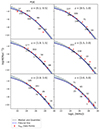 |
Fig. B.2. PDE model LF fit. The notation follows Fig. 2. |
| In the text | |
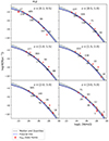 |
Fig. B.3. PLE model LF fit. The notation follows Fig. 2. |
| In the text | |
|
Fig. B.4. Novak+18 model LF fit. The model evolution is described in relation (17). The notation follows Fig. 2. |
| In the text | |
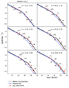 |
Fig. B.5. Willott+01 model LF fit. The model is described in Sect. 6.3. The notation follows Fig. 2. |
| In the text | |
|
Fig. B.6. LDLE model LF fit. The model evolution is described in relations (20) and (21). The notation follows Fig. 2. |
| In the text | |
Current usage metrics show cumulative count of Article Views (full-text article views including HTML views, PDF and ePub downloads, according to the available data) and Abstracts Views on Vision4Press platform.
Data correspond to usage on the plateform after 2015. The current usage metrics is available 48-96 hours after online publication and is updated daily on week days.
Initial download of the metrics may take a while.