| Issue |
A&A
Volume 697, May 2025
|
|
|---|---|---|
| Article Number | A69 | |
| Number of page(s) | 18 | |
| Section | Extragalactic astronomy | |
| DOI | https://doi.org/10.1051/0004-6361/202452912 | |
| Published online | 14 May 2025 | |
Mapping reionization bubbles in JWST era
I. Empirical edge detection with Lyman alpha emission from galaxies
1
Cosmic Dawn Center (DAWN), Copenhagen N, Denmark
2
Niels Bohr Institute, University of Copenhagen, Jagtvej 128, 2200 Copenhagen N, Denmark
3
Scuola Normale Superiore, Piazza dei Cavalieri 7, I-56126 Pisa, Italy
4
Scuola Internazionale Superiore di Studi Avanzati (SISSA), Via Bonomea 265, 34136 Trieste, Italy
5
Steward Observatory, University of Arizona, 933 N Cherry Ave, Tucson, AZ 85721, USA
6
Research School of Astronomy and Astrophysics, Australian National University, Canberra, ACT 2611, Australia
⋆ Corresponding author.
Received:
6
November
2024
Accepted:
21
March
2025
Abstract
Context. Ionized bubble sizes during reionization trace physical properties of the first galaxies. JWST's ability to spectroscopically confirm and measure Lyman-alpha (Lyα) emission in sub-L★ galaxies makes it possible to map to map ionized bubbles in 3D. However, existing Lyα-based bubble measurement strategies rely on constraints from single galaxies, which are limited by the large variability in intrinsic Lyα emission.
Aims. As a first step, we present two bubble-size-estimation methods using Lyα spectroscopy of ensembles of galaxies, enabling us to map ionized structures and marginalize over Lyα emission variability. We tested our methods using gigaparsec-scale reionization simulations of the intergalactic medium (IGM).
Methods. To map bubbles in the plane of the sky, we developed an edge detection method based on the asymmetry of Lyα transmission as a function of spatial position. To map bubbles along the line of sight, we develop an algorithm using the tight relation between Lyα transmission and the line-of-sight distance from galaxies to the nearest neutral IGM patch.
Results. Both methods can robustly recover bubbles with a radius ≳10 comoving Mpc, sufficient for mapping bubbles even in the early phases of reionization, when the IGM is ∼70−90% neutral. These methods require ≳0.002−0.004 galaxies/cMpc3, a 5σ Lyα equivalent width upper limit of ≲30 Å for the faintest targets, and redshift precision Δz≲0.015, which is feasible with JWST spectroscopy. Shallower observations will provide robust lower limits on bubble sizes. Additional constraints on IGM transmission from Lyα escape fractions and line profiles will further refine these methods, paving the way to our first direct understanding of ionized bubble growth.
Key words: intergalactic medium / dark ages, reionization, first stars
© The Authors 2025
 Open Access article, published by EDP Sciences, under the terms of the Creative Commons Attribution License (https://creativecommons.org/licenses/by/4.0), which permits unrestricted use, distribution, and reproduction in any medium, provided the original work is properly cited.
This article is published in open access under the Subscribe to Open model. This email address is being protected from spambots. You need JavaScript enabled to view it. to support open access publication.
1. Introduction
Between 20≳z≳5, the first luminous sources reionized neutral hydrogen in the intergalactic medium (IGM), forming ionized bubbles around them which eventually merged (e.g., see Mesinger et al. 2016, for a recent review). Understanding the properties, formation, and evolution of these first sources and how they drove the reionization process is a frontier in astronomy. While significant progress has been made in the last two decades in measuring the volumn-averaged timeline of reionization (e.g., Fan et al. 2006; Stark et al. 2010; Treu et al. 2012; Pentericci et al. 2014; Mason et al. 2018a; Davies et al. 2018; Jung et al. 2020; Qin et al. 2021; Bosman et al. 2022; Bolan et al. 2022; Umeda et al. 2024; Nakane et al. 2024; Tang et al. 2024a), we currently have no robust measurements of the typical sizes of ionized bubbles and how they evolve over time.
The first large bubbles are predicted to form around early galaxy overdensities, thus the sizes of ionized regions and their host overdensities can provide key insights into the reionization process. In individual regions this would enable ionizing photon “accounting”, where visible galaxies’ ionizing photon output can be compared to that required to grow the bubble, providing insight into their ionizing photon escape fractions and star formation histories, and the contribution of galaxies below even JWST's detection limits (e.g., Shapiro & Giroux 1987; Haiman 2002; Mason & Gronke 2020; Endsley & Stark 2022; Whitler et al. 2024; Torralba-Torregrosa et al. 2024). On a global scale, the distribution of ionized region sizes at a fixed redshift – the reionization “morphology” – is sensitive to the halo mass scale of the dominant ionizing sources (e.g., McQuinn et al. 2007a; Mesinger et al. 2016; Seiler et al. 2019; Hutter et al. 2023; Lu et al. 2024), with models where low-mass halos (Mh∼108 M⊙) dominate the ionizing-photon-budget-predicting median bubble radii of ∼10−30 cMpc (∼4−12 arcmin) during the mid-stages of reionization. In the next decade, there will be substantial observational efforts to identify and start characterizing the sizes of ionized regions over scales large enough to capture multiple bubbles, via upcoming 21 cm experiments to observe the neutral hydrogen directly (e.g., Yatawatta et al. 2013; Bowman et al. 2013) and wide-area near-IR spectroscopic surveys to observe galaxies that should trace ionized regions, for example, with Euclid, Roman, Subaru/Prime Focus Spectrograph (PFS), and Very Large Telescope (VLT)/Multi Object Optical and Near-infrared Spectrograph (MOONS) (van Mierlo et al. 2022; Euclid Collaboration: Scaramella et al. 2022; Wang et al. 2022; Greene et al. 2022; Maiolino et al. 2020; Gagnon-Hartman et al. 2025; Mesinger et al. 2024).
Lyman-alpha (Lyα) absorption by neutral hydrogen in high-z objects, such as galaxies, quasars (QSOs), and gamma-ray bursts, is currently our best tool to identify ionized regions, as Lyα suffers strong damping wing absorption due to neutral hydrogen in the foreground of the objects (Miralda-Escude & Rees 1998; Mesinger & Furlanetto 2008). Although considerably fainter than QSOs, galaxies have the benefit of being more numerous and less biased tracers of the reionization morphology (Shen et al. 2007; Eilers et al. 2024), such that they can be used to sample the IGM. Spectroscopic and narrow-band surveys in the last decades have identified a number of fields showing an excess of Lyα emission from galaxies at z∼6−9, implying large-scale (R>1 pMpc) ionized regions (e.g., Castellano et al. 2016; Tilvi et al. 2020; Endsley & Stark 2022; Wold et al. 2022; Napolitano et al. 2024; Tang et al. 2024a). Upcoming wide-area near-IR spectroscopy with Euclid, Roman, PFS, and MOONS will be able to identify more candidate ionized regions by detecting bright (≳1×10⁻¹⁷ erg s−1 cm−2) Lyα emission, and photometric overdensities of UV-bright galaxies. However, as we subsequently demonstrate, these instruments neither have the sensitivity to sample nor the wavelength coverage to spectroscopically confirm sufficient numbers of galaxies in these ionized regions to fully map bubbles and characterize their sizes (Hutter et al. 2018; Zackrisson et al. 2020), thus deeper follow-up imaging and spectroscopy will be required.
JWST has provided unique capabilities to make mapping these ionized regions, and the overdensities they surround, feasible. Its ability to spectroscopically confirm UV faint z>6 galaxies, even down to MUV≈−18 at z∼14 (Curtis-Lake et al. 2023; Carniani et al. 2024), has allowed us to precisely map z>5 galaxy distributions in 3D for the first time (e.g., Helton et al. 2024; Meyer et al. 2024; Chen et al. 2024; Tang et al. 2024a; Witstok et al. 2024). The sensitivity of NIRSpec (Jakobsen et al. 2022) has enabled the detection Lyα emission from UV-faint galaxies (e.g., Saxena et al. 2023; Tang et al. 2023; Chen et al. 2024; Jones et al. 2025), which is infeasible from the ground, and can be used to comprehensively trace ionized regions. JWST's ability to measure Lyα escape fractions from Balmer lines also provides a promising new indicator of highly ionized regions, where the fraction of Lyα escaping from galaxies through the IGM can reach close to unity (e.g., Chen et al. 2024). Such power makes it possible to map ionized bubbles. This potential has been demonstrated empirically in early JWST results. For example, the CEERS/EGS field, which contains ≳50% of all Lyα emission known to date above z>7, is likely the largest known ionized region at this epoch (Oesch et al. 2015; Roberts-Borsani et al. 2016; Stark et al. 2017; Tilvi et al. 2020; Jung et al. 2022; Larson et al. 2022). Several studies using NIRSpec spectroscopy have detected new high equivalent width (EW ≳ 100 Å) Lyα emission, and measured Lyα escape fractions to confirm several galaxies in the region likely transmit >50% of their Lyα through the IGM (Tang et al. 2023, 2024a; Jung et al. 2024; Napolitano et al. 2024; Chen et al. 2024). Chen et al. (2024) and Tang et al. (2024a) demonstrate z∼7−8 galaxies in EGS appear clustered in several narrow redshift bins around Lyα emitting galaxies, hinting at several proper-megaparsec-scale bubbles along the line of sight (LOS).
However, a quantitative link from discrete galaxy observations such as these to the sizes of ionized regions has so far been challenging due to the intrinsic variability of Lyα emission. With an estimate of the fraction of Lyα transmitted through the IGM, it should be possible to infer the LOS distance of a galaxy to neutral gas (e.g., Mesinger & Furlanetto 2008; Mason & Gronke 2020), providing we can estimate the Lyα emitted by the source, before attenuation by the IGM. In the past few years, significant progress has been made in understanding the properties of Lyα emerging from post-reionization (5≲z≲6) galaxies (e.g., Prieto-Lyon et al. 2023; Tang et al. 2024b; Bolan et al. 2024; Lin et al. 2024). In particular, JWST observations provide key information about the relations between galaxies’ Lyα emission (rest-frame equivalent widths, Lyα escape fractions fesc, Lyα, and Lyα velocity offsets and line-profiles) and galaxy UV and optical properties such as UV continuum magnitude, UV slopes and [OIII]+Hβ emission (e.g., Saxena et al. 2023, 2024; Prieto-Lyon et al. 2023; Chen et al. 2024; Tang et al. 2024b; Lin et al. 2024). These observations can be used as baselines to infer the impact of the neutral IGM on Lyα during reionization. However, even in the ionized IGM, Lyα properties such as EW, escape fraction and lineshape can vary by orders of magnitude in galaxies with similar physical properties (e.g., Stark et al. 2010; Oyarzún et al. 2017; Jaskot et al. 2019; Hayes et al. 2023), which radiative transfer simulations predict is largely due to sightline variability in neutral gas and dust distributions in the ISM and CGM (e.g., Smith et al. 2017; Blaizot et al. 2023).
The first attempts to infer the sizes of ionized regions have focused on individual galaxies, using the approach described above to infer the relation between Lyα transmission and the distance of the galaxy to the neutral IGM (e.g., Mason & Gronke 2020; Hayes & Scarlata 2023; Umeda et al. 2024; Witstok et al. 2024; Torralba-Torregrosa et al. 2024). However, the intrinsic variability of Lyα emission makes estimates of the sizes of ionized bubbles based on single galaxies highly uncertain. To provide robust estimates of the sizes of ionized regions thus requires combining information from ensembles of galaxies to overcome this variability.
In this work, we thus aim to provide simple approaches to map ionized bubbles using observations of ensembles of galaxies, given the new capabilities of JWST. Here we focus on empirical methods for detecting bubble edges via integrated Lyα observations (i.e. EW, escape fractions). In a companion paper, Nikolić et al. (2025), we will present a framework for inferring the centers and radii of individual ionized regions based on Lyα line profiles. In Section 2 we introduce our IGM simulations and forward modeling of Lyα emission. We develop methods to map ionized bubbles on the plane of the sky (Section 3) and along sightline skewers (Section 4) using galaxy Lyα emission observations, and describe the observational requirements for robust bubble size recovery. Our methods make use of the almost one-to-one relation between the IGM damping wing absorption profile and the distance of galaxies to the nearest neutral IGM. In Section 5, we discuss prospect for ionized bubble mapping with current and future facilities and surveys. We present our conclusions in Section 6.
Throughout this paper, we use a flat ΛCDM cosmology with Ωm = 0.31, ΩΛ = 0.69, and h = 0.68 and magnitudes are in the AB system.
2. IGM simulations and forward modeling galaxy observables
We create simulations of the IGM with forward-modeled galaxy observables to test our bubble mapping methods. In this section, we describe how we simulate ionization cubes (Section 2.1), model emitted Lyα lines from galaxies (Section 2.2) and infer the fraction of Lyα flux transmitted through the IGM for each galaxy (Section 2.3), which is the key input to our bubble mapping methods.
2.1. IGM simulations
We use 21cmFASTv21 (Mesinger et al. 2011, 2016; Sobacchi & Mesinger 2014) to create realistic, large volume reionization IGM simulations. 21cmFASTv2 is a semi-numerical code that can quickly create reionization simulations for coeval density cubes (Mesinger et al. 2011).
We create a (300 cMpc)3 density cube with (1.5 cMpc)3 resolution, smaller than the characteristic bubble size (≳10 cMpc) when IGM neutral fraction is <90% (Lu et al. 2024). We generate ionization cubes of  at z = 8 by changing the ionization efficiency of galaxies, similar to the approach described by Lu et al. (2024). For simplicity, we use a bright-galaxy-driven reionization model, in which Mh>1011 M⊙ halos can ionize the IGM. The broad bubble size distribution of our bright-galaxy-driven reionization model allows us to test bubble size recovery for a wide range of bubble size. We find our results do not depend significantly on
  (which is the dominant driver of bubble sizes) because our methods primarily rely on the change of IGM transmission at the edges of bubbles. Thus we also do not expect our results to change significantly if we had assumed another reionization model, which will change the characteristic bubble size. Moreover, since most of the IGM during reionization has only two phases, bubble edges remain equally distinct in most reionization models.
We extract a catalog of halo masses and positions at z = 8 from the density cube using extended Press-Schechter theory (Sheth et al. 2001) and a halo-filtering method developed by Mesinger & Furlanetto (2007). The minimum halo mass extracted in this work is ∼4.2×10⁹ M⊙. As described in Lu et al. (2024), we use the UV luminosity – halo mass relation from Mason et al. (2015, 2023), adding a scatter of 0.5 mag following Ren et al. (2018), Whitler et al. (2020), to map from halo masses to UV magnitude. Lu et al. (2024) demonstrated this reproduces the observed UV LFs very well at z∼7−10, though at the faint end (MUV≳−18) of LF in our simulation slightly underpredicts the number density of galaxies. In later sections we will investigate bubble mapping given different galaxy number densities by setting different MUV detection limits for mock observations with our simulations. When discussing the corresponding detection limits in real observations, we will quote MUV limits which match our simulated number densities using the LFs in Bouwens et al. (2021).
2.2. Forward modeling Lyα emission
We will use galaxies’ Lyα emission properties to recover transmissions at their positions in a bubble. To obtain these properties, we forward model the observed Lya emission lines following the approach by Mason et al. (2018a). We assume the intrinsic Lyα line shape is a single Gaussian, and model the observed line after transfer through interstellar medium (ISM), circumgalactic medium (CGM), and IGM.
We generate the Lyα damping wing optical depth due to the IGM for every halo (selecting ∼105 halos with MUV≤−17, or Mh≳109.6 M⊙) along a sightline in the +z-direction from the galaxy to a distance of 200 cMpc away2, using periodic boundary conditions. We calculate the Lyα damping wing optical depth profile, τIGM(ΔvLyα) (e.g., Miralda-Escude 1998) at Lyα velocity offsets from systemic (ΔvLyα) between −300 km/s and 5700 km/s by summing the contributions of LOS neutral hydrogen in the ionization cube as described in Mesinger et al. (2015).
Our Gaussian Lyα emission line model is described by two quantities: the velocity offset from systemic (ΔvLyα) and line width (σv). Following Mason et al. (2018a), we assume the velocity offset of Lyα emission depends on a galaxy's mass. Velocity offsets are observed to be positively correlated with quantities which scale with galaxy mass, likely because of scattering in the ISM and outflows (e.g., Yang et al. 2017; Garel et al. 2021; Blaizot et al. 2023; Hayes et al. 2023). We sample ΔvLyα from the P(ΔvLyα|Mh) distributions in Mason et al. (2018a) for each galaxy. The line width, σv, also depends on scattering in ISM and is thus related to ΔvLyα (Neufeld 1991). Motivated by the close relationship between ΔvLyα and Lyα FWHM observed by Verhamme et al. (2015) we model it using σv = 20 km/s+ΔvLyα/2.355 (adding a small constant to avoid zero dispersion). We assume no redshift evolution in the Mh−ΔvLyα relationship. If the dependence of ΔvLyα on Mh weakens at z>6, that is, ΔvLyα of galaxies are lower than our model predicts, then the amount of transmitted Lyα flux will reduce. This would, in turn, reduce the detectability of Lyα emission from high-z galaxies.
To account for absorption due to infalling residual neutral gas in the ionized IGM or CGM, which is expected to suppress Lyα flux redward of systemic at z>5 (Santos 2004; Dijkstra et al. 2011; Mason et al. 2018a; Park et al. 2021), we cut off Lyα emission blueward of the circular velocity (vcirc=[10GMhH(z)]1/3). We define the emitted Lyα line profile, Jα(ΔvLyα, Mh, v), as the Lyα line after CGM absorption and assume ISM and CGM properties do not evolve significantly with redshift at z∼6−9. As our methods rely on the relative transmission between sources at the same redshift, redshift evolution of Lyα emission or CGM properties should not significantly impact our results.
We define the integrated Lyα transmission, 𝒯, for each galaxy as the ratio between the observed and emitted line equivalent width (EW):
 (1)
(1)
In the following sections, we will refer to this integrated Lyα transmission as “Lyα transmission”.
To model the emitted Lyα EW (EWLyα, em) we use an empirically determined relation between galaxy MUV and observed Lyα equivalent width (EWobs) at z∼5−6, derived by Tang et al. (2024a). These distributions are based on >700 z∼5−6 Lyman-break galaxies with ground-based Lyα spectroscopy and JWST photometry, having UV properties similar to the reionization era galaxies from recent JWST observations (e.g., Endsley et al. 2024; Topping et al. 2024), and should be representative of the Lyα emission before significant IGM damping wing attenuation, including Lyα transmission in the ISM and CGM, that is, including the impact of local damped Lyα absorbers (e.g., Shapley et al. 2003; Reddy et al. 2016; Heintz et al. 2025). We draw the emitted Lyα equivalent width, EWem, from the P(EWem|MUV) distributions derived by Tang et al. (2024b), using the MUV for each halo as described in Section 2.1.
For each galaxy we predict the observed EW, EWobs. In the following section we describe how we infer the Lyα transmission from EWobs. We assume the observed Lyα flux has been corrected for slit losses, as, for example, the JWST MSA may not cover the full Lyα and UV flux (Bhagwat et al. 2024; Ning et al. 2024), Tang et al. (2024b) demonstrates NIRSpec recovers ∼80% of ground-based Lyα flux.
2.3. Estimating Lyα transmission from (mock) observations
Our forward model of galaxy Lyα spectra enables us to create mock observations. From these we now seek to recover the Lyα transmission, 𝒯, for each galaxy to use as a probe of the IGM. We can use EWobs of a galaxy to recover 𝒯 given Equation (1). Using Bayes’ theorem, the inferred probability distribution of 𝒯 for a galaxy with an observed MUV and EWobs can be recovered as
 (2)
(2)
where P(EWobs|𝒯,MUV) is the likelihood of obtaining EWobs given a transmission fraction 𝒯 and galaxy's UV magnitude MUV. P(𝒯) is the prior on Lyα transmission. Technically, 𝒯 can depend on MUV because of environmental effects, for example, brighter galaxies may be more likely to reside in overdense, and thus more ionized, regions (Mason et al. 2018a, b). However, as we are interested in galaxies which are colocated spatially, we can assume they have similar environments, and thus we do not include any dependence of 𝒯 on MUV. We will explore a more complete treatment in future work. We can build the likelihood P(EWobs|𝒯,MUV) using P0(EW), our ‘intrinsic’ EW distribution at z∼5−6 (see Section 2.2 and Tang et al. 2024b): P(EWobs|MUV) ∝ P0(EWobs/𝒯|MUV). Here we assume no redshift evolution of the intrinsic EW distribution z∼5−6 and z>6. If the intrinsic EW of z>6 galaxies are stronger, we will overestimate 𝒯. Here we focus on providing a simplistic inference method and leave advancing the transmission inference framework to a future work.
To account uncertainties or upper limits in EWobs measurements, we marginalize over EWobs (e.g., Schenker et al. 2014; Mason et al. 2018a; Tang et al. 2024a). For a galaxy with detected EWobs, noise and uncertainty, σEW, we assume a Gaussian EWobs distribution, such that the inferred 𝒯 distribution can be written as
![Mathematical equation: $$ \begin{aligned}&P({\cal {{T}}}|M_{{\small{\text{UV}}}}, {\rm EW}_{\rm obs,noise}) \propto P({\cal {{T}}})\\ &\qquad \times \int _0^\infty \frac {\exp \left [{-\frac {\left ({\rm EW}_{\rm obs}-{\rm EW}_{\rm obs,noise}\right )^2}{2\sigma _{\rm EW}^2}}\right ]}{\sqrt {2\pi }\sigma _{\rm EW}}P({\rm EW}_{\rm obs}|{\cal {{T}}},M_{{\small{\text{UV}}}}){\rm dEW}_{\rm obs}. \end{aligned} $$](/articles/aa/full_html/2025/05/aa52912-24/aa52912-24-eq5.gif) (3)
(3)
For a galaxy with Lyα equivalent width below the 5σ detection limit, the inferred 𝒯 distribution can be written
 (4)
(4)
We assume a uniform prior on P(𝒯) between 0 and 1. We note that Lyα escape fractions estimated from Balmer line observations could be used as a prior on P(𝒯), which would further improve our estimates of the IGM transmission (e.g., Nikolić et al. 2025), but for simplicity here we consider only measurements of the Lyα EW. We do not account for the uncertainty in MUV here, as it is a subdominant factor and is typically well constrained (Tang et al. 2024b). However, in principle, this uncertainty could be marginalized over.
Due to the large dispersion of the emitted EW distribution (Tang et al. 2024b), the inferred P(𝒯|MUV,EWobs,noise) for individual galaxies can be very broad. By making use of ensembles of galaxies, our method marginalizes over this intrinsic variability to recover bubble sizes by locating positions where many galaxies’ observed Lyα properties are consistent with high 𝒯.
As our method relies on measuring changes in transmission relative to that expected in an ionized IGM this sets an approximate maximum required Lyα EW sensitivity limit comparable to the median EW for galaxies in a fully ionized IGM (≈30 Å, e.g., Stark et al. 2011; Jung et al. 2020; Tang et al. 2023), that is, such that we can test if the observed EW distribution is consistent with 𝒯 ≈ 1 (inside a large bubble) or if 𝒯 is significantly lower (in small bubbles or the neutral IGM).
3. Mapping bubbles in the plane of the sky
Here we describe our method of making bubble maps in the plane of the sky, using an edge-detection technique based on the asymmetric distribution of Lyα transmission around the edges of ionized bubbles (Section 3.1). We detail the suggested parameter setup for our method in Section 3.2 and the observational requirements in Section 3.3.
3.1. Transmission asymmetry score
In the plane of the sky, we expect galaxies inside an ionized bubble to have higher Lyα transmission compared to galaxies outside the bubble, that is, bubbles should be signposted by strong Lyα-emitters. To map the bubbles requires identifying the edges, which should be marked by a steep drop in Lyα transmission. At a point on the sky we can calculate how ‘asymmetric’ Lyα transmission is as a function of transverse distance, and identify bubble edges as places where this asymmetry is maximized. In principle, we can also define a threshold in transmission to define bubble edges (as suggested by Kakiichi et al. 2023), but this transmission threshold will depend on the size of the bubbles and thus the average IGM neutral fraction,  . Thus here we consider the asymmetry of transmission as it should be more independent of bubble sizes and the reionization history (as we discuss below), making it a more flexible technique.
In Figure 1 we show a toy model for our method assuming a spherical ionized bubble. If we estimate the transmissions of galaxies in a redshift slice (the green window in the left panel), and plot transmission as a function of galaxy position in one direction on the plane of the sky, we will get a bell-shaped transmission profile: the peak of transmission corresponds to galaxies in the center of the bubble, and the bubble edges are where the transmission drop to almost zero. When measuring the transmission profile through a small window (the orange windows in the left panel), the level of symmetry of the transmission profile around the window center indicates the position of bubbles.
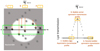 |
Fig. 1. Cartoon illustrating the Lyα transmission profile of galaxies in a plane of the sky around an ionized bubble. Left: Galaxies in and around a spherical bubble with the observer at the top. Right: The integrated Lyα transmissions, 𝒯 as a function of transverse distance (x) measured using galaxies in the green box in the left panel. Transmission profiles 𝒯(x) viewed in different windows (A, B, and C) are different. Window A: Galaxies are all outside the bubble and all have 𝒯 ≈ 0 , resulting in a flat transmission profile in the window. Window B: Galaxies are located around the center of the bubble, therefore 𝒯 in the window are all high and the transmission profile is symmetric around the window center. Window C: Half of the galaxies are outside the bubble and have 𝒯 ≈ 0 . The other half of the galaxies are inside the bubble, having rising transmission toward the bubble center. The transmission profile around the center of window C is therefore asymmetric. The level of asymmetry can therefore be a probe of bubble edges. |
If the transmission profile on the right and left of the window center are both low and flat (window A in the right panel of Figure 1), the window is outside a bubble. If the transmission profiles on both sides of a window are high and symmetric (window B in the right panel), the window is inside a bubble and close to the bubble center. If one side of a window has a flat and low transmission profile, and the other side has a rising transmission profile (window C in the right panel), the window is at the edge of a bubble. By defining and measuring an asymmetry score for these transmission profiles in windows at different positions in a field, it should be easy to detect bubble edges by identifying high asymmetry score regions.
We define an asymmetry vector for each position, r, in an observed field within a circular window using
 (5)
(5)
where Ngal, window is the number of galaxies in the window centered at r, 𝒯i is the Lyα transmission of i-th galaxy, and ri=(rgal, i−r)/Rwindow is the position of the i-th galaxy with respect to the window center, normalized by the window radius (Rwindow). In practice, we calculate the asymmetry vector along the horizontal and vertical transverse directions. Looking at the center position of window C in the right panel of Figure 1, we see how Equation (5) reflects asymmetry along the x-axis. At the edge of the bubble, only galaxies in the +x direction have high transmission 𝒯i, thus the asymmetry vector will be positive with large magnitude. Moving into the center of the bubble, galaxies have high transmission equally in the −x and +x directions, thus A(x)→0. We define the asymmetry score as the magnitude of the asymmetry vector (|A|).
Figure 2 shows an example ionization map (left panel) and the asymmetry score map (middle panel) generated using the Lyα transmission of galaxies in that field (assuming perfect recovery of transmission). In addition, we show the asymmetry vector map (right panel). The asymmetry score map shows that at bubble edges, we recover high asymmetry scores as required. Asymmetry scores in bubble centers and neutral regions are low because of the flat transmission profile. The directions of asymmetry vectors point toward bubble edges. In this paper, for simplicity, we only use the asymmetry score to recover bubble maps. We do not use the direction information of the asymmetry vector in this work, but it is important to note that it could be used to further refine bubble finding algorithms.
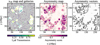 |
Fig. 2. Example of an asymmetry score map made using galaxies’ Lyα transmission. Left: Simulated ionization map (4 cMpc slice from our simulation with mean neutral fraction |

Figure 2 shows that high asymmetry score areas match real bubble edges. However, to define bubble edges we must calibrate a threshold in asymmetry. To do this, we convert both the input ionization map and asymmetry map into binary maps (neutral or ionized), and compare how similar the two maps are. Detailed descriptions of binary map conversion and calibration can be found in Appendix A.1. We find the best asymmetry score threshold, Athresh, to be Athresh = 0.3−0.4, and that it is independent of the IGM mean neutral fraction  , meaning it is possible to map bubbles using this method irrespective of the surrounding IGM conditions or bubble sizes.
In what follows, we calculate the asymmetry score using the peak value of the Lyα transmission posterior (i.e. the maximum likelihood value) estimated for each galaxy, described in Section 2.3.
3.2. Suggested parameter setup
Our method has three free parameters: asymmetry score threshold (Athresh), window radius (Rwindow), and window depth. Here we first discuss how altering each parameter changes the result, then recommend the choice of each parameter, finding a single set of parameters which describe bubbles well.
Asymmetry score threshold, Athresh, is used to convert asymmetry maps into binary bubble maps. Athresh affects the segmentation and the size of the recovered bubbles. A lower Athresh leads to bigger bubble sizes and smoother bubble shapes. When Athresh is set too high, the resulting bubbles no longer represent ionized regions, but the regions around the edges of bubbles.
Window radius, Rwindow, in our bubble finding algorithm determines the minimum recovered bubble size and the noise on bubble edge recovery, it should be roughly comparable to the minimum bubble radius. The asymmetry score map produced using a smaller Rwindow reflects the ionization fluctuations on a smaller scale, thus it can be good for finding small bubbles. On the other hand, a big bubble may be split into several small bubbles using a small Rwindow. Different reionization morphologies may require different optimal Rwindow. However, this mostly impacts the recovery of very small bubbles (≤10 cMpc). To decide on Rwindow, we also need to consider the number of galaxies available for calculating the asymmetry score in each window. A minimum Rwindow can be estimated using the surface density of galaxies Σgal. The window radius for a desired average number of galaxies per window, Nwindow, will be
 (6)
(6)
Window depth is the depth of the window in the redshift direction. It affects the minimum recovered bubble size and the number of galaxies in a field. A deeper window depth will include galaxies in a wider redshift range for the asymmetry map calculation, but will bury the signal from small bubbles.
In Appendix A we test the best Athresh, Rwindow, and window depth combination for  (i.e. before significant overlap of ionized regions, Miralda-Escudé et al. 2000). Encouragingly, we find the best Athresh (0.3), window radius (12 cMpc), and window depth (4 cMpc, Δz∼0.015 at z = 8) remain unchanged across the tested
  range, meaning our method works generically for a broad range of bubble sizes. We also test the minimum number of galaxies required to calculate the asymmetry score in a window, finding excluding windows with Nwindow<2 reduces noise in the recovered maps.
3.3. Observational requirements for mapping bubbles in the plane of the sky
We now consider what observational conditions are required to map ionized bubbles in the plane of the sky. We test the number density of sources sampled, and the maximum Lyα EW3 limit required to recover bubble edges. Full details of our tests are described in Appendix B and we summarize the key results here. We find we need to observe ≳0.004 galaxies/cMpc3 (corresponding to MUV≤−17.2 at z = 8) and a 5σ Lyα equivalent limit ≤30 Å for the faintest galaxies to obtain the best recovery of our simulated bubble maps: our algorithm can recover bubbles with R≳10 cMpc with <30% bubble size precision in this case, but that we can still trace bubbles well with slightly lower number density (≳0.002 galaxies/cMpc3, corresponding to MUV≤−17.8 at z = 8).
To fully map bubbles we need the field of view to be larger than bubble diameters. Typical bubble sizes depend on the reionization timeline and ionizing sources, which we discuss further in Section 5.1, but are expected to be R∼2−30 cMpc (R∼2−20 arcmin) during the first half of reionization (Lu et al. 2024). To accurately find bubble edges the field of view must also be larger than our window radius (12 cMpc ≈5 arcmin at z = 8). These areas are feasible with wide JWST surveys, particularly in the early stages of reionization.
Figure 3 shows the asymmetry maps made using Lyα transmission in our z = 8 simulations at  . We show the maps obtained using galaxies with ≈0.002 galaxies/cMpc3 (corresponding to MUV≤−17.8 at z = 8) and Lyα flux limit corresponding to a 5σ Lyα equivalent limit ≤30 Å for the faintest galaxies in the map (i.e. brighter galaxies have lower EW limits). We generate the maps by first using the Bayesian method in Section 2.3 to infer P(𝒯) for each galaxy given their observed EW, the uncertainty of EW, and MUV, then calculating asymmetry score at each sky position using the maximum likelihood of 𝒯 of galaxies around the position4. We set the asymmetry score to 0 for positions with fewer than 2 galaxies in the window to reduce noise in the recovered map.
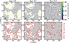 |
Fig. 3. Top panels: Ionization maps and galaxies colored by their Lyα transmissions, at |

In addition to the number density and flux limit requirements, we also require precise systemic redshift resolution. The window depth must be comparable to the diameter of typical bubbles – in the first half of reionization the median bubbles have radii of ≲10−30 cMpc (Lu et al. 2024). Thus, to capture these bubbles, asymmetry maps should be made using galaxies in a thin redshift window (window depth = 4 cMpc or Δz∼0.015 at z = 8, as described above in Section 3.2), requiring spectroscopic observations (i.e. narrow-bands are too broad to cover single bubbles during most of reionization, see also Sobacchi & Mesinger 2015, for similar conclusions).
Finally, to map entire ionized bubbles in the plane of the sky requires a field of view (FoV) that is larger than bubble diameters. For reference, the 1% largest ionized bubble diameter at  (0.9) is ∼300 (60) cMpc or ∼100 (20) arcmin for reionization driven by high mass halos (see Figure 10, also Lu et al. 2024). In the earliest stages of reionization (
 ), it should thus be feasible to map entire ionized regions with deep JWST observations.
Upcoming wide-area imaging and spectroscopy surveys, such as the Euclid Deep survey (Euclid Collaboration: Scaramella et al. 2022; van Mierlo et al. 2022; Marchetti et al. 2017), Roman High Latitude Spectroscopy Survey (HLSS; Wang et al. 2022), Subaru PFS (Greene et al. 2022), and VLT MOONS (Maiolino et al. 2020; Gagnon-Hartman et al. 2025; Mesinger et al. 2024), will observe thousands of reionization-era galaxies on >1 sq. deg scales required to cover multiple ionized regions in the mid-stages of reionization and observe their Lyα. However, these surveys will not be deep enough to recover bubble maps by themselves, using the method we describe here, as they will not reach the required galaxy number density and Lyα EW limits. However the bright Lyα emitters detected in these surveys should signpost large ionized regions and would provide ideal targets for deep spectroscopic follow-up with JWST. We will discuss observational prospects for mapping ionized regions in more detail in Section 5.1.
4. Mapping bubbles along the line-of-sight
JWST's field of view (spanning ≈10 cMpc at z∼8) can capture entire bubbles in the early stages of reionization, but JWST can also efficiently map ionized structures along the line-of-sight (LOS) direction at all stages of reionization. The median bubble size at the mid-point of reionization spans Δz∼0.1−0.3. JWST can detect galaxies over such a wide redshift window with precise systemic redshift resolution (R∼1000 corresponding to Δz≲0.001 with NIRSpec medium resolution grating and NIRCam grism spectroscopy, e.g. Tang et al. 2023; Oesch et al. 2023; Meyer et al. 2024). Here we describe a novel algorithm to recover bubble maps in redshift skewers using the LOS transmission profile.
Instead of the bell-shaped Lyα transmission profile for bubbles in the plane of the sky (Figure 1), the transmission profile in the LOS direction has a shark-fin-like shape (see Figure 4 for a cartoon illustration). As we move along the LOS away from the observer, the Lyα transmission changes as follows: in front of a bubble (closest to the observer), we expect almost no transmitted Lyα flux from galaxies. Stepping into the bubble, the closer a galaxy is to the back end of the bubble, the higher the Lyα transmission, because of the increasing path length of ionized IGM in front of galaxy. Galaxies at the back of the bubble have the highest Lyα transmission. When stepping out of the back size of the bubble, we again expect almost no transmitted Lyα flux from galaxies. Thus, the points of nonzero Lyα transmission should mark the edges of the bubble.
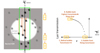 |
Fig. 4. Cartoon illustrating the transmission profile of galaxies along the LOS direction around a bubble. Left: Galaxies in and around a spherical bubble. Right: The integrated Lyα transmissions as a function of the LOS distance (d) measured using galaxies in the green box in the left panel. Transmission profiles (T)(z) viewed in different windows (A, B, and C) are different. Window A: Galaxies in front of the bubble are in fully neutral gas and thus experience a strong Lyα damping wing and have almost zero transmission. Stepping back into the bubble the transmission increases because of the increased path length of ionized IGM in front of galaxies. Window B: Galaxies located at the back of the bubble have the highest transmission because they have the longest path length through the ionized IGM. Window C: Galaxies on the far side of the bubble are in fully neutral IGM and have almost zero transmission. Galaxies’ integrated Lyα transmission is tightly correlated with the distance between the galaxy and the nearest neutral IGM patch along the LOS. We can use this correlation to map ionized regions along the LOS (Section 4). |
There is a tight correlation between a galaxy's integrated Lyα transmission 𝒯 and the line-of-sight distance from the galaxy to the first neutral patch, dIGM, which we can use to map the bubble. This is because the damping wing optical depth is dominated by the first neutral IGM along the line-of-sight (Mesinger & Furlanetto 2008). We derive 𝒯(dIGM) and its 16−84 percentile range numerically from our simulations by measuring the 𝒯 of galaxies with the same dIGM along 105 sightlines (Section 2.2). Figure 5 shows 𝒯(dIGM) in our simulation at z≈8 for  , 0.7, 0.9. We find 𝒯(dIGM) has negligible dependence on
  at fixed redshift. We also compare 𝒯(dIGM) for galaxies with emitted Lyα velocity offset ΔvLyα>200 km/s and ΔvLyα<200 km/s, finding 𝒯(dIGM) has only a small dependence on velocity offset once a galaxy is at least >10 cMpc from a neutral patch (see also, e.g. Endsley & Stark 2022; Prieto-Lyon et al. 2023). We see the variance (coming from the distribution of additional neutral patches along sightlines) of the 𝒯(dIGM) curve is also small, resulting in less than 10 cMpc under- or over-estimate of dIGM when estimating dIGM from 𝒯.
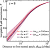 |
Fig. 5. Integrated Lyα transmission as a function of the distance between a galaxy and the first neutral IGM patch the galaxy light encounters at z = 8. Solid lines in orange, maroon, and black curves show 𝒯(dIGM) for all the galaxies at |


We note that the relation shown in Figure 5 is only valid for z = 8, as the damping wing optical depth increases with increasing redshift due to increasing gas density (Gunn & Peterson 1965), but the minimal dependence on  and velocity offset for >10 cMpc bubbles is qualitatively true at other redshifts.
Figure 6 shows a sightline in our simulation at  , selected in a sky area corresponding to 3 JWST NIRSpec footprints (42.8 arcmin2 at z = 8), collapsed along the y direction. We show ionized regions and the positions of all MUV<−17.5 galaxies. We also plot the integrated Lyα transmissions and Lyα EW of these galaxies as a function of LOS distance, along with our averaged 𝒯(dIGM) profile based on the positions and sizes of the recovered bubbles in the skewer. The Lyα transmissions of galaxies in each bubble follow our averaged profile very well, with all Lyα transmissions falling along or below the curve.
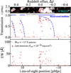 |
Fig. 6. Example sightline skewer showing galaxies’ Lyα transmissions and EW as a function of the LOS position, where the zero point of the LOS position is arbitrary. The top panel shows the ionization map in the x−z plane (white ionized, black neutral gas). Red empty and solid dots are galaxies with MUV>−17.5 in the slice. Red solid points are galaxies with fLyα>10−18 erg/s/cm2. The middle panel shows the Lyα transmission for each galaxy as a function of LOS position. Galaxies in bubbles show high transmission while galaxies in neutral IGM having transmission ≈0. Horizontal Gray lines show the spans of the simulated ionized bubbles along the sightline. Blue dashed lines are the 𝒯(dIGM) curves derived using the damping wing optical depth (Figure 5), galaxy transmissions follow this curve very well. The blue horizontal lines show the span of the recovered bubbles using our method (Section 4.1). The bottom panel shows the observed Lyα EW of the galaxies, highlighting that strong Lyα EW ≳ 50 Å likely signpost large ionized regions. |
The scatter of transmission below the 𝒯(dIGM) curve mainly comes from bubbles which are clumpy along the line of sight, so galaxies at the same redshift within the field of view are not necessarily at the same distance to neutral gas. A minor cause of the scatter of transmissions ( ) is the Lyα emission line velocity offset. A strongly red-shifted Lyα emission line (e.g. >300 km/s) will suffer less from the damping wing absorption and therefore have higher transmission than the expected value in our 𝒯(dIGM) relation.
In this paper we focus on estimating the maximum bubble diameter along the LOS. Therefore we want to find a 𝒯(dIGM) curve for each bubble which envelopes the observed transmission spikes, and thus marks the front and back of the bubble. In the next section we describe a simple algorithm to do this.
4.1. An algorithm for finding bubbles along the LOS
To detect bubbles along a LOS using Lyα transmission estimates, we develop a simple algorithm. For each galaxy we require an estimate of the integrated Lyα transmission (e.g. via comparing the observed Lyα EW to the predicted EW based on z∼5−6 observations, as described in Section 2.3), a precise systemic redshift (σ(z)<0.015) and sky coordinates so that we can make a 3D map of galaxy positions. The steps of the algorithm are as follows and illustrated in Figure 7:
-
Starting from the galaxy farthest away from the observer (galaxy with the highest redshift), gi, we invert the 𝒯(dIGM) curve (Figure 5) to estimate the distance from gi to the front of the bubble, Di using the estimated Lyα transmission of gi.
-
If gi is the first galaxy in a bubble, we set the redshift of the back of the bubble to the redshift of gi, zback=zi. We set the LOS bubble diameter Dbubble=Di, and mark all the galaxies within a distance Dbubble in front of gi to be in the same bubble as gi (panel a of Figure 7).
-
A galaxy's Lyα transmission may not follow exactly 𝒯(dIGM) due to an irregular bubble shape or over-predicted emergent Lyα line, and thus may fall below the 𝒯(dIGM) line. To make sure all the galaxies in the bubble have transmission falling on or below the 𝒯(dIGM) curve, we move to the next galaxy (galaxy with the second highest redshift), gi+1, a distance di, i+1 from gi. We estimate the distance of gi+1 from the neutral IGM, Di+1 by inverting 𝒯(dIGM) as above.
-
If Di+1+di, i+1>Dbubble, we update Dbubble→Di+n+di, i+n and again mark galaxies within the updated bubble (panel b of Figure 7).
-
By iterating through all the galaxies in the sightline, we can identify all the ionized bubbles (panel c of Figure 7).
To account for the uncertainty in Lyα transmission estimates we use the following approach. For each mock galaxy, we use the lower 16% bound on transmission inferred using the Bayesian approach described in Section 2.3 as the input 𝒯. We use this approach rather than the full inferred P(𝒯) or maximum likelihood 𝒯 because of the exponential-like relation between distance to HI and Lyα transmission (Figure 5), this would result in a bias to overestimated bubble sizes in our algorithm. We find using the lower bounds of 𝒯 always provides lower bound on bubble size that converges to the true bubble size when we include sufficient galaxies in the sightline (see Section 4.2).
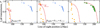 |
Fig. 7. Demonstration of our LOS-bubble-finding algorithm, where the zero point of the LOS position is arbitrary. (a) Starting from the galaxy farthest away from the observer, gi, we invert 𝒯(dIGM) (Figure 5, the red dashed line) to estimate the distance between the galaxy and the nearest neutral IGM patch, Di. We set the LOS bubble diameter, Dbubble=Di, and the redshift of the back of the bubble, zback=zi, that is, the redshift of the first galaxy. We then mark all galaxies in front of gi within Dbubble (orange dots) to be inside the same bubble as gi. (b) We then step through the bubble toward the observer to update our estimate of Dbubble. For a galaxy gi+n which is a distance di, i+n from galaxy gi we estimate the distance of galaxy gi+n from neutral IGM, Di+n. If Di+n+di, i+n>Dbubble we update Dbubble→Di+n+di, i+n. (c) Once we have iterated through all galaxies contained within Dbubble and Dbubble converges, we continue iterating through all the galaxies in the line-of-sight in the same manner to find all the bubbles. In this example sightline we find two bubbles and their associated galaxies (orange galaxies on the left and green galaxies on the right, the remaining blue point is a galaxy between the two bubbles and is not considered to be inside a bubble). |
4.2. Observational requirements for mapping bubbles along the line-of-sight
To detect bubbles along the line-of-sight requires (1) a good estimate of Lyα transmission for each galaxy, which depends on the Lyα EW limit, and (2) a sufficient number of galaxies in the line-of-sight to sample the region. To test the required observational constraints we apply our algorithm to sightlines extracted from our simulations, assuming different spectroscopic completeness and Lyα EW limits.
We sample 900 10 cMpc×10 cMpc×300 cMpc sightlines from our  simulation cube, corresponding to individual JWST NIRSpec pointings spanning Δz≈1 at z∼8. For each galaxy in each sightline, we infer P(𝒯) using the Bayesian approach in Section 2.3. We apply our algorithm to detect bubbles along these sightlines given galaxy positions and the lower limit of the inferred P(𝒯) (see discussion in Section 4.1 above).
In Figure 8 we plot the median recovered bubble diameter, Drecover, from our algorithm versus true bubble diameter, Dtrue, for ∼5000 bubbles. We calculate the true bubble positions and diameters in each sightline by collapsing the IGM skewer in both spatial directions, measuring the mean neutral fraction at each redshift position in the 1D skewer, and classify regions that have mean neutral fraction below xHI = 0.5 as ionized. We match the recovered bubbles to the true bubbles by iterating over the true bubbles and searching for recovered bubbles that overlap with them. If a true bubble has no corresponding recovered bubble, we record the size of the recovered bubble as 0 cMpc. If more than one recovered bubble overlaps with a true bubble, we count both recovered bubbles. We compare the results assuming a number density ≈0.004 galaxies/cMpc3 in each skewer (corresponding to complete spectroscopy of MUV≤−17.2 galaxies at z≈8 in our simulations) using Lyα flux limits corresponding to 5σ EW limits of 10−80 Å for the faintest galaxies (i.e. brighter galaxies will have lower EW limits). For >80 cMpc bubbles, the median recovered bubble size drops because some sightlines pass through big ionized bubbles but lack sufficient galaxies to sample the space, resulting in big ionized bubbles being recovered to be spatially close smaller bubbles. We note that this ‘bubble splitting’ issue can be reduced if the estimation of 𝒯 is improved.
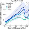 |
Fig. 8. Median recovered bubble size versus real bubble size for LOS bubbles assuming a number density of 0.004 galaxies/cMpc3 (corresponding to a complete spectroscopic sampling of galaxies down to MUV, limit=−17.2 at z≈8) for 5σ Lyα equivalent width limits = [10, 30, 50, 100] Å for the faintest galaxies (colored lines). The shaded region shows the 68% range of recovered bubble sizes for the Lyα equivalent width limit = 10 Å line. When the Lyα equivalent width limit is deeper than 50 Å we can estimate 𝒯 relatively well for each galaxy and thus we can recover bubble sizes ∼10−80 cMpc to within 30% of their true values (1−1 and 1−1±0.3 relations marked by solid gray lines). The dip at Rreal∼100 cMpc is due to sightlines that pass through a big bubble but without enough galaxies to sample the space, causing us to recover a few smaller bubbles instead of one big bubble. This could be improved in future work when 𝒯 can be more precisely estimated, for example, with a prior from the Lyα escape fraction (see Section 2.3). |
We see our algorithm can robustly recover the sizes of bubbles along sightlines extremely well, to ≲5% for Dtrue≈10−80 cMpc bubbles, providing the flux limit corresponds to a Lyα EW limit of ≲30 Å, roughly the median EW expected in a fully ionized IGM (see Section 2.3). Even with an EW limit of ≲50 Å we can obtain a lower limit on the bubble size within 30% of the true size. For true bubbles with Dtrue≲15 cMpc, we recover larger bubble diameters because we set the mean xHI threshold to 0.5 when identifying true bubbles in 1D skewers, which captures only the most ionized region at the center of small bubbles.
We find the number density of galaxies along a sightline is the dominant factor for the accuracy of the recovered bubble size. Figure 9 shows the ratio between recovered bubble size and real bubble size versus galaxy number density along sightlines, obtained by sampling recovered bubbles in our simulations varying the MUV, limit detection limit between −19 and −17 to sample a range of observed galaxy number densities. We find we can recover the true bubble size within <30% when the observed number density of galaxies reaches ≳0.004/cMpc3 and Drecover/Dtrue converges to ≈1 when ≳0.005/cMpc3. We recover a slightly larger (1.1−1.2×) median bubble size compared to the ‘true’ bubble size because of the irregular shapes of bubbles, where small ionized projections at the start or end of bubbles are identified via strong Lyα emission by our mapping algorithm but can be missed in our calculation of ‘true’ bubble positions in the 1D skewers. Future works carefully accounting for the 3D shapes of bubbles will improve the bubble size comparison.
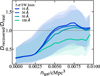 |
Fig. 9. Median recovered bubble size to real bubble size ratio (Drecovered/Dreal) versus galaxy number density for 5σ Lyα equivalent limits = [10, 30, 50, 100] Å (solid lines) binned by galaxy number density. Shaded regions show the 16−84 percentile of the recovered size ratio. The method converges to the correct bubble size as we reach ≳0.004 galaxies/cMpc3. |
We also test the effect of the systemic redshift uncertainty and find it has a minor impact on the recovered bubble size as long as it is smaller than the bubble diameter. We find our method requires a redshift uncertainty of σz≲0.015 (∼5 cMpc at z = 8). This requirement is achievable with JWST NIRSpec grating and NIRCam grism spectroscopy (which can measure Δz≈0.001).
5. Discussion
JWST's ability to spectroscopically confirm and detect Lyα from MUV≲−17 galaxies opens a new window on reionization, providing the potential to map ionized regions in four dimensions for the first time. This is a substantial step beyond the volume-averaged view we have had of the z>6 IGM prior to JWST (e.g., Stark et al. 2010; Schenker et al. 2014; Pentericci et al. 2014; Greig et al. 2017; Davies et al. 2018; Mason et al. 2018a; Jung et al. 2020; Bolan et al. 2022). We have developed ionized bubble mapping methods which, for the first time, use information from ensembles of galaxies (see also our companion paper, Nicolić et al., in prep.). In doing so, our methods mitigate the effects of intrinsic variability of Lyα transmission to enable robust estimates of the positions and sizes of ionized bubbles. In this section we discuss optimal strategies for mapping individual ionized regions to understand reionization on a local scale (Section 5.1) and prospects for constraining the bubble size distribution (Section 5.2).
5.1. Optimal observational strategies for mapping ionized regions
In Sections 3 and 4 we presented two simple methods for mapping ionized regions in the plane of the sky and along the line of sight. To map an ionized region and estimate its size requires observing a volume sufficient to detect the edges of the bubble, a sufficient number density of spectroscopically confirmed galaxies to trace the volume, ≳0.002−0.005 galaxies/cMpc3, systemic redshifts (i.e. from nonresonant lines such as [OIII]5007) with high redshift precision ≲0.015 to map galaxies on scales smaller than the expected bubble sizes, and deep Lyα observations, reaching 5σ rest-frame EW limits of ≈30 Å for the faintest (MUV∼−17) surveyed galaxies, to estimate the transmission of Lyα through the IGM, within reach of deep JWST observations (e.g., Jones et al. 2024; Tang et al. 2024a).
The required integration times to estimate Lyα transmission and determine the spectroscopic redshifts of galaxies are easily achievable for z∼7 galaxies and deep, but feasible, at z∼8. To achieve a 5-σ detection limit of 30 Å for Lyα emission from MUV∼−18.5 (−17.2) galaxies at z∼7 (z∼8) using the G140M filter on JWST, the integration time required is 2 hours (40 hours). For redshift confirmation using [O III] emission in MUV∼−18.5 (−17.2) galaxies at z∼7 (z∼8) with the G395M filter on JWST, the required integration time is 6 hours (130 hours), assuming that more than 90% of galaxies with MUV≲−18 have [O III] equivalent widths exceeding 120 Å (Endsley et al. 2024). For z∼8 sources, targeting galaxy overdensities would achieve the necessary galaxy number density with more reasonable integration times (e.g., Meyer et al. 2024; Tang et al. 2024a; Nikolić et al. 2025).
To understand the required volumes for mapping ionized bubbles in Figure 10 we show the diameter of ionized bubbles (median and 68% range) predicted by the simulations by Lu et al. (2024), in both the plane of the sky in arcmin (left axis) and along the line-of-sight in Δz (right axis) at z = 8. We show the predictions for two reionizing source models, a gradual reionization driven by galaxies in low mass (Mh>5×10⁸ M⊙) halos, versus a more rapid reionization driven by galaxies in higher mass halos (Mh>1011 M⊙). These models should span the expected range of bubble sizes. We compare the bubble sizes of ionized regions to the field of view of various JWST Cycle 1−3 spectroscopy surveys (assuming square survey areas): JADES GOODS-N + GOODS-S (Bunker et al. 2024), CEERS (Finkelstein et al. 2022) and COSMOS-3D (Kakiichi et al. 2024). We note only CEERS and JADES obtained Lyα spectra. As noted in Section 3.3, upcoming wide-area spectroscopic surveys with, for example, Roman, Euclid, PFS, MOONS (Cirasuolo et al. 2012; van Mierlo et al. 2022; Euclid Collaboration: Scaramella et al. 2022; Wang et al. 2022; Greene et al. 2022; Maiolino et al. 2020; Gagnon-Hartman et al. 2025; Mesinger et al. 2024) will span >1 sq. deg and contain many bubbles signposted by bright Lyα-emitters, but are not sensitive enough by themselves to detect the high number density of galaxies we need for mapping. Thus deep follow-up with JWST will be essential.
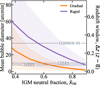 |
Fig. 10. Mean bubble diameter as a function of |

From Figure 10 it is clear that mapping whole ionized regions in the plane of the sky with JWST becomes most feasible when  . In the mid-stages of reionization (
 ) the field of view of the marked JWST surveys may be covered by a single ionized region. This is consistent with the high field-to-field variation in the Lyα fraction measured from current ∼100 sq. arcmin JWST fields (Napolitano et al. 2024; Tang et al. 2024a). Wide area JWST spectroscopy in fields with high Lyα detection fractions should be able to map whole bubbles in the mid-to-early stages of reionization. Figure 10 demonstrates that mapping bubbles along the line of sight is an efficient approach for estimating bubble sizes with JWST at all stages of reionization, as the largest bubbles at
  span Δz<0.7, which can be easily mapped with the wide wavelength coverage of JWST NIRSpec and NIRCam grism.
In the past few years, ground-based observations have found evidence for clustered Lyα emitters at z∼7 (e.g., Vanzella et al. 2011; Tilvi et al. 2020; Jung et al. 2022), implying the presence of ionized regions, but have been limited in the ability to detect Lyα from UV faint (MUV≳−20) galaxies. Excitingly, early JWST studies have demonstrated that comprehensively mapping bubbles along the line of sight is now finally feasible. Chen et al. (2024), Witstok et al. (2024) and Tang et al. (2024a) recently showed that with JWST spectroscopy it is possible to start mapping out the 3D distribution of galaxies and their Lyα around high EW (≳50 Å) Lyα-emitting galaxies, which likely signpost ionized regions. JWST has vastly increased the number of detectable sources compared to ground-based studies. Our line-of-sight bubble mapping method requires a density of ≳0.004 galaxies/cMpc3, corresponding to complete spectroscopic observations of MUV≳−18 (−17.2) galaxies at mean density at z≈7 (8) (e.g., Bouwens et al. 2021), but these densities could be obtained with a shallower detection limit in an overdense sightline, to obtain an estimate of the expected bubble size. The outlook for identifying and obtaining spectra of these required galaxy number densities is excellent with JWST: for example, around one of the strongest known z>7 Lyα emitters, JADES-13682 (z = 7.3, EW ≈ 400 Å, Saxena et al. 2023), estimates of a factor ∼7−25× overdensity have been reported using NIRCam imaging and grism spectroscopy (Endsley et al. 2023; Witstok et al. 2024; Tang et al. 2024a). Reaching EW ≈ 30 Å for MUV=−18 (−17.2) galaxies requires ≈8 (45) h with JWST NIRSpec (e.g., Jones et al. 2024; Tang et al. 2024a), feasible with deep JWST programs.
The methods we have presented here could be further refined in several ways in future work. As described in Section 2.3, estimates of Lyα escape fractions could be used as a prior on P(𝒯), which would further improve our estimates of the IGM transmission and thus bubble maps. Additionally, with deep high-resolution (R>2000) spectroscopy to resolve the Lyα lineshape at high S/N, it could be possible infer the wavelength-dependent damping wing attenuation (Mason & Gronke 2020), rather than just the integrated transmission. This would provide a more precise estimate of Lyα transmission for each galaxy and thus of the bubble size and position (Nikolić et al. 2025). Furthermore, in this work we have not considered the impact of self-shielding systems on <cMpc scales inside ionized regions, which would add additional Lyα opacity (e.g., Bolton & Haehnelt 2013; Mesinger et al. 2015; Mason & Gronke 2020; Nasir et al. 2021). However, these absorbers are predicted to be small (≈1−20 ckpc) and not uniformly distributed in the IGM and thus the probability of the majority of galaxies intersecting an absorber along the line of sight is low. We note that Chen et al. (2024) demonstrated that strong small-scale (<100 pkpc) galaxy overdensities may contain dense neutral gas which attenuates Lyα, though this is on much smaller scales than the expected sizes of bubbles. Future systematic observations of Lyα visibility as a function of overdensity will be important for understanding systematics in our methods due to residual neutral gas in ionized regions. However, as our methods utilize ensembles of galaxies and rely on ‘edges’ in Lyα transmission at fixed redshift, rather than absolute transmission, our approach should not be strongly impacted by the inclusion or redshift evolution of local small-scale absorbers in the ionized IGM or CGM.
The prospects for obtaining larger samples of ionized regions along multiple sightlines are promising. Upcoming wide-area imaging and spectroscopic surveys as described above, and on-going Lyα narrow-band surveys (e.g., Ouchi et al. 2018; Hu et al. 2019) will provide thousands of bright z≳7 galaxy candidates and Lyα-emitters (flux ≳1×10⁻¹⁷ erg s−1 cm−2). At z≳7 these bright galaxies and Lyα-emitters are likely to trace overdensities and sit in ionized regions. These regions would be ideal for spectroscopic follow-up with JWST to spectroscopically confirm faint sources (MUV≳−18) to map overdensities in 3D and obtain Lyα spectroscopy to infer the bubble sizes. A key prediction of reionization simulations is that reionization starts in overdensities (e.g., Iliev et al. 2008; Mesinger & Furlanetto 2007; Trac & Gnedin 2011; Ocvirk et al. 2016; Hutter et al. 2021), with galaxy properties playing a role in shaping the size distribution of ionized regions (e.g., McQuinn et al. 2007b; Seiler et al. 2019; Lu et al. 2024). Larger samples would enable the first systematic tests of bubble sizes as a function of overdensity and galaxy properties to enable an understanding of reionization on a local scale as we could directly compare bubble sizes to the estimated ionizing emission from the detected galaxies in the region. This could provide new insight in the ionizing photon escape fraction, star formation histories of the visible galaxies, and the contribution of galaxies below JWST's detection limits.
5.2. Prospects for estimating the size distribution of ionized regions
With a sufficiently large survey it should be possible to infer the bubble size distribution as a function of redshift. This distribution is sensitive to the halo mass scale of the dominant ionizing sources with reionization driven by higher mass halos producing rarer, larger bubbles at fixed  compared to low mass halos, (e.g., McQuinn et al. 2007b; Seiler et al. 2019; Lu et al. 2024) and thus offers important insights in the drives of reionization.
Since mapping bubbles along sightlines does not require wide continuous survey areas, we could efficiently build up a ‘bubble size distribution’ using multiple JWST fields (with spatially separated pointings to avoid having to model correlations). We note this will require appropriate definition of bubble sizes for comparison between models and observations as our line-of-sight method compresses 3D information effectively into 1D skewers where we trace the distribution of ionized ‘lengths’ in the IGM.
To explore how many fields are necessary to estimate the bubble size distribution we perform a Monte Carlo simulation using our IGM simulations. We take 10 cMpc×10 cMpc×300 cMpc (corresponding to single JWST NIRSpec pointings spanning Δz≈1 at z∼8) from our simulation cubes, as described in Section 4.2. We use simulations spanning ![Mathematical equation: $ {\bar {x}}=[0.4{-}0.9] $](/articles/aa/full_html/2025/05/aa52912-24/aa52912-24-eq33.gif) to capture a range of bubble size distributions. We use our sightline bubble mapping technique to estimate the sizes of the ionized regions in each skewer.
to capture a range of bubble size distributions. We use our sightline bubble mapping technique to estimate the sizes of the ionized regions in each skewer.
In Figure 11 we plot the recovered mean bubble diameter as a function of the number of sightlines used, for simulations with different bubble size distributions, obtained from sampling 150 realizations of our sightlines. We see that we can distinguish differences in mean bubble diameter of ≳10 cMpc with just 15−30 independent sightlines. The prospects for building up samples of this number of sightlines is very feasible, for example, JWST pure-parallel NIRCam imaging and slitless spectroscopy surveys are observing ≳200 pointings in Cycles 1−3 which would be ideal for spectroscopic follow-up (e.g., Williams et al. 2021; Morishita et al. 2023; Egami et al. 2024), and Lyα spectroscopy has already been obtained in four independent sightlines in Cycles 1−2 (Tang et al. 2023, 2024a; Jung et al. 2024; Jones et al. 2024; Napolitano et al. 2024).
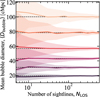 |
Fig. 11. Mean bubble diameter recovered from measuring bubbles along NLOS sightlines using our bubble mapping algorithm (Section 4), for simulations with different bubble-size distributions. The solid and shaded regions show the median and 68% range of the recovered mean bubble size from 150 realizations. With ≳15−30 sightlines it would be possible to distinguish different bubble size distributions. |
6. Conclusions
JWST provides our first opportunity to chart the reionization process in four dimensions. In this paper, we develop two simple methods to map ionized bubbles using ensembles of galaxies, allowing us to average over variation in intrinsic Lyα emission. Our main conclusions are as follows:
-
We develop an edge detection algorithm to map ionized bubbles in the plane of the sky, based on the asymmetry of Lyα transmission at each position on the sky. We test our method over an IGM neutral fraction range of xHI = 0.4−0.9. Our method is independent of
 and can robustly map bubbles ≳10 cMpc.
 -
Mapping bubbles in the plane of the sky requires a galaxy number density of ≳0.002 galaxies/cMpc3 (corresponding to MUV≲−18.5 (−17.8) at z∼7 (8), e.g. Bouwens et al. 2021) to trace the density field (with the most precise recovery for ngal≳0.004/cMpc3), survey areas greater than the typical sizes of ionized regions (∼25−3600 arcmin2 for
 ), and accurate galaxy redshift determination (Δz≲0.015). We require a 5σ Lyα equivalent width limit of ≲30 Å for the faintest galaxies. These sensitivity requirements are not within reach of currently planned wide-area spectroscopic surveys (PFS, MOONS, Euclid-Deep, Roman HLS), however these surveys will find bright Lyα-emitters which likely signpost large ionized regions and are thus ideal for deeper follow-up with JWST. Covering the areas required for mapping bubbles will be possible in the early stages of reionization with wide-area JWST spectroscopy.
 -
An efficient strategy to map bubbles at all stages of reionization with JWST is along the line-of-sight, which can be performed even in a single NIRSpec pointing, as bubble diameters are expected to span a redshift range Δz∼0.05−0.6 for
 . We develop an algorithm which makes use of the nearly one-to-one relation between integrated Lyα transmission and distance from a galaxy to the first neutral IGM patch, the relation is calibrated using inhomogeneous large-scale IGM simulations (Lu et al. 2024).
 -
The spectroscopic and imaging capabilities of JWST already provide the sensitivity to map bubbles along the line-of-sight. We find we require a number density of ≳0.004 galaxies/cMpc3 and EW limit of ≈30 Å to accurately recover bubbles ≳10 cMpc along the line-of-sight, which is attainable with deep spectroscopy of MUV≲−18 (−17.2) sources at z≈7 (8), and/or in overdensities of brighter sources. For individual galaxy detections, we require integration times of ∼2 (40) hours to detect Lyα and ∼6 (130) hours to detect [OIII] for MUV∼−18.5 (−17.2) galaxies at z∼7 (8). Given these requirements, mapping bubbles at z≈7 is feasible with current spectroscopic efforts, while for z≈8, targeting overdensity fields is necessary to reduce integration time constraints and improve survey completeness. Shallower observations should still provide robust lower limits on bubble sizes.
Early JWST studies have already demonstrated the potential of JWST spectroscopy to map the 3D distribution of galaxies in ionized regions (Chen et al. 2024; Witstok et al. 2024; Tang et al. 2024a). By constraining the sizes of these ionized regions based on estimates of galaxies’ Lyα transmission we will be able to link galaxies directly to the growth of ionized regions, enabling a local understanding of reionization. Additional constraints on IGM transmission from Lyα escape fractions and line profiles will further improve bubble mapping methods, potentially reducing constraints on galaxy number densities (Nikolić et al. 2025). Accurate bubble maps will provide the opportunity for ionized photon ‘accounting’: enabling constraints on the escape fraction at z>6 and the ionizing contribution of galaxies below JWST's detection limits. Future observations, sampling a range of environments, could start to estimate the size distribution of ionized regions and quantitatively establish how overdensity is linked to the growth of ionized regions.
Data availability
Our code to create ionized bubble maps in the plane of the sky and along sightlines given galaxy positions, MUV, Lyα flux, and redshifts is publicly available here: https://github.com/ting-yi-lu/bubble_mapping_paper
Acknowledgments
The authors thank the anonymous referee for insightful comments. We thank Dan Stark for useful discussions. TYL, CAM and AH acknowledge support by the VILLUM FONDEN under grant 37459. CAM acknowledges support from the Carlsberg Foundation under grant CF22-1322. AM acknowledges support from the Italian Ministry of Universities and Research (MUR) through the PRIN project “Optimal inference from radio images of the epoch of reionization”, the PNRR project “Centro Nazionale di Ricerca in High Performance Computing, Big Data e Quantum Computing”. The Cosmic Dawn Center (DAWN) is funded by the Danish National Research Foundation under grant DNRF140. This work has been performed using the Danish National Life Science Supercomputing Center, Computerome.
Beyond this distance, HI contributes negligibly to damping wing absorption (Mesinger & Furlanetto 2008).
We use Lyα EW limit instead of flux sensitivity because in our case the technique is most sensitive to the EW limit, as we need to detect deviations from the EW distribution for the ionized IGM (Section 2.3).
We use the maximum likelihood of 𝒯 rather than sampling from the inferred P(𝒯) distributions because when the EW limit is shallow, P(𝒯) is very broad, which we found leads to many false bubbles in the recovered maps. Using the maximum likelihood 𝒯 means that galaxies where the transmission is well constrained to 𝒯 ≈ 0 or 𝒯 ≈ 1 contribute most to the asymmetry score, improving the recovery of the bubbles. This is further demonstrated in Appendix B.2.
References
- Bhagwat, A., Napolitano, L., Pentericci, L., Ciardi, B., & Costa, T. 2024, ArXiv e-prints [arXiv:2408.16063] [Google Scholar]
- Blaizot, J., Garel, T., Verhamme, A., et al. 2023, MNRAS, 523, 3749 [NASA ADS] [CrossRef] [Google Scholar]
- Bolan, P., Lemaux, B. C., Mason, C., et al. 2022, MNRAS, 517, 3263 [Google Scholar]
- Bolan, P., Bradăc, M., Lemaux, B. C., et al. 2024, MNRAS, 531, 2998 [Google Scholar]
- Bolton, J. S., & Haehnelt, M. G. 2013, MNRAS, 429, 1695 [Google Scholar]
- Bosman, S. E. I., Davies, F. B., Becker, G. D., et al. 2022, MNRAS, 514, 55 [NASA ADS] [CrossRef] [Google Scholar]
- Bouwens, R. J., Oesch, P. A., Stefanon, M., et al. 2021, AJ, 162, 47 [NASA ADS] [CrossRef] [Google Scholar]
- Bowman, J. D., Cairns, I., Kaplan, D. L., et al. 2013, PASA, 30, e031 [Google Scholar]
- Bunker, A. J., Cameron, A. J., Curtis-Lake, E., et al. 2024, A&A, 690, A288 [NASA ADS] [CrossRef] [EDP Sciences] [Google Scholar]
- Carniani, S., Hainline, K., D’Eugenio, F., et al. 2024, Nature, 633, 318 [CrossRef] [Google Scholar]
- Castellano, M., Dayal, P., Pentericci, L., et al. 2016, ApJ, 818, L3 [NASA ADS] [CrossRef] [Google Scholar]
- Chen, Z., Stark, D. P., Mason, C., et al. 2024, MNRAS, 528, 7052 [CrossRef] [Google Scholar]
- Cirasuolo, M., Afonso, J., Bender, R., et al. 2012, SPIE Conf. Ser., 8446, 84460S [Google Scholar]
- Curtis-Lake, E., Carniani, S., Cameron, A., et al. 2023, Nat. Astron., 7, 622 [NASA ADS] [CrossRef] [Google Scholar]
- Davies, F. B., Hennawi, J. F., Bañados, E., et al. 2018, ApJ, 864, 142 [NASA ADS] [CrossRef] [Google Scholar]
- Dijkstra, M., Mesinger, A., & Wyithe, J. S. B. 2011, MNRAS, 414, 2139 [NASA ADS] [CrossRef] [Google Scholar]
- Egami, E., Fan, X., Sun, F., et al. 2024, SAPPHIRES: Slitless Areal Pure-Parallel High-Redshift Emission Survey, JWST Proposal. Cycle 3, 6434 [Google Scholar]
- Eilers, A. -C., Mackenzie, R., Pizzati, E., et al. 2024, ApJ, 974, 275 [NASA ADS] [CrossRef] [Google Scholar]
- Endsley, R., & Stark, D. P. 2022, MNRAS, 511, 6042 [NASA ADS] [CrossRef] [Google Scholar]
- Endsley, R., Stark, D. P., Whitler, L., et al. 2023, MNRAS, 524, 2312 [NASA ADS] [CrossRef] [Google Scholar]
- Endsley, R., Stark, D. P., Whitler, L., et al. 2024, MNRAS, 533, 1111 [NASA ADS] [CrossRef] [Google Scholar]
- Euclid Collaboration (Scaramella, R., et al.) 2022, A&A, 662, A112 [NASA ADS] [CrossRef] [EDP Sciences] [Google Scholar]
- Fan, X., Strauss, M. A., Becker, R. H., et al. 2006, AJ, 132, 117 [NASA ADS] [CrossRef] [Google Scholar]
- Finkelstein, S. L., Bagley, M. B., Arrabal Haro, P., et al. 2022, ApJ, 940, L55 [NASA ADS] [CrossRef] [Google Scholar]
- Gagnon-Hartman, S., Davies, J., & Mesinger, A. 2025, A&A, submitted [arXiv:2502.20447] [NASA ADS] [CrossRef] [EDP Sciences] [Google Scholar]
- Garel, T., Blaizot, J., Rosdahl, J., et al. 2021, MNRAS, 504, 1902 [NASA ADS] [CrossRef] [Google Scholar]
- Greene, J., Bezanson, R., Ouchi, M., Silverman, J., & the PFS Galaxy Evolution Working Group 2022, ArXiv e-prints [arXiv:2206.14908] [Google Scholar]
- Greig, B., Mesinger, A., Haiman, Z., & Simcoe, R. A. 2017, MNRAS, 466, 4239 [Google Scholar]
- Gunn, J. E., & Peterson, B. A. 1965, ApJ, 142, 1633 [Google Scholar]
- Haiman, Z. 2002, ApJ, 576, L1 [NASA ADS] [CrossRef] [Google Scholar]
- Hayes, M. J., & Scarlata, C. 2023, ApJ, 954, L14 [NASA ADS] [CrossRef] [Google Scholar]
- Hayes, M. J., Runnholm, A., Scarlata, C., Gronke, M., & Rivera-Thorsen, T. E. 2023, MNRAS, 520, 5903 [NASA ADS] [CrossRef] [Google Scholar]
- Heintz, K. E., Brammer, G. B., Watson, D., et al. 2025, A&A, 693, A60 [Google Scholar]
- Helton, J. M., Sun, F., Woodrum, C., et al. 2024, ApJ, 962, 124 [NASA ADS] [CrossRef] [Google Scholar]
- Hu, W., Wang, J., Zheng, Z. -Y., et al. 2019, ApJ, 886, 90 [NASA ADS] [CrossRef] [Google Scholar]
- Hutter, A., Trott, C. M., & Dayal, P. 2018, MNRAS, 479, L129 [Google Scholar]
- Hutter, A., Dayal, P., Yepes, G., et al. 2021, MNRAS, 503, 3698 [NASA ADS] [CrossRef] [Google Scholar]
- Hutter, A., Heneka, C., Dayal, P., et al. 2023, MNRAS, 525, 1664 [Google Scholar]
- Iliev, I. T., Shapiro, P. R., McDonald, P., Mellema, G., & Pen, U. -L. 2008, MNRAS, 391, 63 [Google Scholar]
- Jaccard, P. 1912, New Phytologist, 11, 37 [Google Scholar]
- Jakobsen, P., Ferruit, P., Alves de Oliveira, C., et al. 2022, A&A, 661, A80 [NASA ADS] [CrossRef] [EDP Sciences] [Google Scholar]
- Jaskot, A. E., Dowd, T., Oey, M. S., Scarlata, C., & McKinney, J. 2019, ApJ, 885, 96 [Google Scholar]
- Jones, G. C., Bunker, A. J., Saxena, A., et al. 2024, A&A, 683, A238 [NASA ADS] [CrossRef] [EDP Sciences] [Google Scholar]
- Jones, G. C., Bunker, A. J., Saxena, A., et al. 2025, MNRAS, 536, 2355 [Google Scholar]
- Jung, I., Finkelstein, S. L., Dickinson, M., et al. 2020, ApJ, 904, 144 [NASA ADS] [CrossRef] [Google Scholar]
- Jung, I., Finkelstein, S. L., Larson, R. L., et al. 2022, ApJ, submitted [arXiv:2212.09850] [Google Scholar]
- Jung, I., Finkelstein, S. L., Arrabal Haro, P., et al. 2024, ApJ, 967, 73 [NASA ADS] [CrossRef] [Google Scholar]
- Kakiichi, K., Hennawi, J. F., Ono, Y., et al. 2023, MNRAS, 523, 1772 [Google Scholar]
- Kakiichi, K., Egami, E., Fan, X., et al. 2024, COSMOS-3D: A Legacy Spectroscopic/Imaging Survey of the Early Universe, JWST Proposal. Cycle 3, 5893 [Google Scholar]
- Larson, R. L., Finkelstein, S. L., Hutchison, T. A., et al. 2022, ApJ, 930, 104 [NASA ADS] [CrossRef] [Google Scholar]
- Lin, X., Cai, Z., Wu, Y., et al. 2024, ApJS, 272, 33 [NASA ADS] [CrossRef] [Google Scholar]
- Lu, T. -Y., Mason, C. A., Hutter, A., et al. 2024, MNRAS, 528, 4872 [CrossRef] [Google Scholar]
- Maiolino, R., Cirasuolo, M., Afonso, J., et al. 2020, The Messenger, 180, 24 [NASA ADS] [Google Scholar]
- Marchetti, L., Serjeant, S., & Vaccari, M. 2017, MNRAS, 470, 5007 [Google Scholar]
- Mason, C. A., & Gronke, M. 2020, MNRAS, 499, 1395 [Google Scholar]
- Mason, C. A., Trenti, M., & Treu, T. 2015, ApJ, 813, 21 [NASA ADS] [CrossRef] [Google Scholar]
- Mason, C. A., Treu, T., Dijkstra, M., et al. 2018a, ApJ, 856, 2 [Google Scholar]
- Mason, C. A., Treu, T., de Barros, S., et al. 2018b, ApJ, 857, L11 [Google Scholar]
- Mason, C. A., Trenti, M., & Treu, T. 2023, MNRAS, 521, 497 [NASA ADS] [CrossRef] [Google Scholar]
- McQuinn, M., Hernquist, L., Zaldarriaga, M., & Dutta, S. 2007a, MNRAS, 381, 75 [NASA ADS] [CrossRef] [Google Scholar]
- McQuinn, M., Lidz, A., Zahn, O., et al. 2007b, MNRAS, 377, 1043 [Google Scholar]
- Mesinger, A., & Furlanetto, S. 2007, ApJ, 669, 663 [Google Scholar]
- Mesinger, A., & Furlanetto, S. R. 2008, MNRAS, 385, 1348 [NASA ADS] [CrossRef] [Google Scholar]
- Mesinger, A., Furlanetto, S., & Cen, R. 2011, MNRAS, 411, 955 [Google Scholar]
- Mesinger, A., Aykutalp, A., Vanzella, E., et al. 2015, MNRAS, 446, 566 [Google Scholar]
- Mesinger, A., Greig, B., & Sobacchi, E. 2016, MNRAS, 459, 2342 [NASA ADS] [CrossRef] [Google Scholar]
- Mesinger, A., Ciardi, B., Davies, J. E., Gagnon-Hartman, S., & D’Odorico, V. 2024, The Messenger, 193, 24 [Google Scholar]
- Meyer, R. A., Oesch, P. A., Giovinazzo, E., et al. 2024, MNRAS, 535, 1067 [CrossRef] [Google Scholar]
- Miralda-Escude, J. 1998, ApJ, 501, 15 [CrossRef] [Google Scholar]
- Miralda-Escude, J., & Rees, M. J. 1998, ApJ, 497, 21 [Google Scholar]
- Miralda-Escudé, J., Haehnelt, M., & Rees, M. J. 2000, ApJ, 530, 1 [CrossRef] [Google Scholar]
- Morishita, T., Mason, C., Trenti, M., et al. 2023, A NIRCam Pure-Parallel Imaging Survey of Galaxies Across the Universe, JWST Proposal. Cycle 2, 3990 [Google Scholar]
- Nakane, M., Ouchi, M., Nakajima, K., et al. 2024, ApJ, 967, 28 [NASA ADS] [CrossRef] [Google Scholar]
- Napolitano, L., Pentericci, L., Santini, P., et al. 2024, A&A, 688, A106 [NASA ADS] [CrossRef] [EDP Sciences] [Google Scholar]
- Nasir, F., Cain, C., D’Aloisio, A., Gangolli, N., & McQuinn, M. 2021, ApJ, 923, 161 [Google Scholar]
- Neufeld, D. A. 1991, ApJ, 370, L85 [Google Scholar]
- Nikolić, I., Mesinger, A., Mason, C. A., et al. 2025, A&A, submitted [arXiv:2501.07980] [Google Scholar]
- Ning, Y., Cai, Z., Lin, X., et al. 2024, ApJ, 963, L38 [NASA ADS] [CrossRef] [Google Scholar]
- Ocvirk, P., Gillet, N., Shapiro, P. R., et al. 2016, MNRAS, 463, 1462 [Google Scholar]
- Oesch, P. A., Dokkum, P. G. V., Illingworth, G. D., et al. 2015, ApJ, 804, L30 [CrossRef] [Google Scholar]
- Oesch, P. A., Brammer, G., Naidu, R. P., et al. 2023, MNRAS, 525, 2864 [NASA ADS] [CrossRef] [Google Scholar]
- Ouchi, M., Harikane, Y., Shibuya, T., et al. 2018, PASJ, 70, S13 [Google Scholar]
- Oyarzún, G. A., Blanc, G. A., González, V., Mateo, M., & Bailey, J. I. 2017, ApJ, 843, 133 [CrossRef] [Google Scholar]
- Park, H., Jung, I., Song, H., et al. 2021, ApJ, 922, 263 [NASA ADS] [CrossRef] [Google Scholar]
- Pentericci, L., Vanzella, E., Fontana, A., et al. 2014, ApJ, 793, 113 [NASA ADS] [CrossRef] [Google Scholar]
- Prieto-Lyon, G., Mason, C., Mascia, S., et al. 2023, ApJ, 956, 136 [NASA ADS] [CrossRef] [Google Scholar]
- Qin, Y., Mesinger, A., Bosman, S. E. I., & Viel, M. 2021, MNRAS, 506, 2390 [NASA ADS] [CrossRef] [Google Scholar]
- Reddy, N. A., Steidel, C. C., Pettini, M., Bogosavljević, M., & Shapley, A. E. 2016, ApJ, 828, 108 [Google Scholar]
- Ren, K., Trenti, M., & Mutch, S. J. 2018, ApJ, 856, 81 [Google Scholar]
- Roberts-Borsani, G. W., Bouwens, R. J., Oesch, P. A., et al. 2016, ApJ, 823, 143 [NASA ADS] [CrossRef] [Google Scholar]
- Santos, M. R. 2004, MNRAS, 349, 1137 [NASA ADS] [CrossRef] [Google Scholar]
- Saxena, A., Robertson, B. E., Bunker, A. J., et al. 2023, A&A, 678, A68 [NASA ADS] [CrossRef] [EDP Sciences] [Google Scholar]
- Saxena, A., Bunker, A. J., Jones, G. C., et al. 2024, A&A, 684, A84 [NASA ADS] [CrossRef] [EDP Sciences] [Google Scholar]
- Schenker, M. A., Ellis, R. S., Konidaris, N. P., & Stark, D. P. 2014, ApJ, 795, 20 [NASA ADS] [CrossRef] [Google Scholar]
- Seiler, J., Hutter, A., Sinha, M., & Croton, D. 2019, MNRAS, 487, 5739 [CrossRef] [Google Scholar]
- Shapiro, P. R., & Giroux, M. L. 1987, ApJ, 321, L107 [NASA ADS] [CrossRef] [Google Scholar]
- Shapley, A. E., Steidel, C. C., Pettini, M., & Adelberger, K. L. 2003, ApJ, 588, 65 [Google Scholar]
- Shen, Y., Strauss, M. A., Oguri, M., et al. 2007, AJ, 133, 2222 [NASA ADS] [CrossRef] [Google Scholar]
- Sheth, R. K., Mo, H. J., & Tormen, G. 2001, MNRAS, 323, 1 [NASA ADS] [CrossRef] [Google Scholar]
- Smith, A., Bromm, V., & Loeb, A. 2017, MNRAS, 464, 2963 [NASA ADS] [CrossRef] [Google Scholar]
- Sobacchi, E., & Mesinger, A. 2014, MNRAS, 440, 1662 [NASA ADS] [CrossRef] [Google Scholar]
- Sobacchi, E., & Mesinger, A. 2015, MNRAS, 453, 1843 [Google Scholar]
- Stark, D. P., Ellis, R. S., Chiu, K., Ouchi, M., & Bunker, A. 2010, MNRAS, 408, 1628 [Google Scholar]
- Stark, D. P., Ellis, R. S., & Ouchi, M. 2011, ApJ, 728, L2 [Google Scholar]
- Stark, D. P., Ellis, R. S., Charlot, S., et al. 2017, MNRAS, 464, 469 [NASA ADS] [CrossRef] [Google Scholar]
- Tang, M., Stark, D. P., Chen, Z., et al. 2023, MNRAS, 526, 1657 [NASA ADS] [CrossRef] [Google Scholar]
- Tang, M., Stark, D. P., Topping, M. W., Mason, C., & Ellis, R. S. 2024a, ApJ, 975, 208 [NASA ADS] [CrossRef] [Google Scholar]
- Tang, M., Stark, D. P., Ellis, R. S., et al. 2024b, MNRAS, 531, 2701 [NASA ADS] [CrossRef] [Google Scholar]
- Tilvi, V., Malhotra, S., Rhoads, J. E., et al. 2020, ApJ, 891, L10 [NASA ADS] [CrossRef] [Google Scholar]
- Topping, M. W., Stark, D. P., Endsley, R., et al. 2024, MNRAS, 529, 4087 [NASA ADS] [CrossRef] [Google Scholar]
- Torralba-Torregrosa, A., Matthee, J., Naidu, R. P., et al. 2024, A&A, 689, A44 [NASA ADS] [CrossRef] [EDP Sciences] [Google Scholar]
- Trac, H. Y., & Gnedin, N. Y. 2011, Adv. Sci. Lett., 4, 228 [Google Scholar]
- Treu, T., Trenti, M., Stiavelli, M., Auger, M. W., & Bradley, L. D. 2012, ApJ, 747, 27 [NASA ADS] [CrossRef] [Google Scholar]
- Umeda, H., Ouchi, M., Nakajima, K., et al. 2024, ApJ, 971, 124 [NASA ADS] [CrossRef] [Google Scholar]
- van Mierlo, S. E., Caputi, K. I., Ashby, M., et al. 2022, A&A, 666, A200 [NASA ADS] [CrossRef] [EDP Sciences] [Google Scholar]
- Vanzella, E., Pentericci, L., Fontana, A., et al. 2011, ApJ, 730, L35 [NASA ADS] [CrossRef] [Google Scholar]
- Verhamme, A., Orlitová, I., Schaerer, D., & Hayes, M. 2015, A&A, 578, A7 [NASA ADS] [CrossRef] [EDP Sciences] [Google Scholar]
- Wang, Y., Zhai, Z., Alavi, A., et al. 2022, ApJ, 928, 1 [Google Scholar]
- Whitler, L. R., Mason, C. A., Ren, K., et al. 2020, MNRAS, 495, 3602 [Google Scholar]
- Whitler, L., Stark, D. P., Endsley, R., et al. 2024, MNRAS, 529, 855 [CrossRef] [Google Scholar]
- Williams, C. C., Oesch, P., Barrufet, L., et al. 2021, PANORAMIC – A Pure Parallel Wide Area Legacy Imaging Survey at 1–5 Micron, JWST Proposal. Cycle 1, 2514 [Google Scholar]
- Witstok, J., Smit, R., Saxena, A., et al. 2024, A&A, 682, A40 [NASA ADS] [CrossRef] [EDP Sciences] [Google Scholar]
- Wold, I. G. B., Malhotra, S., Rhoads, J., et al. 2022, ApJ, 927, 36 [NASA ADS] [CrossRef] [Google Scholar]
- Yang, H., Malhotra, S., Rhoads, J. E., & Wang, J. 2017, ApJ, 847, 38 [NASA ADS] [CrossRef] [Google Scholar]
- Yatawatta, S., de Bruyn, A. G., Brentjens, M. A., et al. 2013, A&A, 550, A136 [NASA ADS] [CrossRef] [EDP Sciences] [Google Scholar]
- Zackrisson, E., Majumdar, S., Mondal, R., et al. 2020, MNRAS, 493, 855 [Google Scholar]
Appendix A: Optimizing bubble map recovery from asymmetry maps
Here we describe how we calibrate the parameters used for our asymmetry mapping technique (Section 3). We describe how we compare the recovered maps to the simulated ionization maps in Appendix A.1, our comparison metric in Appendix A.2 and the shape of the window function for creating asymmetry maps in Appendix A.3.
A.1. Creating binary  and asymmetry maps
The asymmetry map corresponds to the positions of bubble edges, not the positions of ionized regions. To compare the recovered asymmetry maps to the original ionization maps, we need to fill the recovered bubble edges. Here we describe how we convert the asymmetry and the original ionization maps into binary maps, in which 0 (1) in the map means neutral (ionized).
We convert our simulated ionization maps into binary maps to compare with our recovered maps. We first collapse the 3D ionization cubes into 2D binary maps by taking the mean neutral fraction over the line-of-sight direction. We then convert the neutral fraction at each sky position into a binary value by setting the position to be ionized if its mean neutral fraction is less than 0.5. The lower panel in Figure A.1 shows the mean neutral fraction for the ionization slice (first column) and the binary ionization map.
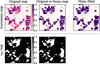 |
Fig. A.1. Example of converting an asymmetry score map into a binary ionization map (top panel), and converting an ionization map into a binary ionization map (bottom panel). The left column shows the original maps. The second column shows the maps converted into binary maps by setting all the pixels with asymmetry score ( |

To convert the asymmetry maps to binary maps we first set an asymmetry score threshold (Athresh). Pixels with asymmetry score above (below) the threshold are marked as ionized (neutral). We find Athresh≈0.3−0.4 provides the best map recovery (see below). In the upper panel of Figure A.1, we show an original asymmetry map in the first column and the binary map in the second column.
Secondly, since high asymmetry scores reflect bubble edges, we use the scipy.ndimage function, binary_fill_holes, to fill the closed outlines in the binary asymmetry map. The final binary asymmetry map is shown in the upper right corner in Figure A.1.
Figure A.2 shows the asymmetry maps made using different Athresh for a window radius of 12 cMpc and depth of 4 cMpc (see Section 3.1 for a description of the window). As Athresh increases, the recovered bubbles become more fractured. This is because the asymmetry scores around bubble edges are not constant. Only a few areas around bubble edges have very high asymmetry scores. If we only connect these high asymmetry score points, the recovered bubble becomes small and fractured. We find Athresh>0.5 will result in too many small bubbles.
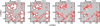 |
Fig. A.2. Recovered bubble maps using different Athresh. From left to right column are the maps using Athresh of 0.2,0.4,0.6,0.8, respectively. When Athresh>0.5, the recovered bubbles break into too many small pieces. |
We test for the best Athresh using our z = 8 simulations, assuming we can detect all the galaxies with MUV≤−17.8 (corresponding to 0.002 galaxies/cMpc3) and a 5σ Lyα EW detection limit of 30 Å (an optimistic observational requirement, see Appendix B.1). We vary Athresh between 0.15 and 0.4 and use a combination of visual and the Jaccard index (see Appendix A.2) to find the best Athresh≈0.3. We find this Athresh≈0.3 is independent of the IGM neutral fraction for  , and does not depend strongly on the window size (Appendix A.3), making it a robust, model-independent, choice for making bubble maps.
A.2. Comparison metrics
To evaluate the recovery of the bubble maps relative to the input ionization map we use the Jaccard index (𝒥, Jaccard 1912). This is defined as the fraction of correctly recovered ionized and neutral pixels in the following map:
 (A.1)
(A.1)
The Jaccard index directly reflects how good our recovered map is compared to the input one. 𝒥 = 0 (𝒥 > 0.8) means the recovered map is completely different from (the same as) the input map. By visual inspection of a range of maps at different  from our simulations, we found
  indicates a good recovery of bubble maps.
In Figure A.3 we show the values of Jaccard index for different window radius and depth combinations at  = 0.4-0.9. The Jaccard index clearly traces the optimum parameters until
  , when the mean bubble size becomes small and most of the field is neutral. Thus we use a combination of the Jaccard index with visual inspections of the maps to establish the best parameters for our method.
 |
Fig. A.3. Jaccard index for different window radius and depth combinations as a function of |

A.3. Optimal window shape
To determine the best window radius and depth combination for the asymmetry score (Equation 5), we calculate the Jaccard index for test window radii and depths for simulations at  = 0.4-0.9 (Figure A.3). We fix the Athresh = 0.4. We find the best recovery is for window radius <30 cMpc and window depth<25cMpc. For window depth <30cMpc the best window radius and depth are anticorrelated. This is because as the window depth increases, the true bubbles in the stacked ionization map become smaller, a small window radius is optimal to resolve small true bubbles. The window depth needs to be thin enough to prevent ionized bubbles from being washed out in the stacked ionization maps, but thick enough to include sufficient to sample the space. By visual inspection, we find the best parameters for our entire test
  range are [window radius, window depth]=[12, 4]cMpc.
Appendix B: Tests of observational requirements for asymmetry maps
Here we describe the number density of sources and Lyα EW limit required to map bubbles in the plane of the sky.
B.1. Required galaxy number density
To test the required number density of sources for creating robust asymmetry maps, we create a series of mock surveys at z = 8 varying the UV magnitude limit, MUV, limit, of detectable sources, assuming a 5σ Lyα EW detection limit of 30 Å for the faintest sources. We infer Lyα transmissions of individual galaxies using the Bayesian method as described in Section 2.2, using the maximum likelihood value of 𝒯. We use a combination of visual inspection and the Jaccard index to judge how well the input bubble maps are recovered.
Figure B.1 shows the recovered bubble maps for ngal≈0.0040, 0.0025, 0.0015, 0.0009, and 0.0005/cMpc3 at  . We find excellent recovery of bubbles for ngal≥0.002/cMpc3. Lower galaxy number densities do not sufficiently sample the space, resulting in recovered bubbles only centered around the strongest galaxy overdensities.
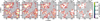 |
Fig. B.1. Recovered bubble maps corresponding to different galaxy number densities ngal≈0.0040−0.0005/cMpc3 at |

B.2. Required EW limit
To estimate the EW limit requirements for mapping bubbles using the asymmetry method, we create mock surveys at a range of  now varying the Lyα EW limit, EWLyα, limit for the faintest observable galaxies (i.e. we vary the flux limit, so brighter galaxies will have lower EW limits), assuming ngal = 0.004/cMpc3 (MUV, limit=−17.2 at z = 8). Figure B.2 shows example asymmetry maps at
  using EWLyα, limit = 10−100 Å for the faintest galaxies.
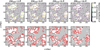 |
Fig. B.2. Upper panel: Input ionization map (gray neutral, white ionized) at |

As expected, we can recover bubble edges very well for Lyα EW limits deeper than the median pre-IGM damping Lyα EW (≈30Å, see Section 2.3). The shallower the Lyα EW limit is, the more likely we break big ionized bubbles into small bubbles around high EW sources, as we lose information about 𝒯.
We test the bubble size recovery by randomly selecting positions where both the recovered bubble map and the input bubble map are ionized, measuring the sizes of bubbles around the points using the mean free path method (Mesinger & Furlanetto 2007), and comparing the recovered bubble sizes to the simulated bubble sizes. We find our asymmetry method can recover bubble sizes to within 30% of the true size when ngal≥0.004 for 5σ Lyα EW detection limit ≲ 30 Å for 10 cMpc ≲R≲ 100 cMpc bubbles (Figure B.3). We slightly overestimate R≲10 cMpc bubbles because the spatial resolution is restricted by our window radius. We slightly underestimate R≳60 cMpc bubbles as very large bubbles can be split by our algorithm - further refinement of Athresh could improve the segmentation of bubbles.
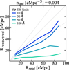 |
Fig. B.3. Median recovered bubble size versus real bubble size for 5σ Lyα equivalent width limit = [10, 30, 50, 100] Å, galaxy number density ≈0.004/cMpc3 in our asymmetry method. Gray lines from top to bottom show +30%, 0%, and +30% recover bubble size error, respectively. We can recover bubble size to within 30% error when galaxy number density is greater than 0.004/cMpc3. |
All Figures
|
Fig. 1. Cartoon illustrating the Lyα transmission profile of galaxies in a plane of the sky around an ionized bubble. Left: Galaxies in and around a spherical bubble with the observer at the top. Right: The integrated Lyα transmissions, 𝒯 as a function of transverse distance (x) measured using galaxies in the green box in the left panel. Transmission profiles 𝒯(x) viewed in different windows (A, B, and C) are different. Window A: Galaxies are all outside the bubble and all have 𝒯 ≈ 0 , resulting in a flat transmission profile in the window. Window B: Galaxies are located around the center of the bubble, therefore 𝒯 in the window are all high and the transmission profile is symmetric around the window center. Window C: Half of the galaxies are outside the bubble and have 𝒯 ≈ 0 . The other half of the galaxies are inside the bubble, having rising transmission toward the bubble center. The transmission profile around the center of window C is therefore asymmetric. The level of asymmetry can therefore be a probe of bubble edges. |
| In the text | |
|
Fig. 2. Example of an asymmetry score map made using galaxies’ Lyα transmission. Left: Simulated ionization map (4 cMpc slice from our simulation with mean neutral fraction |
| In the text | |
|
Fig. 3. Top panels: Ionization maps and galaxies colored by their Lyα transmissions, at |
| In the text | |
|
Fig. 4. Cartoon illustrating the transmission profile of galaxies along the LOS direction around a bubble. Left: Galaxies in and around a spherical bubble. Right: The integrated Lyα transmissions as a function of the LOS distance (d) measured using galaxies in the green box in the left panel. Transmission profiles (T)(z) viewed in different windows (A, B, and C) are different. Window A: Galaxies in front of the bubble are in fully neutral gas and thus experience a strong Lyα damping wing and have almost zero transmission. Stepping back into the bubble the transmission increases because of the increased path length of ionized IGM in front of galaxies. Window B: Galaxies located at the back of the bubble have the highest transmission because they have the longest path length through the ionized IGM. Window C: Galaxies on the far side of the bubble are in fully neutral IGM and have almost zero transmission. Galaxies’ integrated Lyα transmission is tightly correlated with the distance between the galaxy and the nearest neutral IGM patch along the LOS. We can use this correlation to map ionized regions along the LOS (Section 4). |
| In the text | |
|
Fig. 5. Integrated Lyα transmission as a function of the distance between a galaxy and the first neutral IGM patch the galaxy light encounters at z = 8. Solid lines in orange, maroon, and black curves show 𝒯(dIGM) for all the galaxies at |
| In the text | |
|
Fig. 6. Example sightline skewer showing galaxies’ Lyα transmissions and EW as a function of the LOS position, where the zero point of the LOS position is arbitrary. The top panel shows the ionization map in the x−z plane (white ionized, black neutral gas). Red empty and solid dots are galaxies with MUV>−17.5 in the slice. Red solid points are galaxies with fLyα>10−18 erg/s/cm2. The middle panel shows the Lyα transmission for each galaxy as a function of LOS position. Galaxies in bubbles show high transmission while galaxies in neutral IGM having transmission ≈0. Horizontal Gray lines show the spans of the simulated ionized bubbles along the sightline. Blue dashed lines are the 𝒯(dIGM) curves derived using the damping wing optical depth (Figure 5), galaxy transmissions follow this curve very well. The blue horizontal lines show the span of the recovered bubbles using our method (Section 4.1). The bottom panel shows the observed Lyα EW of the galaxies, highlighting that strong Lyα EW ≳ 50 Å likely signpost large ionized regions. |
| In the text | |
|
Fig. 7. Demonstration of our LOS-bubble-finding algorithm, where the zero point of the LOS position is arbitrary. (a) Starting from the galaxy farthest away from the observer, gi, we invert 𝒯(dIGM) (Figure 5, the red dashed line) to estimate the distance between the galaxy and the nearest neutral IGM patch, Di. We set the LOS bubble diameter, Dbubble=Di, and the redshift of the back of the bubble, zback=zi, that is, the redshift of the first galaxy. We then mark all galaxies in front of gi within Dbubble (orange dots) to be inside the same bubble as gi. (b) We then step through the bubble toward the observer to update our estimate of Dbubble. For a galaxy gi+n which is a distance di, i+n from galaxy gi we estimate the distance of galaxy gi+n from neutral IGM, Di+n. If Di+n+di, i+n>Dbubble we update Dbubble→Di+n+di, i+n. (c) Once we have iterated through all galaxies contained within Dbubble and Dbubble converges, we continue iterating through all the galaxies in the line-of-sight in the same manner to find all the bubbles. In this example sightline we find two bubbles and their associated galaxies (orange galaxies on the left and green galaxies on the right, the remaining blue point is a galaxy between the two bubbles and is not considered to be inside a bubble). |
| In the text | |
|
Fig. 8. Median recovered bubble size versus real bubble size for LOS bubbles assuming a number density of 0.004 galaxies/cMpc3 (corresponding to a complete spectroscopic sampling of galaxies down to MUV, limit=−17.2 at z≈8) for 5σ Lyα equivalent width limits = [10, 30, 50, 100] Å for the faintest galaxies (colored lines). The shaded region shows the 68% range of recovered bubble sizes for the Lyα equivalent width limit = 10 Å line. When the Lyα equivalent width limit is deeper than 50 Å we can estimate 𝒯 relatively well for each galaxy and thus we can recover bubble sizes ∼10−80 cMpc to within 30% of their true values (1−1 and 1−1±0.3 relations marked by solid gray lines). The dip at Rreal∼100 cMpc is due to sightlines that pass through a big bubble but without enough galaxies to sample the space, causing us to recover a few smaller bubbles instead of one big bubble. This could be improved in future work when 𝒯 can be more precisely estimated, for example, with a prior from the Lyα escape fraction (see Section 2.3). |
| In the text | |
|
Fig. 9. Median recovered bubble size to real bubble size ratio (Drecovered/Dreal) versus galaxy number density for 5σ Lyα equivalent limits = [10, 30, 50, 100] Å (solid lines) binned by galaxy number density. Shaded regions show the 16−84 percentile of the recovered size ratio. The method converges to the correct bubble size as we reach ≳0.004 galaxies/cMpc3. |
| In the text | |
|
Fig. 10. Mean bubble diameter as a function of |
| In the text | |
|
Fig. 11. Mean bubble diameter recovered from measuring bubbles along NLOS sightlines using our bubble mapping algorithm (Section 4), for simulations with different bubble-size distributions. The solid and shaded regions show the median and 68% range of the recovered mean bubble size from 150 realizations. With ≳15−30 sightlines it would be possible to distinguish different bubble size distributions. |
| In the text | |
|
Fig. A.1. Example of converting an asymmetry score map into a binary ionization map (top panel), and converting an ionization map into a binary ionization map (bottom panel). The left column shows the original maps. The second column shows the maps converted into binary maps by setting all the pixels with asymmetry score ( |
| In the text | |
|
Fig. A.2. Recovered bubble maps using different Athresh. From left to right column are the maps using Athresh of 0.2,0.4,0.6,0.8, respectively. When Athresh>0.5, the recovered bubbles break into too many small pieces. |
| In the text | |
|
Fig. A.3. Jaccard index for different window radius and depth combinations as a function of |
| In the text | |
|
Fig. B.1. Recovered bubble maps corresponding to different galaxy number densities ngal≈0.0040−0.0005/cMpc3 at |
| In the text | |
|
Fig. B.2. Upper panel: Input ionization map (gray neutral, white ionized) at |
| In the text | |
|
Fig. B.3. Median recovered bubble size versus real bubble size for 5σ Lyα equivalent width limit = [10, 30, 50, 100] Å, galaxy number density ≈0.004/cMpc3 in our asymmetry method. Gray lines from top to bottom show +30%, 0%, and +30% recover bubble size error, respectively. We can recover bubble size to within 30% error when galaxy number density is greater than 0.004/cMpc3. |
| In the text | |
Current usage metrics show cumulative count of Article Views (full-text article views including HTML views, PDF and ePub downloads, according to the available data) and Abstracts Views on Vision4Press platform.
Data correspond to usage on the plateform after 2015. The current usage metrics is available 48-96 hours after online publication and is updated daily on week days.
Initial download of the metrics may take a while.