| Issue |
A&A
Volume 688, August 2024
|
|
|---|---|---|
| Article Number | A106 | |
| Number of page(s) | 23 | |
| Section | Extragalactic astronomy | |
| DOI | https://doi.org/10.1051/0004-6361/202449644 | |
| Published online | 12 August 2024 | |
Peering into cosmic reionization: Lyα visibility evolution from galaxies at z = 4.5–8.5 with JWST
1
INAF – Osservatorio Astronomico di Roma, Via Frascati 33, 00078 Monteporzio Catone, Italy
e-mail: This email address is being protected from spambots. You need JavaScript enabled to view it.
2
Dipartimento di Fisica, Università di Roma Sapienza, Città Universitaria di Roma – Sapienza, Piazzale Aldo Moro, 2, 00185 Roma, Italy
3
Dipartimento di Fisica, Università di Roma Tor Vergata, Via della Ricerca Scientifica, 1, 00133 Roma, Italy
4
Department of Physics and Astronomy, Texas A&M University, College Station, TX 77843-4242, USA
5
George P. and Cynthia Woods Mitchell Institute for Fundamental Physics and Astronomy, Texas A&M University, College Station, TX 77843-4242, USA
6
Space Telescope Science Institute, 3700 San Martin Dr., Baltimore, MD 21218, USA
7
Department of Astronomy, The University of Texas at Austin, Austin, TX, USA
8
Astronomy Centre, University of Sussex, Falmer, Brighton BN1 9QH, UK
9
Institute of Space Sciences and Astronomy, University of Malta, Msida, MSD 2080, Malta
10
NSF’s National Optical-Infrared Astronomy Research Laboratory, 950 N. Cherry Ave., Tucson, AZ 85719, USA
11
Department of Physics, 196A Auditorium Road, Unit 3046, University of Connecticut, Storrs, CT 06269, USA
12
Department of Physics and Astronomy, Rutgers University, Piscataway, NJ 08854, USA
13
Departamento de Astronomía, Universidad de La Serena, Av. Juan Cisternas 1200 Norte, La Serena, Chile
14
ARAID Foundation, Centro de Estudios de Física del Cosmos de Aragón (CEFCA), Unidad Asociada al CSIC, Plaza San Juan 1, 44001 Teruel, Spain
15
Laboratory for Multiwavelength Astrophysics, School of Physics and Astronomy, Rochester Institute of Technology, 84 Lomb Memorial Drive, Rochester, NY 14623, USA
16
ESA/AURA Space Telescope Science Institute, USA
17
University of Massachusetts Amherst, 710 North Pleasant Street, Amherst, MA 01003-9305, USA
18
Department of Physics and Astronomy, University of California Riverside, 900 University Avenue, Riverside, CA 92521, USA
19
European Space Agency (ESA), European Space Astronomy Centre (ESAC), Camino Bajo del Castillo s/n, 28692 Villanueva de la Cañada, Madrid, Spain
20
Astrophysics Science Division, NASA Goddard Space Flight Center, 8800 Greenbelt Rd, Greenbelt, MD 20771, USA
21
Lawrence Berkeley National Laboratory, Berkeley, CA 94720, USA
22
Department of Physics and Astronomy, University of Louisville, Natural Science Building 102, 40292 KY, Louisville, USA
Received:
17
February
2024
Accepted:
19
April
2024
Abstract
The resonant scattering interaction between Lyα photons and neutral hydrogen implies that a partially neutral intergalactic medium has the ability to significantly impact the detectability of Lyα emission in galaxies. Thus, the redshift evolution of the Lyα equivalent width distribution of galaxies offers a key observational probe of the degree of ionization during the Epoch of Reionization (EoR). Previous in-depth investigations at z ≥ 7 were limited by ground-based instrument capabilities. We present an extensive study of the evolution of Lyα emission from galaxies at 4.5 < z < 8.5, observed as part of the CEERS and JADES surveys in the JWST NIRSpec/PRISM configuration. The sample consists of 235 galaxies in the redshift range of 4.1 < z < 9.9. We identified 65 of them as Lyα emitters. We first measured the Lyα escape fractions from Lyα to Balmer line flux ratios and explored the correlations with the inferred galaxies’ physical properties, which are similar to those found at lower redshift. We also investigated the possible connection between the escape of Lyα photons and the inferred escape fractions of LyC photons obtained from indirect indicators, finding no secure correlation. We then analyzed the redshift evolution of the Lyα emitter fraction, finding lower average values at z = 5 and 6 compared to previous ground-based observations. At z = 7, the GOODS-S results are aligned with previous findings, whereas the visibility in the EGS field appears to be enhanced. This discrepancy in Lyα visibility between the two fields could potentially be attributed to the presence of early reionized regions in the EGS. Such a broad variance is also expected in the Cosmic Dawn II radiation-hydrodynamical simulation. The average Lyα emitter fraction obtained from the CEERS+JADES data continues to increase from z = 5 to 7, ultimately declining at z = 8. This suggests a scenario in which the ending phase of the EoR is characterized by ∼1 pMpc ionized bubbles around a high fraction of moderately bright galaxies. Finally, we characterize such two ionized regions found in the EGS at z = 7.18 and z = 7.49 by estimating the radius of the ionized bubble that each of the spectroscopically-confirmed members could have created.
Key words: galaxies: evolution / galaxies: high-redshift / intergalactic medium / galaxies: ISM / dark ages / reionization / first stars
© The Authors 2024
 Open Access article, published by EDP Sciences, under the terms of the Creative Commons Attribution License (https://creativecommons.org/licenses/by/4.0), which permits unrestricted use, distribution, and reproduction in any medium, provided the original work is properly cited.
This article is published in open access under the Subscribe to Open model. This email address is being protected from spambots. You need JavaScript enabled to view it. to support open access publication.
1. Introduction
Cosmic reionization is a crucial event in the early history of the Universe, marking a transition when the intergalactic medium (IGM) changes from being largely neutral to nearly completely ionized and therefore transparent with respect to ultraviolet (UV) photons. While observations have established that reionization did indeed occurr (e.g., Fan et al. 2006; Bañados et al. 2018; Planck Collaboration VI 2020; Becker et al. 2021), the timeline’s characterization of the Epoch of Reionization (EoR) is still highly debated (e.g., Gaikwad et al. 2020; Wang et al. 2020). The Thomson electron scattering optical depth to cosmic microwave background (CMB) photons measurement (Planck Collaboration VI 2020) only provides an integral constraint of the EoR, suggesting z ∼ 7.7 as the midpoint of reionization. On the other hand, the transmitted flux in quasars (QSOs) spectra (e.g., Becker et al. 2015a; Yang et al. 2020) offers information about the ending phases of reionization, indicating that it is mostly complete by z ∼ 6, with neutral islands remaining down to z ∼ 5.2 − 5.7 (e.g., Becker et al. 2015b; Bosman et al. 2022). The paucity of known QSOs at z > 7 and the high Lyα absorption saturation for low volume-averaged neutral fractions (XHI) make it challenging to peer deeper through the EoR with QSOs.
Compared to QSOs, galaxies offer a complementary way to trace the fraction of neutral hydrogen XHI across cosmic epochs. Large-scale surveys are needed since many studies have shown that reionization is a spatially patchy process and it is subject to field-to-field variations (e.g., Castellano et al. 2016; Jung et al. 2019, 2020; Leonova et al. 2022). This picture is also supported by the latest large-volume radiation-hydrodynamics simulations of the EoR (e.g., Dawoodbhoy et al. 2018; Ocvirk et al. 2021; Ucci et al. 2021).
Currently, faint, star-forming galaxies (SFGs) are considered to be the main candidate sources that provided most of the Lyman continuum (LyC; λ < 912 Å) ionizing radiation needed to complete cosmic reionization (e.g., Robertson et al. 2013; Bouwens et al. 2015; Finkelstein et al. 2015, 2019; Livermore et al. 2017; Bhatawdekar et al. 2019; Yung et al. 2020a,b), while active galactic nuclei (AGNs) have played a minor role in the process (e.g., Giallongo et al. 2015; Hassan et al. 2018; Matsuoka et al. 2018; Parsa et al. 2018; Finkelstein et al. 2019; Kulkarni et al. 2019; Yung et al. 2021; Jiang et al. 2022; Matthee et al. 2024). In particular, Lyα- emitting galaxies (LAEs, e.g., Hu & McMahon 1996; Steidel et al. 1996) may provide our current strongest probe to study the EoR, since this line is commonly observed in high-redshift star-forming galaxies (e.g., Stark et al. 2010) and is highly sensitive to the IGM neutral content. The resonant scattering interaction between Lyα photons and neutral hydrogen causes a partially neutral IGM to heavily impact the detectability of Lyα photons (see Ouchi et al. 2020, for a review). In recent years, this effect was explored by comparing the Lyα luminosity function (LF) with the UV-continuum LF (e.g., Ota et al. 2008; Ouchi et al. 2010; Zheng et al. 2017; Itoh et al. 2018; Hu et al. 2019; Konno et al. 2018). The redshift evolution of the Lyα LF is determined by galaxy evolution and Lyα opacity of the IGM, while the UV-continuum LF is governed only by galaxy evolution. It was found that Lyα LF rapidly drops from z ∼ 6.5 to 7.5, while the UV-continuum LF experiences a milder decrease, thus suggesting an increase of XHI. A complementary approach is to measure XLyα, which is the fraction of LAEs from all of the UV continuum-selected galaxies at a given redshift. Ground-based systematic efforts have been conducted by many authors for more than a decade (e.g., Fontana et al. 2010; Stark et al. 2010; Pentericci et al. 2011, 2018a; Schenker et al. 2012, 2014; Treu et al. 2012; Caruana et al. 2014; Tilvi et al. 2014; Arrabal Haro et al. 2018; Caruana et al. 2018; Mason et al. 2019; Jung et al. 2020; Yoshioka et al. 2022) and the results show a drop of XLyα above z ∼ 6, again probing solid evidence that at higher redshifts the Universe was partially neutral. However, there is still significant scatter associated with this measurement and the precise evolution of XLyα is still debated. This is primarily caused by large statistical uncertainties associated with relatively small datasets at high redshift. Biases may be brought in by the different methods used for selecting target samples (color or photometric redshift selection), the diverse sample cuts in the UV absolute magnitude (MUV), the choice of the instrument configuration (integral field unit, slit spectroscopy, or narrow-band surveys) to identify LAEs amongst SFGs, and the limitations of using ground-based telescopes. High-redshift Lyα observations from the ground were necessarily restricted to the brightest sources (e.g., Larson et al. 2018; Harikane et al. 2019; Taylor et al. 2021) as at z > 7 Lyα moves into the near infrared (near-IR), where sky background and atmospheric telluric lines significantly limit spectroscopic sensitivity. This makes the non-detection of Lyα challenging to interpret, as it hinders the determination of the galaxy’s actual redshift. Probing the full EoR with Lyα constraints has not been fully achieved.
In this context, the advent of the James Webb Space Telescope (JWST; Gardner et al. 2006, 2023) has led to significant progress in systematically discovering galaxies at very early cosmic epochs. Early Release Science programs (e.g., Treu et al. 2022; Finkelstein et al. 2023; Bagley et al. 2024) found many high-redshift galaxy candidates at z > 9 (e.g., Castellano et al. 2022; Finkelstein et al. 2022a; Naidu et al. 2022; Adams et al. 2023; Atek et al. 2023; Bouwens et al. 2023; Harikane et al. 2023a; Casey et al. 2024). Moreover JWST/Near InfraRed Spectrograph (NIRSpec, Jakobsen et al. 2022) was shown to be successful at identifying emission lines of high-redshift galaxies (e.g., Bunker et al. 2023a; Jung et al. 2024; Roy et al. 2023; Tang et al. 2023; Jones et al. 2024; Saxena et al. 2024). Unlike ground-based telescopes, JWST can accurately measure spectroscopic redshifts using other optical or UV rest frame emission lines, regardless of whether Lyα emission is present.
In this paper, our aim is to construct a sample of high-z galaxies with robust spectroscopic redshift and completeness estimates for Lyα rest frame equivalent width, probing a wide range of redshifts throughout the EoR. We analyze data that are part of the Cosmic Evolution Early Release Science (CEERS) survey (Finkelstein et al. 2023) to select Lyα emitters and study their physical properties and the evolution of the line visibility. The paper is organized as follows. We discuss our parent sample construction in Sect. 2 and the methodology used in Sect. 3. We present the derived  and Lyα fraction XLyα measurements and discuss the correlations found within our data, in Sects. 4 and 5, respectively. We summarize our findings in Sect. 6.
In the following, we adopt the ΛCDM concordance cosmological model (H0 = 70 km s−1 Mpc−1, ΩM = 0.3, and ΩΛ = 0.7). We report all magnitudes in the AB system (Oke & Gunn 1983) and EWs to rest-frame values.
2. Data
2.1. CEERS data
In this work, we employ the publicly released JWST/NIRCam and NIRSpec data from the Cosmic Evolution Early Release Science survey (CEERS; ERS 1345, PI: S. Finkelstein). CEERS targets the CANDELS Extended Growth Strip (EGS) field (Davis et al. 2007; Grogin et al. 2011; Koekemoer et al. 2011), by observing this region in 12 pointings using the JWST/NIRSpec, NIRCam, and MIRI instruments. All the NIRCam pointings are uniformly covered in the broad band filters F115W, F150W, F200W, F277W, F356W, and F444W, along with F410M medium-band filter. Arrabal Haro et al. (in prep., see also Arrabal Haro et al. 2023a) will present the CEERS NIRSpec spectra, Finkelstein et al. (in prep., see also Finkelstein et al. 2022a,b) will discuss the target selection. For the present work, we note that only a handful of objects with previously identified redshifts were inserted in the MSA. Details on NIRCam imaging data reduction procedure are contained in Bagley et al. (2023). Photometric redshifts were obtained from version v0.51.2 of the CEERS Photometric Catalog (Finkelstein et al., in prep.) with EAZY (Brammer et al. 2008), following the methodology described in Finkelstein et al. (2023) by including new templates from Larson et al. (2023a), which improve the photometric redshift accuracy for high-z galaxies.
For this work, we only consider data obtained in the NIRSpec PRISM/CLEAR configuration, that provides continuous wavelength coverage in the 0.6−5.3 μm wavelength range. The spectral resolution R = λ/Δλ of the instrument is ∼30−300. Each pointing was observed for a total of 3107 s, divided into three exposures of 14 groups each, utilizing the NRSIRS2 readout mode. A three-point nod pattern was employed for each observation, to facilitate background subtraction. As detailed also in Arrabal Haro et al. (2023a,b), for data processing and reduction we make use of the STScI Calibration Pipeline1 version 1.8.5 and the Calibration Reference Data System (CRDS) mapping 1029, with the pipeline modules separated into three modules. In brief, the CALWEBB_DETECTOR1 module addresses detector 1/f noise, subtracts dark current and bias, and generates count-rate maps (CRMs) from the uncalibrated images. The CALWEBB_SPEC2 module creates two-dimensional (2D) cutouts of the slitlets, corrects for flat-fielding, performs background subtraction using the three-nod pattern, executes photometric and wavelength calibrations, and resamples the 2D spectra to correct distortions of the spectral trace. The CALWEBB_SPEC3 module combines images from the three nods, utilizing customized extraction apertures to extract the one-dimensional (1D) spectra. Finally, both the 2D and 1D spectra are simultaneously examined with the MOSVIZ visualization tool (Developers et al. 2023) to mask potential remaining hot pixels and artifacts in the spectra. After masking image artifacts, data from three consecutive exposure sequences are combined to produce the final 2D and 1D spectral products. Arrabal Haro et al. (in prep.) will present a more detailed description of the CEERS NIRSpec data reduction.
We did not consider PRISM NIRSpec data observed in pointings 9 and 10, since (due to a short circuit issue) they are contaminated and lack secure flux calibrations. To investigate potential residual issues in the absolute flux calibration caused by slit losses (although CALWEBB_SPEC2 step of the pipeline already employs a slit path loss correction) or other inaccuracies in flux calibration files, as a first step, we checked the consistency with the broad band photometry by integrating the spectra across the NIRCam filter bandpasses. We then compared this synthetic photometry with the measured NIRCam photometry. From this procedure, we obtained the correction factors for the spectra in each NIRCam filter. For the high-redshift sample we consider in this work, the multiplicative flux correction factors have an average value of ∼1.4, in agreement to the values found by Arrabal Haro et al. (2023b). Most importantly, we find that these corrections remain constant across wavelength. Given that in this paper we will deal with EWs and line flux ratios, we consider the spectra derived by the standard pipeline, without applying any further corrections. The only exception is the MUV calculation (see Sect. 3.2).
In our analysis, we also consider HST photometry, in the F606W, F814W, F125W, F140W, and F160W filters, which are presented in the official EGS photometric catalog (see Stefanon et al. 2017). In the following section, we provide a brief summary of our sample selection criteria.
2.2. CEERS Parent sample selection
For our purposes, we needed to assemble the largest possible sample of high redshift sources with secure spectroscopic redshifts, whose spectra contain information about the Lyα line within the observed wavelength range. The range covered by the PRISM/CLEAR configuration sets a lower limit of z ∼ 4 on the range where we would be able to probe Lyα emission. We therefore selected all the sources with a photometric redshift higher than 3 (to allow for even large photometric redshift uncertainties) and visually examined the 2D and 1D spectra simultaneously in order to derive a spectroscopic redshift. This was done by searching for the relatively bright optical lines (e.g., [O III]λλ4959,5007, [O II]λλ3727,3729, Balmer lines, [S II]λλ6716,6731, and [S III]λ9531) and the Ly-break feature, as a whole set. We report some examples in Fig. 1, covering the redshift range probed. We determined spectroscopic redshifts for 281 galaxies out of 343 inspected sources, achieving an 82% success rate, based on the peak of the emission line with the highest signal-to-noise ratio (S/N). Among these, 150 galaxies are at z > 4.1 and include Lyα line spectral information in the observed wavelength range. In the following, we will refer to the latter as our parent sample. While the above method is slightly less precise compared to a multiple line fitting procedure, the spectroscopic redshifts derived were independently reviewed by other team members, with no questionable cases. Additionally, for galaxies with previously published spectroscopic redshifts, there is good consistency between these values and our estimates up to the second decimal place. Specifically there are 27 galaxies in common with Chen et al. (2024), 10 with Davis et al. (2023), 7 with Harikane et al. (2023b), 1 with Jung et al. (2024), 2 with Kocevski et al. (2023), 45 with Mascia et al. (2024), 118 with Nakajima et al. (2023), 15 with Nakane et al. (2024), and 10 with Tang et al. (2023). In all cases, our spectroscopic redshifts are consistent with those reported in the literature, up to the second decimal place. We note that some CEERS high-z sources might be absent from our sample due to the initial photometric redshift selection criteria, since we did not visually inspect all the PRISM spectra. Arrabal Haro et al. (in prep.) will present the complete catalog of spectroscopically-confirmed sources in CEERS.
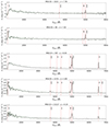 |
Fig. 1. 1D spectra examples from the parent sample. Back solid line and green shaded region represent the flux and associated error respectively. For each galaxy, we report the emission line features spotted for the identification of the spectroscopic redshift. The position of the Lyα line is also highlighted. MSA ID = 44 and 1374 are Lyα emitters with S/N > 3, while MSA ID = 1023, 397, and 11 117 have no Lyα in emission. We report wavelengths in the rest-frame for clarity. |
In Figs. 2 and 3, we present the redshift and spatial distributions respectively of all the CEERS galaxies in the parent sample (150 sources). In Table 1, we report our spectroscopic redshift measurements for the Lyα emitting galaxies subset (50 galaxies with a positive Lyα flux detection, see Sect. 3.1), together with spectroscopic and physical properties, derived as detailed in the following sections.
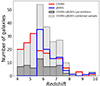 |
Fig. 2. Redshift distribution of the 150 sources (AGNs included) identified in CEERS and of the 91 galaxies presented in Jones et al. (2024) from the JADES survey. Lyα emitting galaxies with S/N > 3 from the combined sample are shown in dark grey. |
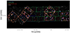 |
Fig. 3. Spatial distribution of the 150 sources (AGNs included) spectroscopically-confirmed in CEERS. Blue (red) dots are galaxies that do (do not) show Lyα emission with S/N > 3. The AGNs are represented by the yellow dots. Green and orange squares represent the pointings for NIRCam and NIRSpec, respectively. The HST and JWST images of the field are shown in the background. |
Physical and spectroscopic properties of the Lyα emitting galaxies in the CEERS sample.
2.3. CEERS AGN identification
JWST has identified an unexpected number of AGNs at high redshift (e.g., Harikane et al. 2023b; Maiolino et al. 2023; Matthee et al. 2024). From our follow-up analysis, we needed to exclude possible AGNs from our parent sample, since the mechanisms that allow Lyα to escape from an AGN are different than in galaxies and the presence of even a few such objects might bias the measurement of the line visibility statistics. In addition, since we also aimed to derive the physical properties of our sources through standard SED fitting, a treatment of AGN would require ad hoc templates which we do not include in our tool (ZPHOTFontana et al. 2000, see Sect. 3.3).
To exclude AGNs from the parent sample, we first visually examined all the spectra to search for any high-ionization emission lines (such as C IVλ1550) in the NIRSpec PRISM/CLEAR configuration. Whenever available, we also inspected the NIRSpec medium-resolution (R ≈ 1000) grating (G140M/F100LP, G235M/F170LP, and G395M/F290LP) observation for the same sources, to search for typical broad optical emission lines, which would be difficult to identify using the PRISM, due to the low resolution. We are limited in this procedure, since only 55 sources in the parent sample have a grating observation as well. We identified five AGNs following the described procedure, namely, source MSA ID = 2782 which shows broad Hα (Kocevski et al. 2023) and bright C IVλ1550; MSA ID = 746 which has broad Hα (Kocevski et al. 2023; Harikane et al. 2023b); MSA ID = 1244 which has broad Hα (Harikane et al. 2023b) and bright C III]λ1908; MSA ID = 80457 a new “candidate” AGN that reveals broad Hα; MSA ID = 82294 which shows bright C IVλ1550. We also added MSA ID = 1665 (not flagged from our visual inspection) to the AGN list, given the high Akaike information criterion (AIC) score (see Harikane et al. 2023b, for more details).
We finally checked the X-ray emission from the sources in our parent sample using the AEGIS-X Deep (AEGIS-XD) survey’s catalog (Nandra et al. 2015). Due to the relatively shallow flux limit probed by these observations, we do not find any X-ray sources that match with our parent sample. In conclusion, from the 150 sources in the parent sample we find 6 AGNs in total that are excluded from any further analysis. Therefore, the CEERS sample consists of 144 galaxies at 4.1 < z < 9.8.
2.4. JADES data
We include in our study all data presented in Jones et al. (2024) which were observed with the same NIRSpec PRISM/CLEAR configuration as the CEERS sources. These data come from the JWST Advance Deep Extragalactic Survey (JADES DR1; Bunker et al. 2020, 2023b; Eisenstein et al. 2023) targeting the GOODS (The Great Observatories Origins Deep Survey; Giavalisco et al. 2004) north and south fields.
Jones et al. (2024) presented the IDs, coordinates, spectroscopic redshifts, and spectroscopic properties of GOODS-South sources. In total they report 15 galaxies with a detected Lyα emission (5.6 < z < 7.3) in the NIRSpec PRISM/CLEAR configuration and 76 non-emitters (5.6 < z < 9.9). Saxena et al. (2024) provides the UV-β slopes, and the Lyα escape fraction measurements for 11 of the above emitters, while Rieke et al. (2023) presents catalogs with photometry and half-light radii information. To exclude possible AGNs from this sample, we checked the flags given by Luo et al. (2017) for the GOODS-South field. No matches were found, so we proceed under the assumption that the sample, which we will hence refer to as the JADES sample throughout this study, does not contain any AGNs.
In Fig. 2, we present the redshift distribution of the entire sample from CEERS (144 galaxies) and JADES (91 galaxies), which consists of 235 galaxies in the redshift range 4.1 < z < 9.9 with homogeneous JWST NIRSpec PRISM/CLEAR data selected through photometric redshifts.
3. Methods
3.1. Lyα emission line measurements
The method employed to extract the Lyα line information from the CEERS sample is similar to the one adopted by Jones et al. (2024). In this section, we give a brief description of the main points followed in our analysis.
For each source, we considered the spectroscopic redshift identified (see Sect. 2.2) to fit the emission region of the spectrum where Lyα is in the observed frame (∼4−5 pixels). The low resolution of the PRISM requires fitting models that account for both the Lyα emission line and the adjacent continua. The red continuum (λ > 1216 Å) was derived by directly fitting a linear function to the data, weighed for the inverse of their flux error from the spectrum. The wavelength range considered for the linear fit spans from 1900 Å rest-frame to the closest pixel red-ward of the Lyα emission (∼3 pixels from the peak), to avoid the possible presence of the C III]λ1908 emission line. The blue continuum (λ < 1216 Å) is expected to vary depending on the neutral hydrogen absorption and it is dependent on the redshift of the source. Thus, it was obtained by averaging the flux blue-ward of the emission line. We then defined a modified step model, whose flux is equal to the constant blue continuum value where λ < (1 + z)×1216 Å and to the red continuum values obtained by the linear fit for λ ≥ (1 + z)×1216 Å.
The low resolution of the PRISM configuration prevents us from characterizing an asymmetric Lyα profile. We thus decided to fit each line emission with a library of Gaussian profile models, as detailed below. Because of the scattering nature of the Lyα line, the peak of the emission is often slightly shifted from the systemic value, up to few hundred km s−1 (e.g., Steidel et al. 2010; Verhamme et al. 2018; Marchi et al. 2019), so we fixed the mean of the Gaussian models to the observed emission peak rather than the systemic redshift. The other two parameters of the Gaussian profiles were constrained to be within the following ranges: the FWHM ∈ [100, 1500] km s−1 and the peak amplitude ∈[0.01, 10]×10−18 erg s−1 cm−2 Å−1.
We then added the modified step model to the library of Gaussians and convolved the result with a Gaussian kernel, whose standard deviation is defined as σR(λ)[Å] = 1216(1+z)/2.355 R(λ). The convolution is applied to mimic the resolution of the instrument R(λ) at the peak of the Lyα emission in the observed frame. R(λ) is provided by the JWST documentation2 with the assumption of a source that illuminates the slit uniformly. The resulting models were also re-sampled at the finite set of wavelengths observed in the real spectra. As a final step, we employed EMCEE (Foreman-Mackey et al. 2013) to perform a Markov chain Monte Carlo (MCMC) analysis for each target spectrum, identifying the best-fitting model free parameters. The best model parameters and the integrated Lyα flux from the intrinsic emission line Gaussian model are determined through the posterior distributions resulting from the MCMC fitting routine. Uncertainties are calculated based on the 68th percentile highest posterior density intervals. We derive the S/N from the integrated Lyα flux. The rest-frame Lyα equivalent width (EW0) is computed based on the integrated Lyα flux, taking into account both the continuum flux determined at the Lyα line’s position from the red continuum fit and the spectroscopic redshift. In Fig. 4, we provide a few examples of the results obtained from the described fitting procedure for a range of emission line S/N.
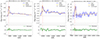 |
Fig. 4. Several examples of fitted Lyα emitters in the sample for different values of the emission line S/N. Left: MSA ID = 1561 with S/N = 23; Center: MSA ID = 439 with S/N = 7; Right: MSA ID = 1142 S/N = 3. In the upper panels, the blue solid line and shaded area denote the flux and error measurement as a function of the observed wavelength. The best fit-model is represented by an orange solid line, with the related |

The measurement of rest frame Lyα equivalent width is challenging and careful modeling is needed to recover it, due to the low resolution at the blue end of the NIRSpec/PRISM instrument. To further prove this point, for each source we extracted again the EW0 by directly integrating the continuum-subtracted line profile over the same emission region of the spectrum (∼4−5 pixels centered on the emission peak). We consistently obtained lower values, which are smaller by 30% on average than the reference results from our modeling. This effect was also noted by Chen et al. (2024), who report potential underestimation from direct integration by as much as 30%–50%. This is indeed expected in the case in which a fraction of the Lyα photons fall on pixels dominated by the continuum and break.
We expect the shift of the Lyα emission line compared to the systemic redshift to be typically below 1 pixel (Δv < 2500 km s−1 given the PRISM dispersion at these wavelengths). This is indeed true in all cases except for four galaxies which show shifts up to 2 pixels (MSA ID = 1420, 2089, 2168, and 80445). The identified lines could be the unresolved [N V]λλ1239,1243 instead of Lyα (although it would be the only sign of AGN emission) or a spurious detection. However, we are aware that there could be residual issues with the wavelength calibration of the spectra, due to the highly variable spectral resolution of the PRISM which have also been observed in other spectra, with discrepancies between red and blue regions. For this reason, we decided to keep the four objects in the Lyα list.
In total we found 50 CEERS Lyα emitting galaxies (of those, there are 43 with S/N > 3 and 7 that are tentative emitters with 2 < S/N < 3), whose properties are reported in Table 1, whereas 94 galaxies have no Lyα emission. In the appendix (see Appendix A) we show all the Lyα line profiles fitted (including the tentative ones). In Fig. 5, we show the distribution of the measured EW0 for CEERS, together with the published JADES data (Jones et al. 2024), for a total of 65 Lyα emitting galaxies in the redshift range of 4.2 < z < 7.8. For all sources (including those where Lyα is not detected), we also derive a limit on the lowest EW0 that could be measured given the spectroscopic redshift (z), the red continuum value next to Lyα ( ), and the flux error at the observed Lyα peak of the spectrum (E(λLyα)), adopting Eq. (2) from Jones et al. (2024):
 (1)
(1)
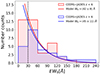 |
Fig. 5. EW0 distribution of the Lyα emitting galaxies in the combined CEERS + JADES sample. The red (blue) histogram shows the population at z < 6 (z > 6). The red (blue) solid line shows the best fit exponential declining distribution P(EW)∝e−EW0/W0 using EMCEE (Foreman-Mackey et al. 2013). The two populations are sampled in the range −21 < MUV < −17. |
where the numerator stands for the integrated flux of a Gaussian, whose amplitude and standard deviation equal to the flux error at the observed Lyα peak of the spectrum E(λLyα) and to the Gaussian kernel, σR, that accounts for the instrument resolution, respectively. We find EW0, lim values from a few Å to 155 Å, with a median of 11 Å.
As a final check, we inspected the grating spectra of all galaxies when available. Of the 29 galaxies at z > 6.98 (where Lyα emission is in the detectable range of G140M/F100LP), 6 have medium-resolution observations. One (MSA ID = 20) is a tentative emitter according to the PRISM measurement, but does not show Lyα in the grating spectrum. The other five are non-emitters according to the PRISM observations; of these, only one (MSA ID = 1027) shows a faint Lyα line in the medium resolution spectrum, whose EW0 (Larson et al. 2022; Tang et al. 2023) is below the PRISM detection limit.
3.2. MUV and β
We calculated the UV absolute magnitudes (MUV) directly from the observed PRISM spectra, after correcting them for the ×1.4 average factor already discussed in Sect. 2.1 to match the photometry. We used this average factor for the whole sample, since for 45 galaxies in the sample, we do not have individual NIRCam photometry. We measured the median flux density and error within the rest-frame 1400−1500 Å range to compute the UV absolute magnitudes (to be consistent with the values reported in Jones et al. 2024 for the JADES data). In Fig. 6 we report the relation between the measured EW0 and MUV. As expected for the fainter galaxies, we were only able to measure the Lyα emission for higher EW0 due to the flux limited nature of the spectroscopic observations. The data from Jones et al. (2024) are reported in grey for a direct comparison.
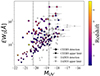 |
Fig. 6. Lyα EW0 versus MUV for our sample. Circles denote measured EW0 with S/N > 3, while triangles represent galaxies with just EW0, lim upper limits. CEERS data are color coded by redshift, while JADES galaxies are reported in grey for comparison. The black dashed lines (MUV = −20.25 and −18.75) divide the sample from the bright and faint ends. |
The UV-β slopes were measured as in Mascia et al. (2024) and Calabrò et al. (2021) by employing all the photometric bands whose bandwidth ranges fall between 1216−3000 Å rest-frame. The former limit is set to exclude the Lyman-break. We then fitted the available photometric bands amongst HST F814W, F125W, F140W, F160W and JWST-NIRCam F115W, F150W, or F200W data (see Sect. 2), depending on the exact redshift of the sources and the accessibility of data. Notably, 16 out of the 56 emitters in the CEERS parent sample lack JWST-NIRCam data, therefore we are limited to consider the HST bands for fitting these sources. We fitted a single power-law of the form f(λ) ∝ λβ (Calzetti et al. 1994; Meurer et al. 1999). Typically we employed between 2 and 4 bands. For each galaxy, the measured β and its uncertainty are obtained as the mean and standard deviation of a n = 1000 Monte Carlo approach, through which fluxes in each band are extracted according to their error.
3.3. Measurements of physical properties
Physical properties were derived following the method described in Santini et al. (2022), fixing the redshift of each source to the spectroscopic value. We measured the stellar mass (mass), star formation rates (SFR) and dust reddening (E(B − V)) by fitting synthetic stellar templates with the SED fitting code ZPHOT (Fontana et al. 2000). For the fit, we used the seven-band NIRCam photometry of the sources combined to the HST photometry, if both available. Otherwise, for the 16 emitters that do not have NIRCam photometry (see Sect. 2), only HST photometry was used. In this case, the derived stellar masses have higher uncertainties and are slightly biased to higher values (we defer a more exhaustive discussion of this issue to Calabró et al., in prep.). We fit the observed photometry (see Sect. 2), adopting Bruzual & Charlot (2003) models, the Chabrier (2003) IMF and assuming delayed star formation histories (SFH(t) ∝ (t2/τ)⋅exp(−t/τ)), with τ ranging from 100 Myr to 7 Gyr. The age could vary between 10 Myr and the age of the Universe at each galaxy redshift, with assumed metallicity values of 0.02, 0.2, 1, or 2.5 times solar metallicity. For the dust extinction, we used the Calzetti et al. (2000) law with E(B − V) ranging from 0 to 1.1. Nebular emission was included following the prescriptions of Castellano et al. (2014) and Schaerer & de Barros (2009) and assuming a null LyC escape fraction.
We used the same method to measure stellar mass, SFR, and E(B − V) from the 15 emitters from the Jones et al. (2024) sample. We employed the published Rieke et al. (2023) photometric catalog for this purpose. Total fluxes in all bands were obtained multiplying the reported fluxes and uncertainties in fixed circular apertures of 0.15″ (corresponding to ∼2 FWHM in F444W), computed on point spread function-matched (PSF-matched) images, with the scaling factor given by the ratio of the total (Kron) flux and the aperture flux in the detection band (see, e.g., Merlin et al. 2022).
The MUV and UV-β slopes for our Lyα emitting galaxies are reported in Table 1. For the JADES subset, Jones et al. (2024) provide MUV for all galaxies, while Saxena et al. (2024) provide UV-β slopes for 11 out of 15 emitters.
3.4. Optical line flux measurements and dust correction
We measured the total flux of each detected Hα, Hβ, [O III]λλ4959,5007, and [O II]λλ3727,3729 with a single Gaussian fit. Given the resolution of the instrument the [O II]λλ3727,3729 is unresolved and we treat it as a single feature. For this part of our analysis we followed the same procedure as described in Mascia et al. (2024), using MPFIT code3 (Markwardt 2009). For Hβ, we also derived rest-frame equivalent width values.
Limited by the wavelength coverage of the NIRSpec PRISM configuration, a direct dust correction estimate is not available for each target by considering only the Hα/Hβ Balmer ratio. For this reason, we adopted dust attenuation based on the Balmer decrement when Hα/Hβ is observed and the gas reddening values provided by the SED fitting otherwise (see Sect. 3.3). As reported in Osterbrock & Ferland (2006), we consider the intrinsic Hα/Hβ ratios to be 2.86 by assuming case B recombination with a density ne = 100 cm−3 and temperature Te = 10 000 K. Then we corrected Hα and Hβ fluxes by dust extinction using the reddening curve values provided by Calzetti et al. (2000).
We also employed the O32 line ratios in Mascia et al. (2024). We considered the O32 values provided by Saxena et al. (2024) for 11 out of 15 emitters in JADES.
3.5. UV half-light radius measurements
We measured the half-light radius re of each galaxy in the rest-frame UV using the same procedure adopted by Mascia et al. (2024), with the python software GALIGHT4 (Ding et al. 2020). The latter adopts a forward-modeling technique to fit a model to the observed luminosity profile of a source. We assume that galaxies are well represented by a Sérsic profile, constraining the axial ratio q to the range 0.1 − 1 and the Sérsic index n to 1, which has been shown to be the best suitable choice for high-z star forming galaxies (e.g., Hayes et al. 2014; Holwerda et al. 2015; Morishita et al. 2018; Yang et al. 2022), and also for the CEERS sources, as detailed in Mascia et al. (2024). We remark also that LAEs tend to be more compact in their UV emission than the general population of lyman-break galaxies (LBGs), as recently shown by Napolitano et al. (2023) and Ning et al. (2024). We visually checked from residuals that the luminosity profiles were well fitted by the Sérsic function. The fit was performed in the F150W (F115W) NIRCam images for all sources at z > 5.5 (z < 5.5) to ensure the best homogeneity in the rest-frame range. For the 14 sources that do not have NIRCam photometry, HST-WFC3 observations in the F160W (F125W) were used for the two redshift ranges. For unresolved sources we place an upper limit. The values are reported in Table 1. More information about both the procedure and the justifications for these assumptions can be found in Mascia et al. (2024), where we also briefly describe the simulations implemented to determine the minimum measurable radius in the various bands.
For the JADES subset, since all galaxies are at z > 5.5 (see Fig. 2) we consider the half-light radii obtained from F150W photometry (see Rieke et al. 2023, for further details). Only 10 out of the 15 emitters found by Jones et al. (2024), have a half-light radius measurements in the published catalog.
4. Properties of Lyα emitting galaxies
In this section, we further analyze the derived properties of the combined sample of Lyα emitting galaxies, from both CEERS (50 galaxies) and JADES (15 galaxies), for a total of 65 galaxies in the redshift range 4.2 < z < 7.8.
4.1.
 measurement
We estimated  as the ratio between the observed Lyα emission flux measured in Sect. 3.1 and the expected intrinsic Lyα emission flux calculated from the detected Balmer emission lines. For the intrinsic Lyα emission flux, we adopted Case B recombination, assuming a density of ne = 100 cm−3 and temperature of Te = 10 000 K. As reported in Osterbrock & Ferland (2006), we considered the intrinsic Lyα/Hα and Hα/Hβ ratios to be 8.2 and 2.86 respectively. Modifying these assumptions within the typical range for star-forming regions (5000 K < Te < 30 000 K and 10 cm−3 < ne < 500 cm−3) results only in a few percent change in the above ratios (e.g., Sandles et al. 2023; Chen et al. 2024).
To derive  for our 50 Lyα emitting galaxies (see Table 1), we only considered fluxes measured from PRISM/CLEAR configuration spectra (see Sects. 3.1 and 3.4). We used the measured Hα flux whenever it is observed in the spectral range (30 galaxies); otherwise, we used the Hβ flux (14 galaxies). For five galaxies with HβS/N < 3, we could only derive lower limits on
  . For one emitter (MSA ID = 82372), we could not measure the
  or an upper limit, due to lack of both Hα and Hβ in the spectra covered by our observations. In Table 1 we report the
  value with the uncertainty derived by propagating the error of Lyα and Balmer fluxes. The median value for the sample is 0.13, but the values span all the way to ∼0.8. To attain such a high
  , it might be necessary for the nearest predominantly neutral IGM patch to be situated at a distance of at least 1−2 physical Mpc (pMpc). We discuss this further in Sects. 5.3 and 5.4.
4.2. Correlations between  and physical properties
In this section, we further investigate the dependencies between the Lyα escape fraction and the physical properties of the emitters. In Fig. 7 we present the correlations we found between  and EW0, the stellar mass, UV absolute magnitude, reddening, UV slope β, and SFR of all the CEERS and JADES emitters derived in Sect. 3. To quantify the existence of correlations, we ran a Spearman rank test between
  and the derived properties. Whenever lower limits were present, we used these values multiplied by
  . We considered a correlation to be present whenever the p-value is p(rs) < 0.01 (see Table 2). As expected, the strongest correlations are with the EW0 and MUV, and the strongest anti-correlations are with the Mass and the E(B − V). As noted by Saxena et al. (2024), since by definition
  and EW0 are both calculated from the observed Lyα flux, the observed strong correlation between
  and EW0 implies that the Hα (or Hβ) flux does not scale with Lyα. Also Roy et al. (2023) and Begley et al. (2024) report the same trend from intermediate redshift emitters, respectively from GLASS and VANDELS data. The interpretation of the correlation between
  and MUV is two-fold.
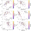 |
Fig. 7. Lyα escape fraction as a function of rest frame Lyα equivalent width, stellar mass, UV absolute magnitude, reddening, UV β slope, and star formation rate. CEERS and JADES data are represented by circles and diamonds respectively. We report lower limits with black arrows, error bars are in grey instead. In the top-left panel, we show the fit relation found by Begley et al. (2024) in VANDELS z ∼ 4 − 5 data. In the middle-right panel, we show the best fitting relations found by Hayes et al. (2011), which exhibit a slight deviation from the trend proposed by Calzetti et al. (2000). |
Spearman correlation coefficients with the Lyα escape fraction for the Lyα emitting galaxies sample.
On the one hand (as already discussed in Sect. 3.2 for the faint population), this is produced by the flux limited nature of spectroscopic observations. However, the fact that we do not observe high  from the UV-bright population is a real effect, and suggests an increasing neutral gas fraction and dust in more luminous galaxies. This result, also in agreement with Saxena et al. (2024), is supported by the anti-correlation we find with stellar mass. UV bright massive systems are likely to have an increasing neutral hydrogen content in their interstellar media (ISM), which due to the resonant scattering nature of Lyα (for a review, see Dijkstra 2017) attenuates its emission along the line of sight, because the probability of the Lyα photons to be absorbed by dust also increases (Verhamme et al. 2015; Gurung-López et al. 2022). The key role of dust in the process is also highlighted by the typical steep UV β slopes (Lin et al. 2024), low reddening and low star formation rates values we find for the galaxies with the highest values of
  . We report in Fig. 7 the best-fitting relation identified by Hayes et al. (2011) between
  and reddening. This trend differs slightly from the dust attenuation model proposed by Calzetti et al. (2000), as it enforces
  for a zero value of E(B − V). Finally we find only a marginal anti-correlation between the
  and re, which is consistent with the compact of Lyα emitters as already described in Napolitano et al. (2023). However the p-values are higher than the threshold and cannot be considered to be conclusive. All the above trends were known to exist at lower redshift: our results indicate that the nature of LAEs and the mechanisms that favour the line visibility do not change much with redshift and seem to be still primarily associated with the galaxies physical properties. If confirmed with larger samples of Lyα emitters at z > 7, this could imply that the role of the IGM in suppressing Lyα visibility is more likely an on/off effect, with lines of sight that are almost free for the Lyα photons to escape unattenuated and others where the Lyα is completely absorbed (similar to the simple number evolution scenario suggested by Tilvi et al. 2014). The inhomogeneity of reionization will be discussed further in Sect. 5.3.
4.3. Lyman continuum escape in Lyα emitters
A direct detection of the Lyman continuum (LyC) emission escaping from the high-z galaxies is not possible given the extremely high opacity of the IGM to LyC photons at z > 4.5 (Inoue et al. 2014). However it is essential to estimate this quantity to understand the nature of galaxies contributed mostly to the reionization process. Recently, several authors (e.g., Chisholm et al. 2022; Roy et al. 2023; Saxena et al. 2024) tackled this problem by deriving empirical relations that connect key physical or observational properties to the escape of LyC photons of galaxies. The relations are either derived from simulations (e.g., Choustikov et al. 2024) or from the samples of low redshift LyC emitters for which detailed derivation of the physical properties are available (Flury et al. 2022). In this context, in Mascia et al. (2023, 2024) we developed two empirical relations that predict  from a set of photometric and spectroscopic indirect indicators, identified in the most complete low-redshift sample of Lyman continuum emitters (see Flury et al. 2022), namely the O32 ratio, the UV radius re, and the UV β slope (or in alternative EW(Hβ), the UV radius re, and β – see the above paper for more details and a comparison between the two methods). Similarly Chisholm et al. (2022) developed an empirical relation that is based on just the UV β slope to obtain a predicted LyC escape fraction. We employed the relation based on O32, re, and β for the 41 sources in the CEERS Lyα emitters sample for which O32 is measurable, and the EW(Hβ), re, and β relation for the remaining 9 CEERS Lyα emitters for which O32 is not available. We note that there are nine unresolved sources for which re is given as an upper limit (see Sect. 3.5): in these cases, given the anti-correlation between re and
  , the derived
  are the lower limits. In Table 1, we report the obtained values.
For the JADES sample, we could only calculate the predicted LyC escape fraction for 10 emitters for which the values of O32, re, and β are reported in the literature (see Sect. 3.5).
In Fig. 8, we show the relation between the inferred  and the
  . The left panel includes all post-reionization galaxies (z < 5.5), while the right panel only shows galaxies that reside in a partially ionized IGM. Since Lyα is known to correlate with the
  in the local universe and at z = 3 (e.g., Marchi et al. 2017; Gazagnes et al. 2020; Pahl et al. 2021), given that the photons can escape through common clear channels in the ISM (e.g., Verhamme et al. 2015; Dijkstra et al. 2016; Jaskot et al. 2019), we would expect to see a correlation between the two quantities at z ∼ 4.5 − 5.5. On the other hand, when galaxies start to be surrounded by a partially neutral IGM, such a correlation could be lost, as the Lyα visibility is no more driven by the galaxies properties alone, but also by the local IGM conditions. Saxena et al. (2024) and Mascia et al. (2024) already noted the absence of any correlation in their more limited samples, with Saxena et al. (2024) also noting that the predicted LyC escape fraction is always lower than the Lyα escape fraction. We do not see evidence for this effect, as many galaxies considered in this work actually have higher inferred LyC escape. We also note that the best fitting relation (
 ) found by Begley et al. (2024) from the analysis of the interstellar absorption lines in stacked spectra at z ∼ 4 − 5 from VANDELS data predicts lower values of
  than what we obtain in this work.
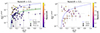 |
Fig. 8. Lyα escape fraction as a function of the LyC escape fraction inferred from the combination of spectroscopic properties using the relation derived by Mascia et al. (2024). Symbols are the same as in Fig. 7. The left panel includes all post-reionization galaxies (z < 5.5) while the right panel includes galaxies residing in a partially ionized IGM. For comparison, we report with the solid green line and region the best fitting relation found by Begley et al. (2024) for z ∼ 4 − 5 emitters. |
Contrary to our expectations, we do not find any secure correlations at either redshift ranges, although admittedly the lower redshift sample is rather small (24 galaxies) and the uncertainties on the inferred LyC escape fractions are significant. The sample at z < 5.5 (z > 5.5) has a Spearman coefficient of 0.29 (0.16) with a p-value = 0.16 (0.36). We note however that the average  of Lyα emitting galaxies, is 0.16, that is: slightly higher than what reported by Mascia et al. (2024) for the general LBG population with similar MUV.
For completeness, we also used the Chisholm et al. (2022) relation to derive alternative  values, but imposing a maximum of
  for galaxies with extremely blue colors. On average, these values are lower than the one derived with our relations, but they also do not seem to correlate with the
  .
.
5. Evolution of the Lyα visibility during reionization
During the epoch of reionization, the visibility of Lyα emission in galaxies is due to the combination of the physical properties of the galaxies that regulate how many photons can emerge from a galaxy through the interstellar and circumgalactic media, and of the conditions of the surrounding IGM, whose neutral fraction XHI determines the number of Lyα photons that are expected to reach us. To take into account the first factor people usually employ MUV matched samples and rely on the fact that the typical timescales for galaxy evolution at very high redshift are relatively short (e.g., there are only 170 Myr between z ∼ 6 and z ∼ 7). Thus, any remaining effect on the Lyα visibility above z ∼ 6 is attributed to a changing neutral fraction in the IGM (e.g., Mason et al. 2018a; Pentericci et al. 2018b). In other words, the z ∼ 6 universe is usually assumed to be completely ionized and, thus, the Lyα visibility at this epoch is used as the benchmark to compare its evolution. This view has been recently questioned by the discovery of significant fluctuations in the HI optical depth in QSO spectra and the presence of extended regions of high opacity down to z ≃ 5.3 which suggest an extended final phase and a late end of hydrogen reionization (Zhu et al. 2023; Bosman et al. 2022). Crucially, the CEERS sample that we are presenting in this work covers observations of Lyα emission at z > 4.5 and we are thus able to assemble a solid baseline sample of Lyα measurements in the post-reionization epoch, that is, where no more neutral islands exist. Also contrary to previous works, this baseline post-reionization sample is observed with the same configuration as the reionization sample, while previous analyses compared z ∼ 6 EW0 distribution typically obtained by optical instruments (Schenker et al. 2012; De Barros et al. 2017) to observations at z > 7 obtained with near-IR spectrographs (Mason et al. 2018a; Jung et al. 2022). In the following section, we will compute the Lyα fractions from the CEERS and JADES samples.
5.1. Evolution of the Lyα emitter fractions
We define the Lyα emitter fractions as the number of galaxies with a measured Lyα emission with EW0 > 25 Å (or > 50 Å) over the total number of galaxies, in four redshift bins, centered at z = 5, 6, 7, and 8 and with Δz = 1. We only include in our calculations all galaxies in the range −20.25 < MUV < −18.75 to be consistent with most previous works, which used these values to separate bright and faint galaxies following the very first studies (Stark et al. 2011; Pentericci et al. 2011; Ono et al. 2012). A large fraction of the CEERS galaxies belong to this magnitude range (see Fig. 6), with only a few sources having brighter or fainter magnitudes; whereas JADES has a higher number of sources fainter than MUV = −18.75. For all sources, we take into account the rest frame EW limit (EW0, lim) that identifies the minimum rest-frame equivalent width we could possibly detect given their redshift and continuum flux. This is to avoid biasing the derived visibilities, e.g., bright Lyα emission lines detected in relatively shallow data could bias the derived visibility upwards, while the inclusion of many undetected sources for which we could not in any case detect Lyα would bias the fraction down. We note that 115/235 galaxies, namely, ∼49% (131/235 galaxies, i.e., ∼56%) of data in the parent sample fulfills both the MUV cut and EW0, lim < 25 Å (< 50 Å) requirements. The results for the two different values of Lyα EW are presented in Fig. 9 for the entire redshift range. We show the results for the CEERS and JADES samples separately, and for their combination. For JADES only the bins at z ≥ 6 are populated. Given the low number of detections in each bin, the uncertainties are evaluated using the statistics for small numbers of events developed by Gehrels (1986). We can see that while at z = 6 the JADES and CEERS fractions are in perfect agreement for both EW limits, at higher redshifts, there is a very large discrepancy between the two fields. At z = 7, for the EGS field we derived a much higher fraction, which might be due in part to the presence of three Lyα emitters around z = 7.18 and three emitters around z = 7.49. We will discuss both structures in Sects. 5.3 and 5.4, respectively. We note that in the CEERS field another overdensity has been previously identified at z = 7.7 by Tilvi et al. (2020), Jung et al. (2022), and Tang et al. (2023). At this redshift we have two emitters in our sample, one which was previously known (ID 686 at z = 7.75) and a new tentative Lyα detection (ID 20 at z = 7.77). On the other hand, it is well known that the GOODS-South field observed by the JADES program, despite being one of the best studied with extensive spectroscopic coverage, contains very few Lyα emitters at z ∼ 7 (Song et al. 2016; Pentericci et al. 2018b). If we remove the galaxies belonging to the two identified structures (both with and without Lyα emission) in the CEERS data, we obtain fractions that are much lower and compatible with the GOODS-South values. These are reported with open symbols.
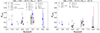 |
Fig. 9. Lyα fraction as a function of redshift. Blue, red, and green data points represent CEERS, JADES, and the combined sample. The open data points are obtained when we do not consider the galaxies in the overdensity at z ∼ 7.18 and z ∼ 7.49. Error bars are calculated from the binomial statistics described in Gehrels (1986). The black bar is the result obtained with the CodaII simulation at z = 7. Grey symbols are taken from literature, we provide the full list here in the same order as the legend: Stark et al. (2011), Tilvi et al. (2014), De Barros et al. (2017), Mason et al. (2018b, 2019), Pentericci et al. (2018a), Fuller et al. (2020), Kusakabe et al. (2020), Goovaerts et al. (2023), Jones et al. (2024), and Nakane et al. (2024). Some of the points have been slightly shifted in redshift for an easier visualization. |
Recently, also Nakane et al. (2024) and Jones et al. (2024) inferred Lyα visibilities during the EoR using JWST data. Jones et al. (2024) present the Lyα visibilities in the JADES sample (GOODS-South field) without applying a cut at the faint end of the MUV range. As expected, given that a large fraction of the JADES sources are fainter than MUV = −18.75, they obtain slightly higher Lyα visibilities than what we derived for the JADES sample, although fully consistent with our point. The recent analysis by Nakane et al. (2024) include data from JADES, GLASS, CEERS, and other programs, and also medium resolution gratings data are employed. Therefore, they analyzed a different set of data, with additional fields (as compared to our analysis). Applying our same cut both in MUV and EW0 > 25, they derived a value of  at z = 7 and a limit of < 0.19 at z > 8. Both results are in 1-σ agreement with what we derived.
In Fig. 9, we also report previous results from ground based observations from classical slit spectroscopy (Stark et al. 2011; Schenker et al. 2014; Tilvi et al. 2014; De Barros et al. 2017; Pentericci et al. 2018a; Fuller et al. 2020), MUSE integral field spectroscopy (Kusakabe et al. 2020; Goovaerts et al. 2023), and the KMOS spectrograph (Mason et al. 2019). In the case of Goovaerts et al. (2023) we examined the result obtained after completeness correction and when considering only continuum selected sources, which reproduces the LBG photometric selection more closely. Some of the above studies (e.g., Mason et al. 2019; Fuller et al. 2020; Goovaerts et al. 2023) target lensed galaxy fields, thereby probing intrinsically fainter galaxy population. In all the above studies we have selected fractions reported in the −20.25 < MUV < −18.75 range. The only exception is Goovaerts et al. (2023) that samples much fainter MUV (down to −12) and it is not immediately comparable. Our JWST Lyα fractions at z = 5 are lower than all previous results, although in some cases consistent within the errors. At z = 6 the comparison is harder as there is a wider range of published values: our combined value is consistent with some previous results but significantly lower than the values reported by Stark et al. (2011) and de Barros et al. (2016). At z = 7, the JADES fractions are consistent with previous estimates, while the CEERS fractions are larger, as already detailed above, even when removing the objects in the possible overdensities.
In Sect. 5.5 we further discuss why ground based and JWST observations might give substantially different Lyα results. If we take the JWST results alone at face value, the obtained average XLyα (from the combination of the CEERS and JADES observations) continues to rise from z = 5 to 7, dropping again at z = 8. This implies that either our results are not consistent with a rapid end of reionization that was inferred by previous works or that a rapid reionization ending is still characterized by > 1 pMpc bubbles around a high fraction of modestly bright galaxies, to at least z ∼ 7. Indeed, the large field-to-field variations imply a scenario in which multiple ionized bubbles can significantly alter the Lyα visibility, when considering only a limited area. This stresses the need for very large surveys in multiple fields, to obtain more robust results. In the following section, we further investigate this issue with the help of simulations.
5.2. Large field-to-field variations: Comparison to the CoDaII simulation
To further investigate if the large field to field variations are expected by the fundamental inhomogeneity of the reionization process, we employed calculations from the Cosmic Dawn II (CoDaII) simulation (Ocvirk et al. 2020). This simulation reproduces the reionization process to capture HII bubbles forming around star-forming galaxies on a grid of 40963 to resolve small-scale gas density and velocity structures, making it suitable for calculating Lyα opacity of the IGM (see Ocvirk et al. 2020 for more details). As described in Park et al. (2021), we calculate the Lyα visibility of simulated galaxies using CoDaII by integrating Lyα opacity along lines of sight. In particular, for each galaxy the transmission curve is obtained for ±4 Å around the rest-frame Lyα and for ∼2000 sight-lines, to account for the sight-line variation due to the stochasticity of HI density/velocity at small scales and the diversity of HII bubble shapes. We analyzed the Park et al. (2021) results at z = 7, using the same −20.25 < MUV < −18.75 cut to match the observations, and randomly selected 25 galaxies out of the simulated sample, to approximately match the number of target galaxies in the observations that are employed to calculate the z = 7 visibility in JADES and CEERS. We note that the simulated volume of the Universe at z = 7 is ∼760 000 cMpc3, that is twice the combined volume of the CEERS and JADES (GOODS-South) surveys. For each simulated galaxy, we randomly draw the intrinsic Lyα EW assuming an exponential declining distribution of the form P(EW)∝e−EW0/W0. We determine the free parameter W0 from the observed EW distribution of our sample at z < 6 (i.e., the post-reionization Universe) using both the Lyα-emitting sources and the limits on the non-emitting ones. We employed EMCEE (Foreman-Mackey et al. 2013) to conduct an MCMC fit and find W0 = (39 ± 2) Å. This result is in agreement with the value obtained in Pentericci et al. (2018a), when analyzing a very large sample of galaxies at z = 5.5 − 6.5 in the same MUV range.
The attenuation of Lyα EW is then calculated by taking the ratio between the integrated transmitted flux at the target redshift (z = 7 in this case) and the mean 55% transmission at the post-reionization redshift z = 6, which was calculated by Park et al. (2021). Finally we obtained the fraction of galaxies with EW0 > 25 (50) Å to simulate the visibility measurement from observations. We repeated this process 1000 times to obtain the average and standard deviation of the XLyα mock measurement sampling different lines of sight. We find that the fractions vary in the 2σ range [0.12, 0.48] ([0.02, 0.28]) for the 25 Å (50 Å) threshold. Such ranges are indeed similar to the observed difference between CEERS and JADES as shown in Fig. 9.
We focused our attention only on the large range of the simulated visibility and not on the central value, which is subject to both the reionization history of CoDaII and to the intrinsic emission model adopted in this calculation (i.e., the EW distribution in the post-reionization universe). As discussed above, this is still uncertain. Such a large uncertainty from the sight-line variation can be suppressed by enlarging the sample size in future surveys.
5.3. The ionized region in EGS at z = 7.18
As mentioned in Sect. 5.1, three of our LAEs are found within a very close redshift range (7.16−7.18). In particular one of the sources, ID 80374 has very high EW of (171 ± 41) Å. Since this source is very faint (MUV = −18.37), it is unlikely to have created a large ionized bubble to allow Lyα transmission by itself. For this reason Chen et al. (2024) argued that it might trace an overdensity. Indeed, the two other galaxies with Lyα emission (ID 439, and 498) are very close in sky coordinates, at a maximum (minimum) distance of 209″ (0.3″) from each other (Fig. 10). We also note that ID 829, which is listed in Table 1 as a tentative emitter is at the same redshift and also very close in sky coordinates. There are two more spectroscopically-confirmed sources from CEERS reported at a very similar redshift, ID 499 at z = 7.171 and ID 1038 at z = 7.196 (Mascia et al. 2024; Tang et al. 2023), which are not included in the present study since they were observed only in the medium-resolution grating NIRSpec configurations (G140M/F100LP, G235M/F170LP and G395M/F290LP). In particular, ID 499 is spatially very close at a distance of 0.28 pMpc from ID 498, although its spectrum does not show the Lyα emission line. We consider ID 499 to be part of the structure.
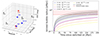 |
Fig. 10. Ionized bubble at z = 7.18. Left: position of the five spectroscopically-confirmed galaxies in the z ∼ 7.18 reionized region. Blue stars are the three LAEs with S/N > 3 and the red stars are the non-emitting ones, while we show the four photometric candidates with grey circles. Right: predicted size of an ionized bubble as a function of time since ionizing radiation is switched on. Solid coloured lines are for individual sources while the black solid line and shaded region represent the predicted size of the ionized bubble carved by the 5 galaxies together. The horizontal dashed line represents the physical bubble radius. |
In the following, we present a detailed analysis of the possible ionized bubble origin. We computed the size of the ionized bubble Rion that these five spectroscopically-confirmed galaxies could have carved through their ionizing photon capabilities to understand whether this could justify the enhanced Lyα visibility. We note that the separation between the most distant members along the line of sight (ID 80374 and ID 829) is 0.7 pMpc, while in the transverse direction, the maximum distance between the five sources is 1.1 pMpc (ID 80374 and ID 439). Therefore a rough estimate of the radius of the supposed ionized region is 0.62 pMpc, which we can consider to be the lower limit. The radius of the ionized bubble Rion that each of our sources could carve can be estimated following the approach detailed by Shapiro & Giroux (1987) and also used by other authors (e.g., Matthee et al. 2018; Larson et al. 2022; Saxena et al. 2023), taking into account its ionizing photon output Ṅion (in units of s−1), its ionizing escape fraction, and the time since it switched on:
 (2)
(2)
The quantity Ṅion, can be derived following Eq. (9) from Mason & Gronke (2020), that we report here:
 (3)
(3)
and depends on the MUV, the UV β slope, and the spectral slope of the ionizing continuum α which we assume is equal to unity, as found for galaxies at high z with massive stars (e.g., Steidel et al. 2014; Feltre et al. 2016). For the LyC escape fraction we employ the inferred quantities  derived in Sect. 4.3 for the emitters and the value reported in Table 1 of Mascia et al. (2024) for ID 499. In Fig. 10 (right panel) we present the derived bubble radius as a function of time elapsed since the sources have switched on which we let vary in the range 0−200 Myr. The results were obtained both individually for the five sources (three of which are LAEs) and for their combined output. The grey area represents the 1σ confidence region which takes into account the uncertainties in the MUV, β, and
  values, with the largest source of uncertainty being that on the
  .
.
Considering the joint ionizing output of the five confirmed sources, the size of the region that is ionized becomes compatible with the measured physical radius of the region for ages larger than ∼50 Myr, and with 1 pMpc for ages larger than ∼190 Myr. Therefore, the bubble could have been produced by these five sources if they have all switched on earlier than this time or if they have been “helped” by additional sources of ionizing radiation in the vicinity. Indeed, the photometric redshift catalog for the CEERS field (Finkelstein et al., in prep.) includes four more sources with photometric redshifts in the range [7.03−7.27] and in the same NIRSpec pointing (see Fig. 10). Three of them were placed in the MSA but no features or continuum are detected, possibly due to their faint magnitude (F115W ∼ 28.4), while the fourth one was not selected for the spectroscopic observations. Even if these four sources had relatively modest ionizing production and  as the five confirmed ones, their additional contribution would help create the large observed ionized bubble within even shorter timescales. We note that, at variance with early reionized regions discovered so far (e.g., Castellano et al. 2018; Matthee et al. 2018; Tilvi et al. 2020; Endsley & Stark 2022; Leonova et al. 2022), this bubble is not dominated by a UV bright source, whose large photon production might clear the path for the Lyα emission to become visible also from fainter nearby sources. In this case, all galaxies are relatively faint (−18 < MUV < −20) and also have modest inferred Lyman continuum escape fractions (0.02−0.23): it is only their combined output that creates a large enough ionized region.
5.4. The ionized regions in EGS at z = 7.49
Similarly, three LAEs (ID = 80432, 80372, and 80445 with S/N > 3) and a tentative emitter (ID = 80239 with S/N = 2) are found in the redshift range (7.48−7.51) within a maximum physical distance of 2.5 pMpc. Another galaxy (ID = 698) in the CEERS field, first identified by Roberts-Borsani et al. (2016), was confirmed to be at z = 7.473 from grating spectra (Mascia et al. 2024), but it is located several pMpc away from the four emitters. This structure was also noted by Chen et al. (2024) and it appears indeed much more extended than the one at z = 7.18. The brightest source in the structure is ID 80432 with a MUV = −20.22 and a high predicted escape fraction of  = 0.34. Following the same approach detailed before, we find that the ionizing photons coming from ID 80432 dominate over the contribution of the other three sources, which are all fainter and have very low inferred
  . The radius of the ionized region produced by the four spectroscopically-confirmed galaxies considered becomes compatible to the physical radius of the observed region (∼1.2 pMpc) for ages larger than 200 Myr. Since it is unlikely that star formation is sustained in all sources over such a long timescale (e.g., Cole et al. 2023), a better explanation could be that we have missed sources that are contributing to the formation of the ionizing the bubble. Therefore, we also checked the CEERS photometric redshift catalog (Finkelstein et al., in prep.) to search for possible additional photometric candidates in the region: although there are several sources with photometric redshift compatible with z ∼ 7.5, they are spatially offset from the confirmed emitters. It is therefore unclear if the sources reside in a unique very large ionized region (∼2−3 pMpc), or alternatively if they are in separate smaller bubbles (< 1 pMpc). Only high-resolution spectroscopy could shed light on this point, by providing the missing information on the Lyα velocity offset: if small offsets are observed, then the line emission is consistent with a single large ionized bubble (e.g., see Fig. 1 from Mason & Gronke 2020).
5.5. Comparison with ground based observations
The Lyα visibilities we have derived in Sect. 5 are somewhat at odds with previous ground based derivations. In particular, our fractions are lower than most previous determinations at ∼5 and 6 and higher at z ∼ 7. We first remark that prior to the advent of JWST most samples were identified on the basis of photometric redshifts whenever Lyα was not present; however, in this study, all the galaxies used to compute Lyα visibility are spectroscopically-confirmed, thanks to the identification of optical lines in the spectra. This, together with the lack of telluric lines from space improves dramatically our ability to identify Lyα even at low S/N and to probe secure limits when the line is not detected.
Also, as noted in Sect. 5.1, the discrepancy is clearly driven by the field-to-field variations and by the inhomogeneity of the IGM conditions and the possible presence of peculiar ionized regions in some fields. However, the discrepancy might also be due to the different Lyα flux that is measured in NIRSpec MSA spectra compared to ground based slit spectroscopy. The different EW values recovered have already been noted for several individual objects that boast both JWST and ground based slit spectroscopy observations (including some of the CEERS galaxies e.g., by Larson et al. 2023b; Jiang et al. 2023; Tang et al. 2023, 2024; Chen et al. 2024). In most cases the derived Lyα fluxes are smaller when measured from the NIRSpec MSA observations. Recently, Nakane et al. (2024) estimated that the EW values recovered by JWST NIRSpec are ≃70% of the values measured by ground-based instruments such as FORS2 (see Fig. B.3 in their paper). Jiang et al. (2023) also discussed the non detection by deep JWST NIRSpec PRISM spectroscopy of a previously known LAE in the A2744 field at z = 5.66.
The MSA pseudo slits are indeed much smaller than the slits employed in ground-based programs, which are typically matched to the seeing, and vary from 0.7″ to 1.0″ (Schenker et al. 2012; Pentericci et al. 2014). The MSA might therefore miss part of the Lyα flux due to various effects including (i) the presence of spatial offsets between the UV and Lyα emission, with MSA typically placed on the rest-frame UV emission barycenter; (ii) a spatially extended diffuse Lyα emission, due to resonant scattering of the Lyα photons on the neutral hydrogen inside the galaxies; and (iii) differential dust extinction and inhomogeneous neutral ISM structure within the galaxies.
Hoag et al. (2019) presented the first systematic study of Lyα vs UV offsets finding that they are generally small, on the order of 0.2″ at z ∼ 5 (corresponding to 1.3 kpc) and decrease towards high redshifts. This trend is also consistent with the most recent results obtained by Ning et al. (2024) on a small sample of bright Lyα-emitting sources in the COSMOS-Web survey also observed with NIRCam, for which they find a median offset of 0.12″ at z ∼ 6, and by Lemaux et al. (2021), who studied a large sample of emitters, including lensed sources and found an average offset of 0.11″ at 5 < z < 7. Therefore, the predicted offset at z = 7 would be smaller than the MSA size but comparable to the MSA size at lower redshift. This could imply that the discrepancy between the ground based results and JWST ones is more significant at z < 6 than at higher redshift, which could partially explain our lower Lyα fractions at z = 5 and 6.
Even in the absence of significant offset, the Lyα emission could be more spatially extended than the UV emission, due to the fact that Lyα photons are resonantly scattered by the neutral hydrogen atoms inside the galaxies. This was first shown by narrow band imaging capturing the Lyα emission (Steidel et al. 2011) and, more recently, by MUSE observations (Leclercq et al. 2017; Kusakabe et al. 2022) indicating that a large fraction (around 80%) of high redshift star forming galaxies show diffuse Lyα halos, whose scale length is up to 10 times larger than the UV emission (although with a very large scatter). Such halos seem to be more important for very bright objects (see also Matthee et al. 2020). The contribution of the halo to the total Lyα flux is at least a factor of 2, and this quantity does not seem to be related to other galaxy properties. The median scale length of the halos of ∼4−5 kpc (Leclercq et al. 2017) means that the large slits employed in ground based observations and the IFUs, can still recover most of the flux, while the same would not be true for the much smaller MSA pseudoslits. Again, this could be a redshift dependent effect, with the discrepancy becoming less evident at high redshift when galaxies become more compact. Finally, dust produced in the star forming events suppress the Lyα emission and, depending on its spatial distribution, it could differentially attenuate some regions more than others. Additionally, the uneven structure of the neutral ISM within the galaxy, as highlighted by Hu et al. (2023) for local galaxies, influences Lyα visibility. These combined effects also contribute to produce the mismatch between ground-based and space observations.
As demonstrated by Maiolino et al. (2024) for the AGN GN-z11, NIRSpec-IFU observations in the future could help us to interpret this mismatch and reconcile space and ground based Lyα observations. By capturing flux from larger regions, we would be able to investigate the spatial extent of Lyα emission – as was previously done for low-z Lyα emitters from ground based MUSE observations. This would allow us to understand how it impacts the derivation of the Lyα visibility evolution.
6. Summary
We have presented the results of a comprehensive study of the evolution of Lyα emission from galaxies at 4.5 < z < 8.5. The CEERS sample consists of 144 galaxies in the EGS field at 4.1 < z < 9.8, each with secure spectroscopic redshifts identified through multiple optical line detection. We identified 43 secure (S/N > 3) Lyα emitting galaxies and 7 tentative ones (2 < S/N < 3), while 94 galaxies have no Lyα emission. We supplemented the CEERS dataset with 91 additional galaxies with published data from the JADES GOODS-South survey, of which 15 have Lyα in emission. Therefore, in this study we considered 235 galaxies (at 4.1 < z < 9.9) with homogeneous JWST NIRSpec PRISM/CLEAR data selected through photometric redshifts, of which in total 65 show Lyα in emission. We summarize our main results in the following:
-
We computed the Lyα escape fractions (
 ) and explored the correlations between
  and the physical properties of the galaxies. We measured low values of
  in dusty, massive, UV bright galaxies. These sources probably have larger amounts of hydrogen and dust in their ISM and, due to the resonant scattering of Lyα photons, these characteristics attenuate the emission we observe. We find only a marginal (p-value = 3 × 10⁻²) anticorrelation with the half-light radius. The correlations do not vary much with redshift.
 -
We predicted the escape fraction of LyC photons (
 ) using two empirical relations, based on well-explored indirect indicators derived at z ∼ 0.3. Contrary to the expectation from lower redshift results and from theoretical models of LyC escape, we did not find any solid correlations (p-value > 0.1) between
  and
and  either in the ionized universe (z < 5.5) or during the epoch of reionization, although the sample considered is rather small and the uncertainties on the LyC escape fractions are still significant.
 -
We determined the redshift evolution of the Lyα visibility (XLyα), namely, the fraction of galaxies with a Lyα rest frame equivalent width EW0 > 25 Å (and > 50 Å) in four redshift bins at 4.5 < z < 8.5, for the CEERS and the JADES subsets separately and as a whole. We found significantly lower Lyα fractions at z = 5 and 6 compared to previous ground-based observations. At z = 7, while the JADES fraction is consistent with previous results, the visibility in the CEERS field appears much enhanced, probably due to two ionized regions at z = 7.18 and z = 7.49. We highlight that the average XLyα derived from the combined CEERS+JADES data continues to rise from z = 5 to 7, dropping again at z = 8. This implies that either our results are not consistent with a rapid end of reionization, or that a rapid reionization ending is still characterized by > 1 pMpc bubbles around a high fraction of modestly bright galaxies, to at least z ∼ 7.
-
We further investigate the effect of cosmic variance whose substantial effect on the observational data is suggested by the large difference of XLyα between CEERS and JADES. We employed the Cosmic Dawn II (CoDaII) simulation to calculate the predicted Lyα visibility at z = 7 in a ∼760 000 cMpc3 volume. The uncertainty range of the mock measurement is similar to the difference between the two fields and stresses the paramount importance of acquiring more data on a larger number of independent fields, to obtain a more robust redshift evolution of the Lyα emitter fraction.
-
We further characterized the two ionized regions in the EGS at z = 7.18 and z = 7.49, which both have three secure (S/N > 3) and one tentative (S/N ∼ 2) LAEs. We computed the radius of the ionized bubble Rion that each of the spectroscopically-confirmed members of the ionized region could carve either individually or as an ensemble. For the z = 7.18 bubble, the observed physical radius Rion ∼ 0.6 pMpc can be achieved by sustained star-formation activity over ∼50 Myr or less if helped by additional ionizing sources. For the z = 7.49 bubble, the observed radius of ∼1.2 pMpc could only be achieved for ages larger than ∼200 Myr. Although, it is unlikely that sources could sustain star formation over such a long timescale, making the nature of this region enigmatic.
-
In this work, we discuss the possible effects that can impact the Lyα emission measurement through the NIRSpec MSA pseudo slits, and how they can differ from the ground-based slit measurements. The well studied presence of spatial offsets between the Lyα and UV emission, the spatially diffuse nature of Lyα emission, and differential dust extinction all bring on substantial effects, which might change with redshift. Consequently, it is not possible to study the evolution of the Lyα visibility combining low-redshift results from ground based telescopes with z ≥ 7 measurements from JWST.
Essential insights could emerge from future NIRSpec-IFU observations, aiding in harmonizing space and ground-based Lyα observations. The potential to capture flux from larger regions opens avenues to explore the spatial extent of Lyα emission, akin to previous studies on low-z Lyα emitters using ground-based MUSE observations, offering valuable insights into how it impacts the derivation of the Lyα visibility evolution. Future larger surveys covering additional fields will be needed to reduce the chances of the samples being biased to overdense or underdense regions (as in the present study), overcome cosmic variance, and provide a number of sources large enough to compute the spatial variation of χHI with a high statistical significance.
Acknowledgments
We thank the anonymous referee for the constructive feedback provided. We acknowledge support from the PRIN 2022 MUR project 2022CB3PJ3 – First Light And Galaxy aSsembly (FLAGS) funded by the European Union – Next Generation EU. L.N. thanks Arianna Favale for providing valuable insights into the MCMC fitting procedure.
References
- Adams, N. J., Conselice, C. J., Ferreira, L., et al. 2023, MNRAS, 518, 4755 [Google Scholar]
- Arrabal Haro, P., Rodríguez Espinosa, J. M., Muñoz-Tuñón, C., et al. 2018, MNRAS, 478, 3740 [NASA ADS] [CrossRef] [Google Scholar]
- Arrabal Haro, P., Dickinson, M., Finkelstein, S. L., et al. 2023a, ApJ, 951, L22 [NASA ADS] [CrossRef] [Google Scholar]
- Arrabal Haro, P., Dickinson, M., Finkelstein, S. L., et al. 2023b, Nature, 622, 707 [NASA ADS] [CrossRef] [Google Scholar]
- Atek, H., Shuntov, M., Furtak, L. J., et al. 2023, MNRAS, 519, 1201 [Google Scholar]
- Bañados, E., Venemans, B. P., Mazzucchelli, C., et al. 2018, Nature, 553, 473 [Google Scholar]
- Bagley, M. B., Finkelstein, S. L., Koekemoer, A. M., et al. 2023, ApJ, 946, L12 [NASA ADS] [CrossRef] [Google Scholar]
- Bagley, M. B., Pirzkal, N., Finkelstein, S. L., et al. 2024, ApJ, 965, L6 [NASA ADS] [CrossRef] [Google Scholar]
- Becker, G. D., Bolton, J. S., & Lidz, A. 2015a, PASA, 32, e045 [NASA ADS] [CrossRef] [Google Scholar]
- Becker, G. D., Bolton, J. S., Madau, P., et al. 2015b, MNRAS, 447, 3402 [Google Scholar]
- Becker, G. D., D’Aloisio, A., Christenson, H. M., et al. 2021, MNRAS, 508, 1853 [NASA ADS] [CrossRef] [Google Scholar]
- Begley, R., Cullen, F., McLure, R. J., et al. 2024, MNRAS, 527, 4040 [Google Scholar]
- Bhatawdekar, R., Conselice, C. J., Margalef-Bentabol, B., & Duncan, K. 2019, MNRAS, 486, 3805 [NASA ADS] [CrossRef] [Google Scholar]
- Bosman, S. E. I., Davies, F. B., Becker, G. D., et al. 2022, MNRAS, 514, 55 [NASA ADS] [CrossRef] [Google Scholar]
- Bouwens, R. J., Illingworth, G. D., Oesch, P. A., et al. 2015, ApJ, 811, 140 [NASA ADS] [CrossRef] [Google Scholar]
- Bouwens, R. J., Stefanon, M., Brammer, G., et al. 2023, MNRAS, 523, 1036 [NASA ADS] [CrossRef] [Google Scholar]
- Brammer, G. B., van Dokkum, P. G., & Coppi, P. 2008, ApJ, 686, 1503 [Google Scholar]
- Bruzual, G., & Charlot, S. 2003, MNRAS, 344, 1000 [NASA ADS] [CrossRef] [Google Scholar]
- Bunker, A. J., NIRSPEC Instrument Science Team,& JAESs Collaboration 2020, in Uncovering Early Galaxy Evolution in the ALMA and JWST Era, eds. E. da Cunha, J. Hodge, J. Afonso, L. Pentericci, & D. Sobral, 352, 342 [NASA ADS] [Google Scholar]
- Bunker, A. J., Saxena, A., Cameron, A. J., et al. 2023a, A&A, 677, A88 [NASA ADS] [CrossRef] [EDP Sciences] [Google Scholar]
- Bunker, A. J., Cameron, A. J., Curtis-Lake, E., et al. 2023b, A&A, submitted [arXiv:2306.02467] [Google Scholar]
- Calabrò, A., Castellano, M., Pentericci, L., et al. 2021, A&A, 646, A39 [EDP Sciences] [Google Scholar]
- Calzetti, D., Kinney, A. L., & Storchi-Bergmann, T. 1994, ApJ, 429, 582 [Google Scholar]
- Calzetti, D., Armus, L., Bohlin, R. C., et al. 2000, ApJ, 533, 682 [NASA ADS] [CrossRef] [Google Scholar]
- Caruana, J., Bunker, A. J., Wilkins, S. M., et al. 2014, MNRAS, 443, 2831 [NASA ADS] [CrossRef] [Google Scholar]
- Caruana, J., Wisotzki, L., Herenz, E. C., et al. 2018, MNRAS, 473, 30 [NASA ADS] [CrossRef] [Google Scholar]
- Casey, C. M., Akins, H. B., Shuntov, M., et al. 2024, ApJ, 965, 98 [NASA ADS] [CrossRef] [Google Scholar]
- Castellano, M., Sommariva, V., Fontana, A., et al. 2014, A&A, 566, A19 [NASA ADS] [CrossRef] [EDP Sciences] [Google Scholar]
- Castellano, M., Dayal, P., Pentericci, L., et al. 2016, ApJ, 818, L3 [NASA ADS] [CrossRef] [Google Scholar]
- Castellano, M., Pentericci, L., Vanzella, E., et al. 2018, ApJ, 863, L3 [CrossRef] [Google Scholar]
- Castellano, M., Fontana, A., Treu, T., et al. 2022, ApJ, 938, L15 [NASA ADS] [CrossRef] [Google Scholar]
- Chabrier, G. 2003, PASP, 115, 763 [Google Scholar]
- Chen, Z., Stark, D. P., Mason, C., et al. 2024, MNRAS, 528, 7052 [CrossRef] [Google Scholar]
- Chisholm, J., Saldana-Lopez, A., Flury, S., et al. 2022, MNRAS, 517, 5104 [CrossRef] [Google Scholar]
- Choustikov, N., Katz, H., Saxena, A., et al. 2024, MNRAS, 529, 3751 [NASA ADS] [CrossRef] [Google Scholar]
- Cole, J. W., Papovich, C., Finkelstein, S. L., et al. 2023, arXiv e-prints [arXiv:2312.10152] [Google Scholar]
- Davis, M., Guhathakurta, P., Konidaris, N. P., et al. 2007, ApJ, 660, L1 [NASA ADS] [CrossRef] [Google Scholar]
- Davis, K., Trump, J. R., Simons, R. C., et al. 2023, ApJ, submitted [arXiv:2312.07799] [Google Scholar]
- Dawoodbhoy, T., Shapiro, P. R., Ocvirk, P., et al. 2018, MNRAS, 480, 1740 [CrossRef] [Google Scholar]
- de Barros, S., Vanzella, E., Amorín, R., et al. 2016, A&A, 585, A51 [NASA ADS] [CrossRef] [EDP Sciences] [Google Scholar]
- De Barros, S., Pentericci, L., Vanzella, E., et al. 2017, A&A, 608, A123 [NASA ADS] [CrossRef] [EDP Sciences] [Google Scholar]
- Developers, J., Averbukh, J., Bradley, L., et al. 2023, https://doi.org/10.5281/zenodo.7504710 [Google Scholar]
- Dijkstra, M. 2017, arXiv e-prints [arXiv:1704.03416] [Google Scholar]
- Dijkstra, M., Gronke, M., & Venkatesan, A. 2016, ApJ, 828, 71 [Google Scholar]
- Ding, X., Silverman, J., Treu, T., et al. 2020, ApJ, 888, 37 [NASA ADS] [CrossRef] [Google Scholar]
- Eisenstein, D. J., Willott, C., Alberts, S., et al. 2023, ApJS, submitted [arXiv:2306.02465] [Google Scholar]
- Endsley, R., & Stark, D. P. 2022, MNRAS, 511, 6042 [NASA ADS] [CrossRef] [Google Scholar]
- Fan, X., Strauss, M. A., Becker, R. H., et al. 2006, AJ, 132, 117 [NASA ADS] [CrossRef] [Google Scholar]
- Feltre, A., Charlot, S., & Gutkin, J. 2016, MNRAS, 456, 3354 [Google Scholar]
- Finkelstein, S. L., Ryan, R. E., Papovich, C., et al. 2015, ApJ, 810, 71 [NASA ADS] [CrossRef] [Google Scholar]
- Finkelstein, S. L., D’Aloisio, A., Paardekooper, J.-P., et al. 2019, ApJ, 879, 36 [Google Scholar]
- Finkelstein, S. L., Bagley, M. B., Haro, P. A., et al. 2022a, ApJ, 940, L55 [NASA ADS] [CrossRef] [Google Scholar]
- Finkelstein, S. L., Bagley, M., Song, M., et al. 2022b, ApJ, 928, 52 [CrossRef] [Google Scholar]
- Finkelstein, S. L., Bagley, M. B., Ferguson, H. C., et al. 2023, ApJ, 946, L13 [NASA ADS] [CrossRef] [Google Scholar]
- Flury, S. R., Jaskot, A. E., Ferguson, H. C., et al. 2022, ApJS, 260, 1 [NASA ADS] [CrossRef] [Google Scholar]
- Fontana, A., D’Odorico, S., Poli, F., et al. 2000, AJ, 120, 2206 [NASA ADS] [CrossRef] [Google Scholar]
- Fontana, A., Vanzella, E., Pentericci, L., et al. 2010, ApJ, 725, L205 [Google Scholar]
- Foreman-Mackey, D., Hogg, D. W., Lang, D., & Goodman, J. 2013, PASP, 125, 306 [Google Scholar]
- Fuller, S., Lemaux, B. C., Bradač, M., et al. 2020, ApJ, 896, 156 [NASA ADS] [CrossRef] [Google Scholar]
- Gaikwad, P., Rauch, M., Haehnelt, M. G., et al. 2020, MNRAS, 494, 5091 [Google Scholar]
- Gardner, J. P., Mather, J. C., Clampin, M., et al. 2006, Space Sci. Rev., 123, 485 [Google Scholar]
- Gardner, J. P., Mather, J. C., Abbott, R., et al. 2023, PASP, 135, 068001 [NASA ADS] [CrossRef] [Google Scholar]
- Gazagnes, S., Chisholm, J., Schaerer, D., Verhamme, A., & Izotov, Y. 2020, A&A, 639, A85 [NASA ADS] [CrossRef] [EDP Sciences] [Google Scholar]
- Gehrels, N. 1986, ApJ, 303, 336 [Google Scholar]
- Giallongo, E., Grazian, A., Fiore, F., et al. 2015, A&A, 578, A83 [NASA ADS] [CrossRef] [EDP Sciences] [Google Scholar]
- Giavalisco, M., Ferguson, H. C., Koekemoer, A. M., et al. 2004, ApJ, 600, L93 [NASA ADS] [CrossRef] [Google Scholar]
- Goovaerts, I., Pello, R., Thai, T. T., et al. 2023, A&A, 678, A174 [NASA ADS] [CrossRef] [EDP Sciences] [Google Scholar]
- Grogin, N. A., Kocevski, D. D., Faber, S. M., et al. 2011, ApJS, 197, 35 [NASA ADS] [CrossRef] [Google Scholar]
- Gurung-López, S., Gronke, M., Saito, S., Bonoli, S., & Orsi, Á. A. 2022, MNRAS, 510, 4525 [NASA ADS] [CrossRef] [Google Scholar]
- Harikane, Y., Ouchi, M., Ono, Y., et al. 2019, ApJ, 883, 142 [Google Scholar]
- Harikane, Y., Ouchi, M., Oguri, M., et al. 2023a, ApJS, 265, 5 [NASA ADS] [CrossRef] [Google Scholar]
- Harikane, Y., Zhang, Y., Nakajima, K., et al. 2023b, ApJ, 959, 39 [NASA ADS] [CrossRef] [Google Scholar]
- Hassan, S., Davé, R., Mitra, S., et al. 2018, MNRAS, 473, 227 [Google Scholar]
- Hayes, M., Schaerer, D., Östlin, G., et al. 2011, ApJ, 730, 8 [NASA ADS] [CrossRef] [Google Scholar]
- Hayes, M., Östlin, G., Duval, F., et al. 2014, ApJ, 782, 6 [NASA ADS] [CrossRef] [Google Scholar]
- Hoag, A., Treu, T., Pentericci, L., et al. 2019, MNRAS, 488, 706 [Google Scholar]
- Holwerda, B. W., Bouwens, R., Oesch, P., et al. 2015, ApJ, 808, 6 [CrossRef] [Google Scholar]
- Hu, E. M., & McMahon, R. G. 1996, Nature, 382, 231 [Google Scholar]
- Hu, W., Wang, J., Zheng, Z.-Y., et al. 2019, ApJ, 886, 90 [NASA ADS] [CrossRef] [Google Scholar]
- Hu, W., Martin, C. L., Gronke, M., et al. 2023, ApJ, 956, 39 [CrossRef] [Google Scholar]
- Inoue, A. K., Shimizu, I., Iwata, I., & Tanaka, M. 2014, MNRAS, 442, 1805 [NASA ADS] [CrossRef] [Google Scholar]
- Itoh, R., Ouchi, M., Zhang, H., et al. 2018, ApJ, 867, 46 [NASA ADS] [CrossRef] [Google Scholar]
- Jakobsen, P., Ferruit, P., Alves de Oliveira, C., et al. 2022, A&A, 661, A80 [NASA ADS] [CrossRef] [EDP Sciences] [Google Scholar]
- Jaskot, A. E., Dowd, T., Oey, M. S., Scarlata, C., & McKinney, J. 2019, ApJ, 885, 96 [Google Scholar]
- Jiang, L., Ning, Y., Fan, X., et al. 2022, Nat. Astron., 6, 850 [NASA ADS] [CrossRef] [Google Scholar]
- Jiang, H., Wang, X., Cheng, C., et al. 2023, arXiv e-prints [arXiv:2312.04151] [Google Scholar]
- Jones, G. C., Bunker, A. J., Saxena, A., et al. 2024, A&A, 683, A238 [NASA ADS] [CrossRef] [EDP Sciences] [Google Scholar]
- Jung, I., Finkelstein, S. L., Dickinson, M., et al. 2019, ApJ, 877, 146 [CrossRef] [Google Scholar]
- Jung, I., Finkelstein, S. L., Dickinson, M., et al. 2020, ApJ, 904, 144 [NASA ADS] [CrossRef] [Google Scholar]
- Jung, I., Finkelstein, S. L., Larson, R. L., et al. 2022, arXiv e-prints [arXiv:2212.09850] [Google Scholar]
- Jung, I., Finkelstein, S. L., Arrabal Haro, P., et al. 2024, ApJ, 967, 73 [NASA ADS] [CrossRef] [Google Scholar]
- Kocevski, D. D., Onoue, M., Inayoshi, K., et al. 2023, ApJ, 954, L4 [NASA ADS] [CrossRef] [Google Scholar]
- Koekemoer, A. M., Faber, S. M., Ferguson, H. C., et al. 2011, ApJS, 197, 36 [NASA ADS] [CrossRef] [Google Scholar]
- Konno, A., Ouchi, M., Shibuya, T., et al. 2018, PASJ, 70, S16 [Google Scholar]
- Kulkarni, G., Worseck, G., & Hennawi, J. F. 2019, MNRAS, 488, 1035 [Google Scholar]
- Kusakabe, H., Blaizot, J., Garel, T., et al. 2020, A&A, 638, A12 [NASA ADS] [CrossRef] [EDP Sciences] [Google Scholar]
- Kusakabe, H., Verhamme, A., Blaizot, J., et al. 2022, A&A, 660, A44 [NASA ADS] [CrossRef] [EDP Sciences] [Google Scholar]
- Larson, R. L., Finkelstein, S. L., Pirzkal, N., et al. 2018, ApJ, 858, 94 [NASA ADS] [CrossRef] [Google Scholar]
- Larson, R. L., Finkelstein, S. L., Hutchison, T. A., et al. 2022, ApJ, 930, 104 [NASA ADS] [CrossRef] [Google Scholar]
- Larson, R. L., Hutchison, T. A., Bagley, M., et al. 2023a, ApJ, 958, 141 [NASA ADS] [CrossRef] [Google Scholar]
- Larson, R. L., Finkelstein, S. L., Kocevski, D. D., et al. 2023b, ApJ, 953, L29 [NASA ADS] [CrossRef] [Google Scholar]
- Leclercq, F., Bacon, R., Wisotzki, L., et al. 2017, A&A, 608, A8 [NASA ADS] [CrossRef] [EDP Sciences] [Google Scholar]
- Lemaux, B. C., Fuller, S., Bradač, M., et al. 2021, MNRAS, 504, 3662 [NASA ADS] [CrossRef] [Google Scholar]
- Leonova, E., Oesch, P. A., Qin, Y., et al. 2022, MNRAS, 515, 5790 [NASA ADS] [CrossRef] [Google Scholar]
- Lin, X., Cai, Z., Wu, Y., et al. 2024, ApJS, 272, 33 [NASA ADS] [CrossRef] [Google Scholar]
- Livermore, R. C., Finkelstein, S. L., & Lotz, J. M. 2017, ApJ, 835, 113 [Google Scholar]
- Luo, B., Brandt, W. N., Xue, Y. Q., et al. 2017, ApJS, 228, 2 [Google Scholar]
- Maiolino, R., Scholtz, J., Curtis-Lake, E., et al. 2023, A&A, submitted [arXiv:2308.01230] [Google Scholar]
- Maiolino, R., Übler, H., Perna, M., et al. 2024, A&A, 687, A67 [NASA ADS] [CrossRef] [EDP Sciences] [Google Scholar]
- Marchi, F., Pentericci, L., Guaita, L., et al. 2017, A&A, 601, A73 [NASA ADS] [CrossRef] [EDP Sciences] [Google Scholar]
- Marchi, F., Pentericci, L., Guaita, L., et al. 2019, A&A, 631, A19 [NASA ADS] [CrossRef] [EDP Sciences] [Google Scholar]
- Markwardt, C. B. 2009, ASP Conf. Ser., 411, 251 [Google Scholar]
- Mascia, S., Pentericci, L., Calabrò, A., et al. 2023, A&A, 672, A155 [NASA ADS] [CrossRef] [EDP Sciences] [Google Scholar]
- Mascia, S., Pentericci, L., Calabrò, A., et al. 2024, A&A, 685, A3 [NASA ADS] [CrossRef] [EDP Sciences] [Google Scholar]
- Mason, C. A., & Gronke, M. 2020, MNRAS, 499, 1395 [Google Scholar]
- Mason, C. A., Treu, T., de Barros, S., et al. 2018a, ApJ, 857, L11 [Google Scholar]
- Mason, C. A., Treu, T., Dijkstra, M., et al. 2018b, ApJ, 856, 2 [Google Scholar]
- Mason, C. A., Fontana, A., Treu, T., et al. 2019, MNRAS, 485, 3947 [NASA ADS] [CrossRef] [Google Scholar]
- Matsuoka, Y., Strauss, M. A., Kashikawa, N., et al. 2018, ApJ, 869, 150 [Google Scholar]
- Matthee, J., Sobral, D., Gronke, M., et al. 2018, A&A, 619, A136 [NASA ADS] [CrossRef] [EDP Sciences] [Google Scholar]
- Matthee, J., Pezzulli, G., Mackenzie, R., et al. 2020, MNRAS, 498, 3043 [Google Scholar]
- Matthee, J., Naidu, R. P., Brammer, G., et al. 2024, ApJ, 963, 129 [NASA ADS] [CrossRef] [Google Scholar]
- Merlin, E., Bonchi, A., Paris, D., et al. 2022, ApJ, 938, L14 [NASA ADS] [CrossRef] [Google Scholar]
- Meurer, G. R., Heckman, T. M., & Calzetti, D. 1999, ApJ, 521, 64 [Google Scholar]
- Morishita, T., Trenti, M., Stiavelli, M., et al. 2018, ApJ, 867, 150 [NASA ADS] [CrossRef] [Google Scholar]
- Naidu, R. P., Oesch, P. A., van Dokkum, P., et al. 2022, ApJ, 940, L14 [NASA ADS] [CrossRef] [Google Scholar]
- Nakajima, K., Ouchi, M., Isobe, Y., et al. 2023, ApJS, 269, 33 [NASA ADS] [CrossRef] [Google Scholar]
- Nakane, M., Ouchi, M., Nakajima, K., et al. 2024, ApJ, 967, 28 [NASA ADS] [CrossRef] [Google Scholar]
- Nandra, K., Laird, E. S., Aird, J. A., et al. 2015, ApJS, 220, 10 [NASA ADS] [CrossRef] [Google Scholar]
- Napolitano, L., Pentericci, L., Calabrò, A., et al. 2023, A&A, 677, A138 [NASA ADS] [CrossRef] [EDP Sciences] [Google Scholar]
- Ning, Y., Cai, Z., Lin, X., et al. 2024, ApJ, 963, L38 [NASA ADS] [CrossRef] [Google Scholar]
- Ocvirk, P., Aubert, D., Sorce, J. G., et al. 2020, MNRAS, 496, 4087 [NASA ADS] [CrossRef] [Google Scholar]
- Ocvirk, P., Lewis, J. S. W., Gillet, N., et al. 2021, MNRAS, 507, 6108 [NASA ADS] [CrossRef] [Google Scholar]
- Oke, J. B., & Gunn, J. E. 1983, ApJ, 266, 713 [NASA ADS] [CrossRef] [Google Scholar]
- Ono, Y., Ouchi, M., Mobasher, B., et al. 2012, ApJ, 744, 83 [Google Scholar]
- Osterbrock, D. E., & Ferland, G. J. 2006, Astrophysics of Gaseous Nebulae and Active Galactic Nuclei (Sausalito: University Science Books) [Google Scholar]
- Ota, K., Iye, M., Kashikawa, N., et al. 2008, ApJ, 677, 12 [NASA ADS] [CrossRef] [Google Scholar]
- Ouchi, M., Shimasaku, K., Furusawa, H., et al. 2010, ApJ, 723, 869 [Google Scholar]
- Ouchi, M., Ono, Y., & Shibuya, T. 2020, ARA&A, 58, 617 [Google Scholar]
- Pahl, A. J., Shapley, A., Steidel, C. C., Chen, Y., & Reddy, N. A. 2021, MNRAS, 505, 2447 [NASA ADS] [CrossRef] [Google Scholar]
- Park, H., Jung, I., Song, H., et al. 2021, ApJ, 922, 263 [NASA ADS] [CrossRef] [Google Scholar]
- Parsa, S., Dunlop, J. S., & McLure, R. J. 2018, MNRAS, 474, 2904 [Google Scholar]
- Pentericci, L., Fontana, A., Vanzella, E., et al. 2011, ApJ, 743, 132 [NASA ADS] [CrossRef] [Google Scholar]
- Pentericci, L., Vanzella, E., Fontana, A., et al. 2014, ApJ, 793, 113 [NASA ADS] [CrossRef] [Google Scholar]
- Pentericci, L., Vanzella, E., Castellano, M., et al. 2018a, A&A, 619, A147 [NASA ADS] [CrossRef] [EDP Sciences] [Google Scholar]
- Pentericci, L., McLure, R. J., Garilli, B., et al. 2018b, A&A, 616, A174 [NASA ADS] [CrossRef] [EDP Sciences] [Google Scholar]
- Planck Collaboration VI. 2020, A&A, 641, A6 [NASA ADS] [CrossRef] [EDP Sciences] [Google Scholar]
- Rieke, M. J., Robertson, B., Tacchella, S., et al. 2023, ApJS, 269, 16 [NASA ADS] [CrossRef] [Google Scholar]
- Roberts-Borsani, G. W., Bouwens, R. J., Oesch, P. A., et al. 2016, ApJ, 823, 143 [NASA ADS] [CrossRef] [Google Scholar]
- Robertson, B. E., Furlanetto, S. R., Schneider, E., et al. 2013, ApJ, 768, 71 [Google Scholar]
- Roy, N., Henry, A., Treu, T., et al. 2023, ApJ, 952, L14 [NASA ADS] [CrossRef] [Google Scholar]
- Sandles, L., D’Eugenio, F., Maiolino, R., et al. 2023, arXiv e-prints [arXiv:2306.03931] [Google Scholar]
- Santini, P., Castellano, M., Fontana, A., et al. 2022, ApJ, 940, 135 [NASA ADS] [CrossRef] [Google Scholar]
- Saxena, A., Robertson, B. E., Bunker, A. J., et al. 2023, A&A, 678, A68 [NASA ADS] [CrossRef] [EDP Sciences] [Google Scholar]
- Saxena, A., Bunker, A. J., Jones, G. C., et al. 2024, A&A, 684, A84 [NASA ADS] [CrossRef] [EDP Sciences] [Google Scholar]
- Schaerer, D., & de Barros, S. 2009, A&A, 502, 423 [NASA ADS] [CrossRef] [EDP Sciences] [Google Scholar]
- Schenker, M. A., Stark, D. P., Ellis, R. S., et al. 2012, ApJ, 744, 179 [Google Scholar]
- Schenker, M. A., Ellis, R. S., Konidaris, N. P., & Stark, D. P. 2014, ApJ, 795, 20 [NASA ADS] [CrossRef] [Google Scholar]
- Shapiro, P. R., & Giroux, M. L. 1987, ApJ, 321, L107 [NASA ADS] [CrossRef] [Google Scholar]
- Song, M., Finkelstein, S. L., Livermore, R. C., et al. 2016, ApJ, 826, 113 [NASA ADS] [CrossRef] [Google Scholar]
- Stark, D. P., Ellis, R. S., Chiu, K., Ouchi, M., & Bunker, A. 2010, MNRAS, 408, 1628 [Google Scholar]
- Stark, D. P., Ellis, R. S., & Ouchi, M. 2011, ApJ, 728, L2 [Google Scholar]
- Stefanon, M., Yan, H., Mobasher, B., et al. 2017, ApJS, 229, 32 [NASA ADS] [CrossRef] [Google Scholar]
- Steidel, C. C., Giavalisco, M., Pettini, M., Dickinson, M., & Adelberger, K. L. 1996, ApJ, 462, L17 [Google Scholar]
- Steidel, C. C., Erb, D. K., Shapley, A. E., et al. 2010, ApJ, 717, 289 [Google Scholar]
- Steidel, C. C., Bogosavljević, M., Shapley, A. E., et al. 2011, ApJ, 736, 160 [NASA ADS] [CrossRef] [Google Scholar]
- Steidel, C. C., Rudie, G. C., Strom, A. L., et al. 2014, ApJ, 795, 165 [Google Scholar]
- Tang, M., Stark, D. P., Chen, Z., et al. 2023, MNRAS, 526, 1657 [NASA ADS] [CrossRef] [Google Scholar]
- Tang, M., Stark, D. P., Ellis, R. S., et al. 2024, MNRAS, 531, 2701 [NASA ADS] [CrossRef] [Google Scholar]
- Taylor, A. J., Cowie, L. L., Barger, A. J., Hu, E. M., & Songaila, A. 2021, ApJ, 914, 79 [CrossRef] [Google Scholar]
- Tilvi, V., Papovich, C., Finkelstein, S. L., et al. 2014, ApJ, 794, 5 [Google Scholar]
- Tilvi, V., Malhotra, S., Rhoads, J. E., et al. 2020, ApJ, 891, L10 [NASA ADS] [CrossRef] [Google Scholar]
- Treu, T., Trenti, M., Stiavelli, M., Auger, M. W., & Bradley, L. D. 2012, ApJ, 747, 27 [NASA ADS] [CrossRef] [Google Scholar]
- Treu, T., Roberts-Borsani, G., Bradac, M., et al. 2022, ApJ, 935, 110 [NASA ADS] [CrossRef] [Google Scholar]
- Ucci, G., Dayal, P., Hutter, A., et al. 2021, MNRAS, 506, 202 [CrossRef] [Google Scholar]
- Verhamme, A., Orlitová, I., Schaerer, D., & Hayes, M. 2015, A&A, 578, A7 [NASA ADS] [CrossRef] [EDP Sciences] [Google Scholar]
- Verhamme, A., Garel, T., Ventou, E., et al. 2018, MNRAS, 478, L60 [Google Scholar]
- Wang, F., Davies, F. B., Yang, J., et al. 2020, ApJ, 896, 23 [NASA ADS] [CrossRef] [Google Scholar]
- Yang, L., Birrer, S., & Treu, T. 2020, MNRAS, 496, 2648 [NASA ADS] [CrossRef] [Google Scholar]
- Yang, L., Morishita, T., Leethochawalit, N., et al. 2022, ApJ, 938, L17 [NASA ADS] [CrossRef] [Google Scholar]
- Yoshioka, T., Kashikawa, N., Inoue, A. K., et al. 2022, ApJ, 927, 32 [NASA ADS] [CrossRef] [Google Scholar]
- Yung, L. Y. A., Somerville, R. S., Popping, G., & Finkelstein, S. L. 2020a, MNRAS, 494, 1002 [NASA ADS] [CrossRef] [Google Scholar]
- Yung, L. Y. A., Somerville, R. S., Finkelstein, S. L., et al. 2020b, MNRAS, 496, 4574 [NASA ADS] [CrossRef] [Google Scholar]
- Yung, L. Y. A., Somerville, R. S., Finkelstein, S. L., et al. 2021, MNRAS, 508, 2706 [NASA ADS] [CrossRef] [Google Scholar]
- Zheng, Z.-Y., Wang, J., Rhoads, J., et al. 2017, ApJ, 842, L22 [Google Scholar]
- Zhu, Y., Becker, G. D., Christenson, H. M., et al. 2023, ApJ, 955, 115 [CrossRef] [Google Scholar]
Appendix A: Lyα Emission lines fitted
In this appendix, we show the Lyα line profiles fitted for the 50 Lyα emitting galaxies reported in Table 1 (including the 7 tentative ones). We present the best fit profiles in order of descending redshift.
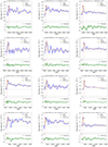 |
Fig. A.1. continued. |
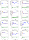 |
Fig. A.1. continued. |
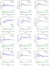 |
Fig. A.1. continued. |
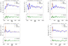 |
Fig. A.1. continued. |
All Tables
Physical and spectroscopic properties of the Lyα emitting galaxies in the CEERS sample.
Spearman correlation coefficients with the Lyα escape fraction for the Lyα emitting galaxies sample.
All Figures
|
Fig. 1. 1D spectra examples from the parent sample. Back solid line and green shaded region represent the flux and associated error respectively. For each galaxy, we report the emission line features spotted for the identification of the spectroscopic redshift. The position of the Lyα line is also highlighted. MSA ID = 44 and 1374 are Lyα emitters with S/N > 3, while MSA ID = 1023, 397, and 11 117 have no Lyα in emission. We report wavelengths in the rest-frame for clarity. |
| In the text | |
|
Fig. 2. Redshift distribution of the 150 sources (AGNs included) identified in CEERS and of the 91 galaxies presented in Jones et al. (2024) from the JADES survey. Lyα emitting galaxies with S/N > 3 from the combined sample are shown in dark grey. |
| In the text | |
|
Fig. 3. Spatial distribution of the 150 sources (AGNs included) spectroscopically-confirmed in CEERS. Blue (red) dots are galaxies that do (do not) show Lyα emission with S/N > 3. The AGNs are represented by the yellow dots. Green and orange squares represent the pointings for NIRCam and NIRSpec, respectively. The HST and JWST images of the field are shown in the background. |
| In the text | |
|
Fig. 4. Several examples of fitted Lyα emitters in the sample for different values of the emission line S/N. Left: MSA ID = 1561 with S/N = 23; Center: MSA ID = 439 with S/N = 7; Right: MSA ID = 1142 S/N = 3. In the upper panels, the blue solid line and shaded area denote the flux and error measurement as a function of the observed wavelength. The best fit-model is represented by an orange solid line, with the related |
| In the text | |
|
Fig. 5. EW0 distribution of the Lyα emitting galaxies in the combined CEERS + JADES sample. The red (blue) histogram shows the population at z < 6 (z > 6). The red (blue) solid line shows the best fit exponential declining distribution P(EW)∝e−EW0/W0 using EMCEE (Foreman-Mackey et al. 2013). The two populations are sampled in the range −21 < MUV < −17. |
| In the text | |
|
Fig. 6. Lyα EW0 versus MUV for our sample. Circles denote measured EW0 with S/N > 3, while triangles represent galaxies with just EW0, lim upper limits. CEERS data are color coded by redshift, while JADES galaxies are reported in grey for comparison. The black dashed lines (MUV = −20.25 and −18.75) divide the sample from the bright and faint ends. |
| In the text | |
|
Fig. 7. Lyα escape fraction as a function of rest frame Lyα equivalent width, stellar mass, UV absolute magnitude, reddening, UV β slope, and star formation rate. CEERS and JADES data are represented by circles and diamonds respectively. We report lower limits with black arrows, error bars are in grey instead. In the top-left panel, we show the fit relation found by Begley et al. (2024) in VANDELS z ∼ 4 − 5 data. In the middle-right panel, we show the best fitting relations found by Hayes et al. (2011), which exhibit a slight deviation from the trend proposed by Calzetti et al. (2000). |
| In the text | |
|
Fig. 8. Lyα escape fraction as a function of the LyC escape fraction inferred from the combination of spectroscopic properties using the relation derived by Mascia et al. (2024). Symbols are the same as in Fig. 7. The left panel includes all post-reionization galaxies (z < 5.5) while the right panel includes galaxies residing in a partially ionized IGM. For comparison, we report with the solid green line and region the best fitting relation found by Begley et al. (2024) for z ∼ 4 − 5 emitters. |
| In the text | |
|
Fig. 9. Lyα fraction as a function of redshift. Blue, red, and green data points represent CEERS, JADES, and the combined sample. The open data points are obtained when we do not consider the galaxies in the overdensity at z ∼ 7.18 and z ∼ 7.49. Error bars are calculated from the binomial statistics described in Gehrels (1986). The black bar is the result obtained with the CodaII simulation at z = 7. Grey symbols are taken from literature, we provide the full list here in the same order as the legend: Stark et al. (2011), Tilvi et al. (2014), De Barros et al. (2017), Mason et al. (2018b, 2019), Pentericci et al. (2018a), Fuller et al. (2020), Kusakabe et al. (2020), Goovaerts et al. (2023), Jones et al. (2024), and Nakane et al. (2024). Some of the points have been slightly shifted in redshift for an easier visualization. |
| In the text | |
|
Fig. 10. Ionized bubble at z = 7.18. Left: position of the five spectroscopically-confirmed galaxies in the z ∼ 7.18 reionized region. Blue stars are the three LAEs with S/N > 3 and the red stars are the non-emitting ones, while we show the four photometric candidates with grey circles. Right: predicted size of an ionized bubble as a function of time since ionizing radiation is switched on. Solid coloured lines are for individual sources while the black solid line and shaded region represent the predicted size of the ionized bubble carved by the 5 galaxies together. The horizontal dashed line represents the physical bubble radius. |
| In the text | |
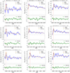 |
Fig. A.1. See the description of Fig. 4. |
| In the text | |
|
Fig. A.1. continued. |
| In the text | |
|
Fig. A.1. continued. |
| In the text | |
|
Fig. A.1. continued. |
| In the text | |
|
Fig. A.1. continued. |
| In the text | |
Current usage metrics show cumulative count of Article Views (full-text article views including HTML views, PDF and ePub downloads, according to the available data) and Abstracts Views on Vision4Press platform.
Data correspond to usage on the plateform after 2015. The current usage metrics is available 48-96 hours after online publication and is updated daily on week days.
Initial download of the metrics may take a while.