| Issue |
A&A
Volume 693, January 2025
|
|
|---|---|---|
| Article Number | A252 | |
| Number of page(s) | 36 | |
| Section | Extragalactic astronomy | |
| DOI | https://doi.org/10.1051/0004-6361/202451012 | |
| Published online | 27 January 2025 | |
The Lyman alpha reference sample
XV. Relating ionised gas kinematics with Lyman-α observables
1
Inter-University Centre for Astronomy and Astrophysics (IUCAA), Pune University Campus, Pune 411 007, India
2
Universität Heidelberg, Interdisziplinäres Zentrum für Wissenschaftliches Rechnen, Im Neuenheimer Feld 205, D-69120 Heidelberg Germany
3
, Universität Heidelberg, Zentrum für Astronomie, Institut für Theoretische Astrophysik, Albert-Ueberle-Straße 2, D-69120 Heidelberg, Germany
4
Cosmic Dawn Center (DAWN), Copenhagen, Denmark
5
Niels Bohr Institute, University of Copenhagen, Copenhagen, Denmark
6
Department of Astronomy, Stockholm University, AlbaNova University Centre, SE-106 91, Stockholm, Sweden
7
Minnesota Institute for Astrophysics, University of Minnesota, 116 Church Street SE, Minneapolis, MN 55455, USA
8
Department of Physics & Astronomy, Macalester College, 1600 Grand Avenue, Saint Paul, MN 55105, USA
9
Leibniz Institute for Astrophysics (AIP), An der Sternware 16, 14482 Potsdam, Germany
⋆ Corresponding author; This email address is being protected from spambots. You need JavaScript enabled to view it.
Received:
6
June
2024
Accepted:
11
September
2024
Abstract
Gas kinematics affect the radiative transfer and escape of hydrogen Lyman-α (Lyα) emission from galaxies. We investigate this interplay empirically by relating the ionised gas kinematics of 42 galaxies in the extended Lyα Reference Sample (eLARS) with their Lyα escape fractions, fescLyα, Lyα equivalent widths, EWLyα, and Lyα luminosities, LLyα. To this aim we use PMAS integral-field spectroscopic observations of the Balmer-α line. Our sample contains 18 rotating discs, 13 perturbed rotators, and 13 galaxies with more complex kinematics. The distributions of fescLyα, EWLyα, and LLyα do not differ significantly between these kinematical classes, but the largest Lyα observables are found amongst the kinematically complex systems. We find no trends between either fescLyα or EWLyα and kinematic or photometric inclinations. We calculate shearing velocities, vshear, and intrinsic velocity dispersions, σ0obs (empirically corrected for beam-smearing effects), as global kinematical measures for each galaxy. The sample is characterised by highly turbulent motions (30 km s−1 ≲ σ0obs ≲ 80 km s−1) and more than half of the sources show dispersion-dominated kinematics. We uncover clear trends between Lyα observables and global kinematical statistics: EWLyα and LLyα correlate with σ0obs, while fescLyα anti-correlates with vshear and vshear/σ0obs. Moreover, we find, that galaxies with EWLyα ≥ 20 Å are characterised by higher σ0 and lower vshear/σ0obs than galaxies below this threshold. We discuss the statistical importance of vshear, σ0obs, and vshear/σ0obs for regulating the Lyα observables in comparison to other galaxy parameters. It emerges that σ0obs is the dominating parameter for regulating EWLyα and that is as important as nebular extinction, gas covering fraction, and ionising photon production efficiency in regulating fescLyα. A simple scenario where the starburst age is simultaneously regulating turbulence, EWLyα, and fescesc is not supported by our observations. However, we show that the small-scale distribution of dust appears to be influenced by turbulence in some galaxies. In support of our observational result, we discuss how turbulence is theoretically expected to play a significant role in modulating fescLyα.
Key words: radiative transfer / galaxies: ISM / galaxies: kinematics and dynamics / galaxies: starburst
© The Authors 2025
 Open Access article, published by EDP Sciences, under the terms of the Creative Commons Attribution License (https://creativecommons.org/licenses/by/4.0), which permits unrestricted use, distribution, and reproduction in any medium, provided the original work is properly cited.
This article is published in open access under the Subscribe to Open model. This email address is being protected from spambots. You need JavaScript enabled to view it. to support open access publication.
1. Introduction
Studying the early stages of galaxy formation is fundamental for understanding their evolution and diversity in general. This requires observations of the most distant galaxies. Although the field has recently been revolutionised with the launch of the James Webb Space Telescope (JWST), galaxies in these early phases still appear as very faint and close-to-unresolved sources. While JWST has provided rest-frame optical emission line detections out to redshifts z ∼ 7 − 11 (e.g. Bunker et al. 2023; Arrabal Haro et al. 2023; Heintz et al. 2024; Saxena et al. 2023; Tang et al. 2023; Boyett et al. 2024), the rest-frame ultraviolett Lyman-α line (Lyα; λLyα = 1215.68 Å) remains of interest for galaxies in the early universe (see reviews by Hayes 2015; Dijkstra 2019; Ouchi et al. 2020). Originating mainly from the recombining gas in the vicinity of hot O- and B-stars, Lyα is associated in particular with young galaxies that are in the process of rapidly converting gas into stars, as famously envisioned by Partridge & Peebles (1967).
An observational census of Lyα-emitting galaxies (LAEs) has been established for galaxies with Lyα luminosities of LLyα ≳ 1041.5 erg s−1 throughout most of the history of the Universe (e.g., Ouchi et al. 2008; Blanc et al. 2011; Sobral et al. 2018; Wold et al. 2017; Herenz et al. 2019; Liu & Jiang 2023; Thai et al. 2023) up until the epoch of reionisation (EoR; e.g., Ouchi et al. 2010; Matthee et al. 2015; Santos et al. 2016; Konno et al. 2018; Ning et al. 2022; Wold et al. 2022) by means of the LAE luminosity function. These censuses ascertain that LAEs are an abundant population of high-redshift (z ≳ 2) galaxies that can serve as a tracer for addressing fundamental questions of galaxy formation and cosmology. For example, the HETDEX survey will measure redshifts of more than a million LAEs from z ∼ 1.8 to z ∼ 2.5 to investigate the nature of dark energy (Gebhardt et al. 2021; Mentuch Cooper et al. 2023). Moreover, LAEs also serve as an important probe to constrain the timeline and the topology of the intergalactic medium during the EoR (e.g. reviews by Dijkstra 2014 and Choudhury 2022; see also recent results by Nakane et al. 2024, Witstok et al. 2024, and Witten et al. 2024). Finally, large-area cosmological line-intensity mapping experiments that attempt to measure baryonic acoustic oscillations as a function of the age of the Universe will also rely on the Lyα signal from the unresolved population of LAEs (e.g. Bernal & Kovetz 2022; Lujan Niemeyer et al. 2023).
Given the high Lyα absorption cross-section of neutral hydrogen, the resulting Lyα optical depths in typical interstellar media (ISM) are extremely high (τLyα > 106 for neutral columns of NHI > 1020 cm−2). Hence the Lyα line is resonant. The resulting complex radiative transfer within the ISM redistributes the initial Lyα radiation field spatially and in frequency space. Moreover, the radiative transfer increases a Lyα path length of the photon and makes it prone to absorption by dust. Theoretical works demonstrate the resulting intricate relationships between Lyα observables (e.g. Lyα spectral morphology, Lyα surface brightness distribution, and total Lyα line intensity) and the density distribution, dust distribution, and kinematics of the interstellar scattering medium (see, e.g. recent papers by Remolina-Gutiérrez & Forero-Romero 2019; Smith et al. 2019; Lao & Smith 2020; Song et al. 2020; Gronke et al. 2021; Li et al. 2022; Blaizot et al. 2023; Munirov & Kaurov 2023, and references therein).
A key quantity in the context of LAEs is the Lyα escape fraction,  , which is defined as the ratio between the observed Lyα luminosity and the intrinsic Lyα luminosity. An understanding of the galactic characteristics that regulate
  is required to answer the question of what makes a star-forming galaxy an LAE. Many observational (e.g., Giavalisco et al. 1996; Keel 2005; Finkelstein et al. 2009; Hayes et al. 2011; Malhotra et al. 2012; Atek et al. 2014; Hathi et al. 2016; Hagen et al. 2016; Oyarzún et al. 2016; Paulino-Afonso et al. 2018; Matthee et al. 2021; McCarron et al.2022; Chávez Ortiz et al. 2023; Napolitano et al. 2023; Hayes et al. 2023; Lin et al. 2024) and modelling (e.g. Schaerer & Verhamme 2008; Verhamme et al. 2008; Forero-Romero et al. 2011; Dijkstra & Wyithe 2012; Dayal & Libeskind 2012; Garel et al. 2015, 2016; Gurung-López et al. 2019) efforts have been conducted with the intention of answering this question. It is now established that the physical and morphological characteristics of LAEs are significantly different from star-forming galaxies where
  ∼ 0. As reviewed by Ouchi et al. (2020), high-z LAEs are commonly compact (re ∼ 1 kpc) star-forming galaxies (SFR ∼ 1…10 M⊙yr−1) with low-dust content (E(B − V)≲0.2) that harbour young stellar populations (age ∼ 10 Myr) of low stellar mass (∼108…109 M⊙). Moreover, the ISM of those galaxies is often metal poor, with metallicities ranging from Z ∼ 0.1 Z⊙ to Z ∼ 0.3 Z⊙. This differentiates LAEs from non-LAEs and/or continuum-selected high-z galaxies, which are typically more evolved and more massive systems, but there is certainly overlap between the two populations.
The defining criterion for LAEs in surveys is often based on a threshold in the equivalent width of the Lyα line, EWLyα. Interestingly, EWLyα is linearly correlated with  (Sobral & Matthee 2019; Melinder et al. 2023). Sobral & Matthee (2019) explain the measured slope of this relation in a simple scenario where, on average, galaxies with higher EWLyα and
  are dominated by stellar populations with a harder ionising spectrum, as characterised by the ionising photon production efficiency ξion, and lower E(B − V). This idea is consistent with results that show how the overall dust-poor high-EWLyα LAEs are indeed characterised by higher ξion (e.g., Trainor et al. 2016; Nakajima et al. 2016, 2018; Maseda et al. 2020; Hayes et al. 2023; Kramarenko et al. 2024). Certainly, ξion and E(B − V) are galaxy characteristics that we expect to directly influence the radiative transfer. The fact that these characteristics occur predominantly in compact star-forming systems of low metallicity and low mass informs us more about the processes of star formation and, more generally, galaxy formation physics in such systems. However, the causal connection between Lyα radiative transport physics and stellar mass or star-formation rate appears to involve some other process. In this respect we reiterate that galaxy and ISM kinematics are causally connected with star formation and stellar mass (see e.g. review by Glazebrook 2013). Thus we may also expect also causal relationships between galaxy kinematics and/or
  or EWLyα.
Significant effort has been devoted to understanding the effect of kinematics and gas distribution on the Lyα line profile morphology (e.g., Blaizot et al. 2023, and references therein). The kinematics of the scattering medium are also frequently studied in absorption, especially using low-ionisation-state absorption lines of Si+ and C+ ions in the UV (Kunth et al. 1998; Wofford et al. 2013; Henry et al. 2015; Rivera-Thorsen et al. 2015; Hayes 2023; Hayes et al. 2023). These line-profile analyses and absorption-line studies reveal how low-neutral-H I covering fractions and outflow kinematics appear to promote Lyα escape. In principle, the neutral phase can also be probed by the 21 cm line. However, the spatial resolution of the radio beam is usually significantly lower then the spatial scales that can be probed by imaging and spectroscopy (Cannon et al. 2004; Pardy et al. 2014). Nevertheless, such analyses reveal that mergers offset large amounts of H I via tidal interactions and it appears likely that the thereby reduced neutral column towards the star-forming regions promotes Lyα escape (Purkayastha et al. 2022; Le Reste et al. 2024). A promising way forward comes in the form of highly spatially resolved aperture-synthesis observations in combination with other observational probes of the emitting and scattering medium. Especially recent work by Le Reste et al. (2022) informs us about the role of the interplay between H II and H I gas on ISM scales in facilitating Lyα escape.
To date, few studies have sought to understand the role of gas kinematics in shaping the global Lyα characteristics  , EWLyα, and Lyα luminosity (LLyα). To this aim we must leverage galaxy-averaged kinematical statistics. Importantly, this averaging should be done on spatial scales most relevant for the radiative-transfer problem. Such an analysis was attempted by Herenz et al. (2016), hereafter H16, who used integral-field spectroscopic observations of the Hα line of the Lyman-α reference sample (LARS; Östlin et al. 2014). This study found that, galaxies whose ionised gas kinematics are dominated by unordered (turbulent) motions can appear as Lyα emitters, whereas galaxies that are dominated by large-scale coherent motions never appear to show significant Lyα escape. Evidence for turbulence-driven Lyα escape was also presented by Puschnig et al. (2020) from a study of the dust and the molecular gas content of LARS. Moreover, a connection between global galaxy kinematics and Lyα escape was reported very recently by Foran et al. (2024) for the first time in high-z galaxies. These authors analysed the global kinematical characteristics of z ∼ 2 and z ∼ 3 galaxies for which consistent EWLyα measurements were available. Objects that showed no significant Lyα emission or even Lyα in absorption (i.e. low or negative EWLyα) were found to be a mixture of dispersion- and rotation-dominated systems, whereas galaxies with significant Lyα emission were always found to be dispersion dominated.
The goal of the present study is to revisit the relationship between galaxy kinematics and Lyα characteristics observationally, with the main aim being to remove the shortcomings of the rather small sample used in the kinematical study of H16. To this aim, we analysed integral-field spectroscopic observations of the Hα line for all 42 galaxies of the LARS + extended LARS programmes (eLARS; Melinder et al. 2023, herafter M23). The enlarged dataset now allows us to discuss the importance of galaxy kinematics for Lyα observables with respect to other galaxy characteristics in a quantitative manner.
This paper is structured as follows: Section 2 describes the sample and data, especially the newly obtained Calar-Alto 3.5m PMAS observations. Section 3 presents the kinematic analysis and our relations between galaxy kinematics and Lyα observables. Section 4 then discusses the importance of kinematic parameters with respect to the “soup of quantities” that have been found to correlate with Lyα properties of galaxies. An astrophysical interpretation of the results is also presented in Sect. 4. Finally, Sect. 5 concludes this paper.
2. Data
2.1. The (Extended) Lyman-α Reference Sample
The sample analysed here consists of 42 star-forming galaxies selected from the SDSS spectroscopic database. The main selection criteria are cuts in the Hα equivalent width, EWHα (as a proxy for stellar age), and FUV luminosity (at λ ≈ 1500 Å from GALEX), LUV (as a proxy for star-formation rate). Fourteen of the 42 galaxies had to satisfy a cut in EWHα > 100 Å. These 14 galaxies (LARS1 – LARS14) comprised the initial Lyα Reference Sample (LARS; Östlin et al. 2014; Hayes et al. 2014). As detailed in Östlin et al. (2014), additional considerations for the sample selection were that the galaxies cover a range in FUV luminosities typical of star-forming galaxies in the early universe, and the availability of relevant Hubble Space Telescope (HST) archival data to design the HST imaging and spectroscopic campaign as economically as possible.
The initial sample was extended with 28 star-forming galaxies (eLARS 1–28) that had to satisfy a cut of EWHα > 40 Å, and again the sample was picked to include a dynamical range in LUV (M23). Only 7 out of those 28 galaxies show EWHα > 100 Å. The final sample, LARS+eLARS, now spans a range in log10(LFUV [L⊙]) from 9 to 11 and in EWHα from 41 Å to 578 Å. Stellar mass and Hα star-formation rate distributions are presented in Sect. 3.5. All galaxies show emission line ratios consistent with being powered by a young stellar population according to the extreme starburst classification demarcation line in the [O III]λ5007]/Hβ vs. [N II]λ6548/Hα diagram provided by Kewley et al. (2001). However, five galaxies could be classified as harbouring an AGN according to the criterion of Kauffmann et al. (2003). The HST imaging observations of all 42 galaxies were used to synthesise images in Lyα, Hα, and Hβ. We use for the present analysis global measurements derived from these images (see Sect. 2.4 below).
2.2. PMAS observations of eLARS
We observed all 28 eLARS galaxies with the Potsdam Multi Aperture Spectrophotometer (PMAS; Roth et al. 2005) at the Calar Alto 3.5 m telescope. An overview of the campaign is provided Table A.1 of Appendix A. We used PMAS in its Lens Array configuration with double magnification – in this configuration the 256 spectral pixels (spaxels) of 1″×1″ size sample contiguously a 16″×16″ field of view. Within this field of view the bulk of the high surface-brightness Hα emission of the galaxies in the sample could be covered with a single pointing. Exceptions are eLARS 3, 5, and 26, which required two pointings (pointings are differentiated by the suffixes A and B in Table A.1). We used the R1200 backward-blazed grating as in H16, but different to H16, here the grating angle could be held fixed so to disperse the first spectral order around Hα close to the centre of the detector for all galaxies. According to the PMAS grating table1 the expected nominal resolving power for the adopted position (GROTPOS = 109) is R ∼ 5000. In order to sample the spectroscopic line spread function adequately at this resolving power (see Robertson 2017) we did not bin the read out of the PMAS 4k×4k CCD along the dispersion direction (XBIN = 1). This set up was chosen to obtain data that is optimal for a kinematic study of the ionised gas.
The observations took place during the course of two visitor mode observing runs in spring 2016 (run350) and spring 2017 (run362). We observed all our targets at air-masses ≲1.3. The observing conditions were not always optimal, with mediocre seeing and occasional thick cloud cover. Nevertheless, by visually monitoring the incoming read outs of the PMAS 4k×4k CCD after each exposure, we ensured that there is sufficient signal in the Hα lines that could be used for our analysis. Observations that did not contain enough signal due to cloud cover were repeated. If the conditions permitted, we took an additional 400s blank sky exposure close to the target. We ensured that such blank sky exposures were always taken when the redshifted Hα line was in spectral proximity to a bright telluric line. Sky flat exposures were taken at the beginning or end of each night. On-sky exposures were always flanked by a continuum lamp exposure and an arc-lamp exposure (HgNe).
Due to strong ambient temperature fluctuations the spectrograph was not always optimally focused. Thus, especially during the 2016 run, sometimes lower values of R are measured (see Table A.1 – the resolving power determination and correction is described in Appendix B). Fortunately, the galaxy’s Hα profiles are always resolved significantly, also in the slightly suboptimal R ∼ 3000 datasets.
We reduced the observational raw data with the general reduction pipeline for fibre-fed integral-field spectrographs p3d (Sandin et al. 2010, 2012). Our reduction strategy is detailed in Sect. 3 of H16, and for completeness we provide a summary in Appendix A.
2.3. The original LARS PMAS data
In this study, we combine our new observational results with the results from our study of Hα kinematics in the original LARS sample H16. The LARS datacubes are available via the CDS2. In the following we reanalyse these LARS datacubes with the methods used for the eLARS observations presented in Sect. 3.1 and described in detail in Appendix B. While there are slight quantitative differences in the recovered velocity fields and velocity dispersion maps (see Sect. 3.3), their visual appearance is not significantly different from what was presented in H16. Thus, we streamline the presentation here by not presenting those maps again; the interested reader is referred to Figs. 5–7 in H16.
2.4. Global measurements from HST imaging
For relating the ionised gas kinematics with the galaxies physical parameters (stellar mass M⋆, star-formation rate SFRHα, starburst age) and their Lyα observables (equivalent width EWLyα, escape fraction  , and observed Lyα luminosity, LLyα) we rely on the integrated measurements provided in M23. As described there in detail, the required global quantities were measured within circular apertures on Voronoi-binned maps that were created from UV and optical PSF-matched HST imaging data that was processed with an updated version LaXs pipeline (Hayes et al. 2009). The radii of these apertures, denoted rtot in M23, are defined on the Lyα maps, as Lyα is often more extended then Hα or the FUV continuum. The EWLyα is defined as the ratio between the aperture integrated Lyα luminosity and the UV continuum luminosity at λLyα, and
  is defined as
 (1)
(1)
where k(λHα) is the extinction coefficient at the wavelength of Hα, and E(B − V) is the aperture integrated colour excess that attenuates nebular emission and is derived from the Balmer-decrement,
 (2)
(2)
using the integrated luminosities derived from the reconstructed Hα and Hβ images. The intrinsic ratios of Lyα / Hα and Hα/Hβ luminosities are given by the canonical Case-B recombination values (LLyα/LHα)int = 8.7 (see, e.g. Fig. 4.2 in Hayes 2015) and (LHα/LHβ)int = 2.86, respectively. Moreover, M23 use the Cardelli et al. (1989) extinction curve for k(λ)3 in Eq. (1) and Eq. (2). Nebular extinction is thus assumed to be caused by a homogeneous dust screen in front of the line emitting gas.
We note that no significant Lyα emission could be detected for six galaxies in the sample (LARS 6, LARS 10, LARS13, ELARS 12, ELARS 14, and ELARS 16). Hence, these galaxies only have upper limits in their Lyα observables. Furthermore, we note that M23 performed a refined and more accurate reprocessing of the HST imaging data also for the 14 galaxies constituting the original LARS sample. Hence, the global Lyα luminosities, equivalent widths, and escape fractions are different and supersede the values presented in Hayes et al. (2014) and Runnholm et al. (2020). Adopting the a cut of EWLyα ≥ 20 Å to define a galaxy as LAE, the sample contains 12 LAEs.
3. Analysis
3.1. Line-of-sight velocity and velocity dispersion maps
We project the kinematical properties traced by Hα in the IFS cuboids into 2D maps of line-of-sight velocity vlos and velocity dispersion σv. Our procedures for creating the S/N, vlos, and σv maps closely follow the well established convention for this task that involves fitting single-component Gaussian profiles to the continuum subtracted data (e.g. Alonso-Herrero et al. 2009). We describe the creation of the maps in more detail in Appendix B.
We here note that only for the galaxies eLARS 7 and eLARS 24 numerous spaxels are not well described by a single Gaussian component. The spectral profile in those spaxels show strong bimodality indicating the projection of two distinct kinematic components along the line of sight4. Thus the width and position of the Gaussian fits becomes unreliable parameters. A similar situation is also encountered in LARS 9 and LARS 13 from the H16 sample. All four galaxies with double component profiles are excluded in the following statistical analyses involving velocity dispersion measurements.
We show the vlos and σv maps alongside their signal-to-noise maps (S/N) in Hα for four eLARS galaxies in Fig. 1; Fig. B.1 in Appendix B provides those maps for the full sample. An atlas that allows for a visual comparison between the HST imaging data with the kinematical maps is presented in Appendix A.1 of Schaible (2023). To the best of our knowledge, kinematic maps of the ionised phase of the galaxies analysed in this study have not been presented elsewhere, with the exception being eLARS 1, for which Hα kinematics from scanning Fabry-Perot observations were analysed in Sardaneta et al. (2020).
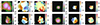 |
Fig. 1. Hα kinematics of four eLARS galaxies from PMAS (16″ × 16″ field of view). For each galaxy we show HαS/N (left panels; colour coded in log-scale from 1 to 1000), vlos [km s−1] (centre panels; velocities are colour coded linearly from blue (approaching) to red (receding) with the centre at vlos = 0 in white and scaled symmetrically to the absolute maximum), and σv [km s−1] (right panels; colour coded linearly from the 2nd percentile to the 98th percentile of the observed σv distribution per galaxy). The name of each galaxy is coloured according to the visual kinematic classification (Sect. 3.2): rotating discs in purple, perturbed rotators in green, and galaxies with complex kinematics in orange. The full sample is shown in Appendix B (Fig. B.1). |
3.2. Visual classification of the velocity fields
3.2.1. Classification scheme and results
We visually characterise the vlos maps shown in Fig. B.1 according to three qualitative kinematical categories (see review by Glazebrook 2013): “rotating disc” (RD), “perturbed rotator” (PR), and “complex kinematics” (CK).
For RD galaxies the bulk of the Hα emitting gas needs to be dominated by orbital motion. The resulting velocity field shows a smooth gradient which steepens in the centre and this gradient is aligned parallel to the major axis of the optical image. Projection of a galaxy’s differential rotation lead to a classical symmetric “spider-leg” morphology of observed iso-velocity contours (not shown here; see, e.g. Fig. 8 in Gnerucci et al. 2011 or Fig. 6 in Epinat et al. 2010 for examples). Importantly, the receding and approaching velocities mirror each other. Moreover, for RD galaxies the velocity dispersion map often show elevated σv values near the kinematical centre (the reasons for this are provided in Appendix C). The velocity fields of PR galaxies are still dominated by orbital motions, but they show significant deviations from a perfect disc. Lastly, galaxies characterised by CK exhibit no clear gradient indicative of simple orbital motions. For CK galaxies the gradient also appears less steep in comparison to RDs or PRs.
This visual classification is certainly subjective as there is a not a well defined boundary between the classes. Hence, the classification was done by six authors individually (ECH, AS, PL, MH, ALR, and GÖ) and then finalised in a consolidation session. Moreover, as described in detail in Appendix C.1 the classification of the RDs is confirmed by successfully modelling the RD systems by simple disc models with GalPak3D (Bouché et al. 2015) and by the symmetric appearance of the line-of-sight velocity profiles along the kinematical major axis (Appendix C.2; Fig. C.3). The classifications for the combined LARS and eLARS sample are listed given in Appendix D (Table D.1). Moreover, we colour the label of each galaxy in Fig. B.1 according to its kinematical class.
According to our visual classification, the eLARS sample contains 4 CK galaxies (14% of eLARS), 8 PR galaxies (29% of eLARS), and 16 RD galaxies (57% of eLARS). This is different compared to the original LARS sample, where 7 galaxies have complex kinematics (50% of LARS), 5 are a PR (36% of LARS), and only 2 are a RD (14% of LARS). This difference is a consequence of the sample selection. Whereas LARS galaxies had to satisfy an Hα equivalent width cut of EWHα ≥ 100 Å, this requirement was lowered to EWHα ≥ 40 Å for eLARS to remove the bias towards irregular and merging systems M23, which are characterised by CK. The combined sample of all 42 eLARS and LARS galaxies consists of 18 (43%) RD galaxies, 13 (31%) PR galaxies, while 11 (26%) galaxies of the sample exhibit CK.
This almost three-way split amongst the kinematical categories bears resemblance to the split found in early IFU studies of star-forming galaxies at similar masses in the high-z (z ≳ 1) universe (Glazebrook 2013, and references therein). More recent surveys, which use stricter criteria to define rotating discs, report disc fractions in excess of 50 % (Wisnioski et al. 2015, 2019), but that could be an overestimate due to mergers acting as disc impostors (Simons et al. 2019).
3.2.2. Comparing Lyα observables between kinematical classes
We may imagine that interstellar medium conditions in galaxies with complex velocity fields are favourable for Lyα escape. For example, irregular and merging systems are often characterised by high specific SFRs, which lead to spatially concentrated injection of momentum and energy from stellar feedback processes. The resulting winds and outflows then may lead to a more effective clearing of escape channels for Lyα (and also Lyman continuum) radiation. The 42 galaxies of the combined LARS and eLARS sample allow for a statistical exploration of such a scenario.
We begin by showing stacked histograms of the Lyα observables colour-coded by their kinematical class in our sample in Fig. 2. The maximum EWLyα (56.7 Å; LARS 2), maximum  (0.3; LARS 2), and maximum LLyα (5.6 × 1042 erg s−1; LARS 14) values are found indeed among the CK objects. Moreover, also the averages of those observables are larger in the CK class (⟨EWLyα⟩ = 23.15 Å: ⟨
 ⟩ = 0.102; ⟨LLyα⟩ = 1.02 × 1042 erg s−1) than the averages found for the PR (⟨EWLyα⟩ = 17.47 Å; ⟨
 ⟩ = 0.067; ⟨LLyα⟩ = 2.75 × 1041 erg s−1) and for the RD (⟨EWLyα⟩ = 16.36 Å; ⟨
 ⟩ = 0.057; ⟨LLyα⟩ = 3.10 × 1041 erg s−1) galaxies, respectively. However, also non-detections of Lyα emission are found amongst objects in all three classes.
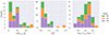 |
Fig. 2. Stacked histograms, colour coded according to kinematical class (rotating discs: purple; perturbed rotators: green; complex kinematics: orange) of the Lyα observables EWLyα (left panel), |

In order to quantify the difference of the observed distributions of Lyα observables amongst the different classes we use the two-sample Kolmogorov-Smirnov (KS) test. Here the six galaxies with upper limits in their Lyα observables are excluded from calculating the KS-test statistic. As mentioned in Sect. 3.2.1, the boundary between our three classes is not well defined, and some PRs could also be classified either as CKs or RDs. For the KS-test we thus regroup our sample into two groups, 𝒜 and ℬ. First, we combine the RDs and PRs into group 𝒜 (27 galaxies) and the CKs into group ℬ (9 galaxies), then we associate only the RDs with group 𝒜 (15 galaxies) and combine the PRs with the CKs in group ℬ (21 galaxies). For both parings and for all three Lyα observables the KS-test is consistent with the null-hypothesis that the samples in the kinematic class are drawn from the same parent population (p-values in the range pKS ∼ 0.2…0.3). This exercise shows that there is significant overlap in the Lyα observables amongst the kinematical classes. The qualitative nature of a galaxy’s line-of-sight ionised gas velocity field in our sample does not reflect whether it is as a strong Lyα emitter or not.
3.3. Global kinematical measures: vshear, σ0obs, and σtot
We now turn to a more quantitative analysis of the observed line-of-sight velocity- and velocity dispersion maps. Therefore we derive two main summarising measures from those maps: the apparent shearing velocity, vshear, and the intrinsic velocity dispersion, σ0 (see review by Glazebrook 2013).
For the calculation of vshear we account for extreme outliers from the distribution of observed velocities. To this aim we calculate  for each galaxy, with vmax and vmin being the values of the 95th percentile and the 5th percentile of the vlos values, respectively. The upper- and lower errors on vlos are estimated from the difference of the 95th and 5th percentiles, respectively, to the mean of the values outside of each percentile.
For σ0 we adopt the notion of a galaxy’s average line-of-sight velocity dispersion. This simplistic definition implicitly assumes that the σ0 is isotropic. For measuring this quantity from the observed dispersion fields we need to account for inflated values in individual spaxels due to the convolution of the galaxies’ intrinsic Hα spatial- and spectral- morphology with the atmospheres point spread function and the coarse sampling by 1″×1″ spaxels. In H16 we made no such correction, but the large fraction of RD galaxies in the combined LARS+eLARS sample demands us to be more cautious in this respect. Various methods that attempt to correct for this “beam smearing” or, more correctly, “point-spread function smearing” effect have been presented in the literature (e.g. Davies et al. 2011; Varidel et al. 2016). We compare several such methods against results from morphokinematical modelling of our observations with the GalPaK3D software (Bouché et al. 2015) in Appendix C. This modelling accounts for the spectral and spatial convolution of the observed Hα kinematics and it adopts also the notion that σ0 is isotropic. However, GalPak3D can only be applied to rotating systems. Given the large fraction of more complex systems in our sample we thus require an empirical method for estimating σ0 directly from the data. In Appendix C we find that the model-based velocity dispersions can be reliably recovered by averaging the σv maps, provided that certain spaxels are masked according to a local gradient-measure in the vlos map. The uncertainty on  is calculated by propagating the Δσ0’s of the individual spaxels (Sect. 3.1) in quadrature.
The vshear and  values as determined above are listed in Table D.1 of Appendix D. We comment that there is a small difference between the vshear values reported for the LARS galaxies in H16 and the values listed here. This difference is because H16 applied a Voronoi-binning technique to the datacube, whereas here we use each spaxel as is. Moreover, we here used the intervals outside the 95th and 5th percentiles individually to estimate the uncertainty, whereas H16 symmetrised the error-bars. That being so, the here reported updated vshear measurements and error estimates agree within the error-bars of H16. In contrast, the here tabulated
  values were computed more thoroughly as explained above (see also Appendix C) and are thus slightly different.
We find maximum shearing velocities in eLARS 3 ( km s−1) and LARS 13 (
 km s−1), with the former being a rotating disc and the latter being a merger that exhibits complex kinematics. Minimum shearing velocities are observed in eLARS 28 (
 km s−1) and LARS 2 (
 km s−1), a perturbed rotator and a complex system, respectively. In Fig. 3 (left panel) we show a stacked histogram of vshear colour-coded by kinematical class. We note that the distribution of the RDs differs markedly in comparison to the PRs and CKs, with the latter two classes showing overall lower vshear values. Despite the eLARS extension enlarging the fraction of discs compared to LARS, only one new vshear extremum is introduced into the combined sample (eLARS 03). Thus, we now sample the vshear range at hand more densely, as reflected also by the mean and the median of vshear (57.96 km s−1 and 73.13 km s−1, respectively) being similar or identical to the respective values of the original LARS sample (52.4 km s−1 and 73.13 km s−1). Given that the selection of our sample is limited to young star-bursts, the shearing velocities in our sample are unsurprisingly lower than what is observed for more massive disc galaxies, even when not corrected for inclination.
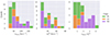 |
Fig. 3. Stacked histograms of the global kinematical measures vshear (left panel), |

For the velocity dispersions the maxima are observed in eLARS 24 (σ0obs = 78.0 ± 2.9 km s−1) and LARS 3 (σ0obs = 77.3 ± 2.9 km s−1) and the minima are seen in eLARS 16 (σ0obs = 23.9 ± 0.9 km s−1) and eLARS 23 (σ0obs = 23.9 ± 0.7 km s−1). We show a stacked histogram of  , colour coded by kinematical class, in Fig. 3 (middle panel). There appears not much difference regarding the distributions of
  in the different kinematical classes, except that most of the lowest velocity dispersions are found amongst the RDs and PRs. The eLARS extension introduces a larger fraction of lower velocity dispersion (σ0obs ∼ 35 km s−1) galaxies into the sample; this is apparent from Table D.1, and can also be seen by comparing mean and median
  of the full sample (41.1 km s−1 and 37.3 km s−1) to the original sample (55.6 km s−1 and 51.9 km s−1). The on average lower
  values are again a consequence of the lower EWHα cut used to define the extended sample (cf. Sect. 3.2.1). This is due to the fact that EWHα traces specific SFR (sSFR = SFR per galaxy mass), which tightly correlates with SFR (τ = 0.51, pτ ∼ 10−6 for LARS+eLARS; see also analysis by Law et al. 2022), and since the latter, as discussed already in the introduction, tightly correlates with SFR. This is analysed further Sect. 3.5 below.
We also use the ratio vshear/σ0obs that combines the above measurements to a summarising statistic of a galaxy’s kinematical state. These ratios are also listed in Table D.1. The asymmetric error-bars on vshear were propagated into vshear/σ0obs after moving into log-space and then using method presented in the appendix of Laursen et al. (2019). Our sample is characterised by low vshear/σ0obs values, ranging from 0.35 to 4.46 (median: 1.6, average: 1.8). We show the corresponding stacked-histogram with colour coding by kinematical class in the right panel of Fig. 3. The distributions of vshear/σ0obs differ markedly when comparing the RDs with the CKs and PRs, with the later clearly dominating the low- vshear/σ0obs range. Still, the overall low ratios in the whole sample are below that of typical disc galaxies (vrot/σ0 ≳ 8, where vrot is the maximum rotational velocity; e.g. Epinat et al. 2008) and are more akin to low-mass star-forming galaxies at low- and high-redshifts. Galaxies with  can be classified as dispersion dominated galaxies, as here the turbulent motions exceed the value that would correspond to equal contributions of random motions and rotation to the dynamical support of a turbulent disc (Förster Schreiber & Wuyts 2020; Bik et al. 2022). According to this criterion 24 of the 42 galaxies in LARS+eLARS are dispersion dominated; most of these are PRs or CKs.
We again note that vshear is not inclination corrected, because such a correction is often ill-defined for the non-rotating complex systems. Thus, strictly speaking, vshear/σ0obs characterises the projected kinematical state. However, we argue that this projected kinematical state, rather than the inclination corrected ratio, is the relevant parameter for relating kinematics with Lyα observables. Especially for disc galaxies the Lyα escape fraction is theoretically expected to be strongly inclination dependent, with edge-on systems having absorbed most of the Lyα photons along the line of sight whereas a face-on system may show higher escape fractions (Laursen & Sommer-Larsen 2007; Laursen et al. 2009b; Behrens & Braun 2014; Verhamme et al. 2012; Smith et al. 2022). At comparable masses, this could lead to an anti-correlation between vshear/σ0obs and  for disc galaxies, since face-on discs should have preferentially lower vshear/σ0obs. A deprojected ratio could not trace such types of relations that are the subject of this study. We analyse the inclination dependence on the Lyα observables further in Sect. 3.4.
3.4. Inclination dependence on Lyα escape
To date the most detailed Lyα radiative transfer simulations were carried out for massive disc galaxies (Behrens & Braun 2014; Verhamme et al. 2012; Smith et al. 2022). These single galaxy simulations found a strong inclination dependence of EWLyα and  (see also Laursen & Sommer-Larsen 2007). The highest EWLyα and
  are found when the simulated galaxies are seen face-on, whereas Lyα is significantly extinguished when the galaxies are viewed edge-on. A plausible conjecture from those simulation results is that high-z samples selected on Lyα emission might be biased towards face-on systems. However, observational results on high-z LAEs, which use the photometric major- to minor axis ratio, b/a, or the flattening, 1 − b/a, as proxy for the inclination (since cos(i) = b/a for infinitely thin discs), are not supportive of this idea (Gronwall et al. 2011; Shibuya et al. 2014; Paulino-Afonso et al. 2018).
In the present contribution, we are equipped with kinematical inclinations, i, from the GalPak3D disc modelling of the 15 RDs that was performed to verify the empirical masking technique for the calculation of  (Appendix C.1). We list cos(i) in Table D.1. We compare these measurements to the photometric ratio determined in the I-band by Rasekh et al. (2022), as this quantity minimises the mean difference between photometric axis ratios and kinematic inclinations (⟨cos(i)−(b/a)⟩ = 0.07). Of course, no perfect match is expected, given that the simple approximation cos(i)≈b/a does not account for the finite thickness of the disc. Thus the photometric inclination is biased low for systems that are observed close to edge-on; LARS 11 and eLARS 18 are such cases in our sample. Moreover, Rasekh et al. (2022) calculate the axis ratio from the image moments. However, these measures are sensitive to substructures (i.e. clumps and spiral arms) that are not homogeneously distributed throughout the disc. The moment-based axis ratios can then measure the galaxy as a more elongated structure and thus overestimate the actual inclination; eLARS 4, 17, 19, and 27 are such cases in our sample. Kinematical modelling provides a more accurate measure of the disc inclination.
The inclination dependence of the Lyα observables in our sample is plotted in Fig. 4. It can be seen that there is no preference for larger Lyα observables towards more face-on systems in the LARS+eLARS sample. This is also confirmed by a correlation analysis5 using Kendall’s τ (e.g. Puka 2011), with p-values significantly in excess of 0.05. Moreover, no trend is observed when we consider the photometric axis ratios as a proxy for the inclination. Here it needs to be kept in mind that the concept of inclination cannot be applied to CK systems, which is why CK systems are omitted from the plot. Our data obtained for the LARS+eLARS sample does not support the idea that LAE samples are biased towards face-on discs.
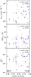 |
Fig. 4. Lyα observables (top panel: LLyα; middle panel: EWLyα; bottom panel: |

3.5. Relations between galaxy parameters, M⋆ and SFRHα, and global kinematical statistics
It is established that LAEs at high-z are preferentially low-mass (M⋆ ≲ 1010 M⊙) galaxies with star-formation rates on and slightly above the star-forming main sequence (SFR ∼ 10 M⊙ yr−1; e.g. Rhoads et al. 2014; Oyarzún et al. 2017; Kusakabe et al. 2018; Ouchi 2019; Pucha et al. 2022; Chávez Ortiz et al. 2023). Kinematically, the SFR is known to tightly correlate with the intrinsic velocity dispersion (e.g. Green et al. 2010, 2014; Law et al. 2022). The rotation velocity, vmax, directly traces mass. For rotating discs vshear ≤ vmax ⋅ sin(i) holds, where i is the inclination and vmax is the maximum value of the rotation curve; equality holds when the sampled velocity field reaches into the flat part of the rotation curve. Thus, before establishing and interpreting any relation between ionised gas kinematics and Lyα observables, we first need to investigate whether such correlations between physical galaxy parameters and galaxy kinematics exist in LARS+eLARS.
We begin by showing in Fig. 5 histograms of the distribution of M⋆ and SFRHα. These global quantities are measured from SED fitting to the HST images of the galaxies and the relevant details can be found in M23. The sample spans a M⋆ (SFRHα) range from 3.5 × 10⁹ M⊙ (0.15 M⊙yr−1) to 1.52 × 10¹¹ M⊙ (67 M⊙yr−1), with the mean and median being 3.2 × 10¹⁰ M⊙ (8.6 M⊙yr−1) and 2 × 10¹⁰ M⊙ (2.4 M⊙yr−1), respectively. The masses sample rather uniformly a decade above and half a decade below the characteristic stellar mass, M⋆*, of the stellar mass function of z ∼ 3 LAEs (M⋆* ≈ 4 × 10¹⁰ M⊙; Santos et al. 2021). LAE samples at high-z typically probe objects down to stellar masses of M⋆ ∼ 107 (Ouchi 2019, his Table 3.3), and the fraction of galaxies at lower masses than what is probed here is dominating in those samples. Nevertheless, here the different kinematic classes appear rather uniformly distributed over the masses and star-formation rates of our sample.
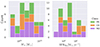 |
Fig. 5. Stacked histograms, colour-coded according to kinematical class (as in Fig. 2) of M⋆ (left panel) and SFRHα (right panel) from M23. |
In Fig. 6 we compare the relations between the kinematic parameters and M⋆ (left panel) or SFRHα (right panel). We also use Kendall’s rank correlation coefficient, τ, and the associated p-value, pτ, to reject the null-hypothesis of no correlation. The calculation of the uncertainty on τ and the assessment of the robustness of our correlation analyses against the error-bars of the parameters is determined via a Monte-Carlo simulation; further details are given in Appendix E. We recover both the σ0 vs. SFRHα relation and also the vshear vs. M⋆ relation at high significance (pτ < 10−4). The LARS+eLARS IFS sample thus shows the same correlations as larger samples that relate galaxy kinematics with M⋆ and SFR (e.g. Green et al. 2014; Moiseev et al. 2015; Barat et al. 2020; Law et al. 2022). Moreover, we also recover a relation between SFRHα and vshear. While this correlation shows a larger scatter and decreased |τ| value than the SFRHα vs.  relation it is also robust with respect to the error-bars. The correlation between SFRHα and vshear may be interpreted as the kinematical imprint of the star-formation main sequence. In Fig. 6 we can also appreciate that RDs have, unsurprisingly, overall higher vshear/σ0obs and higher vshear values than CKs and PRs.
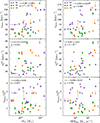 |
Fig. 6. Global kinematical measures vs. stellar mass (left panels) and star-formation rate (from Hα; right panels) for the LARS (squares) and eLARS galaxies (circles). The left-hand top-, middle-, and bottom panels show vshear vs. M⋆, σ vs. M⋆, and vshear/σ0obs vs. M⋆, respectively. The right-hand top-, middle-, and bottom panels, show vshear vs. SFRHα, |


Summarising, we find that the eLARS galaxies shows similar star-formation rates as found in high-z LAE samples, while their masses are found to be higher than the average masses such samples. Nevertheless, we recover the known trends between those parameters and galaxy kinematics of star-forming galaxies. We thus regard the eLARS sample as a representative probe for studying the relation between galaxy kinematics and Lyα observables, but being aware of potential caveats that arise from the bias towards higher masses (see Sect. 4).
3.6. Relations between global kinematical statistics and Lyα observables
When combining the observed trends between M⋆ or SFRHα and kinematical trends from Sect. 3.5 with the fact that LAEs are predominantly found amongst low-mass galaxies on and above the star-formation main sequence, it is expected that strong LAEs exhibit high velocity dispersions and small shearing amplitudes. This expectation is met by the LARS galaxies (H16) and was recently also reported for z ∼ 2 and z ∼ 3 galaxies by Foran et al. (2024). With the now enlarged sample and more carefully determined intrinsic velocity dispersions at hand (Appendix C) we can put these trends again to the test.
Using the canonical EWLyα ≥ 20 Å boundary to separate the sample into LAEs and non-LAEs, we find that the LAEs are characterised by a on average higher  than the non-LAEs:
  km s−1 vs.
  km s−1. Moreover, while the vshear values of LAEs and non-LAEs cover similar ranges (
 km s−1 vs.
  km s−1), LAEs tend to exhibit lower vshear/σ0obs ratios (
 ) than the non-LAEs (
 ). This indicates that the LAEs and non-LAEs are likely drawn from different underlying distributions in
  and vshear/σ0obs. This hypothesis is confirmed by a KS-test on the subsamples resulting from a split of LARS+eLARS at EWLyα = 20 Å with p-values of pKS < 10−3 for
  and pKS = 0.04 for vshear/σ0obs. However, in vshear the subsamples appear indistinguishable (pKS = 0.51). This result indicates that LAEs are more turbulent and show lower rotational support than non-LAEs.
We now investigate trends between the Lyα observables and the global kinematical characteristics. We do this graphically in Fig. 7, where we show a 3×3 scatter-plot matrix; the columns trace EWLyα,  , and LLyα on the abscissa (from left to right), whereas the rows trace vshear,
  , and vshear/σ0obs on the ordinate (from top to bottom). For each of the nine analysed relations we also compute Kendall’s τ and the corresponding pτ. The resulting τ and pτ values are provided in each subpanel of Fig. 7. We adopt the canonical pτ < 0.05 threshold for considering the scatter not being random. This corresponds to |τ|> 0.22 (|τ|> 0.21) for N = 38 (N = 42, for analysis involving only vshear; cf. Sect. 3.1) data points (Appendix E). We recover correlations for
  vs. EWLyα and
  vs. LLyα and we recover anti-correlations for vshear vs.
  and vshear/σ0obs vs.
  by adopting this threshold. All of these correlations are robust against perturbations due uncertainties on the involved measurements by the metric defined in Appendix E. Moreover, the data is suggestive of a anti-correlation between vshear/σ0obs and LLyα, although the obtained pτ is slightly above the canonical boundary of 0.05. We discuss the implications of our findings further in Sect. 4. For now we conclude that the data suggests that the kinematical state of a galaxy are in a causal relation to all three Lyα observables.
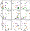 |
Fig. 7. Relations between ionised gas kinematics (vshear, |


As the correlation analysis tests the data for monotonicity, it fails to capture trends that cannot be described by a monotonic function. In this respect the panels for vshear vs. EWLyα or vshear/σ0obs vs. EWLyα in Fig. 7 appear noteworthy. Here we observe that low-EWLyα galaxies occupy almost the whole dynamical range sampled in vshear and vshear/σ0obs, whereas high-EWLyα galaxies are found predominantly at lower vshear and vshear/σ0obs values. More quantitatively, adopting the thresholds of EWLyα ≥ 20 Å for defining LAEs and vshear/σ0obs < 1.86 for defining dispersion dominated systems (cf. Sect. 3.3), we find that 9 out of 12 LAEs are dispersion dominated (75%). These 9 LAEs are also characterised by vshear < 100 km s−1. In this regard it appears also of interest to note that all galaxies classified as RDs in Sect. 3.2.1 do not qualify as dispersion dominated. If the trends found in the LARS+eLARS sample can be generalised, then we may suspect that LAEs are preferentially dispersion dominated systems with low velocity shearing and velocity fields that are, moreover, not commensurate with an unperturbed rotating disc.
4. Discussion
4.1. Assessing the importance of the kinematical parameters for the Lyα observables
Our analysis in Sect. 3.6 shows the potential importance of the global kinematical state of the ionised gas in a galaxy regarding its Lyα observables. We found significant correlations of  with EWLyα and LLyα, as well as the anti-correlations of vshear and vshear/σ0obs with fesc (Fig. 7). We reasoned that such relations are expected as they are the kinematical imprints of the fact that strong Lyα emitters are preferentially lower-mass systems with higher star-formation rates in comparison to weaker Lyα emitters or even absorbers. Of course, higher star-formation rates result in a larger amount of intrinsically produced Lyα photons, but we may further reason that feedback from star formation is creating an environment that facilitates easy escape of those photons. This may be especially the case in low-mass galaxies, where stellar winds and supernovae explosions can remove gas more efficiently because of their shallower gravitational potentials.
We recall that other galaxy characteristics are known to significantly affect the Lyα observability. In particular, the size and the dust content are of high relevance. Studies both at high-z and low-z show that LAEs are preferentially compact systems with only small amounts of dust (e.g. Guaita et al. 2010; Paulino-Afonso et al. 2018; Marchi et al. 2019; Paswan et al. 2022; Napolitano et al. 2023). The low dust content of LAEs is also reflected in their young ages and low metallicities. Moreover, the outflow kinematics and covering fraction of the scattering medium, probed by low-ionisation absorption lines in the rest-frame UV, are important; Lyα emitting galaxies are found to exhibit lower covering fractions and velocity offsets indicative of outflows (e.g. Wofford et al. 2013; Rivera-Thorsen et al. 2015; Trainor et al. 2015; Östlin et al. 2021; Reddy et al. 2022; Hayes 2023). Lastly, Lyα emitters exhibit higher degrees of ionisation and overall a harder UV radiation field (Trainor et al. 2016; Hayes et al. 2023). Clearly, Lyα production and the subsequent escape depend on a multitude of factors, and it is not at all intuitive which are the most important. Thus, we now want to quantify the importance of the global ionised gas kinematics regarding  , EWLyα, and LLyα (hereafter responses) relative to the other global observational and observationally inferred physical galaxy characteristics (hereafter parameters) of LARS+eLARS.
Assessing the relative parameter importance from a set of parameters with respect to a response is a difficult statistical problem. It is an area of active and controversial research and there exists no general agreed upon solution (see review by Grömping 2015). A main problem are intra-correlations between parameters, which lead to fundamental problems in defining the concept of importance. This hampers the robustness of the interpretation of heuristic approaches. Moreover, the more robust approaches implicitly assume that measurement errors are negligible, a situation unfortunately not encountered for the here considered responses and parameters. We thus opt for using rather simple metrics that were already applied in the context of understanding Lyα emission from galaxies (Runnholm et al. 2020, hereafter R20; Napolitano et al. 2023; Hayes 2023). Nevertheless, we also need to be aware of their shortcomings.
First, we use the absolute values of Kendall’s τ for each parameter on its own (Sect. 4.1.1). This so-called “marginal perspective” was recently used by Napolitano et al. (2023) alongside a Random Forrest classifier for identifying the important parameters that regulate EWLyα in high-z galaxies. The downside of the marginal perspective is that seemingly unimportant parameters may help each other in influencing the response variable (e.g. Guyon & Elisseeff 2003). For example, it may not be sufficient that a galaxy shows high O32 for having a large EWLyα, but the galaxy is also required to have a low Fcov – both parameters together may thus be of high-importance. Thus, we also need to analyse the problem from a “conditional perspective” (Grömping 2015). To this aim we first analyse all intra-parameter correlations in our sample before we follow R20 and Hayes et al. (2023) and adopt a procedure known as stepwise-regression in a multi-variable linear regression framework (Sect. 4.1.2).
As in R20 we define a purely observational parameter set and a physical parameter that is derived from the observational parameters. The observational parameter set consists of luminosities in the FUV, U, B, and I-band (expressed as luminosity densities LX, with X ∈ {FUV, U, B, I}), emission line luminosities of the lines Hα, Hβ, [O III] λ5007, [O II] λ3727 + λ3729, [N II] λ6584 (LY, with Y ∈ {Hα,Hβ,[O II],[O III][N II]}). The physical parameter set consists of stellar mass M⋆, the flux ratio between the [O III] and [O II] lines, O32 = F[O III],λ5007/(F[O II],λ3727 + [O II],λ3729) as proxy for the degree of ionisation, the nebular dust attenuation, E(B − V), the star-formation rate, SFRHα, the nebular oxygen abundance, 12 + log(O/H), the UV size sUV, as well as three parameters from low-ionisation absorption line measurements from HST/COS spectroscopy, namely the covering fraction Fcov, the line width, w90, and the velocity offset, v95, with respect to the systemic redshift determined from the nebular emission lines. All parameters are taken from R20 and M23; these publications detail the measurements of most of those parameters and we also refer to Rivera-Thorsen et al. (2015) and Hayes et al. (2023) for a description of the HST/COS based parameters. Both parameter sets consist of 9 parameters, which are again summarised in Table 1.
LARS+eLARS galaxy parameters against which the importance of vshear,  , and vsehar/σ0obs for regulating EWLyα,
  , and LLyα is assessed.
Lastly, in the following analyses we remove all six galaxies without detected Lyα emission from the statistical analyses presented below, since methods of the conditional perspective cannot deal with upper limits. As mentioned in Sect. 3.1, galaxies with double component Hα profiles are also not considered in our statistical analyses (i.e. we also have to remove additionally the three galaxies LARS 9, eLARS 7, and eLARS 24; LARS 13 has both double components and upper limits in the Lyα observables). Thus, the following analyses consider a sample of N = 33 galaxies.
4.1.1. Importance of kinematics: Marginal perspective
The marginal perspective regarding the importance of observational and physical parameters with respect to the responses EWLyα,  , and LLyα in LARS+eLARS is presented graphically in Fig. 8. We include the global kinematical statistics vshear,
  , and vshear/σ0obs in each of the two analysed parameter sets to asses their relative importance regarding the responses in comparison to the other parameters. In Fig. 8 we rank the parameters by the absolute values of Kendall’s τ. The rationale here is that |τ| is a direct measure of the frequency at which the change of a parameter leads to a parallel or anti-parallel change of the response. The higher the frequency of changes in the same direction, the higher the value of |τ|. Thus, an ordering of the parameters by |τ| can be interpreted as a ranking of their importance in influencing the response. As before, we deem a correlation significant if pτ < 0.05, which corresponds to |τ|> 0.239 (indicated by a vertical dashed line in Fig. 8) for N = 33. Moreover, the correlation is deemed robust if the inter-quartile range of τ’s from a Monte-Carlo simulation, that takes errors on the parameters and observables into account, does not overlap with this threshold (Appendix E).
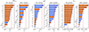 |
Fig. 8. Importance of observational and physical parameters for |


Focusing first on the response EWLyα we find that  dominates in importance over all parameters in the observational- and physical parameter sets. On the contrary, vshear is found to be least influential and, moreover, vshear/σ0obs appears also irrelevant. Formally, the emission line luminosities are ranked directly below
  , followed by the broad-band luminosity densities. However, here only the correlation with LHβ is statistically significant and robust. Lastly, consistent with the literature (e.g. Law et al. 2012; Paulino-Afonso et al. 2018), we find an anti-correlation between EWLyα and sUV. Taken together, these trends suggest that compact galaxies that are bright in the rest-frame optical emission lines, and which are characterised by a highly turbulent interstellar medium, are more likely to show higher EWLyα.
Next we focus on the response  . The kinematical parameters vshear and vshear/σ0obs, while not being highly ranked for EWLyα, emerge as highly influential parameters for fesc. Both anti-correlations dominate over all other observational parameters, albeit the correlation with vshear/σ0obs is not robust (Appendix E. Notably, except for L[O III] and L[N II], all observational parameters show even |τ|< 0.1 and appear thus individually completely irrelevant with respect to
  . This is also the case for
  . Regarding relations between physical parameters and
  we find that the anti-correlations with E(B − V) and Fcov are ranked higher than the anti-correlations with vshear. Moreover, the value of |τ| for vshear appears on par with the coefficient recovered for M⋆.
The high importance of  and simultaneous irrelevance of vshear or vshear/σ0 for regulating EWLyα appears noteworthy, given that the situation is reverse for
  . This situation is also evident in Fig. 7. Taken at face value, this is suggestive of different mechanisms regulating EWLyα and
  . This appears intriguing, because a tight linear relation between
  and EWLyα is found in our sample (M23), as well as in samples at higher redshifts (Sobral & Matthee 2019; Roy et al. 2023; Tang et al. 2023). However, in the following Sect. 4.1.2 we show that
  also emerges as an important parameter for regulating
  from the conditional perspective, but only when taken in concert with other parameters that are known to influence the Lyα radiative transfer.
Here we recover another intriguing discrepancy regarding the influence of individual parameters with respect to the responses  and EWLyα. Namely, we find that E(B − V) and M⋆ are not correlated with EWLyα, whereas both parameters anti-correlate with
  . Kinematically, the presence or absence of an anti-correlation between M⋆ and
  or EWLyα, respectively, is reflected in our sample by the different behaviour of both parameters with respect to vshear, which we just discussed. Moreover, this discrepancy does not vanish under the conditional perspective in Sect. 4.1.2 and it is appears also in contrast to some literature results (Marchi et al. 2019; Napolitano et al. 2023). Nevertheless, other studies also do not report monotonic relations between EWLyα and E(B − V) or M⋆ (Atek et al. 2014; Bolan et al. 2024).
Finally, we focus on the response LLyα. Here we find that all the other observational parameters are ranked above the kinematical parameters. However,  is ranked in second place amongst the physical parameters below SFRHα; vshear and vshear/σ0obs appear in the bottom half of the ranks and are thus not important in influencing LLyα. The strong relation between the emission line luminosities of Hβ and Hα for LLyα indicates that the production of intrinsic Lyα is a dominating cause in regulating the total Lyα photon output. This normalisation of Lyα luminosity by recombination rate is also reflected in the physical parameter set, where SFRHα (∝LHα) is ranked first.
As already mentioned in Sect. 4.1, we need to refrain from over-interpreting the rankings based on the marginal perspective for getting a grip on the physics that regulate the escape and observability of Lyα emission. For now we only conclude that our findings here are not inconsistent with the hypothesis that the global gas kinematics play a very important role in regulating the Lyα observables of a galaxy.
4.1.2. Importance of kinematics: Conditional perspective
In order to move away from the marginal perspective, we first analyse intra-parameter correlations in our parameter sets from Table 1. To this aim we use heat-map visualisations in Fig. 9. Using Kendall’s τ as a correlation measure Fig. 9 visualise the strength and directions of possible monotonic relations between all possible parameter combinations. The aim of this analysis is primarily to illustrate possible caveats when analysing only single parameter correlations with respect to the Lyα observables. We therefore also refrained from carrying out a robustness analysis on τ, instead we choose a more stringent p-value of pτ = 0.03 or, correspondingly, |τ|> 0.265 for N = 33 (Eq. (E.2)). Intra-parameter relations resulting in a smaller |τ| are crossed out in Fig. 9.
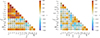 |
Fig. 9. Correlation matrix heat map visualisation (Kendall’s τ) for observational parameters (left panel) and physical parameters (right panel), including vshear, |


Considering the observational parameters in Fig. 9 (left panel) it becomes apparent that galaxies brighter in the continuum (irrespective of the band) are also almost always brighter in the rest-frame optical emission lines (τ ≳ 0.5, pτ ≲ 10−3) and also in the Lyα line. This “more is more” effect regarding LLyα might be specific to the here analysed sample that excludes Lyα absorbers. Regarding our kinematical parameters, only correlations between  and the emission lines, including Lyα, appear significant6, and references therein).
Focusing on the physical parameters in Fig. 9, we see that M⋆ shows the highest number of intra-correlations with other parameters; only lg(O/H) and E(B − V) are found not to be correlated with M⋆. Numerous other significant intra-correlations exist amongst the physical parameters. Amongst the kinematical parameters vshear/σ0obs correlates with vshear and anti-correlates with  . We also note that all Lyα observables correlate with each other. While some of the uncovered monotonic relations are certainly imprints of astrophysical scaling relations, other correlations or non-correlations might be specific to the sample at hand. We not discuss this further here, as this is not the main aim of our study. Of partilcular interest in our case, the high number of intra-correlations highlights the complex interdependence between the individual parameters in the observational and in the physical parameter sets. This complex network of relationships amongst the analysed parameters complicates the problem of assessing parameter importance, but it also highlights the need for a more sophisticated approach than just looking at parameter pairings.
We opt for a simple heuristic approach based on multi-variate regression,
 (3)
(3)
where the xi are the Np = 12 parameters from the observational- and physical parameter sets, respectively, including the kinematical parameters. The yi in Eq. (3) are the responses, i.e. here the Lyα observables, and the ci denote the coefficients maximising the coefficient of determination,
 (4)
(4)
where the fi are the predictions of the observable yi and ⟨yi⟩ is the mean over all yi. Formally, R2 encapsulates the variance explained by the empirical model of Eq. (3). If R2 ∼ 0, the linear relation in xi is not usable to describe and predict the yi, whereas for R2 ∼ 1 Eq. (3) is a nearly perfect empirical model.
In above framework we apply a forward and backward selection technique (also known as step-wise regression) to establish importance rankings for the parameters. Here we iteratively include (forward selection) or exclude (backward selection) parameters from Eq. (3), such that the included or excluded parameter leads to the largest increase or smallest decrease of R2, respectively. Moreover, this procedure requires that the parameters are standardised to a comparable scale. As in Hayes et al. (2023), here we use Z-score normalisation, that is, we subtract the mean over all values for each parameter and then we divide the mean shifted values by their standard deviation. Finally, we account for the statistical errors on the parameters and responses by performing NMC = 103 Monte-Carlo realisations of the above procedure. In each realisation we perturb both the response and the parameters according to their statistical uncertainties. This procedure provides us then with NMC ranks for each parameter xi under forward- and backward selection; we write for these j ranks rjFW(xi) and rjBW(xi), respectively, where j = 1, …, NMC.
We find that in almost all realisations the rankings obtained under forward selection are not completely consistent with the rankings obtained under backward selection. This so called “violation of anonymity” of the parameters regarding their positions in the regression is driven by the parameter intra-correlations (Fig. 9). It is a fundamental flaw of step-wise regression (Grömping 2015). This flaw also remains in bi-directional step-wise regression, where parameters are included and excluded in each iteration (Smith 2018). A potential alternative are more computational intensive methods related to game theory, which assign relative importance to a parameter based on all possible permutations that a parameter can have with all other parameters (Grömping 2015). However, given that we also require to include the measurement uncertainties via Monte Carlo simulations in our importance estimate, this approach is computationally expensive and will be the subject of future work. Here we instead opt for an ad hoc definition of a final ranking score. With
 (5)
(5)
we define the rank importance r(xi) of parameter xi as the average over all ranks obtained under forward and backward selection for a particular Monte Carlo realisation. The smaller r(xi), the more important is xi. The so obtained order of importance for the responses EWLyα,  , and LLyα are provided in Table 2.

Finally, following Hayes et al. (2023), we visualise in Fig. 10 the probability distributions of all ranks r(xi), p(r(xi)) by means of a Gaussian kernel-density estimator (kernel size 0.5). We highlight the four curves with the smallest r(xi) in Fig. 10, as these are formally the top ranked parameters according to Eq. (5). Moreover, we deem a high ranking of a parameter as robust if the p(r(xi)) curve for a given parameter peaks at a low r. Contrariwise, the ranking of a parameter is not considered as robust if the curve shows a flat distribution that encompasses a larger number of possible ranks. As can be seen from Fig. 10, and as we discuss below, for most of the parameters no clear order of importance can be established, even if a parameter is formally ranked high according to Eq. (5). However, for some parameters a clear picture emerges.
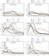 |
Fig. 10. Visualisation of the parameter importance for responses EWLyα (top panels), fescLyα (middle panels), and LLyα (bottom panels) from a conditional perspective using step-wise regression in a multivariate linear regression framework (see Sect. 4.1.2 for details). The panels on the left- and right-hand sides visualise the distribution of rankings p(r(xi)) for the parameters xi from the observational and physical parameter sets, respectively, where each set includes the kinematical parameters that have been derived in this work. Low values of r(xi) indicate a high importance of xi, whereas high values indicate a low importance. All but two of the curves were obtained using a kernel-density estimator (Gaussian kernel, width = 0.5) on the ranks from NMC = 103 Monte Carlo realisations. The exceptions are the |

The most notable and robust result from this statistical experiment is that σ0 is found as the most important parameter in determining EWLyα (top panels of Fig. 10). In fact, in almost all Monte-Carlo realisations  emerges as the top ranked parameter, both under forward and backward selection7. The dominating importance of σ0 in regulating EWLyα is thus found both from the marginal perspective (Sect. 4.1.1) and from the conditional perspective. We discuss this result in Sect. 4.2 below. Moreover, the distribution for the parameters ranked formally below
  do not show significant peaks. We thus regard the order of those parameters obtained by Eq. (5) not as robust indications of their relative importance with respect to EWLyα. The average R2 for all 12 parameters regarding the response EWLyα is 0.55 ± 0.04 and 0.50 ± 0.04 for the observational- and physical parameter set, respectively.
The distributions that we recover for the observational parameters with respect to  appear completely nondescript (centre left panel in Fig. 10). However, here a clearer picture emerges regarding the role of the physical parameter with respect to
  (centre right panel in Fig. 10). Here the four top ranked parameters – E(B − V), O32, Fcov, and σobs – are characterised by single peaked distributions in the left side of the diagram, whereas the remaining parameters show flattened out distributions towards the right side. For both parameter sets we recover an average R2 = 0.60 ± 0.05.
Attending the bottom panels of Fig. 10 we see that for LLyα the I-band luminosity arises as a top ranked observational parameter, with the other parameters not yielding conclusive rankings. Here R2 = 0.966 ± 0.003, but this high R2 is a result of the strong positive correlations of almost all parameters with LLyα. In the physical parameter set the top three ranked parameters – O32, M⋆, and Fcov – separate themselves distinctly from the remaining parameters. The R2 for the physical parameter set is 0.64 ± 0.05.
4.2. Astrophysical interpretation
Our analysis above leads us to the conclusion that  appears as a dominating parameter in regulating EWLyα when compared to other observational and physical parameters. This result is found both from the marginal – (Sect. 4.1.1) and from the conditional perspective (Sect. 4.1.2). A slightly different picture emerges regarding the role of
  with respect to
  . Here no direct correlation is found (Sect. 3.6 and Sect. 4.1.1), i.e.
  appears unimportant for
  when taken on its own, however it is found as an important parameter in regulating
  when considered in concert with other parameters (Sect. 4.1.2). These parameters are the neutral gas covering along the line of sight traced by Fcov, the ionisation state traced by O32, and the dust extinction traced by E(B − V). That these three other parameters are also expected and known to influence the escape of Lyα photons provides credibility to our method and result.
Unmistakably, Eq. (3) from Sect. 4.1.2 cannot replace an astrophysical model. This statistical method just helps to uncover trends in the data beyond the conventional two-parameter correlation analyses. The result from our statistical analysis requires us now to understand the dominant role of  for EWLyα and the role of
  in modulating
  .
.
4.2.1. The role of the age of the stellar population
The  values in our sample are all significantly above the expected combined velocity dispersions due to thermal and turbulent motions of the individual H II regions (
 km s−1 for T = 104 K). Therefore, the observed large values of
  are dominated by the turbulence of the cold and/or warm neutral medium in which the unresolved H II regions are embedded. The monotonic relation between SFR and σ0 (Sect. 3.5) thus indicates a causal connection between star-formation and turbulence of the interstellar medium.
There are competing scenarios regarding the main physical mechanism that are responsible for the SFR vs. σ0 relation. One the one hand, it is suggested that gravitational instabilities, which are required to form stars, may stir-up the interstellar medium and decay as turbulence (e.g. Krumholz & Burkert 2010). On the other hand, feedback from star-formation (i.e. stellar winds and especially supernovae) may act as the main source of energy driving this turbulence (e.g. Bacchini et al. 2020). Observational results are often used to argue in favour of latter scenario (Moiseev et al. 2015; Law et al. 2022), but there are also results that favour the former scenario (e.g. Krumholz & Burkhart 2016; Yu et al. 2021). Recent modelling by Ejdetjärn et al. (2022) indicates that the warm-ionised phase traced by Hα may actually also effectively couple to kinematic energy injected by feedback.
Adopting feedback as the driving force beyond σ0 as a working hypothesis we recall that for a simple stellar population the amount of energy injected by stellar winds and supernovae is related to the duration since the star-burst event (burst age, e.g. Leitherer et al. 1999). Furthermore, we recall that the intrinsic equivalent width, EWLyαint, is controlled by the ionising photon production efficiency, ξion, and both ξion and EWLyα are controlled by the burst age and metallicity (Charlot & Fall 1993; Schaerer 2003; Raiter et al. 2010; Inoue 2011). Thus, the evolutionary state of the stellar population is inherently linked to Lyα production, and given our working hypothesis and the results from Sect. 3.6 and Sect. 4.1.2, should also affect the escape of Lyα photons and modulate the observed equivalent width. Indeed, this idea finds support by the recent work of Hayes et al. (2023), who report a strong anti-correlation between EWLyα and burst age in their sample of 87 low-z galaxies observed with HST/COS. These authors also report an equally strong anti-correlation between burst age and  . If our hypothesis is true, then the effect that burst age has on EWLyα and
  should also be identifiable as an effect on
  .
.
In order to analyse the dependence of  , EWLyα, and
  on stellar age, we require estimates of the latter. The work by M23 provided age estimates for each Voronoi cell from the HST imaging data. We here use an average of those ages by weighing with the extinction corrected UV continuum. We note that our estimate differs from the age averages tabulated in M23, as these were only weighted by the extinction uncorrected UV continuum. As shown in Appendix F, where we also provide a table of the extinction corrected ages, for the majority of galaxies we now obtain significantly younger ages since the dust-uncorrected ages did not account for the very young populations enshrouded in dust.
We visualise the dependence of  , EWLyα, and
  on the so derived burst ages in Fig. 11. None of the three parameters are found to correlate with burst age. Hence, the anti-correlations between burst age and EWLyα or
  that were recovered in the sample of Hayes et al. (2023) are not found in our sample. However, a comparison with this sample is not on an equal footing. The crucial methodological difference is that Hayes et al. (2023) estimated stellar ages directly from fitting stellar templates to UV and optical spectra, whereas our ages are derived photometrically. Especially the UV spectra contain many age sensitive features (e.g. Chisholm et al. 2019). Nevertheless, the lack of a dirrect correlation between starburst age and
  may indicate that kinetic energy released from the stellar population and the conversion to turbulent energy follows more complex patterns.
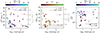 |
Fig. 11. Relations between |


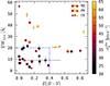 |
Fig. 12. Lyα equivalent width, EWLyα, vs. nebular extinction, E(B − V). Points are coloured according to |

To analyse this further we plot in Fig. 11 (upper panel) the evolution of mechanical luminosity (normalised to 1 M⊙) according to the STARBURST99 stellar population model (Leitherer et al. 1999) for a Z = 0.008 population (with a power law initial mass function of slope α = −2.35 and upper mass cut-off at 100 M⊙). To exemplify how EWLyαint depends on the burst-age we plot in the in the middle panel of Fig. 11 the EWLyαint evolution with time for a star-burst with Z = 0.008 Z⊙ according to the calculations by Inoue (2011). We also show the range of EWLyαint for similar types of low-Z populations with constant star formation from the calculations of Schaerer (2003). Considering the idealised star-burst, where all stars form instantaneously, initally winds from the highest mass stars (O stars) dominate the mechanical energy output. During these first few 106 years after the burst, the intrinsic Lyα equivalent widths are expected to be very high, with EWLyαint ∼ 300 Å at the typical metallicities (Z ∼ 10−2) of our sample. After ≈5 × 10⁶ years the injection of kinematic energy will increase substantially due to the most massive stars going supernova. The absence of ionising photons from these stars in otherwise very blue continua will lead to a gradual decrease of EWLyαint. At ≈107 years the O-stars are gone, the ionising luminosity drops by a factor of ∼100 compared to the initial phase of the burst, and the EWLyαint decreases even further. At this phase the now the injected kinetic energy stems only from stellar winds of lower mass stars.
Of course, the galaxies here consist of multiple clusters of different ages. Moreover, turbulent energy dissipates over varying timescales (∼10 − 100 Myr; e.g. Bacchini et al. 2020), so the link between mechanical luminosity or EWLyαint with burst age in Fig. 11 serves only as a schematic illustration. Still, in such a simple scenario, we would expect the lowest  values for the oldest population, but this is not what we observe. Also the trend for the EWs appears more nuanced. Except for one outlier, this plot is characterised by a zone of avoidance of old objects with high-EWs. Moreover, the highest EWs indeed appear at the youngest ages. Lastly, no discernible trend appears in the
  plot. We conclude that we do not recover the anticipated anti-correlation of burst-age on EWLyαint and
  , nor can we establish a causal relation between burst-age and
  .
.
4.2.2. Gas kinematics can shape dust geometry
We analyse in Fig. 12 the distribution of our sample in the EWLyα vs. E(B − V) plane. In this diagram we find a zone of avoidance: the five objects with the highest EWLyα measurements are found at low extinction (E(B − V) < 0.4), whereas the objects with lower EWLyα’s occupy the full range in E(B − V). The distribution of galaxies in the EWLyα vs. E(B − V) plane appears similar as in the compilation of low-z starbursts presented by Atek et al. (2014). We colour code the points in Fig. 12 by  to visualise the influence of this parameter on the observed EWLyα vs. E(B − V) distribution. While EWLyα is strongly correlated with
  (Sect. 3.6 and Sect. 4.1.1), we formally have to accept the null-hypothesis that
  and E(B − V) are not correlated (see also Fig. 9, numerically τ = 0.223 / p0 = 0.07). Still, in the E(B − V) vs. EWLyα plane it is apparent, how the corner of low extinction objects (0 ≤ E(B − V)≤0.4) with low Lyα equivalent widths (EWLyα ≤ 20 Å) appears to be dominated by galaxies with lower
  , whereas objects outside of this corner appear to be characterised by higher
  . These boundaries may appear somewhat arbitrary, but EWLyα ≥ 20 Å represents the canonical cut to define LAEs, while E(B − V) = 0.4 halves the E(B − V) range probed by our sample. We find that 18 objects with EWLyα ≤ 20 Å and 0 ≤ E(B − V)≤0.4 show a mean (median)
  of 32.8 km s−1 (31.2 km s−1), whereas the other 15 galaxies are characterised by a mean (median)
  of 50.3 km s−1 (51.2 km s−1). Thus, excluding objects in this low-σ0obs and low-E(B − V) region leaves us with objects that show simultaneously EWLyα > 20 Å and high velocity dispersions, but we also find galaxies with higher dust extinction that still show appreciable Lyα equivalent widths (EWLyα ≈ 20 Å) and, intriguingly, their intrinsic velocity dispersions are also high.
Next, we analyse in Fig. 13 the distribution of our sample in the  vs. EWLyα plane. There we also show the linear relation
  ∝ 4 × 10⁻³ EWLyα from M238. As in Fig. 12, we colour code the points by
  . We furthermore now highlight objects outside of the low-EWLyα – low-E(B − V) region defined in Fig. 12. We see that the dominant fraction of objects that are below the
  ∝ 4 × 10⁻³ EWLyα line are outside this E(B − V)≤0.4 and EWLyα ≤ 20 Å box of Fig. 12 (9 out of 12 objects). Thus, galaxies that have low
  but higher EWLyα are characterised by high
  .
.
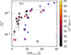 |
Fig. 13. Lyα escape fraction, |


Interestingly, almost all of the outliers below the fesc ∝ 4 × 10⁻³ EWLyα relation appear incompatible with extinction by a homogeneous dust screen. This can be appreciated in Fig. 14 where we plot the Lyα/Hα luminosity ratio against the Balmer decrement, Hα/Hβ, for our sample. In Fig. 14 we also indicate the expectation of Lyα/Hα as a function of Hα/Hβ for extinction by a homogeneous dust-screen in the absence of radiative transfer effects:
 (6)
(6)
Here
 (7)
(7)
and
 (8)
(8)
are the dust optical depths at λLyα and λHα, respectively; the definitions for (LLyα/LHα)int, k(λ), and E(B − V) were given in Sect. 2.4.
As discussed extensively in the literature, the intuition that the observed Lyα/Hα is always below the ratio given in Eq. (6) due to the loss of Lyα photons by radiative transfer effects proves often to be wrong (Scarlata et al. 2009; Atek et al. 2014; Hayes et al. 2014; Bridge et al. 2018; M23). As can be seen from Fig. 14, here we have 9 objects in our sample of 33 galaxies that are significantly above the pure dust attenuation expectation of Eq. (6). We also see in this figure that these 9 galaxies all are outside the EW ≤ 20 Å and E(B − V)≤0.4 box from Fig. 12. Moreover, 8 of those 9 galaxies are below the  ∝ 10−3EWLyα line from Fig. 13. Thus, galaxies that are not compatible with extinction by a homogeneous dust screen are characterised by high intrinsic velocity dispersions.
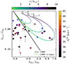 |
Fig. 14. Lyα/Hα ratio against the Hα/Hβ luminosity ratio for the in Sect. 4 analysed subsample of 33 galaxies as. there is no correlation between both quantities (τ = −0.09/pτ = 0.47). Symbols, colouring, and highlighting of the symbols is the same as in Fig. 13. The expectation of Lyα/Hα as a function of Hα/Hβ for a homogeneous dust-screen without radiative transfer effects in front of the line emission is shown as a solid line (Eq. (6)). The curves with a colour gradient indicate possible values for Lyα/Hα and Hα/Hβ for a clumpy dust screen, where on average NC = {3, 7, 9} clumps block the sight lines (Eq. (9)). These lines are drawn with a colour gradient that indicates the dust optical depth τC at 1216 Å of a single clump (colour bar at the top of the plot). |
Scarlata et al. (2009) point out that galaxies where the measured Lyα/Hα is higher than the expectation of Eq. (6), can be explained by obscuration by a system of dusty clumps, where on average NC clumps obscure the lines of sight. For this geometrical scenario Natta & Panagia (1984) derive the effective dust optical depth
 (9)
(9)
where τc(λ) is the dust optical depth of a single clump. In Fig. 14 we plot the curves from this scenario parameterised by τc(λLyα) for NC = {3, 5, 7}. Here we assume that the dust-extinction of the individual clumps obey also the Cardelli et al. (1989) law that was assumed for homogeneous screen. The notable feature of these curves is that they describe loops: With increasing dust optical depth the individual clumps start to significantly block emission over all involved lines and while the overall intensities decrease, with limτc → ∞τeff(λ) = NC, the ratio starts to become dominated by the sightlines that are not obscured by the dusty clumps. As evident from Fig. 14 all 9 galaxies above the expectation from Eq. (6) show Lyα/Hα ratios that are on or close to the loci associated with clumpy dust. Our analysis thus implies a connection between the small scale distribution of dust and ionised gas kinematics as traced by  .
.
4.2.3. The influence of turbulence on fescLyα
We close by discussing the anticipated effects of turbulence on Lyα radiative transfer in the very idealised set-up of a homogeneous static medium (e.g. Neufeld 1990; Verhamme et al. 2006; Laursen et al. 2009a). This idealised scattering medium is characterised by the density of neutral hydrogen, nH, or a corresponding neutral column, NH = nHs, along the path length s. Without turbulence the velocities of the atoms follow a Maxwellian distribution with the corresponding thermal velocity dispersion σtherm = 12.849 km s for a given temperature T4 in 104 K. Turbulent motions, characterised by a velocity dispersion σturb, broaden the velocity dispersion. In the framework of micro-turbulence this broadening is expressed by a convolution of the velocity distribution of the thermal motions with the velocity distribution of the turbulent motions (e.g. Verhamme et al. 2006; Smith et al. 2022). The intrinsic velocity dispersion is thus given by
  . Adopting Eq. (9) from Verhamme et al. (2006) we can express the monochromatic optical depth of this medium at the Lyα line centre as
![Mathematical equation: $$ \begin{aligned} \tau _{\lambda _{\mathrm {Ly}\alpha} } = 4.253 \times 10^{-13} \, \times \, \frac{N_\mathrm{H} \,[\mathrm{cm} ^{-2}]}{\sigma _0 \, [\mathrm{km} \,\mathrm{s} ^{-1}]} . \end{aligned} $$](/articles/aa/full_html/2025/01/aa51012-24/aa51012-24-eq156.gif) (10)
(10)
Hence, a highly turbulent medium will naturally become less opaque for resonant absorption of Lyα photons. The reduced optical depth will decrease the number of scatterings before a Lyα photon can escape the medium, and thereby reduce the probability that it will be absorbed by dust.
In fact, there exists an analytically derived approximate solution for  for the homogeneous static medium, if we assume a monochromatic Lyα source at the centre of a plane-parallel slab and if we assume that this medium is mixed with dust of optical depth τd, Lyα (Neufeld 1990). Following Verhamme et al. (2006) this solution can be written as
![Mathematical equation: $$ \begin{aligned} f_\mathrm{esc} ^{\mathrm {Ly}{\alpha}} \approx 1 \Bigg / \cosh \left( \frac{\sqrt{3}}{\pi ^{5/12} \zeta } \left[ \left( (a \tau _{\lambda _{\mathrm {Ly}\alpha} })^{1/3} \tau _{d,{\mathrm {Ly}{\alpha}} } \right)^{1/2} \right] \right) \; \text{.} \end{aligned} $$](/articles/aa/full_html/2025/01/aa51012-24/aa51012-24-eq158.gif) (11)
(11)
Here a = A21/4πΔνD, with A21 = 6.265 × 10⁸ s−1 being the Einstein coefficient of the Lyα transition and ΔνD = (σ0/c)×νLyα being the Doppler frequency broadening due to the thermal and turbulent motions (νLyα = 2.466 × 10¹⁵ Hz). Moreover, ζ in Eq. (11) is a fitting parameter that Neufeld (1990) derive to be ζ ≈ 0.525. Using Eq. (7) and Eq. (10) we can rewrite Eq. (11) as
![Mathematical equation: $$ \begin{aligned} f_\mathrm{esc} ^{\mathrm {Ly}{\alpha}} \approx 1 \Bigg / \cosh \left( 2.4 \times 10^{-2} \frac{( N_\mathrm{H} \,[\mathrm{cm} ^{-2}] )^{1/6} E(B-V)^{1/2}}{( \sigma _0 \, [\mathrm {km\,s} ^{-1}])^{2/6}} \right) \; \text{.} \end{aligned} $$](/articles/aa/full_html/2025/01/aa51012-24/aa51012-24-eq159.gif) (12)
(12)
This analysis shows that already in a very idealised set-up no simple monotonic relation between  and
and  is expected since additionally variations in neutral column and dust content will factor into the solution in a non-trivial manner. This result is in line with our finding that
  on its own does not affect
  (Sect. 4.1.1), but that it emerges as an important parameter in concert with E(B − V) and two other parameters (Fcov and O32, Sect. 4.1.2) that are related to the neutral column.
In Fig. 15 we show curves according to Eq. (12) in the  vs. σ0 parameter space for
  ,
,  , and E(B − V) values that are encountered in our sample. There we also plot the
  vs.
vs.  pairings of our sample colour coded by E(B − V). We see that the majority of our low-E(B − V) objects are commensurate with Eq. (12) for NH ∼ 1019 cm−2 and that high-E(B − V) objects would require lower neutral columns. However, most of these low-
 high-E(B − V) objects show Lyα/Hα ratios indicative of a clumpy dust distribution (Sect. 4.2.2).
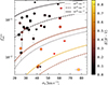 |
Fig. 15. Lyα escape fraction, |


We caution not to over overinterpret the comparison to the here presented analytic approximation, as Eq. (12) requires a highly idealised set-up. Our values on  trace the frequency distribution of the intrinsic Lyα radiation field, which is thus far from monochromatic, and the static plane-parallel slab oversimplifies the density and velocity distribution of the scattering medium encountered in reality. Moreover, Munirov & Kaurov (2023) recently highlighted the limited applicability of the micro-turbulence framework for Lyα radiative transfer. These authors show how the macroscopic nature of turbulence may significantly alter τLyα and thus also the number of scatterings and the spectral distribution Lyα photons emerging from a turbulent medium. This is because turbulence leads to zones of coherent velocities whose size- and velocity distributions are statistically described. Hence the simple convolution of the thermal- and turbulent velocity distributions used in the micro-turbulence framework may not be justified in reality. Munirov & Kaurov (2023) show especially that macroscopic turbulence can decrease the number of scatterings by orders of magnitude before Lyα photons escape the medium. While this underpins the importance of turbulence in regulating
  , quantitative inferences will require observational estimates of the characteristic scale lengths of the turbulent flows.
5. Conclusions
Here we present an analysis of the ionised gas kinematics obtained from all 42 galaxies that comprise the combined LARS+eLARS samples. The whole sample was observed in medium spectral resolution with the PMAS integral field unit at the Calar-Alto 3.5 m telescope. We constructed line-of-sight velocity fields and velocity-dispersion maps for each galaxy (Sect. 3.1) and present the newly obtained kinematic maps for the 28 eLARS galaxies (Fig. B.1). We combined this sample with the 14 galaxies that were analysed in H16. To date, this sample is the largest kinematical sample of galaxies that are also observed in Lyα emission and, thanks to the comprehensive HST imaging analyses of the sample presented in M23, now allows more robust statistical analyses regarding the possible trends found in H16. The reduced datacubes and the analysed velocity fields are released to the community with this publication. Our aim here is to check whether the Lyα observables EWLyα,  , and LLyα are affected by galaxy kinematics.
Our analysis of this sample revealed two null results. First, the Lyα observables are not affected by the morpho-kinematical nature of the velocity fields (Sect. 3.2.2). Second, the inclination of a system in our sample also does not affect the Lyα observables (Sect. 3.4). The first null result is new, and requires verification with larger samples at high redshift. The second result is in agreement with the null result found in photometric inclination estimates in high-z studies. Still, given the discrepancies between photometric and kinematic inclinations, verification with kinematical samples at high-z appears desirable.
We proceeded to quantify the global kinematical state of the galaxies via measurements of their intrinsic velocity dispersion,  (corrected for beam-smearing effects; Appendix C), and their projected maximum velocity amplitude, vshear (dubbed shearing velocity, Sect. 3.3). The gas kinematics of the sample are characterised by highly turbulent motions, with 30 km s−1 ≲ σ0obs ≲ 80 km s−1. Moreover, the majority of the shearing velocities in the sample are significantly below the values for disc galaxies. More than half of the sources of the sample (24 galaxies) show dispersion-dominated kinematics.
Our main result is that clear trends emerge between the kinematical measurements and the Lyα observables (Sect. 3.6). In particular, we find that EWLyα and LLyα correlate with  , whereas
  anti-correlates with vshear and vshear/σ0obs. Moreover, adopting the canonical criterion of EWLyα ≥ 20 Å to define a LAE, 75 % of the LAEs in our sample are dispersion-dominated systems; that is, they are characterised by vshear/σ0obs < 1.86. This result is in agreement with the recent study of high-z galaxies by Foran et al. (2024). We also find that
  strongly correlates with LLyα. However, this correlation is driven by the normalisation of LLyα with LHα in our sample. The trends uncovered here are commensurate with our initial hypothesis that the kinematics play an important role in regulating the Lyα observability of a galaxy.
We then tried to quantify the relative importance of the kinematical parameters with respect to other known observational and physical parameters of the galaxy sample. Our statistical analyses in Sect. 4.1.1 and Sect. 4.1.2 reveal that  emerges as a dominant variable in regulating EWLyα. We also find that
  is of significant importance regarding
  and LLyα. However, no clear trends regarding the importance of vshear or vshear/σ0obs emerged.
We note that the metrics used here to discuss the parameter importance are relatively simplistic. Moreover, our step-wise approach and also the marginal approach are actually criticised and disfavoured in the modern statistical literature (Grömping 2015; Smith 2018). Future analyses of the problem would benefit from more refined importance metrics, such as those reviewed by Grömping (2015). Adopting these methods is beyond the scope of the present analysis. Nevertheless, we suggest that the analysis of simple one-to-one correlations in particular might lead to erroneous conclusions or over-simplifications regarding the astrophysics of Lyα radiative transport.
While the empirical results are clear, we have not yet identified the dominating mechanism injecting turbulence and thereby regulating  . This complicates any interpretation of the fact that
  is found to be of utmost importance in regulating EWLyα. Motivated by results from stellar-population analysis, we discussed a simple scenario in which the age of the starburst simultaneously regulates
  ,
,  , and EWLyα. However, this scenario does not agree with our data.
That  is of dominating importance for regulating EWLyα while not being of similar importance for regulating
  deserves a closer look, especially because of the highly significant linear relationship between EWLyα and
  . In Sect. 4.2, we discuss the findings that galaxies that do not follow this linear relationship are often better described by a clumpy dust screen. However, those galaxies were also found to exhibit high
  . This suggests a connection between ionised gas kinematics and small-scale dust distribution.
Lastly, we discuss how, even in a highly idealised medium, a complicated interplay between NH, E(B − V), and σ0 is expected to influence  . We also highlight that the conventional treatment of turbulence as a microscopic effect may lead to underestimation of the actual quantitative influence of σ0 on
  . The results presented here suggest that further insight could be gained by investigating the trends we have uncovered in future analyses from a modelling and radiative transfer perspective, especially the role of turbulence in facilitating Lyα escape. Moreover, future spatially resolved kinematical studies of high-z galaxies with and without Lyα in emission could help us to understand whether or not our results are indeed applicable to the early Universe.
Data availability
The fully reduced PMAS cuboids are available at the CDS via anonymous ftp to cdsarc.cds.unistra.fr (130.79.128.5) or via https://cdsarc.cds.unistra.fr/viz-bin/cat/J/A+A/693/A252
Retrieved online from http://www.caha.es/pmas/PMAS_COOKBOOK/TABLES/pmas_gratings.html
At the relevant wavelengths in this work we have k(λHα) = 2.535, k(λHβ) = 3.793, and k(λLyα) = 10.862.
The morphology of eLARS 7 indicates that it is a merging system (see Fig. 4 in M23). Here the double component profiles occur in the region where the northern and the southern member of the interacting pair overlap. The situation is different in eLARS 24, where the morphology appears more disc-like (see Fig. 5 in M23). Here the double component profiles appear most pronounced towards south-western part, perhaps indicating an infalling star-forming satellite galaxy. Furthermore, according to the catalogue of Tempel et al. (2017), eLARS 24 resides in a group environment where frequent mergers would be expected, and an H I envelope that encompasses the nearest neighbour 30″ towards the south west confirms the merger hypothesis (Le Reste et al., in prep.).
Throughout we measure correlations with the generalised Kendall-τ correlation coefficient according to Isobe et al. (1986) as this formalism allows us to treat upper limits sensibly in the analysis. Moreover, following Curran (2014) we use a Monte-Carlo procedure for the calculation of the error on τ. More details are given in Appendix E.
The relation between  (and also σtot) and optical emission lines in star-forming galaxies is well known (Terlevich & Melnick 1981), albeit its physical origins are debated. Nevertheless, these trends have been suggested as an alternative cosmological standard candle (e.g. González-Morán et al. 2019).
For this reason, we have to visualise the probability density p(r(σ0obs)) in Fig. 10 as a histogram, since the kernel density estimator would produce a highly peaked narrow curve, whose visualisation would render the other curves indistinguishable.
The slope from Melinder et al. (2023) is identical to the slope of the z ∈ {0, 0.3} sample from Sobral & Matthee (2019), but slightly shallower than then the slope found by these authors at higher redshifts ( ∝ 5 × 10⁻³ EWLyα).
Version 2.6.4 obtained from https://p3d.sourceforge.io/.
The website https://www.anisotropela.dk/work/lars/hst2pmas documents this effort.
This problem is illustrated by the application of a rotating disc model to the complex velocity field of the star-burst SBS 0335-052E by Isobe et al. (2023). The recovered kinematical parameters and, especially, the kinematical position angle differ significantly compared to a modified disc model that Moiseev et al. (2010) used for this galaxy. Their model accounts for a kinematical disturbance caused by an expanding super-bubble. Such modified models, however, need to be defined on an object by object basis (see especially Sardaneta et al. 2020 for an idea of a model for eLARS01), which is not practical for a statistical analysis.
Both the computation of the generalised Kendall’s τ and the Monte-Carlo simulation were implemented in python and are available at https://github.com/Knusper/kendall.
Evaluating the exact distribution of |τ| under the null hypothesis, which cannot be expressed as a simple formula, results in marginally different thresholds, |τ|> {0.213, 0.223, 0.242, 0.390}, but without any implication for our results.
Acknowledgments
Based on observations collected at the Centro Astronómico Hispano-Alemán (CAHA) at Calar Alto, operated jointly by Junta de Andalucía and Consejo Superior de Investigaciones Científicas (IAA-CSIC). The authors acknowledge financial support by the Centre National D’Etudes Spatiales (CNES). We acknowledge the use of the following software: ds9 (Joye & Mandel 2003), QFitsView (Ott 2012), Astropy (Astropy Collaboration 2022), Numpy (Harris et al. 2020), SciPy (Virtanen et al. 2020), matplotlib Hunter (2007), seaborn (Waskom 2021), cmasher (van der Velden 2020), GalPak3D (Bouché et al. 2015), dust_extinction (Gordon 2024), and p3d (Sandin et al. 2010). MH is fellow of the Knut & Alice Wallenberg Foundation. AS acknowledges the support by Jörg Main and the hospitality at Institute for Theoretical Physics 1 (Stuttgart University) to carry out this research. AS’s contribution to this project was partly made possible by funding from the Carl-Zeiss-Stiftung. We thank especially Daniel Kunth for organising meetings at Institut Astrophysique de Paris and for continuous support with the project. ECH and AS acknowledge travel funds provided by the IAP for attending these meetings. We thank N. Bouché for support regarding the use of GalPak3D. We thank Rikke Saust as well as the motivated staff at Calar-Alto observatory for help with the preparation and execution of the visitor mode observations. ECH acknowledges the generous hospitality of Leiden University for carrying out parts of this research. ECH acknowledges funding of an internship for AS within the DAAD RISE scheme. ECH dedicates this work in loving memory to a cat named Pixel.
References
- Alonso-Herrero, A., García-Marín, M., Monreal-Ibero, A., et al. 2009, A&A, 506, 1541 [NASA ADS] [CrossRef] [EDP Sciences] [Google Scholar]
- Arrabal Haro, P., Dickinson, M., Finkelstein, S. L., et al. 2023, Nature, 622, 707 [NASA ADS] [CrossRef] [Google Scholar]
- Astropy Collaboration (Price-Whelan, A. M., et al.) 2022, ApJ, 935, 167 [NASA ADS] [CrossRef] [Google Scholar]
- Atek, H., Kunth, D., Schaerer, D., et al. 2014, A&A, 561, A89 [NASA ADS] [CrossRef] [EDP Sciences] [Google Scholar]
- Bacchini, C., Fraternali, F., Iorio, G., et al. 2020, A&A, 641, A70 [NASA ADS] [CrossRef] [EDP Sciences] [Google Scholar]
- Barat, D., D’Eugenio, F., Colless, M., et al. 2020, MNRAS, 498, 5885 [NASA ADS] [CrossRef] [Google Scholar]
- Behrens, C., & Braun, H. 2014, A&A, 572, A74 [NASA ADS] [CrossRef] [EDP Sciences] [Google Scholar]
- Bernal, J. L., & Kovetz, E. D. 2022, A&ARv, 30, 5 [NASA ADS] [CrossRef] [Google Scholar]
- Bik, A., Östlin, G., Hayes, M., Melinder, J., & Menacho, V. 2022, A&A, 666, A161 [NASA ADS] [CrossRef] [EDP Sciences] [Google Scholar]
- Blaizot, J., Garel, T., Verhamme, A., et al. 2023, MNRAS, 523, 3749 [NASA ADS] [CrossRef] [Google Scholar]
- Blanc, G. A., Adams, J. J., Gebhardt, K., et al. 2011, ApJ, 736, 31 [CrossRef] [Google Scholar]
- Bolan, P., Bradăc, M., Lemaux, B. C., et al. 2024, MNRAS, 531, 2998 [Google Scholar]
- Bouché, N., Carfantan, H., Schroetter, I., Michel-Dansac, L., & Contini, T. 2015, AJ, 150, 92 [Google Scholar]
- Boyett, K., Trenti, M., Leethochawalit, N., et al. 2024, Nat. Astron. [arXiv:2303.00306] [Google Scholar]
- Bridge, J. S., Hayes, M., Melinder, J., et al. 2018, ApJ, 852, 9 [Google Scholar]
- Bunker, A. J., Saxena, A., Cameron, A. J., et al. 2023, A&A, 677, A88 [NASA ADS] [CrossRef] [EDP Sciences] [Google Scholar]
- Cannon, J. M., Skillman, E. D., Kunth, D., et al. 2004, ApJ, 608, 768 [NASA ADS] [CrossRef] [Google Scholar]
- Cardelli, J. A., Clayton, G. C., & Mathis, J. S. 1989, ApJ, 345, 245 [Google Scholar]
- Charlot, S., & Fall, S. M. 1993, ApJ, 415, 580 [Google Scholar]
- Chávez Ortiz, Ó. A., Finkelstein, S. L., Davis, D., et al. 2023, ApJ, 952, 110 [NASA ADS] [CrossRef] [Google Scholar]
- Chisholm, J., Rigby, J. R., Bayliss, M., et al. 2019, ApJ, 882, 182 [Google Scholar]
- Choudhury, T. R. 2022, Gen. Rel. Grav., 54, 102 [NASA ADS] [CrossRef] [Google Scholar]
- Curran, P. A. 2014, ArXiv e-prints [arXiv:1411.3816] [Google Scholar]
- Davies, R., Förster Schreiber, N. M., Cresci, G., et al. 2011, ApJ, 741, 69 [NASA ADS] [CrossRef] [Google Scholar]
- Dayal, P., & Libeskind, N. I. 2012, MNRAS, 419, L9 [NASA ADS] [CrossRef] [Google Scholar]
- Dijkstra, M. 2014, PASA, 31, 40 [NASA ADS] [CrossRef] [Google Scholar]
- Dijkstra, M. 2019, Saas-Fee Adv. Course, 46, 1 [NASA ADS] [CrossRef] [Google Scholar]
- Dijkstra, M., & Wyithe, J. S. B. 2012, MNRAS, 419, 3181 [NASA ADS] [CrossRef] [Google Scholar]
- Ejdetjärn, T., Agertz, O., Östlin, G., Renaud, F., & Romeo, A. B. 2022, MNRAS, 514, 480 [CrossRef] [Google Scholar]
- Epinat, B., Amram, P., & Marcelin, M. 2008, MNRAS, 390, 466 [NASA ADS] [Google Scholar]
- Epinat, B., Amram, P., Balkowski, C., & Marcelin, M. 2010, MNRAS, 401, 2113 [Google Scholar]
- Ferruit, P. 2010, in 3D Spectroscopy in Astronomy, eds. E. Mediavilla, S. Arribas, M. Roth, J. Cepa-Nogue, & F. Sanchez (Cambridge: Cambridge University Press), 126 [CrossRef] [Google Scholar]
- Finkelstein, S. L., Rhoads, J. E., Malhotra, S., & Grogin, N. 2009, ApJ, 691, 465 [NASA ADS] [CrossRef] [Google Scholar]
- Foran, G., Cooke, J., Wisnioski, E., Reddy, N., & Steidel, C. 2024, PASA, 41, e005 [CrossRef] [Google Scholar]
- Forero-Romero, J. E., Yepes, G., Gottlöber, S., et al. 2011, MNRAS, 415, 3666 [NASA ADS] [CrossRef] [Google Scholar]
- Förster Schreiber, N. M., & Wuyts, S. 2020, ARA&A, 58, 661 [Google Scholar]
- Fruchter, A. S., & Hook, R. N. 2002, PASP, 114, 144 [NASA ADS] [CrossRef] [Google Scholar]
- Garel, T., Blaizot, J., Guiderdoni, B., et al. 2015, MNRAS, 450, 1279 [Google Scholar]
- Garel, T., Guiderdoni, B., & Blaizot, J. 2016, MNRAS, 455, 3436 [NASA ADS] [CrossRef] [Google Scholar]
- Gebhardt, K., Mentuch Cooper, E., Ciardullo, R., et al. 2021, ApJ, 923, 217 [NASA ADS] [CrossRef] [Google Scholar]
- Giavalisco, M., Koratkar, A., & Calzetti, D. 1996, ApJ, 466, 831 [NASA ADS] [CrossRef] [Google Scholar]
- Glazebrook, K. 2013, PASA, 30, 56 [CrossRef] [Google Scholar]
- Gnerucci, A., Marconi, A., Cresci, G., et al. 2011, A&A, 528, A88 [NASA ADS] [CrossRef] [EDP Sciences] [Google Scholar]
- González-Morán, A. L., Chávez, R., Terlevich, R., et al. 2019, MNRAS, 487, 4669 [CrossRef] [Google Scholar]
- Gordon, K. 2024, dust_extinction, https://doi.org/10.5281/zenodo.11235336 [Google Scholar]
- Graham, A. W., & Driver, S. P. 2005, PASA, 22, 118 [NASA ADS] [CrossRef] [Google Scholar]
- Green, A. W., Glazebrook, K., McGregor, P. J., et al. 2010, Nature, 467, 684 [NASA ADS] [CrossRef] [Google Scholar]
- Green, A. W., Glazebrook, K., McGregor, P. J., et al. 2014, MNRAS, 437, 1070 [Google Scholar]
- Greisen, E. W., & Calabretta, M. R. 2002, A&A, 395, 1061 [NASA ADS] [CrossRef] [EDP Sciences] [Google Scholar]
- Grömping, U. 2015, WIREs. Comput. Stat., 7, 137 [Google Scholar]
- Gronke, M., Ocvirk, P., Mason, C., et al. 2021, MNRAS, 508, 3697 [NASA ADS] [CrossRef] [Google Scholar]
- Gronwall, C., Bond, N. A., Ciardullo, R., et al. 2011, ApJ, 743, 9 [NASA ADS] [CrossRef] [Google Scholar]
- Guaita, L., Gawiser, E., Padilla, N., et al. 2010, ApJ, 714, 255 [NASA ADS] [CrossRef] [Google Scholar]
- Gurung-López, S., Orsi, Á. A., Bonoli, S., Baugh, C. M., & Lacey, C. G. 2019, MNRAS, 486, 1882 [Google Scholar]
- Guyon, I., & Elisseeff, A. 2003, J. Mach. Learn. Res., 3, 1157 [Google Scholar]
- Hagen, A., Zeimann, G. R., Behrens, C., et al. 2016, ApJ, 817, 79 [CrossRef] [Google Scholar]
- Harris, C. R., Millman, K. J., van der Walt, S. J., et al. 2020, Nature, 585, 357 [NASA ADS] [CrossRef] [Google Scholar]
- Hathi, N. P., Le Fèvre, O., Ilbert, O., et al. 2016, A&A, 588, A26 [NASA ADS] [CrossRef] [EDP Sciences] [Google Scholar]
- Hayes, M. 2015, PASA, 32, 27 [NASA ADS] [CrossRef] [Google Scholar]
- Hayes, M. J. 2023, MNRAS, 519, L26 [Google Scholar]
- Hayes, M., Östlin, G., Mas-Hesse, J. M., & Kunth, D. 2009, AJ, 138, 911 [NASA ADS] [CrossRef] [Google Scholar]
- Hayes, M., Scarlata, C., & Siana, B. 2011, Nature, 476, 304 [NASA ADS] [CrossRef] [Google Scholar]
- Hayes, M., Östlin, G., Duval, F., et al. 2014, ApJ, 782, 6 [NASA ADS] [CrossRef] [Google Scholar]
- Hayes, M. J., Runnholm, A., Scarlata, C., Gronke, M., & Rivera-Thorsen, T. E. 2023, MNRAS, 520, 5903 [NASA ADS] [CrossRef] [Google Scholar]
- Heintz, K. E., Watson, D., Brammer, G., et al. 2024, Science, 384, 890 [NASA ADS] [CrossRef] [Google Scholar]
- Henry, A., Scarlata, C., Martin, C. L., & Erb, D. 2015, ApJ, 809, 19 [Google Scholar]
- Herenz, E. C., Gruyters, P., Orlitova, I., et al. 2015, VizieR Online Data Catalog, J/A+A/587/A78. [Google Scholar]
- Herenz, E. C., Gruyters, P., Orlitova, I., et al. 2016, A&A, 587, A78 [NASA ADS] [CrossRef] [EDP Sciences] [Google Scholar]
- Herenz, E. C., Wisotzki, L., Saust, R., et al. 2019, A&A, 621, A107 [NASA ADS] [CrossRef] [EDP Sciences] [Google Scholar]
- Horne, K. 1986, PASP, 98, 609 [Google Scholar]
- Hunter, J. D. 2007, Comput. Sci. Eng., 9, 90 [NASA ADS] [CrossRef] [Google Scholar]
- Inoue, A. K. 2011, MNRAS, 415, 2920 [NASA ADS] [CrossRef] [Google Scholar]
- Isobe, T., Feigelson, E. D., & Nelson, P. I. 1986, ApJ, 306, 490 [Google Scholar]
- Isobe, Y., Ouchi, M., Nakajima, K., et al. 2023, ApJ, 951, 102 [NASA ADS] [CrossRef] [Google Scholar]
- Joye, W. A., & Mandel, E. 2003, ASP Conf. Ser., 295, 489 [Google Scholar]
- Kauffmann, G., Heckman, T. M., Tremonti, C., et al. 2003, MNRAS, 346, 1055 [Google Scholar]
- Keel, W. C. 2005, AJ, 129, 1863 [NASA ADS] [CrossRef] [Google Scholar]
- Kewley, L. J., Dopita, M. A., Sutherland, R. S., Heisler, C. A., & Trevena, J. 2001, ApJ, 556, 121 [Google Scholar]
- Konno, A., Ouchi, M., Shibuya, T., et al. 2018, PASJ, 70, S16 [Google Scholar]
- Krajnović, D., Cappellari, M., de Zeeuw, P. T., & Copin, Y. 2006, MNRAS, 366, 787 [Google Scholar]
- Kramarenko, I. G., Kerutt, J., Verhamme, A., et al. 2024, MNRAS, 527, 9853 [Google Scholar]
- Krumholz, M., & Burkert, A. 2010, ApJ, 724, 895 [NASA ADS] [CrossRef] [Google Scholar]
- Krumholz, M. R., & Burkhart, B. 2016, MNRAS, 458, 1671 [NASA ADS] [CrossRef] [Google Scholar]
- Kunth, D., Mas-Hesse, J. M., Terlevich, E., et al. 1998, A&A, 334, 11 [NASA ADS] [Google Scholar]
- Kusakabe, H., Shimasaku, K., Ouchi, M., et al. 2018, PASJ, 70, 4 [Google Scholar]
- Landman, D. A., Roussel-Dupre, R., & Tanigawa, G. 1982, ApJ, 261, 732 [CrossRef] [Google Scholar]
- Lao, B.-X., & Smith, A. 2020, MNRAS, 497, 3925 [CrossRef] [Google Scholar]
- Laursen, P., & Sommer-Larsen, J. 2007, ApJ, 657, L69 [NASA ADS] [CrossRef] [Google Scholar]
- Laursen, P., Razoumov, A. O., & Sommer-Larsen, J. 2009a, ApJ, 696, 853 [NASA ADS] [CrossRef] [Google Scholar]
- Laursen, P., Sommer-Larsen, J., & Andersen, A. C. 2009b, ApJ, 704, 1640 [Google Scholar]
- Laursen, P., Sommer-Larsen, J., Milvang-Jensen, B., Fynbo, J. P. U., & Razoumov, A. O. 2019, A&A, 627, A84 [NASA ADS] [CrossRef] [EDP Sciences] [Google Scholar]
- Law, D. R., Steidel, C. C., Shapley, A. E., et al. 2012, ApJ, 759, 29 [NASA ADS] [CrossRef] [Google Scholar]
- Law, D. R., Belfiore, F., Bershady, M. A., et al. 2022, ApJ, 928, 58 [CrossRef] [Google Scholar]
- Le Reste, A., Hayes, M., Cannon, J. M., et al. 2022, ApJ, 934, 69 [NASA ADS] [CrossRef] [Google Scholar]
- Le Reste, A., Cannon, J. M., Hayes, M. J., et al. 2024, MNRAS, 528, 757 [NASA ADS] [CrossRef] [Google Scholar]
- Leitherer, C., Schaerer, D., Goldader, J. D., et al. 1999, ApJS, 123, 3 [Google Scholar]
- Lenz, D. D., & Ayres, T. R. 1992, PASP, 104, 1104 [NASA ADS] [CrossRef] [Google Scholar]
- Li, Z., Steidel, C. C., Gronke, M., Chen, Y., & Matsuda, Y. 2022, MNRAS, 513, 3414 [NASA ADS] [CrossRef] [Google Scholar]
- Lin, X., Cai, Z., Wu, Y., et al. 2024, ApJS, 272, 33 [NASA ADS] [CrossRef] [Google Scholar]
- Liu, W., & Jiang, L. 2023, ApJ, 958, 187 [NASA ADS] [CrossRef] [Google Scholar]
- Lujan Niemeyer, M., Bernal, J. L., & Komatsu, E. 2023, ApJ, 958, 4 [NASA ADS] [CrossRef] [Google Scholar]
- Malhotra, S., Rhoads, J. E., Finkelstein, S. L., et al. 2012, ApJ, 750, L36 [NASA ADS] [CrossRef] [Google Scholar]
- Marchi, F., Pentericci, L., Guaita, L., et al. 2019, A&A, 631, A19 [NASA ADS] [CrossRef] [EDP Sciences] [Google Scholar]
- Maseda, M. V., Bacon, R., Lam, D., et al. 2020, MNRAS, 493, 5120 [Google Scholar]
- Matthee, J., Sobral, D., Santos, S., et al. 2015, MNRAS, 451, 400 [Google Scholar]
- Matthee, J., Sobral, D., Hayes, M., et al. 2021, MNRAS, 505, 1382 [NASA ADS] [CrossRef] [Google Scholar]
- McCarron, A. P., Finkelstein, S. L., Chavez Ortiz, O. A., et al. 2022, ApJ, 936, 131 [NASA ADS] [CrossRef] [Google Scholar]
- Melinder, J., Östlin, G., Hayes, M., et al. 2023, ApJS, 266, 15 [NASA ADS] [CrossRef] [Google Scholar]
- Mentuch Cooper, E., Gebhardt, K., Davis, D., et al. 2023, ApJ, 943, 177 [NASA ADS] [CrossRef] [Google Scholar]
- Moiseev, A. V., Pustilnik, S. A., & Kniazev, A. Y. 2010, MNRAS, 405, 2453 [NASA ADS] [Google Scholar]
- Moiseev, A. V., Tikhonov, A. V., & Klypin, A. 2015, MNRAS, 449, 3568 [NASA ADS] [CrossRef] [Google Scholar]
- Munirov, V. R., & Kaurov, A. A. 2023, MNRAS, 522, 2747 [NASA ADS] [CrossRef] [Google Scholar]
- Nakajima, K., Ellis, R. S., Iwata, I., et al. 2016, ApJ, 831, L9 [Google Scholar]
- Nakajima, K., Fletcher, T., Ellis, R. S., Robertson, B. E., & Iwata, I. 2018, MNRAS, 477, 2098 [NASA ADS] [CrossRef] [Google Scholar]
- Nakane, M., Ouchi, M., Nakajima, K., et al. 2024, ApJ, 967, 28 [NASA ADS] [CrossRef] [Google Scholar]
- Napolitano, L., Pentericci, L., Calabrò, A., et al. 2023, A&A, 677, A138 [NASA ADS] [CrossRef] [EDP Sciences] [Google Scholar]
- Natta, A., & Panagia, N. 1984, ApJ, 287, 228 [NASA ADS] [CrossRef] [Google Scholar]
- Neufeld, D. A. 1990, ApJ, 350, 216 [NASA ADS] [CrossRef] [Google Scholar]
- Ning, Y., Jiang, L., Zheng, Z.-Y., & Wu, J. 2022, ApJ, 926, 230 [NASA ADS] [CrossRef] [Google Scholar]
- Östlin, G., Hayes, M., Duval, F., et al. 2014, ApJ, 797, 11 [CrossRef] [Google Scholar]
- Östlin, G., Rivera-Thorsen, T. E., Menacho, V., et al. 2021, ApJ, 912, 155 [CrossRef] [Google Scholar]
- Ott, T. 2012, QFitsView: FITS file viewer, Astrophysics Source Code Library [record ascl:1210.019] [Google Scholar]
- Ouchi, M. 2019, Saas-Fee Adv. Course, 46, 189 [NASA ADS] [CrossRef] [Google Scholar]
- Ouchi, M., Shimasaku, K., Akiyama, M., et al. 2008, ApJS, 176, 301 [Google Scholar]
- Ouchi, M., Shimasaku, K., Furusawa, H., et al. 2010, ApJ, 723, 869 [Google Scholar]
- Ouchi, M., Ono, Y., & Shibuya, T. 2020, ARA&A, 58, 617 [Google Scholar]
- Oyarzún, G. A., Blanc, G. A., González, V., et al. 2016, ApJ, 821, L14 [CrossRef] [Google Scholar]
- Oyarzún, G. A., Blanc, G. A., González, V., Mateo, M., & Bailey, J. I., 2017, ApJ, 843, 133 [CrossRef] [Google Scholar]
- Pardy, S. A., Cannon, J. M., Östlin, G., et al. 2014, ApJ, 794, 101 [NASA ADS] [CrossRef] [Google Scholar]
- Partridge, R. B., & Peebles, P. J. E. 1967, ApJ, 147, 868 [Google Scholar]
- Paswan, A., Saha, K., Leitherer, C., & Schaerer, D. 2022, ApJ, 924, 47 [NASA ADS] [CrossRef] [Google Scholar]
- Paulino-Afonso, A., Sobral, D., Ribeiro, B., et al. 2018, MNRAS, 476, 5479 [NASA ADS] [CrossRef] [Google Scholar]
- Pucha, R., Reddy, N. A., Dey, A., et al. 2022, AJ, 164, 159 [NASA ADS] [CrossRef] [Google Scholar]
- Puka, L. 2011, Kendall’s Tau (Springer Berlin Heidelberg), 713 [Google Scholar]
- Purkayastha, S., Kanekar, N., Chengalur, J. N., et al. 2022, ApJ, 933, L11 [NASA ADS] [CrossRef] [Google Scholar]
- Puschnig, J., Hayes, M., Östlin, G., et al. 2020, A&A, 644, A10 [NASA ADS] [CrossRef] [EDP Sciences] [Google Scholar]
- Raiter, A., Schaerer, D., & Fosbury, R. A. E. 2010, A&A, 523, A64 [NASA ADS] [CrossRef] [EDP Sciences] [Google Scholar]
- Rasekh, A., Melinder, J., Östlin, G., et al. 2022, A&A, 662, A64 [NASA ADS] [CrossRef] [EDP Sciences] [Google Scholar]
- Reddy, N. A., Topping, M. W., Shapley, A. E., et al. 2022, ApJ, 926, 31 [NASA ADS] [CrossRef] [Google Scholar]
- Remolina-Gutiérrez, M. C., & Forero-Romero, J. E. 2019, MNRAS, 482, 4553 [Google Scholar]
- Rhoads, J. E., Malhotra, S., Richardson, M. L. A., et al. 2014, ApJ, 780, 20 [Google Scholar]
- Rivera-Thorsen, T. E., Hayes, M., Östlin, G., et al. 2015, ApJ, 805, 14 [Google Scholar]
- Robertson, J. G. 2017, PASA, 34, e035a [NASA ADS] [CrossRef] [Google Scholar]
- Robitaille, T., Deil, C., & Ginsburg, A. 2020, reproject: Python-based astronomical image reprojection, Astrophysics Source Code Library [record ascl:2011.023] [Google Scholar]
- Roth, M. M., Kelz, A., Fechner, T., et al. 2005, PASP, 117, 620 [Google Scholar]
- Roy, N., Henry, A., Treu, T., et al. 2023, ApJ, 952, L14 [NASA ADS] [CrossRef] [Google Scholar]
- Runnholm, A., Hayes, M., Melinder, J., et al. 2020, ApJ, 892, 48 [NASA ADS] [CrossRef] [Google Scholar]
- Sandin, C., Becker, T., Roth, M. M., et al. 2010, A&A, 515, A35 [NASA ADS] [CrossRef] [EDP Sciences] [Google Scholar]
- Sandin, C., Weilbacher, P., Tabataba-Vakili, F., Kamann, S., & Streicher, O. 2012, Proc. SPIE, 8451, 84510F [NASA ADS] [CrossRef] [Google Scholar]
- Santos, S., Sobral, D., & Matthee, J. 2016, MNRAS, 463, 1678 [Google Scholar]
- Santos, S., Sobral, D., Butterworth, J., et al. 2021, MNRAS, 505, 1117 [CrossRef] [Google Scholar]
- Sardaneta, M. M., Rosado, M., & Sánchez-Cruces, M. 2020, Rev. Mex. Astron. Astrofis., 56, 71 [Google Scholar]
- Saxena, A., Robertson, B. E., Bunker, A. J., et al. 2023, A&A, 678, A68 [NASA ADS] [CrossRef] [EDP Sciences] [Google Scholar]
- Scarlata, C., Colbert, J., Teplitz, H. I., et al. 2009, ApJ, 704, L98 [NASA ADS] [CrossRef] [Google Scholar]
- Schaerer, D. 2003, A&A, 397, 527 [NASA ADS] [CrossRef] [EDP Sciences] [Google Scholar]
- Schaerer, D., & Verhamme, A. 2008, A&A, 480, 369 [NASA ADS] [CrossRef] [EDP Sciences] [Google Scholar]
- Schaible, A. L. 2023, Master’s Thesis, Institute for Theoretical Physics I, Stuttgart University, Pfaffenwaldring 57, 70550 Stuttgart, Germany [Google Scholar]
- Shibuya, T., Ouchi, M., Nakajima, K., et al. 2014, ApJ, 785, 64 [NASA ADS] [CrossRef] [Google Scholar]
- Simons, R. C., Kassin, S. A., Snyder, G. F., et al. 2019, ApJ, 874, 59 [Google Scholar]
- Smith, G. 2018, J. Big Data, 5, 1 [Google Scholar]
- Smith, A., Ma, X., Bromm, V., et al. 2019, MNRAS, 484, 39 [NASA ADS] [CrossRef] [Google Scholar]
- Smith, A., Kannan, R., Tacchella, S., et al. 2022, MNRAS, 517, 1 [NASA ADS] [CrossRef] [Google Scholar]
- Sobral, D., & Matthee, J. 2019, A&A, 623, A157 [NASA ADS] [CrossRef] [EDP Sciences] [Google Scholar]
- Sobral, D., Santos, S., Matthee, J., et al. 2018, MNRAS, 476, 4725 [Google Scholar]
- Song, H., Seon, K.-I., & Hwang, H. S. 2020, ApJ, 901, 41 [NASA ADS] [CrossRef] [Google Scholar]
- Tang, M., Stark, D. P., Chen, Z., et al. 2023, MNRAS, 526, 1657 [NASA ADS] [CrossRef] [Google Scholar]
- Tempel, E., Tuvikene, T., Kipper, R., & Libeskind, N. I. 2017, A&A, 602, A100 [NASA ADS] [CrossRef] [EDP Sciences] [Google Scholar]
- Terlevich, R., & Melnick, J. 1981, MNRAS, 195, 839 [NASA ADS] [CrossRef] [Google Scholar]
- Thai, T. T., Tuan-Anh, P., Pello, R., et al. 2023, A&A, 678, A139 [NASA ADS] [CrossRef] [EDP Sciences] [Google Scholar]
- Trainor, R. F., Steidel, C. C., Strom, A. L., & Rudie, G. C. 2015, ApJ, 809, 89 [NASA ADS] [CrossRef] [Google Scholar]
- Trainor, R. F., Strom, A. L., Steidel, C. C., & Rudie, G. C. 2016, ApJ, 832, 171 [NASA ADS] [CrossRef] [Google Scholar]
- van der Velden, E. 2020, J. Open Source Software, 5, 2004 [NASA ADS] [CrossRef] [Google Scholar]
- van Dokkum, P. G. 2001, PASP, 113, 1420 [Google Scholar]
- Varidel, M., Pracy, M., Croom, S., Owers, M. S., & Sadler, E. 2016, PASA, 33, e006a [NASA ADS] [CrossRef] [Google Scholar]
- Varidel, M. R., Croom, S. M., Lewis, G. F., et al. 2019, MNRAS, 485, 4024 [CrossRef] [Google Scholar]
- Verhamme, A., Schaerer, D., & Maselli, A. 2006, A&A, 460, 397 [NASA ADS] [CrossRef] [EDP Sciences] [Google Scholar]
- Verhamme, A., Schaerer, D., Atek, H., & Tapken, C. 2008, A&A, 491, 89 [NASA ADS] [CrossRef] [EDP Sciences] [Google Scholar]
- Verhamme, A., Dubois, Y., Blaizot, J., et al. 2012, A&A, 546, A111 [NASA ADS] [CrossRef] [EDP Sciences] [Google Scholar]
- Virtanen, P., Gommers, R., Oliphant, T. E., et al. 2020, Nat. Meth., 17, 261 [Google Scholar]
- Waskom, M. L. 2021, Journal of Open Source Software, 6, 3021 [CrossRef] [Google Scholar]
- Wisnioski, E., Förster Schreiber, N. M., Wuyts, S., et al. 2015, ApJ, 799, 209 [Google Scholar]
- Wisnioski, E., Förster Schreiber, N. M., Fossati, M., et al. 2019, ApJ, 886, 124 [Google Scholar]
- Witstok, J., Smit, R., Saxena, A., et al. 2024, A&A, 682, A40 [NASA ADS] [CrossRef] [EDP Sciences] [Google Scholar]
- Witten, C., Laporte, N., Martin-Alvarez, S., et al. 2024, Nat. Astron., 8, 384 [Google Scholar]
- Wofford, A., Leitherer, C., & Salzer, J. 2013, ApJ, 765, 118 [NASA ADS] [CrossRef] [Google Scholar]
- Wold, I. G. B., Finkelstein, S. L., Barger, A. J., Cowie, L. L., & Rosenwasser, B. 2017, ApJ, 848, 108 [Google Scholar]
- Wold, I. G. B., Malhotra, S., Rhoads, J., et al. 2022, ApJ, 927, 36 [NASA ADS] [CrossRef] [Google Scholar]
- Yu, X., Bian, F., Krumholz, M. R., et al. 2021, MNRAS, 505, 5075 [NASA ADS] [CrossRef] [Google Scholar]
Appendix A: PMAS data reduction
The raw observational data (Table A.1) were reduced with p3d9 (Sandin et al. 2010, 2012) with post-processing by custom developed Python routines. We outline the steps of the data reduction in the following, noting that a more comprehensive description can be found in H16.
First, we create a master bias from the individual bias frames for each night. Next, we create trace masks and dispersion masks for all continuum- and arc-lamp exposures. The trace masks are then used to extract 1D spectra for each spectral trace of the target exposures. For this extraction of the spectral traces from the detector we use the optimal weighting scheme from Horne (1986). For the spectral re-binning in the extraction we opt for the “Drizzle” algorithm by Fruchter & Hook (2002). The dispersion masks that control the relevant mapping from detector pixel to wavelength space during the extraction are found by fitting 4th order polynomials to the HgNe lines from the arc-lamp exposures. Cosmic-rays hits on the detector are rejected with the L.A.Cosmic algorithm of van Dokkum (2001) using the same parameters as in H16. In the final step the extracted data are flat-fielded with the sky-flats that were extracted in the same manner as the science data.
Different to H16 here we do not flux calibrate the eLARS PMAS data, since an absolute flux calibration is not needed for the kinematic analysis. For the same reason we also do not subtract telluric emission from the extracted spectra, except for galaxies where the redshifted Hα line is in close proximity or even overlapping with a sky line (eLARS 2, and eLARS 22 to 28).
The data for targets where open-shutter time was accumulated over multiple exposures is stacked via simple addition. The resulting data products from above reduction chain are a row-stacked representation of the 256 spaxels for each science target exposure in analogue-digital-units. p3d also propagates errors through each step of the reduction chain and stores them in a separate row-stacked spectra array. These arrays were then reformatted to 3D cuboids using the lookup table that comes with p3d. The unvignetted spectral range covers ∼ 6100 Å to 7400 Å, and the spectral sampling is 0.46 Å per wavelength bin.
We registered the world coordinate system (WCS; Greisen & Calabretta 2002) of all eLARS PMAS cuboids against the HST Hα images from Melinder et al. (2023). We did this visually10, taking inspiration from the alignment procedure outlined in Ferruit (2010). For the visual alignment we relied on two images. First, we created surface brightness contours that outline important morphological features visible in Hα. These contours were overlaid over a Hα narrow-band image that was extracted from the PMAS datacube at a given field of view position. Secondly, we created a simulated PMAS Hα flux map from the HST Hα image at a given field of view position. The field of view position was then adjusted manually until the contours and the simulated observations matched satisfactorily with the observations. The final field of view positions with respect to the HST imaging data are shown in Appendix A.1 of Schaible (2023). We estimate that the relative offset between HST imaging WCS and the so determined PMAS cuboid WCS is better than 0.25″.
For the analysis in the present article we only use this WCS information to resample the datacuboids of the three galaxies that required two pointings onto a common grid (eLARS 3, 5, and 26). This is achieved with the reproject python package (Robitaille et al. 2020). However, the presence of a WCS in the PMAS datacuboids of LARS and eLARS, which is relatively accurate with respect to the HST imaging data, may be exploited in future analysis that aim at investigating local relations between kinematics and Lyα observables.
Appendix B: Kinematic map creation
In order to create the kinematic maps shown in Fig. B.1 we first subtract a running median in spectral direction (width = 151 wavelength bins) from each spaxel of the datacube. This removes telluric- and stellar continuum and only the emission line profiles from the galaxies remain. Next, we model the Hα profile in each spaxel with a simple Gaussian profile
![Mathematical equation: $$ \begin{aligned} f_i(\lambda \, | \, A_i, \lambda _{0,i}, \sigma _i) = A_i \exp ( - [(\lambda - \lambda _{0,i})/\sigma _i]^2)\,. \end{aligned} $$](/articles/aa/full_html/2025/01/aa51012-24/aa51012-24-eq195.gif) (B.1)
(B.1)
 |
Fig. B.1. Hα kinematics of eLARS from PMAS (16″×16″ field of view). For each galaxy we show HαS/N (left panels; colour coded in log-scale from 1 to 1000), vlos [km s−1] (centre panels; approaching to receding velocities are colour coded linearly from blue to red with the centre at vlos = 0 in white and scaled symmetrically to the absolute maximum), and σv [km s−1] (right panels; colour coded linearly from the 2th-percentile, median, and 98-th percentile of the observed σv distribution per galaxy). The name of each galaxy is coloured according to the visual kinematic classification (Sect. 3.2): rotating discs in purple, perturbed rotators in green, and galaxies with complex kinematics in orange. Galaxies with two PMAS pointings are assembled at the bottom of this two-page figure. |
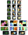 |
Fig. B.2. continued. |
The best-fitting Ai, λ0, i, and σi for each spaxel i are found with the Levenberg-Marquardt algorithm. For the fitting we use the framework provided by astropy.modelling (Astropy Collaboration 2022). The initial parameter guesses for the algorithm are derived from the data itself – for λ0, i and σi via the first- and second moment and for Ai via the peak value of the observed line profile. For each spaxel the best-fit λ0, i and σi are then converted into vlos, i and σobs, i in km s−1 via
 (B.2)
(B.2)
and
 (B.3)
(B.3)
where  is the average of all reliable λ0, i fits and
  relates to resolving power Ri = λ0, i/FWHMLSF, i at λ0, i for each spaxel i. We note that cosmic ray hits severely hampered the line fits for some galaxies that were observed only with a single exposure. We mask the affected spaxels manually. This results in a few gaps in the velocity field (see, e.g. eLARS 4 and eLARS 11 in Fig. B.1 for the worst cases).
To measure Ri we first extract the HgNe arc-lamp exposures that flanked each observation. Then, we fit Gaussians to the Ne lines of the lamp that are blue- and red of the galaxies Hα lines (6717 Å and 6929 Å) for each spaxel. Lastly, we interpolate linearly between these so determined widths to the wavelength λ0, i of the galaxies Hα emission. In Table A.1 we list for each target galaxy the average R over all spaxels that have reliable Hα profiles. As already demonstrated in H16, R varies typically by a factor 1.5 over the FoV, and the pattern depends on where the telescope was pointing (cf. Fig. 2 in H16).
To quantify whether a fit is reliable or not we estimate the fit parameter uncertainties via a Monte-Carlo simulation. Here each spaxel is perturbed according to the corresponding error vector from the data reduction and then fitted again. This process is repeated 103 times and then the standard deviation of the resulting distributions for each parameter A, vlos, and σ0 define the associated uncertainties ΔA, Δvlos, and Δσ0, respectively. We define the signal-to-noise ratio for each fit as S/N = Aσ/(ΔAΔσ). By visually inspecting the quality of the fits we find that spaxels with S/N ≥ 6 provide us with reliable fits over the whole sample. By evaluating the statistics of all those reliable fits (3473) via linear regression in (log10(S/N) , log10(Δσv))-space we obtain the scaling relations Δσ0 = 45.8 km s−1 × (S/N)−0.93 and Δvlos = 44.6 km s−1 × (S/N)−0.91 for the statistical uncertainties of the line-of-sight kinematical parameters. These scaling laws can be used in Fig. 1 to visually estimate the uncertainties in the vlos and σ0 maps by using their corresponding S/N map.
Moreover, as shown by Landman et al. (1982), the statistical uncertainties Δσ0 and Δvlos from least-square fitting of Gaussians to noisy intrinsic Gaussian profiles are expected to be related to S/N and σ0 via
 (B.4)
(B.4)
(see also Lenz & Ayres 1992). We test whether these scaling laws hold for our data by linear regression to the relations
![Mathematical equation: $$ \begin{aligned} \Delta v_\mathrm{los} = A_{v_\mathrm{los} } \left( \frac{1}{2} \log _{10}(\sigma _0 [\mathrm {km\,s}^{-1}]) - \log _{10}(S/N) \right) + B_{v_\mathrm{los} } \end{aligned} $$](/articles/aa/full_html/2025/01/aa51012-24/aa51012-24-eq201.gif) (B.5)
(B.5)
and
![Mathematical equation: $$ \begin{aligned} \Delta \sigma _0 = A_{ \sigma _0} \left( \frac{1}{2} \log _{10}(\sigma _0 [\mathrm {km\,s}^{-1}]) - \log _{10}(S/N) \right) + B_{ \sigma _0} \end{aligned} $$](/articles/aa/full_html/2025/01/aa51012-24/aa51012-24-eq202.gif) (B.6)
(B.6)
to the results from all 3473 reliable fits from all eLARS galaxies. The linear regressions result in
 (B.7)
(B.7)
and
 (B.8)
(B.8)
The relations of Eq. (B.5) and Eq. (B.6) with the determined coefficients in Eq. (B.7) and Eq. (B.8) are in near perfect agreement with the expected relations of Eq. (B.4).
Lastly, the adequateness of the Gaussian profiles is also visually checked for each of the 3473 fits. As anticipated from above steps, for most of the galaxies, the information content in the observed Hα profiles per PMAS spaxel is optimally summarised by the three Gaussian parameters. Exceptions are the galaxies eLARS 7 and eLARS 24 where numerous spaxels in both galaxies show clear double component Hα profiles. These complicated profiles lead to inflated σ0 values in the fits and, moreover, this kinematical complexity is lost in our vlos and σ0 maps. Accordingly, we also exclude LARS 9 and LARS 13 from the H16 sample, as both of these galaxies also exhibit double component profiles. We excluded all galaxies with double component profiles from statistical analyses that involve  and vshear/σ0obs.
Appendix C: Measurement of the intrinsic dispersion
The analysis presented in this work requires measurements of the intrinsic velocity dispersion of the Hα emitting gas. This quantity, σ0, is defined as a galaxy’s average isotropic velocity dispersion. Simple empirical and model-independent estimates of σ0 from observed velocity dispersion maps, σx, y, are the mean,
 (C.1)
(C.1)
or the weighted mean,
 (C.2)
(C.2)
where N is the number of spaxels that can be used. As weights one can adopt the fluxes or the S/N’s (since S/N∼ flux) of the emission line in each spaxels. The flux weighted mean was used in H16 for the LARS galaxies.
The finite size of a spaxel and the convolution of the galaxy’s observable Hα emission with the atmospheric point spread function lead to a broadening of the measured σi, when the spaxel i is at the position of a steep velocity gradient. In analogy to radio astronomy, where a broadening of line widths occurs due to the finite size of the beam, this broadening is sometimes named “beam smearing effect” (Davies et al. 2011; Varidel et al. 2016). The simple measures σm, u and σm, w are thus biased high for galaxies that show strong gradients. Particularly in disc galaxies, the intrinsic rotation is steepest near the bright centre of the galaxy, and therefore σm, u appears not to be an ideal measure for the combined LARS and eLARS samples due to its significant fraction of disc- (RD) and disc-like (PR) galaxies (73 %; Sect. 3.2.1).
Kinematical modelling that accounts for the spatial and instrumental broadening of the observed emission line signal in the datacube, appears to be the most reliable method to obtain a measure of σ0 (Davies et al. 2011; Bouché et al. 2015; Varidel et al. 2019). However, for CK and PR galaxies such modelling cannot produce reliable results, as their kinematics are not captured by simple parametric models11. Thus, the method can only be applied to less than half of our sample, as it contains 57% CKs and PRs (Sect. 3.2.1). Our approach is therefore to rely on an empirical method that performs best when compared against the results from kinematical modelling of the RD subsample. For the modelling of the RDs we use the GalPak3D software (Bouché et al. 2015) and we assert that the recovered dispersion of the model, σGP, represents the ground truth.
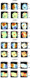 |
Fig. C.1. Comparison between observed (left column) and modelled (middle column) line-of-sight velocity field (top row for each galaxy) and velocity dispersion maps (bottom row for each galaxy). The difference between observations and model are shown in the right column. |
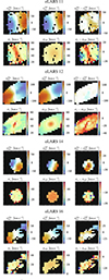 |
Fig. C.1. continued. |
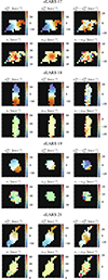 |
Fig. C.1. continued. |
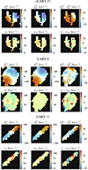 |
Fig. C.1. continued. |
Kinematical parameters from GalPak3D modelling
Summarising statistics of the residual maps vobs − vGP and σv − σGP shown in Fig. C.1.
The details on our GalPak3D modelling are given in Appendix C.1. We then present several empirical methods in Appendix C.2 before we asses their performance in Appendix C.3.
C.1. GalPak3D modelling
GalPak3D (Bouché et al. 2015) uses a Markov chain Monte Carlo technique to find the parameter uncertainties of a disc model given the line emission in the IFS datacube. The defining feature of GalPak3D is that the comparison between model and data is directly evaluated on the datacube. Broadening by the instrument’s line spread-function (LSF) and the effect of seeing are accounted for in the modelling by convolution with a 1D and 2D Gaussian, respectively. The width parameters of these Gaussians have to be provided as input parameters for the model. As mentioned in Appendix B, the width of the LSF varies slightly over the PMAS field-of-view. We here use the mean LSF width as input parameter (according to the R values provided in Table A.1). For the 2D Gaussian that mimics the seeing, we use the average DIMM measure for each observation, also provided in Table A.1. For simplicity, we also chose to model only galaxies that fit within one PMAS 16″×16″ pointing, i.e. we excluded eLARS 05 from the modelling. We furthermore exclude eLARS 24 from the modelling due to its double component Hα profiles (Sect. 3.1).
Log of Calar-Alto 3.5m PMAS eLARS observations.
The parametric model assumes the radial light distribution of the disc to follow an exponential profile, I(r) = Ieexp(−b1[(r/Re)−1]), with free parameters Re and Ie, i.e. the half-light radius and the surface-brightness at Re (this is ensured via the constant b1 = 1.678; Graham & Driver 2005). The vertical light distribution of the disc is assumed as exponential, I(z)∝exp(−z/hz), where hz is fixed to hz = 0.15Re. As rotation curve we chose the empirical tanh-profile, v(r) = Vmaxtanh(r/Rt), with the maximum velocity, Vmax, and the turnover radius, Rt, being the free parameters. The velocity distribution of the disc is modelled in GalPak3D as three terms that are added in quadrature,  , where the first term is the local isotropic velocity dispersion driven by self-gravity, σGP, g(r)/hz = v(r)/r, the second term, σGP, m, is a mixing term that arises due to projection effects, and the third term is the for our analysis required isotropic and homogeneous dispersion term σGP, 0. The model contains three additional free parameters, namely the 3D coordinates of the rotating discs centre.
We list the final results of the disc parameters obtained with the modelling in Table C.1 and in Fig. C.1 we compare the observed line of sight velocity and velocity dispersion maps against the maps produced by GalPak3D. Moreover, we summarise the level of congruity between the line of sight velocity and dispersion maps in Table C.2. There we list the mean of the absolute deviations over all spaxels, Δv, GP = ⟨|vobs, i − vGP, i|⟩, as well as the standard deviation, stdv, GP = std(|vobs, i − vGP, i|), to quantify the match between observed and modelled velocity field. To quantify the match between the observed dispersion maps and the dispersion maps recovered from the model, we provide the mean, Δσ, GP = ⟨σobs, i − σGP, i⟩, and the standard deviation, stdσ, GP = std(σobs, i − σGP, i), over the residual maps in Table C.2.
As can be seen from this comparison, for most of the galaxies the simple parametric model results in line of sight velocity maps that capture qualitatively the large-scale kinematics of the Hα emitting gas. However, for none of our galaxies the residuals appear as spatially randomly distributed noise, instead they appear to indicate genuine kinematical features that are not captured by the simple parametric model. The amplitude of these deviations from the simple disc model are, however, significantly smaller than the overall observed shearing amplitudes. With Δv, GP < 10 km s−1, the best level of congruities are found in eLARS 6, eLARS 8, eLARS 17, and eLARS 18, whereas the largest incongruities are found for LARS 11 with Δv, GP ≈ 30 km s−1. The situation is slightly different for the velocity dispersion maps. While here a few galaxies display also structures within the residuals that are likely kinematical features not captured by the simple model (eLARS10 and eLARS 11 are prominent examples), for other galaxies the residual maps appear to indicate indeed random noise (e.g. eLARS 8 and eLARS 17). Nevertheless, the overall match between observed and modelled dispersions is satisfactory, with the absolute mean |Δσ, GP|≲5 km s−1 for most of the sample, albeit the model tends to result in slightly higher dispersions. The standard deviation of the residual maps is typically 10 km s−1.
The main application of GalPak3D is the modelling of spatially unresolved high-z discs. Given that the here modelled low-z galaxies are spatially resolved into individual substructures, a perfect match between model and observations is not expected. A better fit might be achieved by a model that incorporates the complex gas structure (i.e. BLOBBY3D; Varidel et al. 2019). Still, the overall congruence between recovered and observed line of sight velocity fields and velocity dispersion maps is quite encouraging. This is in line with the recent application of GalPak3D modelling of low-z low-metallicity star-forming galaxies by Isobe et al. (2023). We thus use σ0, GP values as our ground truth and, given the presented statistics of the residual maps, consider an empirical method as successful in recovering the truth, if it is on average within 10 km s−1 of the dispersion values from the model.
C.2. Empirical methods
Empirical estimates of the intrinsic velocity dispersion (in km s−1) obtained with the methods described in Appendix C.2.
The simplest heuristic method for estimating the intrinsic velocity dispersion are the means introduced already in Eqs. (C.1) and (C.2). We list in Table C.3σm, u and σm, w according to those equations. For σm, w we use the S/N as weights in the calculation. We also provide in Table C.3 the number of spaxels, N, that contribute to the respective means.
As mentioned, the simple- and the weighted mean can be biased high due to beam smearing. A conceptually straight forward workaround is masking out spaxels in the calculation of σm, w and σm, u that are significantly affected by the PSF induced line broadening. As these spaxels are in the vicinity of strong velocity gradients, we here introduce a gradient-like measure for each spaxel, vg, calculated with respect to all eight neighbouring spaxels on the observed line of sight velocity map. Our gradient-like map is thus defined by
![Mathematical equation: $$ \begin{aligned} v_g(x,y) = \sqrt{ \sum _{i = (-1, 0, +1)} \sum _{j = (-1, 0, +1)} [v_{x-i,y-j} - v_{x,y}]^2 } \;\text{.} \end{aligned} $$](/articles/aa/full_html/2025/01/aa51012-24/aa51012-24-eq213.gif) (C.3)
(C.3)
Empty spaxels, i.e. spaxels that did not meet the signal-to-noise criterion or were affected by cosmic-ray hits (Sect. 3.1), are set to zero in the calculation. We show the so obtained vg(x, y) maps for the eLARS galaxies in Fig. C.2. We then define a binary mask,
 (C.4)
(C.4)
to calculate masked versions of the mean (Eq. C.1),
 (C.5)
(C.5)
and the weighted mean (Eq. C.2),
 (C.6)
(C.6)
respectively. Based on visual inspection of Fig. C.2, and by iteratively assessing the performance of σm, ugrad and σm, wgrad against σGP, 0 from the GalPak3D modelling (Sect. C.3), we settled on a masking threshold of vg, thresh = 70 km s−1.
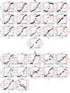 |
Fig. C.3. Radial line of sight velocity profiles (left axes, black crosses) and velocity dispersion profiles for (right axes, red circles) for the RD (top panels) and PR (bottom panels) galaxies. The position angle is shown in the bottom right of each panel. Vertical lines show the radius beyond which the velocity dispersion measurements were not deemed to be affected by PSF smearing. |
We list in Table C.3 the σm, ugrad and σm, wgrad computed with Eq. (C.5) and Eq. (C.6), respectively, alongside the number of masked spaxels, Nmasked, for which vg(x, y) > 70 km s−1. For galaxies without large shearing amplitudes within a small solid angle, we have vg(x, y) < 70 km s−1 for all spaxels, which is why Nmasked = 0, and therefore σm, ugrad ≡ σm, u and σw, ugrad ≡ σm, ugrad. For galaxies where Nmask > 0, we always have σm, wgrad < σm, w and σm, ugrad < σm, u. In these cases the corrections of both means from the masking are mostly small (≲5 km s−1) with the exceptions being LARS 3 and eLARS 24, where the correction amounts to 24 km s−1 (35 km s−1) and 12 km s−1 (22 km s−1) for the weighted (unweighted) mean. The latter galaxy shows strongly double peaked Hα emission, however the mask actually covers the spaxels, resulting in a strong downward correction due to the exclusion of the artificially broadened spaxels. LARS 3 (cf. Fig. 5 in H16), on the other hand, is a perturbed rotator with a large shearing amplitude and here numerous spaxels that appear to be severely affected by beam smearing get masked.
Varidel et al. (2016) made an alternative suggestion to correct empirically for the beam smearing effect. According to their method, one starts by calculating a gradient-like measure similar to Eq. (C.3), but only using the 4-connected topology, that is,
 (C.7)
(C.7)
This measure is then fitted to a linear 2D model that expresses σx, y as combination of a constant term, a linear term in flux, and a linear term in vgV16(x, y):
 (C.8)
(C.8)
The rationale beyond Eq. (C.8) is, according to Varidel et al. (2016), that beam smearing will be dependent on the received flux and the velocity gradient. A beam-smearing corrected map of velocity dispersion is then obtained by fitting Eq. (C.8) to each spaxel, before creating a beam-smearing corrected map from the fits by setting mvg ≡ 0: σx, yV16 = mHα ⋅ log10(FHα)x, y + c. Then, the mean, σm, uV16, and the weighted mean, σm, wV16, are calculated via Eq. (C.1) and Eq. (C.2), where σx, yV16 is used instead of the observed σx, y. We list the so obtained values for σm, uV16 and σm, wV16 in Table C.3. Both the σm, uV16 and σm, wV16 values are significantly smaller than the other empirical measures introduced above.
As final empirical method we here test the scheme put forward by Yu et al. (2021) (see also Wisnioski et al. 2015). The ansatz of this method is to avoid spaxels affected by beam smearing via a visual inspection of the radial line of sight velocity profile along the kinematical major axis. Following Yu et al. (2021), we extract the kinematical major axis from our line of sight velocity fields with the tool fit_kinematic_pa12 (Krajnović et al. 2006). The line of sight velocity profiles and velocity dispersion profiles are then created by considering spaxels ±1.5″ above and below the kinematical major axis. We show the so obtained line of sight velocity profiles and velocity dispersion profiles for the RDs and PDs in our sample in Fig. C.3. Yu et al. (2021) suggest to visually inspect the profiles to define a radius where beam smearing is not deemed to be relevant, i.e. ideally where the rotation curve becomes flat. We follow this method, but note that for some galaxies we do not sample the flat part of the rotation curve. However, for those galaxies the velocity gradient also appears to be shallower, and thus the spaxels are not as strongly affected by PSF smearing. Averaging the measured dispersions (red points in Fig. C.3) in the outer part of the velocity dispersion profiles then provides us with empirical velocity dispersion that we denominate σYu21. We tabulate σYu21 alongside the other empirical velocity dispersion measures in Table C.3. For most of the analysed galaxies σYu21 is larger than the weighted and unweighted dispersions according to the Varidel et al. (2016) method, but smaller than the other empirical dispersion measures.
C.3. Which empirical method performs best?
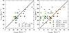 |
Fig. C.4. Comparison between velocity dispersions calculated with the empirical methods and the velocity dispersion from the GalPak3D modelling. For each method the 𝒫 measure from Eq. (C.9) is given in the legend. |
Difference (in km s−1) between velocity dispersions calculated with the empirical methods and the intrinsic velocity dispersion σGP, 0 of the GalPak3D models. The last row shows 𝒫 according to Eq. (C.9).
We assessed the performance of the empirical methods by comparing them to the velocity dispersion from the GalPak3D model. We use the metric introduced by Davies et al. (2011) for this purpose:
![Mathematical equation: $$ \begin{aligned} \mathcal{P} = \mathcal{S} \left[ \frac{1}{n} \sum _{k = 1}^{n} \left( \sigma _\mathrm{emp} ^k - \sigma _\mathrm{GP,0} ^k \right)^2 \right]^{1/2} \;\text{,} \end{aligned} $$](/articles/aa/full_html/2025/01/aa51012-24/aa51012-24-eq219.gif) (C.9)
(C.9)
where 𝒮 = ⟨σempk − σGPk⟩/|⟨σempk − σGPk⟩| is either +1 or −1 depending on whether the empirical velocity dispersions are, on average, an underestimate or overestimate of the true velocity dispersion, respectively. The sum in Eq. (C.9) runs over all galaxies. For each galaxy we list in Table C.4 the individual differences, σemp − σGP, 0 for every empirical method discussed in the previous section. A graphical comparison is given in Figure C.4. The values for 𝒫 are given both in the legend of Figure C.4 and in the last row of Table C.4.
As discussed above (Appendix C.1), we consider methods as useful if they result in |𝒫|< 10 km s−1. Our comparison shows that the method proposed by Varidel et al. (2016) severely underestimates the velocity dispersion. The ad hoc parameterisation of the beam-smearing effect proposed by those authors appears thus to over correct the actual bias. On the other hand, the method adopted by Yu et al. (2021) performs excellent for most galaxies, with |σYu21 − σGP, 0|< 5 km s−1 for 9 out of 15 galaxies, and 𝒫 = −7.1 km s−1. This method thus fulfils our acceptance criterion of 10 km s−1, but unfortunately it is not applicable to the CK galaxies of our sample.
Fortunately, we find an acceptable positive bias for the weighted and unweighted mean, and the bias even slightly decreases by 1 km s−1 when our masking scheme (Eqs. C.3–C.6, with vg, thresh = 70 km s−1) is applied (see last four columns in Table C.4). Based on this analysis, we thus adopt σm, ugrad as our observational estimate,  , of the intrinsic velocity dispersion for our analysis.
Appendix A: Hα kinematical parameters of eLARS
We tabulate in Table D.1 the kinematical parameters that have been derived in Sect. 3.2.1, 3.3, and Appendix C.1.
We also list in Table D.1 the integrated velocity dispersion σtot. We obtain σtot by calculating the square root of the second central moment of the Hα profile that is obtained by summing all spaxels with S/NHα ≥ 6. This measure provides a useful comparison with observations that do not resolve the kinematics on the spatial scales probed here, e.g. H I observations where the beam-size is close to the FoV of the PMAS observations or measurements of unresolved galaxies at high z. This column in Table D.1 is provided for reference and we do not use this quantity in the analyses presented in this paper.
Appendix E: Robustness of the correlations
Throughout we used the Kendall’s τ (e.g. Puka 2011) to measure the strength of a possible monotonic relation between two sets of observables. In order to treat upper limits in these calculation we follow the formalism of Isobe et al. (1986). To derive error-bars for the correlation coefficients and to asses their robustness we follow Curran (2014) and perform a Monte-Carlo simulation13.
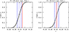 |
Fig. E.1. Examples of the adopted methodology to assess the robustness of the correlations presented in Appendix E. Both panels show the cumulative distribution of Kendall’s τ obtained from 104 Monte-Carlo simulations, where for each realisation the involved variables were perturbed according to their error-bars. The green dotted line shows the median of the distribution, which is adopted to calculate p0, whereas the blue dashed lines show the upper- and lower quartile. The solid red line shows the critical τ value according to Eq. (E.2). Both panels show the cumulative distribution of τ for the relation between vshear/σ0obs and |

Overview of the global kinematical parameters derived from the PMAS observations of the LARS+eLARS galaxies.
In our simulation we generate 104 new sets of observations of our sample with each datum being perturbed according to its uncertainty. We then analyse the resulting distributions of τ-values from this simulation. The quoted τ values always refer to the median of the distribution. Their error-bars are derived from the interquartile-range, q75 − q25, via the relation  , where erf−1(x) denotes the inverse of the error function erf(x). The p0 value is calculated from the median of the distribution in τ’s from the Monte-Carlo experiment. We use the approximation that the distribution under the null-hypothesis of no correlation (i.e. random pairings of the N observables) in
  is normal. In this case the expected variance of τ is given by Var(τ) = (4N + 10)/(9N(N − 1)). This allows for a closed form expression of p0 for the two-tailed test:
 (E.1)
(E.1)
We deem a correlation as robust if the upper- (q75) or lower quartile (q25) does not overlap with the threshold in τ that corresponds to a p-value. Again assuming a normal distribution of  under the null-hypothesis, this allows for a closed expression of the threshold:
 (E.2)
(E.2)
with erfc−1(p0) denoting the inverse of the complementary error function of p0. In our study we encounter the following sample sizes: N = {42, 38, 33, 15}. For these N, and adopting p0 = 0.05, Eq. (E.2) then results in the thresholds14 |τ|> {0.210, 0.221, 0.239, 0.337}. These different N or τ values correspond to analyses involving vshear as one parameter, analyses involving  or vshear/σ0obs (i.e. excluding galaxies with double component profiles) as one parameter, analyses excluding all upper limits in the Lyα observable (i.e. all analyses presented in Sect. 4.1), and correlation analyses that rely on measured kinematic inclinations (Sect. 3.4), respectively.
To exemplify this procedure we show in Figure E.1 two cumulative distributions of τ’s from the Monte Carlo simulation – one for which the correlation is found to be robust (left panel) and one for which the correlation is found not to be robust (right panel).
Appendix F: Extinction corrected starburst ages
In M23 we provided a global starburst age estimate that was weighted by the FUV luminosities. However, this age estimate is biased towards regions that show no or little extinction. Since star clusters form in dusty regions, this age estimate may thus biased towards older populations that have cleared their natal dust reservoirs. When analysing the age dependence of  , EWLyα, and
  in Sect. 4.2.1 we instead opted for using an age estimate that is weighted by the dust corrected UV continuum luminosity. In Table F.1 we provide these new age estimates, and in Figure F.1 we compare the new extinction corrected age estimates to the values provided in M23. As in M23 we compute the error-bars on the age estimates by a Monte-Carlo simulation, where the photometric measurements in each Voronoi cell are perturbed by the corresponding error estimates. As anticipated, for the majority of galaxies we obtain younger ages when weighing the age estimates by the dust-corrected UV luminosities.
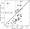 |
Fig. F.1. Comparison of extinction corrected UV luminosity weighted starburst ages to UV luminosity weighted ages from M23. Filled points indicate the sample used for all statistical analyses, i.e. excluding galaxies without double component Hα profiles and galaxies without upper limits in their Lyα observables; the latter are shown as open symbols. The one-to-one relation is indicated as a solid black line and we label the nine galaxies where the dust-corrected age estimate is larger than the new age estimate. |
Extinction corrected UV luminosity weighted ages.
All Tables
LARS+eLARS galaxy parameters against which the importance of vshear, , and vsehar/σ0obs for regulating EWLyα, , and LLyα is assessed.
Summarising statistics of the residual maps vobs − vGP and σv − σGP shown in Fig. C.1.
Empirical estimates of the intrinsic velocity dispersion (in km s−1) obtained with the methods described in Appendix C.2.
Difference (in km s−1) between velocity dispersions calculated with the empirical methods and the intrinsic velocity dispersion σGP, 0 of the GalPak3D models. The last row shows 𝒫 according to Eq. (C.9).
Overview of the global kinematical parameters derived from the PMAS observations of the LARS+eLARS galaxies.
All Figures
|
Fig. 1. Hα kinematics of four eLARS galaxies from PMAS (16″ × 16″ field of view). For each galaxy we show HαS/N (left panels; colour coded in log-scale from 1 to 1000), vlos [km s−1] (centre panels; velocities are colour coded linearly from blue (approaching) to red (receding) with the centre at vlos = 0 in white and scaled symmetrically to the absolute maximum), and σv [km s−1] (right panels; colour coded linearly from the 2nd percentile to the 98th percentile of the observed σv distribution per galaxy). The name of each galaxy is coloured according to the visual kinematic classification (Sect. 3.2): rotating discs in purple, perturbed rotators in green, and galaxies with complex kinematics in orange. The full sample is shown in Appendix B (Fig. B.1). |
| In the text | |
|
Fig. 2. Stacked histograms, colour coded according to kinematical class (rotating discs: purple; perturbed rotators: green; complex kinematics: orange) of the Lyα observables EWLyα (left panel), |
| In the text | |
|
Fig. 3. Stacked histograms of the global kinematical measures vshear (left panel), |
| In the text | |
|
Fig. 4. Lyα observables (top panel: LLyα; middle panel: EWLyα; bottom panel: |
| In the text | |
|
Fig. 5. Stacked histograms, colour-coded according to kinematical class (as in Fig. 2) of M⋆ (left panel) and SFRHα (right panel) from M23. |
| In the text | |
|
Fig. 6. Global kinematical measures vs. stellar mass (left panels) and star-formation rate (from Hα; right panels) for the LARS (squares) and eLARS galaxies (circles). The left-hand top-, middle-, and bottom panels show vshear vs. M⋆, σ vs. M⋆, and vshear/σ0obs vs. M⋆, respectively. The right-hand top-, middle-, and bottom panels, show vshear vs. SFRHα, |
| In the text | |
|
Fig. 7. Relations between ionised gas kinematics (vshear, |
| In the text | |
|
Fig. 8. Importance of observational and physical parameters for |
| In the text | |
|
Fig. 9. Correlation matrix heat map visualisation (Kendall’s τ) for observational parameters (left panel) and physical parameters (right panel), including vshear, |
| In the text | |
|
Fig. 10. Visualisation of the parameter importance for responses EWLyα (top panels), fescLyα (middle panels), and LLyα (bottom panels) from a conditional perspective using step-wise regression in a multivariate linear regression framework (see Sect. 4.1.2 for details). The panels on the left- and right-hand sides visualise the distribution of rankings p(r(xi)) for the parameters xi from the observational and physical parameter sets, respectively, where each set includes the kinematical parameters that have been derived in this work. Low values of r(xi) indicate a high importance of xi, whereas high values indicate a low importance. All but two of the curves were obtained using a kernel-density estimator (Gaussian kernel, width = 0.5) on the ranks from NMC = 103 Monte Carlo realisations. The exceptions are the |
| In the text | |
|
Fig. 11. Relations between |
| In the text | |
|
Fig. 12. Lyα equivalent width, EWLyα, vs. nebular extinction, E(B − V). Points are coloured according to |
| In the text | |
|
Fig. 13. Lyα escape fraction, |
| In the text | |
|
Fig. 14. Lyα/Hα ratio against the Hα/Hβ luminosity ratio for the in Sect. 4 analysed subsample of 33 galaxies as. there is no correlation between both quantities (τ = −0.09/pτ = 0.47). Symbols, colouring, and highlighting of the symbols is the same as in Fig. 13. The expectation of Lyα/Hα as a function of Hα/Hβ for a homogeneous dust-screen without radiative transfer effects in front of the line emission is shown as a solid line (Eq. (6)). The curves with a colour gradient indicate possible values for Lyα/Hα and Hα/Hβ for a clumpy dust screen, where on average NC = {3, 7, 9} clumps block the sight lines (Eq. (9)). These lines are drawn with a colour gradient that indicates the dust optical depth τC at 1216 Å of a single clump (colour bar at the top of the plot). |
| In the text | |
|
Fig. 15. Lyα escape fraction, |
| In the text | |
|
Fig. B.1. Hα kinematics of eLARS from PMAS (16″×16″ field of view). For each galaxy we show HαS/N (left panels; colour coded in log-scale from 1 to 1000), vlos [km s−1] (centre panels; approaching to receding velocities are colour coded linearly from blue to red with the centre at vlos = 0 in white and scaled symmetrically to the absolute maximum), and σv [km s−1] (right panels; colour coded linearly from the 2th-percentile, median, and 98-th percentile of the observed σv distribution per galaxy). The name of each galaxy is coloured according to the visual kinematic classification (Sect. 3.2): rotating discs in purple, perturbed rotators in green, and galaxies with complex kinematics in orange. Galaxies with two PMAS pointings are assembled at the bottom of this two-page figure. |
| In the text | |
|
Fig. B.2. continued. |
| In the text | |
|
Fig. C.1. Comparison between observed (left column) and modelled (middle column) line-of-sight velocity field (top row for each galaxy) and velocity dispersion maps (bottom row for each galaxy). The difference between observations and model are shown in the right column. |
| In the text | |
|
Fig. C.1. continued. |
| In the text | |
|
Fig. C.1. continued. |
| In the text | |
|
Fig. C.1. continued. |
| In the text | |
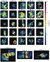 |
Fig. C.2. Gradient maps according Eq. (C.3) for the eLARS galaxies. |
| In the text | |
|
Fig. C.3. Radial line of sight velocity profiles (left axes, black crosses) and velocity dispersion profiles for (right axes, red circles) for the RD (top panels) and PR (bottom panels) galaxies. The position angle is shown in the bottom right of each panel. Vertical lines show the radius beyond which the velocity dispersion measurements were not deemed to be affected by PSF smearing. |
| In the text | |
|
Fig. C.4. Comparison between velocity dispersions calculated with the empirical methods and the velocity dispersion from the GalPak3D modelling. For each method the 𝒫 measure from Eq. (C.9) is given in the legend. |
| In the text | |
|
Fig. E.1. Examples of the adopted methodology to assess the robustness of the correlations presented in Appendix E. Both panels show the cumulative distribution of Kendall’s τ obtained from 104 Monte-Carlo simulations, where for each realisation the involved variables were perturbed according to their error-bars. The green dotted line shows the median of the distribution, which is adopted to calculate p0, whereas the blue dashed lines show the upper- and lower quartile. The solid red line shows the critical τ value according to Eq. (E.2). Both panels show the cumulative distribution of τ for the relation between vshear/σ0obs and |
| In the text | |
|
Fig. F.1. Comparison of extinction corrected UV luminosity weighted starburst ages to UV luminosity weighted ages from M23. Filled points indicate the sample used for all statistical analyses, i.e. excluding galaxies without double component Hα profiles and galaxies without upper limits in their Lyα observables; the latter are shown as open symbols. The one-to-one relation is indicated as a solid black line and we label the nine galaxies where the dust-corrected age estimate is larger than the new age estimate. |
| In the text | |
Current usage metrics show cumulative count of Article Views (full-text article views including HTML views, PDF and ePub downloads, according to the available data) and Abstracts Views on Vision4Press platform.
Data correspond to usage on the plateform after 2015. The current usage metrics is available 48-96 hours after online publication and is updated daily on week days.
Initial download of the metrics may take a while.