| Issue |
A&A
Volume 683, March 2024
|
|
|---|---|---|
| Article Number | A11 | |
| Number of page(s) | 58 | |
| Section | Extragalactic astronomy | |
| DOI | https://doi.org/10.1051/0004-6361/202347977 | |
| Published online | 28 February 2024 | |
Radio-continuum spectra of ram-pressure-stripped galaxies in the Coma Cluster
1
Leiden Observatory, Leiden University, PO Box 9513, 2300 RA Leiden, The Netherlands
e-mail: iroberts@strw.leidenuniv.nl
2
National Centre for Radio Astrophysics, Tata Institute of Fundamental Research, Post Box 3, Ganeshkhind PO, Pune 411007, India
3
Department of Physics & Astronomy, University of Alabama in Huntsville, 301 Sparkman Drive, Huntsville, AL 35899, USA
4
Research Center for Intelligent Computing Platforms, Zhejiang Laboratory, Hangzhou 311100, PR China
5
INAF – Padova Astronomical Observatory, Vicolo dell’Osservatorio 5, 35122 Padova, Italy
6
Hamburger Sternwarte, Universität Hamburg, Gojenbergsweg 112, 21029 Hamburg, Germany
7
Space Research Institute (IKI), Profsoyuznaya 84/32, Moscow 117997, Russia
8
Astro Space Center, P. N. Lebedev Physical Institute of RAS, Profsojuznaya 84/32, Moscow 117997, Russia
9
INAF – Istituto di Radioastronomia, via Gobetti 101, 40129 Bologna, Italy
10
Astronomy Data Center, National Astronomical Observatory of Japan, Mitaka, Tokyo 181-8588, Japan
Received:
15
September
2023
Accepted:
30
October
2023
Context. The population of galaxies in the local Universe is bi-modal in terms of the specific star formation rate. This fact has led to a broad distinction between star-forming galaxies (typically cold-gas-rich and late-type) and quenched galaxies (typically cold-gas-poor and early-type). The ratio between quenched and star-forming galaxies is much higher in clusters than the field, and pinpointing which are the physical processes driving this excess quenching in clusters is an open question.
Aims. We used the nearby Coma Cluster as a laboratory to probe the impact of ram pressure on star formation as well as to constrain the characteristic timescales and velocities for the stripping of the non-thermal interstellar medium.
Methods. We used high-resolution (6.5" ≈ 3 kpc), multi-frequency (144 MHz – 1.5 GHz) radio continuum imaging of the Coma Cluster to resolve the low-frequency radio spectrum across the discs and tails of 25 ram-pressure-stripped galaxies. With resolved spectral index maps across these galaxy discs, we constrained the impact of ram pressure perturbations on galaxy star formation. We measured multi-frequency flux-density profiles along each of the ram-pressure-stripped tails in our sample. We then fitted the resulting radio continuum spectra with a simple synchrotron ageing model.
Results. We show that ram-pressure-stripped tails in Coma have steep spectral indices (−2 ≲ α ≲ −1). The discs of galaxies undergoing ram pressure stripping have integrated spectral indices within the expected range for shock acceleration from supernovae (−0.8 ≲ α ≲ −0.5), though there is a tail towards flatter values. In a resolved sense, there are gradients in the spectral index across the discs of ram-pressure-stripped galaxies in Coma. These gradients are aligned with the direction of the observed radio tails, with the flattest spectral indices being found on the ‘leading half’. From best-fit break frequencies, we estimate the projected plasma velocities along the tail to be of the order of hundreds of kilometres per second, with the precise magnitude depending on the assumed magnetic field strength.
Key words: galaxies: clusters: individual: Coma Cluster / galaxies: evolution / galaxies: spiral / galaxies: starburst / galaxies: star formation / radio continuum: galaxies
© The Authors 2024
 Open Access article, published by EDP Sciences, under the terms of the Creative Commons Attribution License (https://creativecommons.org/licenses/by/4.0), which permits unrestricted use, distribution, and reproduction in any medium, provided the original work is properly cited.
This article is published in open access under the Subscribe to Open model. Subscribe to A&A to support open access publication.
1 Introduction
The Coma Cluster (Abell 1656) is the nearest massive (M200c ≲ 1015 M⊙; Ho et al. 2022) galaxy cluster to the Milky Way and is thus an invaluable laboratory for studying the effects of environmentally driven galaxy evolution. Galaxies in Coma are primarily passive, early-type galaxies, but there is a minority population of star-forming disc galaxies that are H I-deficient relative to non-cluster galaxies (e.g. Shapley 1934; Godwin et al. 1983; Gavazzi 1987, 1989; Bravo-Alfaro et al. 2000; Terlevich et al. 2001; Poggianti et al. 2004; Mahajan et al. 2010; Smith et al. 2012; Molnár et al. 2022). Among the star-forming galaxy population in Coma, multiple studies have found anomalously high star formation rates (SFRs), even compared to non-cluster galaxies (e.g. Bothun & Dressler 1986; Donas et al. 1995; Miller et al. 2009b; Roberts & Parker 2020; Roberts et al. 2021a, 2022a; Boselli et al. 2022). At a distance of ~100 Mpc, Coma is small enough on the sky (approximately a few degrees across) to be efficiently mapped by survey telescopes with degree-scale fields-of-view, but still near enough that kiloparsec physical scales can be probed with approximately arcsecond angular resolution. The combination of these two facts has led to a number of resolved studies of environmental quenching in Coma, covering a relatively large number of member galaxies. These works suggest that perturbations from ram pressure stripping are likely a key factor driving the environmental quenching observed in Coma today (e.g. Poggianti et al. 2004; Yagi et al. 2007, 2010; Smith et al. 2010; Gavazzi et al. 2018; Cramer et al. 2019, 2021; Chen et al. 2020; Roberts & Parker 2020; Roberts et al. 2021a; Lal et al. 2022).
Ram pressure stripping (e.g. Gunn & Gott 1972) is a product of the relative motion between satellite galaxies and the intracluster medium (ICM), which drives an external pressure incident on the galaxy. The efficiency of this stripping will dictate the relevant timescale for quenching star formation. In the limit of a ‘weak’ ram pressure, where only the circumgalac-tic medium and diffuse atomic gas are removed, the quenching timescale will be set by the depletion time of the surviving gas in the disc (~1 Gyr timescales; e.g. Bigiel et al. 2011; Saintonge et al. 2017). This scenario is analogous to ‘galaxy starvation’, a mechanism often cited to explain the quenching of galaxies in dense environments (e.g. Larson et al. 1980; Balogh et al. 2000; Peng et al. 2015). If ram pressure is strong enough to overcome not only the gravitational potential on the atomic gas but also the denser, centrally concentrated molecular gas component, then the star-forming gas can be stripped directly and quenching will proceed on a much shorter timescale.
Ram pressure may also alter the physical conditions of gas in star-forming regions, even if it is not directly removed from the disc. One possibility is that ram pressure compresses gas in the interstellar medium (ISM), both promoting the conversion between atomic and molecular gas and increasing the densities of existing molecular gas. Should this occur, then it would also predict enhanced SFRs in cluster galaxies, assuming a normal Kennicutt-Schmidt relation (Schmidt 1959; Kennicutt 1998). This framework has been used to explain high SFRs amongst Coma Cluster galaxies dating back four decades (Bothun & Dressler 1986); additionally, with the onset of recent large CO surveys of cluster galaxies, evidence for ram-pressure-enhanced molecular gas densities and star formation in such environments has become more widespread (e.g. Gavazzi et al. 2001; Merluzzi et al. 2013; Vulcani et al. 2018, 2020; Moretti et al. 2020a,b, 2023; Boselli et al. 2021; Cramer et al. 2021; Durret et al. 2021; Hess et al. 2022; Lee et al. 2022; Roberts et al. 2022a, 2023; Brown et al. 2023). We also note that enhanced SFRs may be a result of gas flows towards the galaxy centre, driven by ram pressure (Zhu et al. 2024). Thus, in principle, ram pressure is sufficient to explain both the aforementioned large population of quenched galaxies in Coma and the tendency for many of the remaining star-forming members to show high SFRs.
Cluster galaxies currently experiencing ram pressure stripping are generally identified in one of two ways: either by observing a one-sided tail of stripped material (e.g. Gavazzi 1978; Shostak et al. 1982; Gavazzi & Jaffe 1987; Gavazzi et al. 2001; Kenney et al. 2004; Chung et al. 2007; Yagi et al. 2010; Merluzzi et al. 2013, 2016; Poggianti et al. 2017; Boselli et al. 2018; Roberts et al. 2021a,b; Hess et al. 2022; Venturi et al. 2022; Edler et al. 2023) or (often less reliably) by identifying morphological features in the stellar light of a galaxy that are consistent with perturbations from ram pressure (McPartland et al. 2016; Poggianti et al. 2016; Roberts & Parker 2020; Durret et al. 2021; Roberts et al. 2022b; Vulcani et al. 2022). Most commonly, ram pressure tails are observationally identified through the Hα Balmer line tracing ionized gas, the 21 cm hydrogen line tracing atomic gas, or the radio continuum tracing synchrotron emission from cosmic ray electrons (CREs), with the earliest examples of late-type galaxies undergoing ram pressure stripping coming from observations in the radio continuum (Gavazzi 1978; Gavazzi & Jaffe 1987).
A primary asset of observing in the radio continuum is the large primary beam sizes, particularly at low frequencies (≲ 1 GHz), which allow for entire clusters at low redshifts to be efficiently imaged and thus galaxies undergoing ram pressure stripping to be identified across the full cluster volume. In particular, the high sensitivity (~100 µJy bm−1) and angular resolution (~6″) of the Low Frequency Array (LOFAR) Two-metre Sky Survey (LoTSS; van Haarlem et al. 2013; Shimwell et al. 2017, 2019, 2022) has led to a roughly ten-fold increase in the number of known star-forming galaxies in low-redshift groups and clusters with stripped radio tails (Roberts et al. 2021a,b, 2022c; Edler et al. 2023; Ignesti et al. 2023). In addition to being clear signs of environmental galaxy evolution, ram-pressure-stripped radio tails also deposit CREs and magnetic fields into the ICM, which contribute to the seed particle population for diffuse radio halos and relics (Ge et al. 2019).
Radio continuum emission in star-forming galaxies is a mix of thermal free-free emission from HII regions and non-thermal synchrotron emission originating from CREs accelerated by shocks from supernovae. At frequencies below ~1 GHz, the radio spectrum is dominated by the non-thermal synchrotron component. For galaxies undergoing ram pressure stripping, this includes emission from stripped tails that is believed to be tracing CREs accelerated by supernovae in the disc that are advec-tively transported out of the galaxy under ram pressure (Murphy et al. 2009; Vollmer et al. 2013; Müller et al. 2021; Roberts et al. 2021a; Ignesti et al. 2022a). For different CRE acceleration mechanisms and efficiencies, the energy spectral index, γ, for supernovae is estimated to lie in the range −2 to −2.6, which corresponds to a synchrotron spectral index, α, between −0.5 and −0.8 (γ = 2α − 1; e.g. Bell 1978; Bogdan & Volk 1983; Biermann & Strom 1993). After CREs are injected into the ISM, they are subject to energy loss mechanisms that alter α in a frequency-dependent fashion. Examples of energy loss mechanisms include ionization, synchrotron, and inverse-Compton losses. Synchrotron and inverse-Compton losses most strongly impact high-energy CREs. This acts to steepen α overall, but in particular introduces a high-frequency exponential cut-off to the (previously) power-law spectrum, occurring at the so-called break frequency (νb). If synchrotron and inverse-Compton losses are dominant, then over time the break frequency will evolve to lower frequencies and the radiative age of a given plasma can be estimated from the location of this break (e.g. Miley 1980). In the context of star formation, this means that young star-forming regions will have spectral indices that are close to the injection values (−0.8 < α < −0.5), whereas older plasma corresponding to a prior episode of star formation will be characterized by a steeper α. In the context of ram pressure stripping, radiative age estimates have been used to constrain the bulk velocity of the stripped plasma for some cluster galaxies, generally of the order of hundreds of kilometres per second (Vollmer et al. 2021; Ignesti et al. 2023).
Conversely, ionization losses flatten the spectral index by preferentially affecting low-energy CREs and thus the low-frequency portion of the spectrum. The strength of ionization losses increases with ISM density (e.g. Longair 2011), a fact that has been used to explain the flatter-than-injection spectral indices (i.e. α > −0.5) that are sometimes observed near strongly star-forming regions in galaxies (Basu et al. 2015). There is also tentative evidence for unusually flat spectral indices in the discs of galaxies undergoing ram pressure stripping (Ignesti et al. 2022b; Roberts et al. 2022c), for which ionization losses provide a potential explanation given that the compression from ram pressure is capable of increasing local ISM densities (e.g. Cramer et al. 2020; Troncoso-Iribarren et al. 2020; Moretti et al. 2020a,b; Roberts et al. 2022a, 2023; Brown et al. 2023).
A number of wide-area radio continuum surveys of the Coma Cluster have been published, spanning a decade across the low-frequency spectrum, including surveys conducted with LOFAR at 144 MHz (Shimwell et al. 2022; see also Bonafede et al. 2022), the upgraded Giant Metrewave Telescope (uGMRT) at 400 MHz and 700 MHz (Lal 2020; Lal et al. 2022), and the Very Large Array (VLA) at 1.5 GHz (Miller et al. 2009a; Chen et al. 2020). In this work we synergize data from these surveys to complete an in-depth study of the low-frequency radio spectrum of ram-pressure-stripped galaxies in Coma and their stripped tails. With a working physical resolution of ~3 kpc, and excellent sensitivity to extended, diffuse emission, we are able to probe spectral properties both across the star-forming discs and along the ram-pressure-stripped tails. From these datasets we derive constraints on ram-pressure-induced star formation, cosmic-ray losses in the ISM, and the characteristic timescales for gas stripping.
The structure of this paper is as follows: In Sect. 2 we describe the multi-frequency radio continuum imaging used in this work, as well as our sample of ram-pressure-stripped galaxies. In Sect. 3 we report integrated spectral index measurements over both galaxy discs and stripped tails. In Sect. 4 we show resolved maps of spectral index covering the galaxy discs, primarily between 144 MHz and 1.5 GHz. In Sect. 5 we measure multi-frequency flux-density profiles along observed stripped tails and apply a simple spectral ageing model to these observed radio spectra. From this model we extract estimates for synchrotron break frequencies and (projected) bulk stripping velocities along the tails. Finally, in Sects. 6 and 7 we provide a brief discussion and high-level summary of this work.
Throughout we assume a standard Λ cold dark matter cosmology with Ωm = 0.3, Ωλ = 0.7, and H0 = 70 km s−1 Mpc−1. We take the redshift of the Coma Cluster to be zComa = 0.0234 (Rines et al. 2016), which corresponds to a luminosity distance of 102 Mpc and a scale of 0.47 kpc/″. The radio synchrotron spectrum is described as Sν ∝ να, where Sν is the flux density, ν is the frequency, and α is the spectral index.
2 Data and galaxy sample
2.1 Radio imaging
2.1.1 LOFAR 144 MHz
The LOFAR images in this work are from the LoTSS (Shimwell et al. 2017, 2022), a wide-area continuum survey of the northern sky between 120 and 168 MHz using the LOFAR high-band antenna (HBA). We used three 8 h LoTSS pointings (P192+27, P195+27, P195+30) that combine to map the Coma Cluster out to the virial radius. Each pointing was processed, imaged, and mosaicked following the procedure outlined in Shimwell et al. (2022). This includes initial processing to correct for direction-independent errors, followed by direction-dependent1 calibration to account for the variation in ionospheric effects across the large field-of-view (the primary-beam full width at half maximum is ~4 deg). Direction-dependent solutions are applied during imaging with DDFacet (Tasse et al. 2018) and images for each pointing are mosaicked with neighbouring pointings in order to produce the final, mosaicked image for each field (Shimwell et al. 2022). For each field, we checked the LoTSS flux-density scale against both the TGSS (Intema et al. 2009) and 7C (Hales et al. 2007) surveys. For all three fields we measured a ~20% flux-scale offset in LoTSS, when comparing to both TGSS and 7C. When directly comparing TGSS and 7C, no flux-scale differences were measured. Thus, we applied a ~20% flux-scale correction (varying slightly from field to field) to each of the three LoTSS mosaics. The final LoTSS images for P192+27, P195+27, and P195+30 reach rms levels at the field centres of 70, 65, and 60 µJy per 6″ beam, respectively. For all frequency bands used in this analysis, we worked at a common angular resolution of 6.5″, corresponding to a physical resolution of ~3 kpc at the distance of the Coma Cluster. We convolved the LoTSS images to this working resolution using the imsmooth function in CASA (CASA Team 2022).
2.1.2 uGMRT 400 and 700 MHz
At 400 and 700 MHz we used imaging from uGMRT of the Coma Cluster from Lal (2020) and Lal et al. (2022). This imaging covers an area of ~4 deg focused on the central and south-west regions of Coma, which is made up of three pointings in Band 3 (250–550 MHz) and eight pointings in Band 4 (550–850 MHz). The on-source times range between 1.8 and 4.7 h for pointings in Band 3 and 1.3 and 3.4 h for pointings in Band 4. We refer to Lal (2020) and Lal et al. (2022) for all further details on the observing set-up.
To process the raw data we used the Source Peeling and Atmospheric Modeling pipeline (SPAM: Intema et al. 2009). We followed the recommended workflow for wide-band uGMRT data2, which first splits the dataset into ~50 MHz sub-bands that are each processed individually by the main SPAM pipeline. After processing, sub-bands were imaged together with WSClean (Offringa et al. 2014) to form a final wide-band image. For final imaging we used Briggs weighting (Briggs 1995) with a robust parameter of −0.5. This results in rms levels between 26 and 30 µJy (depending on the pointing) per ~5.5″ beam in Band 3, and rms levels between 13 and 26 µJy per ~3.5″ beam in Band 4. All Band 3 and Band 4 pointings are convolved to our working resolution of 6.5″, re-projected onto a common pixel grid, and then mosaicked together to produce a single mosaic image for each frequency band. The largest angular scale for the uGMRT is ~33′ in Band 3 and ~20′ in Band 4, both of which are much larger than the angular size of 2′ at 144 MHz for the largest source (NGC4848) in our sample.
2.1.3 VLA 1.5 GHz
For our highest-frequency data, we used two different VLA 1.5 GHz datasets, from Chen et al. (2020) and Miller et al. (2009a), which together cover more than a square degree of the Coma Cluster. Throughout this work we assumed that the observed flux density at 1.5 GHz is solely due to non-thermal, synchrotron emission - in other words, a ‘thermal fraction’ (fth) of zero. While this is unlikely to be strictly true, previous works have found typical thermal fractions of fth < 10% at 1.5 GHz for nearby star-forming galaxies (e.g. Condon 1992; Niklas et al. 1997; Tabatabaei et al. 2017; Ignesti et al. 2022b).
The observations from Chen et al. (2020) include one pointing centred on D100 and one pointing centred on NGC 4848, each well-known examples of ram-pressure-stripped galaxies in the Coma Cluster. Here we briefly highlight some main features of the data and processing and we refer to Chen et al. (2020) for a more comprehensive discussion.
The NGC 4848 and D100 fields were observed for an on-source time of 12.1 and 6.3 h, respectively, in the VLA B-configuration. Data were processed following standard procedures in CASA. After calibration, the continuum data were imaged using tclean with Briggs weighting and a robust parameter of 0.5, giving a synthesized beam size of ~4″ for both fields. At the pointing centre the resulting rms noise is 5.9 µJy bm−1 for the NGC 4848 field and 8.0 µJy bm−1 for the D100 field. Both pointings were then convolved to our working resolution of 6.5″.
The observations from Miller et al. (2009a) also include two fields, one covering the centre of the Coma Cluster (Coma 1, which has substantial overlap with the D100 field from Chen et al. 2020) and one to the south-west of the cluster centre (Coma 3). Again, here we only provide a brief description of the data processing, but a detailed outline is available in Miller et al. (2009a).
For each field, 11 separate pointings were obtained in order to achieve roughly uniform sensitivity across a 30′ × 50′ area. Each pointing was observed for ~1 h in the VLA B-configuration. The data were reduced and imaged with the Astronomical Image Processing Software (AIPS). Final images for each field have a restoring beam size of 4.4″ and reach rms levels of 20–25 µJy at the image centre. We obtained the Coma 1 and Coma 3 images from the CDS3, and both were then smoothed to our working resolution of 6.5″.
Lastly, we re-projected all four VLA images from Miller et al. (2009a) and Chen et al. (2020; after smoothing to a 6.5″ beam) onto a common pixel grid and mosaicked them together in the image plane. The image combination was weighted by the inverse of the local rms level in each image. Where the Miller et al. (2009a) and Chen et al. (2020) images overlap, the majority of the weight in the combined mosaic is thus given to the deeper Chen et al. (2020) data. In most cases, the Miller et al. (2009a) images are not deep enough to detect the stripped tails; however, these data still provide important insight into the spectral properties over the discs of galaxies not covered by the Chen et al. (2020) observations. We note that the largest angular scale for the VLA in B-configuration is 120″ for full synthesis observations4. This is nearly identical to the angular size of the largest source in our sample at 144 MHz; therefore, for the longest tails in our sample (e.g. NGC 4848 and MRK0057), it is possible that there is a small amount of missing flux density at 1.5 GHz. That said, for an ageing synchrotron population, it is expected that the observed tail length will scale inversely with the square root of the frequency (Ignesti et al. 2022b) and therefore we expect that the tails lengths at 1.5 GHz will be intrinsically shorter than at 144 MHz (by roughly a factor of three). This would bring the expected tail lengths at 1.5 GHz within the B-configuration largest angular scale.
2.2 Ram-pressure-stripped galaxy sample
Roberts et al. (2021a,b) published a large sample of ~150 galaxies with one-sided radio tails at 144 MHz that are likely undergoing ram pressure stripping in low-z groups and clusters. This sample includes 29 galaxies in the Coma Cluster.
The galaxy sample used in this work includes all ram-pressure-stripped Coma galaxies from Roberts et al. (2021a) that are also within the observing area of at least one of the 400 MHz, 700 MHz, and 1.5 GHz datasets described above. This restriction results in 23 galaxies with observations at at least two frequencies.
We also included two supplemental ram-pressure-stripped galaxies from Coma in our sample. These two galaxies, NGC4911 and KUG1258+287, were not part of the Roberts et al. (2021a) sample for technical reasons, but do show one-sided stripped tails at 144 MHz (and other frequencies). NGC 4911 is known to have an Hα stripped tail identified by Yagi et al. (2010), and also shows a clear one-sided tail in LoTSS at 144MHz (see Fig. B.8) in the same direction as the Hα tail. The reason that NGC 4911 was not included in the Roberts et al. (2021a) sample, despite the radio continuum tail, is that NGC 4911 has a specific star formation rate (sSFR = SFR/M★ = 10−11.2 yr−1) that falls just below the star-forming galaxy selection of sSFR > 10−11yr−1 imposed by Roberts et al. (2021a). However, NGC 4911 clearly shows signatures of ongoing star formation (Gregg et al. 2003; Yagi et al. 2010), and we opted to include it in our sample for completeness.
KUG1258+287 has a one-sided, ~40 kpc tail at 144 MHz in LoTSS (see Fig. B.32) but lacks a Sloan Digital Sky Survey (SDSS) redshift, presumably due to its close proximity to a bright foreground star. The Roberts et al. (2021a) sample relies on SDSS spectroscopic redshifts and therefore does not include KUG1258+287. However, KUG1258+287 does have a spectroscopic redshift of z = 0.0298 from Edwards & Fadda (2011), and thus has a projected velocity offset of ~ 1700 km s−1 from the systemic velocity of Coma. The velocity offset, alongside a projected cluster-centric radius of 0.34R180, places KUG1258+287 as a Coma member galaxy according to the criteria of Roberts et al. (2021a), and therefore we included it in our ram pressure galaxy sample.
This results in a total ram pressure stripping galaxy sample of 25 galaxies. We list these galaxies along with their general properties and frequency coverage in Table 1. In Fig. 1 we show the local rms measured from ~3′ cutout images centred on each galaxy, for each of our frequency bands. Generally speaking, we reach comparable sensitivity to freshly injected electrons in all frequency bands (α ≈ −0.7), but in most cases do not reach equivalent sensitivity in our high-frequency bands to steep-spectrum emission (α ≲ −1) detected by the LOFAR HBA. The points skewed to high rms at 1 .5 GHz in Fig. 1 correspond to those galaxies that are covered by the L-band observations from Miller et al. (2009a) but not from Chen et al. (2020).
3 Integrated spectral properties: Galaxy and tail
We measured integrated spectral indices for each galaxy disc and corresponding stripped tail in our sample. Flux densities for the galaxy disc were measured over an elliptical aperture centred on the right ascension and declination of each galaxy (see Table 1). The semi-major axis of the ellipse was taken to be the Petrosian 90% light radius (listed in Table 1) and the axis ratio and position angle were determined through 2D Sérsic fits. All structural parameters were measured in the r band and obtained from the NASA-Sloan Atlas5.
Flux densities for the stripped tails were measured over rectangular apertures that extend from the outer edge of the galaxy disc (as defined above) along the direction of the tail. The length and width of these apertures were set by hand in order to enclose tail emission within the 2σ contour at 144 MHz. We measured tail flux densities over the same aperture for each frequency band. The galaxy disc and tail apertures for each galaxy are shown in Appendix B.
A minority of galaxies in the sample overlap, in projection, with the diffuse radio halo in Coma that is well detected by LOFAR at 144MHz (Bonafede et al. 2022). Thus, direct 144 MHz flux density measurements for these galaxies will include a contribution both from CREs originating from the galaxy and from CREs originating from the radio halo. To account for this, we measured the median ‘background’ level around (but not including) each galaxy and its stripped tail. This level is then taken to be the local level of the radio halo and is subtracted off of each galaxy cutout image. The flux densities quoted in Table 2, and used throughout the rest of the paper, are then measured from images after this subtraction. While the radio halo is not detected in our 400 MHz, 700 MHz, or 1.5 GHz images, we still followed the same procedure when measuring flux densities at these higher frequencies in case there is any low-level contribution from the halo that is not immediately obvious from the images. We are implicitly assuming here that the brightness of the radio halo is constant over the length scale of the galaxy plus stripped tail (~ 10–50 kpc for our sample).
We used a threshold of 3σ to determine whether or not significant emission was detected in each aperture. If the measured flux density was below this threshold then we instead quote a 3σ upper limit. We considered two sources of error on the measured flux densities: a random error set by the noise in the image and an error on the flux calibration that is specific to each observing band. To measure the random error, we measured flux densities within 500 randomly positioned apertures in source-free regions of the image surrounding the target galaxy. We then took the random error to be the sigma-clipped standard deviation of the resulting 500 aperture flux densities. For flux calibration, we assumed a relative error of 10% for LOFAR HBA, 5% for uGMRT B3 and B4, and 5% for VLA L band. The total error on the flux density (δSν) in each aperture is then given by the sum in quadrature of the random error and the calibration error. Generally speaking, the flux calibration uncertainties are the dominant sources of error. Measured flux densities are listed in Table 2. The ‘disc + tail’ flux densities from Table 2 agree well with measured flux densities for overlapping sources from Lal et al. (2022, see their Table 3). Any small differences are due to the fact that our disc apertures, while internally consistent for this paper, do not always enclose all of the radio emission around the galaxies in our sample (see the images in Appendix B).
Spectral indices were calculated using two different methods, depending on the number of frequency bands where significant flux density was detected. When three or more frequency bands are detected, we calculated the spectral index as the slope of the best-fit linear relationship between ln S ν and ln ν. Fits are done using orthogonal distance regression, specifically scipy.odr, and the uncertainty on the spectral index is taken to be the statistical uncertainty on the best-fit slope. When only two frequency bands are detected, we calculated spectral indices via the direct method, namely
 (1)
(1)

Spectral indices for both disc and tail regions are listed in Table 2.
In Fig. 2 (top) we show the spectral index integrated over the tail versus the spectral index integrated over the disc for each galaxy in our sample. For the galaxy discs, spectral indices are broadly consistent with the typical injection spectral indices expected from star formation (approximately −0.8 to −0.5; e.g. Bell 1978; Bogdan & Volk 1983; Condon 1992). The median spectral index over galaxy discs is −0.47 ± 0.1. This agrees with the mean 144MHz – 1.5GHz spectral index of −0.55 ± 0.14 for the sample of 76 nearby star-forming galaxies from Heesen et al. (2022). Thus, we do not find evidence for different broadband spectral indices between ‘normal’ star-forming discs and galaxy discs undergoing ram pressure stripping. This is consistent with previous work in the Virgo Cluster that makes the same conclusion based off of spectral index measurements at gigahertz frequencies (Vollmer et al. 2010).
There is a collection of galaxies with spectral indices that are marginally flatter than typical injection values (i.e. >−0.5). We discuss potential origins of this spectral flattening in more detail in Sect. 6.1, but it is likely connected to increased ionization losses (due to ISM compression from ram pressure) and/or shock acceleration due to the galaxy-ISM interaction.
Spectral indices integrated over the tail region are clearly steeper than the disc spectral indices. This is true for the sample as a whole but also true for each galaxy individually. The contrast between disc and tail spectral indices is consistent with a framework where the synchrotron emission from the tail is due to aged CREs removed from the galaxy disc by ram pressure (see also: Chen et al. 2020; Müller et al. 2021; Ignesti et al. 2022b; Venturi et al. 2022). We extend our analysis of spectral ageing along the tail in Sect. 5.2, where we fit flux density profiles along the tail with a synchrotron ageing model in order to derive characteristic stripping timescales for this sample of galaxies.
There has been some evidence for flatter-than-injection spectral indices, specifically at low frequencies, in ram-pressure-stripped galaxies (Ignesti et al. 2022b; Roberts et al. 2022c). To probe whether this is the case for our sample we measured low-and high-frequency spectral indices for each galaxy disc. The low-frequency spectral index (αlow, disc) is measured between 144 and 400 MHz and the high-frequency spectral index (αhigh, disc) is measured between 700 MHz and 1.5 GHz. The results are shown in Fig. 2 (bottom) where we plot the corresponding colour-colour diagram. Given the short separations between frequency bands, the error bars on αlow, disc and αhigh, disc are large and the galaxy discs are broadly consistent with no curvature (i.e. αlow disc = αhigh disc). The median value for αlow disc is −0.43 ± 0.20 and −0.59 ± 0.24 for αhigh disc. This may be a hint of spectral curvature and flat low-frequency spectral indices in these galaxies, but we do not have the statistical power to confirm this.
Galaxy sample.
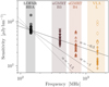 |
Fig. 1 One-sigma sensitivity (rms) as a function of frequency for each of the observing bands in this work. All values are measured from images at our working resolution of 6.5″. Data points correspond to the local rms measured around each galaxy. For the L band, the filled markers correspond to galaxies that are covered by the Chen et al. (2020) observations and the open markers correspond to galaxies only covered by the Miller et al. (2009a) observations. Shaded bands correspond to the width of each observing band. For reference, we plot lines corresponding to spectral indices of −0.5, −1, and −1.5 anchored to the lowest-frequency band. |
Flux density and spectral index measurements.
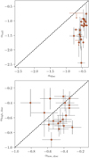 |
Fig. 2 Integrated spectral index measurements. Top: tail spectral index versus galaxy disc spectral index. When emission is detected in three or more frequency bands, the spectral index and its error are determined from orthogonal distance regression fits. When emission is only detected in two frequency bands, the spectral index and its error are determined via the direct method (Eq. (1)). For galaxies where emission in the tail is only detected at one frequency (see Table 2), αtail is shown as a 3σ upper limit. Bottom: radio colour-colour diagram for the galaxy discs. The high-frequency spectral index (y-axis) is measured between 700 MHz and 1.5 GHz, and the low-frequency spectral index (x-axis) is measured between 144 and 400 MHz. In both the top and bottom panels, the dashed lines correspond to the one-to-one relation. |
4 Disc spectral index maps
In Fig. 3 we show non-thermal spectral index maps covering the disc of each galaxy, as mentioned in Sect. 2.1.3, the thermal contribution is largely negligible at these frequencies. For the majority of galaxies, α is measured using fluxes at 144 MHz and 1.5 GHz, in order to maximize the lever arm between the two frequencies, which in turn minimizes the uncertainty of the pixel-by-pixel spectral index measurements. For galaxies that are not covered by the 1.5 GHz imaging, we measured the spectral index between 144 MHz and the highest available frequency. This corresponds to 700 MHz for KUG1250+276, and 400 MHz for KUG1257+288B, KUG1259+279, and KUG1259+284. Each panel in Fig. 3 lists the highest frequency that is used to derive the spectral index map. The disc region is defined as it was in the previous section, the r-band Petrosian 90% light radius, and is shown by the dashed lines in Fig. 3. We only include pixels in the spectral index map that have >2σ detections in both of the frequency bands that are used. For reference, when only including calibration uncertainties (which dominate over the galaxy discs), the typical uncertainty on the spectral index maps between 144 MHz and 1.5 GHz is ~0.05. For spectral index maps between 144 and 700 MHz and 144 and 400 MHz, the typical uncertainties are ~0.07 and ~0.11, respectively.
For 18 of the 25 galaxies, the spectral index at the galaxy centre (marked by the ‘x’ in Fig. 3), is consistent with values typical of recent injection from star formation (i.e. −0.8 to −0.5). The remaining seven galaxies have central spectral indices that are flatter than −0.5. In the bottom right of each panel in Fig. 3 we also show an arrow pointing in the projected direction of the radio continuum tail for each galaxy. For many galaxies in Fig. 3, the synchrotron emission is truncated within the stellar disc, which reflects the outside-in nature of ram pressure stripping. In particular, galaxies are preferentially ‘missing’ radio emission on their leading halves (i.e. opposite to the direction of the tail), corresponding to CREs being transported from the leading half along the direction of the ram pressure wind to form the stripped radio tail. This truncation is present, to varying extents, for 14/25 galaxies. Those galaxies with radio emission that fills the optical disc may represent galaxies at an earlier stage of stripping, though we note that the majority of galaxies that do not show this truncation are also only marginally resolved at 6.5’’. For these galaxies there may still be a truncated CRE distribution that is masked by the beam size. We show spectral index maps in Fig. 3, which requires detections at both frequencies, but note that this truncation signature is not a product of differences in depth between the two frequencies. When plotting single-frequency flux density maps instead, the same truncation signature is visible regardless of which frequency is used.
Across the disc there is a gradient pattern in the spectral index maps that is present for a majority of galaxies in the sample. For galaxies that show a spectral index gradient, the orientation of this gradient is roughly aligned with the direction of the stripped tail. The steepest spectral indices are generally found in the direction of the tail (relative to the galaxy centre). This pattern is consistent with cosmic rays being transported from ‘further upstream’ in the galaxy and ageing as they are transported along the tail direction. For most galaxies in Fig. 3, the flattest spectral indices are not always found at the galaxy centre, but instead are often on the leading half of the galaxy, opposite to the direction of the stripped tail. We quantitatively demonstrate this tendency for the flattest spectral indices to be found on the leading halves of galaxies by identifying the pixel in the spectral index map with the flattest spectrum, given by pixel coordinates (iflat, jflat). When determining iflat and jflat we filtered each spectral index map with a 3 × 3 uniform filter so that each pixel was averaged with its eight nearest neighbours. We also only considered pixels where all eight of the surrounding pixels have detected spectral indices, in other words we did not consider pixels on the edge of the map. Lastly, given the pixel (iflat, jflat), we calculated the radial offset of this pixel from the optical galaxy centre (rflat) as well as the angular orientation between this pixel and the direction of the radio tail (θflat). Formally, θflat is defined such that
 (3)
(3)
where uflat and utail are unit vectors pointing between the optical galaxy centre and (iflat, jflat) and away from the galaxy centre in the direction of the radio tail, respectively. In this definition, θflat= 180 deg corresponds to (iflat, jflat) being directly opposite to the tail direction and θflat > 90 deg corresponds to (iflat, jflat) being on the leading half of the galaxy disc.
In Fig. 4 we show θflat (azimuthal axis) and rflat (radial axis) for each galaxy disc on a polar plot. It is immediately clear that the distribution of θflat values does not uniformly cover the parameter space but instead is skewed towards large values, with the majority of galaxies having 120 > θflat > 180 deg and rflat offset from zero. Only for a minority of galaxies in the sample is rflat is smaller than the half width at half maximum beam size. These cases are consistent with the spectral index being flattest at the galaxy centre, and thus θflat is not particularly meaningful in this scenario.
Such an offset between the galaxy centre and the location of the flattest spectral index for galaxies undergoing ram pressure stripping was first observed for NGC 4522 in the Virgo Cluster by Vollmer et al. (2004), and seems to be relatively commonplace for such galaxies in the Coma Cluster. While a majority of galaxies show this pattern, not all do. For example, IC4040, KUG1255+275, D100, and GMP3618 all have spectral index distributions that are quite symmetric about the galaxy centre, though KUG1255+275, D100, and GMP3618 are also only marginally resolved. KUG1257+288B shows an irregular spectral index map. There is a region of flat emission on the leading half and then a second region of flat emission to the north that appears to follow a spiral arm in the galaxy (see Fig. B.26). We also note that the short frequency spacing (144-400 MHz), and the relatively low S/N detection of KUG1257+288B at 400 MHz, may be contributing to the irregular map in Fig. 3.
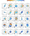 |
Fig. 3 Spectral index maps for each galaxy disc in our sample. Spectral indices are measured between 144 MHz and νmax, as listed in each figure panel. The dashed ellipse in each panel corresponds to the r-band Petrosian 90% radius, the ‘x’ marks the optical galaxy centre, and the filled circle shows the 6.5″ beam FWHM. In the lower right of each panel, we show an arrow that points in the projected direction of the stripped tail. The typical uncertainties on the spectral index maps are ~0.05 between 144 MHz and 1.5 GHz, ~0.07 between 144 and 700 MHz, and ~0.11 between 144 and 400 MHz. |
5 Spectral properties along the tail
5.1 Radio tail flux-density profiles
For each galaxy, and for each frequency band, we extracted flux-density profiles along the observed radio tail in rectangular apertures. The height (i.e. the length parallel to the tail) of each aperture is 7″ ≈ 3.5 kpc, slightly larger than the full width at half maximum (FWHM) common beam size of 6.5″, and the width (i.e. the length perpendicular to the tail) of each aperture differs from galaxy to galaxy and is set in order to enclose the lowest contour level (i.e. 2σ) shown in Appendix B. The uncertainty on flux density measurements was computed following the procedure described in Sect. 3.
The extent of the tail flux-density profiles is determined by the length of the observed tail at 144 MHz, as for all galaxies the observed tails are longest in this frequency band. The first tail aperture is set such that the inner edge of the aperture is set against the edge of the optical galaxy disc. Apertures continue along the tail in 7″ steps until significant emission is no longer detected in the 144 MHz band. We considered significant emission to be apertures where S v > 3 δS v. This approach ensures that for all flux-density profiles there is detected emission in at least one frequency band, namely 144 MHz.
In Fig. 5 we show normalized flux-density for our four frequency bands as a function distance along the tail, ℓ, which is defined such that ℓ = 0 in the first bin (i.e. just off of the galaxy disc). The flux-density profiles are normalized by the value at ℓ = 0 and therefore Fig. 5 shows the relative declines as a function of distance along the tail. We characterized the rate of this decline with a simple model of exponential decay, where the normalized flux density is given by
 (4)
(4)
where ℓs is the scale length of the flux-density decline. For each panel in Fig. 5, we fitted for the best-fit scale length in order to estimate a quantitative length scale associated with the ram pressure tails as a function of frequency. The best-fit exponential model is shown by the dashed lines in Figs. 5 and 6 we show ℓs as a function of frequency for the four bands in this work.
For a very simple model of constant stripping velocity in a constant magnetic field with no re-acceleration, one expects that the observed tail lengths will decline as the square root of the frequency (Ignesti et al. 2022b). Therefore, in Fig. 6 we also overplot the best-fit model of square-root decline as a function of frequency. This expectation broadly fits the observed scale lengths, signifying that this simple synchrotron ageing model in a relatively constant magnetic field may be a reasonable approximation to reality for our galaxy sample. Though we note that the scale length at 1.5 GHz is a 2–3σ outlier from this simple model. The scale lengths shown in Fig. 6 are derived from the full galaxy sample together and, thus, should be thought of as a description of the average behaviour for ram-pressure-stripped radio tails in Coma.
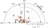 |
Fig. 4 Location of the peak (i.e. flattest) spectral index within each disc, relative to the direction of the radio tail, in polar coordinates. The azimuthal axis shows θflat, and the radial axis shows rflat (see the main text for details). The shaded region corresponds to 3.25″, the half width at half maximum of the beam. Angles greater than 90° correspond to points on the leading half (LH), and angles less than 90° correspond to points on the trailing half (TH). The peak spectral index is systematically found on the leading half (θflat > 0) of ram-pressure-stripped galaxies. |
5.2 Synchrotron ageing model
Given the support for a scenario of spectral ageing, both from the observed radial profiles and the difference in spectral index between the galaxy discs and tails, here we explicitly fitted a model of synchrotron ageing to the observed spectra along the tail on a galaxy-by-galaxy basis. This model shares many qualitative similarities with the ageing model from Ignesti et al. (2023), though the two differ in their specific implementations. One main difference is that the model from Ignesti et al. (2023) explicitly assumes that plasma is transported along the tail at a constant velocity, whereas this is not assumed in our ageing model. We only applied our ageing model to galaxies with detected flux density in at least one frequency band, for at least three apertures along the tail. Of the galaxies listed in Table 1, six do not satisfy this criterion (NGC 4853, IC3949, KUG1250+276, KUG1256+287B, GMP3618, and GMP5226) and were therefore excluded from this portion of the analysis.
Our ageing model is based on a Jaffe & Perola (1973) model (‘JP model’) for a population of electrons subject to synchrotron and inverse-Compton losses. The JP model has three free parameters: the dimensionless normalization of the spectrum (S0), the injection spectral index (α0), and the break frequency (vb). We fitted the radio continuum spectrum with a JP model for each distance bin along the stripped tail. For a given galaxy, we assumed that S0 and α0 are constant across all distance bins of the tail. This is equivalent to assuming that the removal of cosmic rays from the galaxy, and subsequent transport along the tail, is roughly in a steady state over the radiative timescales that we are sensitive to (~ 100 Myr, depending on the magnetic field strength). Thus, S0 and α0 were fitted simultaneously across all distance bins while a different value for vb was fit for each bin. The result of this approach is that the relative difference in flux density, for a given frequency, across distance bins is determined solely by the location of the break frequency in the best-fit spectrum. For neighbouring distance bins d1, d2, where d2 > d1 (i.e. the distance d2 is further offset from the galaxy than d1), we enforced that vb,1 > vb,2. In other words, our model requires the break frequency to shift monotonically to lower frequencies as you move along the stripped tail. This is an ageing requirement and reflects the assumption that more distant electrons should have been stripped earlier and thus subject to greater radiative losses.
We emphasize that the ageing model described above may or may not provide a good description of the observed continuum spectra along the stripped tails. For example, if electrons in the stripped tails are subject to fresh injection or substantial re-acceleration (extra-planar star formation could be a potential source of this) then this model will likely be a poor descriptor of the data. Indeed, we intentionally defined our ageing model in this way so that we can identify both stripped tails that are consistent with a simple synchrotron ageing framework and those that are not.
Furthermore, there are a number of assumptions that are implicitly made in our model construction, including: the assumption of a uniform magnetic field along each tail, that the plasma in each distance bin has the same geometrical properties (i.e. volume, filling fraction), that the break frequency is constant within each distance bin, and that adiabatic losses are negligible. The last appears at least roughly true given the spectral index decline that has been observed along ram-pressure-stripped tails (e.g. Vollmer et al. 2004; Müller et al. 2021; Ignesti et al. 2022b), suggesting that the timescale for synchrotron losses is shorter than that for adiabatic losses. The remainder of these assumptions are difficult to validate observationally and thus add uncertainties to this model that are important to bear in mind when interpreting the subsequent scientific results.
The ageing model was implemented using the synchrof it6 package (Turner et al. 2018; Turner 2018) in Python to calculate theoretical spectra, assuming a JP model, given values for S0, α0, and vb. We then found the best-fit values for S0, α0 (constant across all distance bins), and vb (varying across all distance bins) using Markov chain Monte Carlo (MCMC) methods implemented with the Python package emcee7 (Foreman-Mackey et al. 2013). For each distance bin we included all four frequencies when fitting, even if emission is not detected at one or more frequencies. Though we did require that there is detected emission in at least one frequency band. For fitting purposes, when significant emission was not detected (for a given frequency and aperture), we included 3σ upper limits in the likelihood following Sawicki (2012). We used the following uniform priors for all fit parameters:

where S0 and α0 are dimensionless and vb,i is the break frequency for each of the distance bins along the tail in GHz. We assessed convergence using the auto-correlation time, τ, and considered our MCMC to be ‘converged’ if the chain length, N, satisfied: N > 100 × τ8. For each fit we ran the MCMC until this inequality was satisfied, which typically corresponded to a few hundred thousand steps.
In Fig. 7 we show an example of our spectral modelling for MRK0057, with panels in Fig. 7 showing the observed continuum spectrum and best-fit ageing model at different distances, ℓ, along the tail. In Appendix B we include analogous plots for all galaxies in our samples, in addition to ‘corner plots’ showing the posterior distributions for all of the model parameters in our fits.
We use Fig. 7 as an example to highlight some general characteristics of the spectral fitting results. MRK0057 is an example of a galaxy where the radio continuum spectra along the stripped tail are described well by our ageing model. There are no clear offsets between the data and the best-fit model spectra in Fig. 7 for any of the distance bins. MRK0057 is also an example where the spectrum in the first distance bin (i.e. ℓ = 0) is consistent with a power law. In other words, we can only derive a lower limit on the break frequency. We find this to be the case for the majority (but not all) galaxies in our sample. Widening our frequency range moving forwards will allow us to determine whether these cases are truly represented by power-law spectra, or if they are simply well approximated by a power law over the frequency range considered here.
Generally speaking, all galaxies in our sample have continuum spectra along their observed tails that are broadly consistent with our ageing model. Inspection of the spectrum plots for individual galaxies in Appendix B shows that the vast majority of flux-density measurements are consistent with the 99% model envelopes. Where there are deviations from the ageing model they are most often found at high frequencies. We show this more quantitatively with the parameter ∆v, which we defined for each frequency band as
 (5)
(5)
where S v and δS v are the observed flux density and uncertainty,  is the median model flux density, and σ v,model is the standard deviation of the model realizations at a given frequency, v. Thus, ∆v is a measure of the agreement between observations and the median model, accounting both for the observational error and the spread in the model posteriors.
Figure 8 shows the distribution of ∆v for all measured flux densities across all galaxies in our sample, divided by frequency band. The vast majority of flux-density measurements have ∆v < 2, indicating modest deviations between model and data. This quantitatively confirms our previous statement that the majority of flux-density measurements along the tail are reasonably well reproduced by our ageing model. It does seem that deviations between model and data become somewhat larger at high frequencies (i.e. 1.5 GHz), though given the relatively small number of 1.5 GHz detections relative to the lower-frequency bands, this statement is subject to small-number statistics. Figure 8 only includes formal detections but we note that the vast majority of the upper limits along the tail are also consistent with the best-fit models (see Appendix B). The bulk of the model outliers (∆v ≳ 3) seen in Fig. 8 are from a single galaxy in our sample, NGC4858. In Appendix A we provide a detailed discussion of the possible origins of these model deviations at high frequencies. In particular, we show that some, though likely not all, of the high-frequency deviations could be attributed to extraplanar star formation in the stripped tail.
Lastly, now having established that our ageing model is a good descriptor of the data in the vast majority of cases, in Fig. 9 we show the best-fit parameter values derived from this fitting. The top panel of Fig. 9 shows the best fit injection spectral indices for each galaxy. Roughly half of the galaxies have best-fit injection indices between −0.7 and −0.5 and the other half have steeper spectral indices of approximately −0.8, pushing up against the boundary of our prior. We note that the majority of galaxies with best-fit injection indices near −0.8 have sparse frequency coverage (e.g. only covered by 144 and 400 MHz imaging) and/or have a small number of flux density detections along the tail at frequencies higher than 144 MHz. Thus, it may be that the relatively steep injection indices in Fig. 9 is due to some ageing in the spectrum, but that the corresponding curvature is not distinguished as a result of the poor frequency coverage. The bottom panel of Fig. 9 shows the best-fit break frequencies as a function of distance along the tail. By construction the break frequency decreases monotonically for a given galaxy with increasing distance along the tail. At fixed ℓ there is substantial scatter in the break frequency across the galaxies in our sample. This may indicate a range of plasma ages across different tails, or equally possible a range of magnetic field strengths (or both). The smallest break frequencies observed are ~ 100–200 MHz. This reflects our requirement for detected emission at 144 MHz, which becomes increasingly less likely for vb < 100 MHz. Probing potential extensions of the stripped tails where vb < 100 MHz may be possible moving forwards with observations from the LOFAR low-band antenna (LBA).
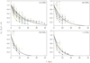 |
Fig. 5 Normalized flux-density radial profiles along the stripped tails. Each solid line and markers correspond to an individual galaxy in the sample. Line colours for individual galaxies are consistent across the four panels. The dashed line in each panel shows the best-fit exponential decline for each frequency band. |
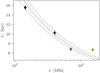 |
Fig. 6 Exponential scale length as a function of frequency for the radial profiles shown in Fig. 5. The solid and dashed lines shows the best-fit model of square-root decline and its 1σ confidence interval. Such a decline is the expectation for the very simple scenario of constant stripping velocity in a uniform magnetic field (see the main text for details). |
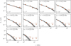 |
Fig. 7 Radio continuum spectra and best-fit ageing model along the stripped tail of MRK0057. Data points show observed flux densities, and the solid black line shows the best-fit (median) ageing model along with the 84, 95, and 99.7% credible regions (shading). Error bars on flux densities are determined following the procedure outlined in Sect. 3, and error bars on the frequency axis correspond to the bandwidth of the observing band. If significant (>3σ) flux density is not detected in an aperture, we show 3σ upper limits. We list the best-fit break frequency (vb) as well as the distance along the stripped tail (ℓ) in each panel. |
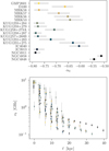 |
Fig. 9 Best-fit parameters from the ageing model fits to the stripped tails. Data points are coloured according to galaxy and are consistent between panels. Top: distribution of best-fit injection spectral indices on a galaxy-by-galaxy basis. Error bars correspond to 68% credible regions from the posterior distribution. Bottom: best-fit break frequency as a function of distance along the tail. Each marker corresponds to a single measurement for an individual galaxy, and error bars span the 68% credible region. In the ℓ = 0 bin, upper limits correspond to galaxies with purely power-law spectra and are shown at vb = 10 GHz, which is the upper limit of our prior distribution. To improve readability, in each distance bin data points are randomly shifted along the x-axis according to a Gaussian distribution with µ = 0 and σ = 0.5 kpc. |
5.3 Stripping timescales
Given that our ageing model shows broad agreement with measured tail flux-densities, we can constrain the timescales over which material is removed from these galaxies by estimating the radiative age of the plasma as a function of distance along the radio tail. The radiative age (Miley 1980) is given by
 (6)
(6)
where vb is the break frequency in MHz, z is the source redshift, B is the magnetic field in µG, and BCMB is cosmic microwave background equivalent magnetic field given by BCMB = 3.25(1 + z)2 µG. Thus, given the best-fit break frequency from our ageing model, and an assumed magnetic field strength, we can estimate a radiative age for each distance bin along the observed radio tails.
In Fig. 10 we show trad as a function of ℓ for each of the galaxies in our sample. Since we do not have constraints on the magnetic field strength in the stripped tails, we considered a range of possible values. We set the low end of this range to be the minimum energy loss magnetic field, which is given by  for the Coma Cluster; we considered an intermediate field strength of 6 µG, and a maximum field strength of 10 µG. This maximum of 10 µG is set in order to encapsulate the small number of observational estimates on field strengths in ram-pressure-stripped tails in other clusters (Müller et al. 2021: 2–4 µG, Vollmer et al. 2021: 6–7 µG, Ignesti et al. 2022b: <10 µG). Depending on the assumed magnetic field strength, we find radiative ages that increase from tens of megayears near the galaxy disc out to two or three hundred megayears at the edge of the tail.
At fixed magnetic field strength, Fig. 10 shows that a linear relationship between trad and ℓ is a good descriptor for all galaxies in our sample. This is consistent with the commonly made assumption that CRE transport in ram-pressure-stripped tails is dominated by advection. As a result of this, we determined the slope of best-fit linear trend between trad and ℓ in order to estimate a constant bulk velocity for the plasma being stripped along the tail. The data points and best-fit trends in Fig. 10 are then coloured according to this bulk velocity. Roughly speaking, the best-fit velocities are of the order of hundreds of kilometres per second. The specific values for each galaxy and magnetic field assumption are listed in Table 3. We stress that these are projected velocities, since ℓ is projected on the sky, and therefore must be lower limits on the 3D stripping speed.
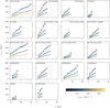 |
Fig. 10 Radiative age versus projected distance along the tail for each of the galaxies in our sample. For each distance bin we plot three estimates of radiative age, corresponding to assumed magnetic field strengths of 1.96 (minimum-loss field), 6, and 10 µG. The radiative age increases monotonically with decreasing magnetic field strength. For each assumed magnetic field strength, we show the best-fit linear relationship between the radiative age and the distance along the tail, which gives an estimate for the projected bulk velocity of cosmic rays along the tail. Data markers and best-fit lines are coloured according to the best-fit projected velocity. |
Stripped plasma velocity estimates.
6 Discussion
6.1 Radio continuum properties in the discs of ram-pressure-stripped galaxies
The first part of the analysis in this work is focused on probing the spectral properties of radio continuum emission within the discs of the ram-pressure-stripped galaxies in our sample. While ram pressure is oft associated with tails of stripped debris (e.g. jellyfish galaxies), it also can significantly alter the conditions of both the thermal and non-thermal ISM within the disc. For example, through outside-in quenching (e.g. Cortese et al. 2012; Schaefer et al. 2017, 2019; Yoon et al. 2017), gas compression (e.g. Cramer et al. 2020; Troncoso-Iribarren et al. 2020; Roberts et al. 2022a), localized starbursts (e.g. Gavazzi et al. 2001; Tomičić et al. 2018; Boselli et al. 2021; Hess et al. 2022; Roberts et al. 2022a,c), magnetic field strength amplification (e.g. Gavazzi & Boselli 1999; Murphy et al. 2009; Vollmer et al. 2013; Chen et al. 2020), etc. All of these examples can be constrained, to some extent, with multi-frequency radio continuum observations like those in this work.
Many previous works have found evidence for enhanced star formation in galaxies undergoing ram pressure stripping (e.g. Ebeling et al. 2014; Poggianti et al. 2016; Vulcani et al. 2018; Roberts & Parker 2020; Wang et al. 2020; Roberts et al. 2021a).
This is thought to be a product of the external pressure both increasing molecular gas densities and increasing the efficiency with which atomic gas in converted to the molecular form, which in both cases can lead to an increase in star formation prior to gas depletion (e.g. Bothun & Dressler 1986; Gavazzi et al. 2001; Merluzzi et al. 2013; Lee et al. 2017; Cramer et al. 2020; Troncoso-Iribarren et al. 2020; Moretti et al. 2020a,b; Boselli et al. 2021; Hess et al. 2022; Roberts et al. 2022a, 2023). One can then ask, for this scenario, what is the expected effect on radio continuum emission. In principle, the increased ISM densities should lead to increased ionization losses and thus a flattening of the low-frequency spectral index (e.g. Basu et al. 2015; Chyży et al. 2018). This has previously been invoked to explain flat spectral indices at low frequencies for galaxies undergoing ram pressure stripping (Ignesti et al. 2022b; Roberts et al. 2022c). In this work we find tentative evidence for this flattening. In the colour-colour plot in Fig. 2, the median low-frequency spectral index is marginally flatter than the high-frequency spectral index. Furthermore, there are a handful of galaxies with αlow,disc > αhigh,disc at > 2σ significance, but no galaxies with αlow,disc < αhigh,disc at the same significance level. Ultimately this is still unconvincing in a statistical sense in this work, and a wider range in frequency is necessary for stronger constraints to be possible. This should include both higher- (e.g. 5 GHz) and lower-frequency (50 MHz; LOFAR LBA) data in order to extend the lever arm in both directions.
The spectral index maps in Fig. 3 also support such a scenario. For a majority of galaxies in the sample, the flattest spectral indices are found on the leading half, opposite to the tail direction (Fig. 4). The leading half is the site that should be associated with the strongest gas compression, though it is also subject to shocks are driven into the ISM by ram pressure at the galaxy – ICM interface (Vollmer et al. 2004; Murphy et al. 2009; Pedrini et al. 2022). Such an offset between the galaxy centre and the location of the flattest spectrum for a galaxy undergoing ram pressure stripping was first noted by Vollmer et al. (2004) for NGC4522 in the Virgo Cluster. Vollmer et al. (2004) suggested that this is a signature of a ram-pressure-induced shock, which accelerates CREs and in turn leads to a flat spectral index. This is corroborated by a ridge of polarized emission on the leading edge of NGC4522, which would not be expected from the turbulent motions associated with star formation. It is possible, if not likely, that a combination of gas compression and/or star formation and shocks is contributing to the observed flat spectral indices on the leading halves of the galaxies in this work. Roberts et al. (2022a) have shown that many of the galaxies in this sample do show evidence for enhanced star formation on their leading halves. Moving forwards, observations of polarized radio flux for this sample will help in determining whether similar ridges of polarized emission are present for ram-pressure-stripped galaxies in Coma, as have been seen for similar types of galaxies in the Virgo Cluster (Vollmer et al. 2004, 2010, 2013; Chyży et al. 2007; Murphy et al. 2009).
6.2 Spectral ageing along the stripped tails
For the ram pressure tails considered in this work, the decline in flux density with increasing distance from the galaxy is broadly consistent with a simple model of synchrotron ageing. This is generally true for all four frequencies, though there are some hints of deviations at 1.5 GHz (but this is also the frequency band with the fewest detections in the tails). This is consistent with previous studies where it is argued that these stripped tails visible in the radio continuum are formed from CREs that are accelerated by star formation in the galaxy disc, and subsequently removed from the galaxy by ram pressure (e.g. Chen et al. 2020; Roberts et al. 2021a). In the absence of newly injected CREs or re-acceleration, this framework will lead to steeper spectral indices in the stripped tails than the galaxy discs (assuming that the disc is actively star forming). This has been previously confirmed for a relatively small number of galaxies (Vollmer et al. 2004; Chen et al. 2020; Müller et al. 2021; Ignesti et al. 2022b, 2023; Roberts et al. 2022c; Venturi et al. 2022), and here we show that it holds for a relatively large set of ram-pressure-stripped galaxies in Coma (Fig. 2). The steep spectral indices imply that low-frequency imaging is particularly useful for identifying galaxies with ram pressure tails in low-z groups and clusters, as evidenced by the large number of such tailed sources identified by Roberts et al. (2021a) compared to surveys at higher frequencies (e.g. Miller et al. 2009a; Chen et al. 2020).
The dominant mode of CRE transport in forming ram-pressure-stripped tails is believed to be advection/streaming (Murphy et al. 2009; Vollmer et al. 2013; Müller et al. 2021; Ignesti et al. 2022a). We estimate a constant streaming velocity (trad ∝ ℓ) for each galaxy in Fig. 10. While our estimates on the bulk velocity cover a relatively broad range due to the uncertainty in the magnetic field strength, they are consistent with previous estimates in the literature that derive stripping timescales from synchrotron radiative ages. Vollmer et al. (2021) estimate a bulk velocity limit of ≳140 km s−1 based on 1.4 and 5 GHz observations of the Virgo galaxy NGC 4330. Ignesti et al. (2023) have published estimates for plasma velocities in the ram-pressure-stripped tails of galaxies in the cluster Abell 2255. For five galaxies with monotonically decreasing flux-density profiles, Ignesti et al. (2023) constrain the projected bulk velocity to be between 160 and 430 km s−1, based off of synchrotron cooling timescale arguments. These estimates are derived assuming a minimum-loss magnetic field, and thus formally are lower limits. Constraints from hydrodynamical simulations generally show that gas velocities during ram pressure stripping are < 1000 km s−1 (e.g. Tonnesen & Bryan 2010; Steinhauser et al. 2016; Choi et al. 2022). These gas velocity constraints can be compared to to bulk plasma velocities constrained in this work under the assumption that magnetic fields remain frozen in to the ISM during stripping, and thus that the stripped cosmic rays also track the stripped gaseous ISM.
6.3 A broad picture of the impact from ram pressure on the non-thermal ISM in Coma satellites
To conclude, we discuss a general picture of the impact from ram pressure on the radio continuum spectra of star-forming satellites, which is consistent with the observations of Coma Cluster galaxies presented in this work.
As galaxies traverse the ICM in galaxy clusters, the non-thermal ISM is both perturbed within the galaxy disc and stripped off of the galaxy to form a radio tail. The formation of the radio tail can also be aided by the presence of ICM magnetic field accreted onto the galaxy via magnetic draping (Dursi 6 Pfrommer 2008; Pfrommer & Dursi 2010; Müller et al. 2021). In clusters, this typically occurs on first infall towards orbital pericentre (Roberts et al. 2021a; Smith et al. 2022). For a snapshot in time, the fraction of star-forming cluster galaxies (at low-z) with stripped radio tails is roughly 20 per cent (Roberts et al. 2021b), though this figure does not include those galaxies that may have been previously tailed and are now sufficiently stripped, nor those galaxies in a pre-stripping phase that may develop a tail in the future. It may be that most, or all, star-forming galaxies in clusters form a radio tail, but this remains an open question.
Perturbations within the disc manifest themselves in the synchrotron spectral index – both in a resolved and integrated sense. Perturbations are strongest on the leading half of the disc where the spectral index becomes flattest. In some cases the spectral index becomes flatter than the typical expected range for star formation (Fig. 3; see also Ignesti et al. 2022b; Roberts et al. 2022c). This could be a result of increased ionization losses related to compression of the ISM by the external ram pressure (e.g. Moretti et al. 2020b,a, 2023; Troncoso-Iribarren et al. 2020; Ignesti et al. 2022b; Roberts et al. 2022c,a, 2023). Magnetic field lines should also be compressed in the disc by ram pressure, which may contribute to the unusually high radio luminosity to SFR ratios in cluster galaxies – particularly those with ram-pressure-stripped tails (e.g. Gavazzi & Boselli 1999; Murphy et al. 2009; Vollmer et al. 2013; Chen et al. 2020). Ridges of polarized emission have also been observed along the leading edge of ram-pressure-stripped galaxies (e.g. Vollmer et al. 2004; Vollmer & Huchtmeier 2007; Chyży et al. 2007), a further signature of the interaction at the ISM – ICM interface, and that may indicate that CRE acceleration from shocks is also playing a role in the observed flat spectral indices.
In many cases the distribution of synchrotron emission becomes truncated, particularly on the leading half, due to the outside-in removal of CREs from the disc. Through this truncation, CREs are transported, likely through advection (e.g. Murphy et al. 2009; Vollmer et al. 2013; Ignesti et al. 2022a), from the disc downstream along the stripped tail. As CREs move further along the tail, their spectra age through synchrotron and inverse-Compton losses, leading to a decrease in radio flux density and curvature in the spectrum. This ageing along the tail is consistent with a relatively constant projected stripping velocity, of the order of hundreds of kilometres per second. Observational estimates of this stripping velocity is highly dependent on the assumed magnetic field strength, which is very poorly constrained observationally. Most galaxies show no evidence for fresh injection of CREs or re-acceleration in the stripped tail, suggesting that any radio flux density produced by extra-planar star formation in the tail is subdominant to that from the ageing plasma stripped off of the disc. This is consistent with the low SFRs observed in ram-pressure-stripped tails (e.g. Sun et al. 2007; Hester et al. 2010; Fumagalli et al. 2011; Vulcani et al. 2018; Poggianti et al. 2019; Junais et al. 2021). For example, a typical extra-planar HII region with a SFR of 10−3 M⊙ yr−1 will only produce a 1.5 GHz flux density of ~1 µJy (at the distance of Coma).
The framework outlined above is consistent with the observations of ram-pressure-stripped galaxies in Coma presented here. Future observations of polarized intensity for these galaxies would provide a further test of its consistency. Constraining the applicability of this picture beyond requires both the identification of a significant number of ram-pressure-stripped galaxies in another (likely nearby) cluster and multi-frequency radio continuum observations of said galaxies. The stripped tails of jellyfish galaxies in Abell 2255 are broadly consistent with this picture (Ignesti et al. 2023), and moving forwards, the Virgo Cluster is another obvious testing ground where significant work has already been done at high frequencies (e.g. Crowl et al. 2005; Chyży et al. 2007; Murphy et al. 2009; Vollmer et al. 2004, 2010, 2013). With recent low-frequency data (see the VICTORIA project, Edler et al. 2023), direct comparisons between galaxies in Virgo and this work can be made.
7 Conclusions
In this work we have presented a comprehensive radio continuum study of 25 ram-pressure-stripped satellite galaxies in the Coma Cluster. We used a nearly continuous frequency coverage between 144 MHz and 1.5 GHz to constrain radio spectral properties from galaxy discs all the way across their stripped radio tails. Below we itemize the main scientific conclusions from this work:
Spectral indices integrated over the galaxy discs cover a range between −0.8 and −0.3. Roughly half of the galaxy disc sample have integrated spectral indices that are > −0.5, that is to say, flatter than the typical value for injection by star formation (Fig. 2).
Ram-pressure-stripped tails have steep integrated spectral indices. All the tails in our sample are consistent with αtail < −1. The integrated spectral indices over the tails are clearly steeper than those measured over the disc, consistent with spectral ageing as the plasma is removed from the galaxy (Fig. 2).
Resolved spectral index maps of the discs show that the leading halves of the disc (i.e. the direction opposite to the tail direction) have systematically flatter spectral indices compared to the rest of the disc. This is consistent with a scenario in which gas is compressed by ram pressure, leading to enhanced local star formation and/or increased CRE ionization losses and/or the presence of ram-pressure-induced shocks (Figs. 3 and 4).
The scale lengths of the stripped radio tails decrease with increasing observing frequency. This decrease is roughly in proportion to the inverse square root of the frequency, which is the expectation from a simple model of constant stripped plasma velocity in a uniform magnetic field (Figs. 5 and 6).
For the vast majority of galaxies in our sample, radio continuum spectra extracted at various distances along the observed tails are well reproduced by a simple model of spectral ageing due to synchrotron and inverse-Compton losses (Figs. 7–9).
The radio tails in our sample show linear relationships between radiative age and distance along the tail, implying roughly constant (projected) bulk stripping velocities with magnitudes of the order of hundreds of kilometres per second (Fig. 10).
This work is an example of the value that can be derived from sensitive, high-resolution radio continuum observations in the context of advancing our understanding of ram pressure stripping in galaxy clusters. Moving forwards, this analysis could be furthered by homogenizing the frequency coverage for all galaxies in the sample. Specifically, this will require filling in gaps in the 700 MHz and 1.5 GHz imaging. Lower-frequency data from the LOFAR LBA will likely also become available moving forwards. An ultimate goal of broadband, multi-frequency imaging (e.g. from approximately tens of megahertz to a few gigahertz) covering the full Coma Cluster within the virial radius would allow for a complete study of the environmental impact on the non-thermal ISM in galaxies that are part of this nearest massive cluster. This is, in principle, achievable thanks to the large primary beams of radio facilities such as LOFAR, the uGMRT, the VLA, and MeerKAT (not to mention next-generation facilities) but will still require a significant observational commitment.
Acknowledgements
The authors thank William Forman for comments on a draft of the paper and his effort invested into obtaining the uGMRT data used in this work, Neal Miller for comments on a draft of the paper, and Larry Rudnick for helpful discussions on flux-density scale during the preparation of the paper. I.D.R. and R.Jv.W. acknowledge support from the ERC Starting Grant Cluster Web 804208. D.V.L. acknowledges the support of the Department of Atomic Energy, Government of India, under project no. 12-R &D-TFR-5.02-0700. M.S. acknowledges support from the NASA grant 80NSSC22K1508 and the USRA SOFIA grant 09_0221 provided by NASA. A.I. acknowledges funding from the European Research Council (ERC) under the European Union’s Horizon 2020 research and innovation programme (grant agreement No. 833824, PI Poggianti), and the INAF founding program ‘Ricerca Fondamentale 2022’ (PI: A. Ignesti). This work would not have been possible without the following software packages: AstroPy (Astropy Collaboration 2013), CASA (CASA Team 2022), ChainConsumer (Hinton 2016), CMasher (van der Velden 2020), DS9 (Joye & Mandel 2003), Emcee (Foreman-Mackey et al. 2013), Matplotlib (Hunter 2007), NumPy (Harris et al. 2020), Photutils (Bradley et al. 2022b), Regions (Bradley et al. 2022a), RSMF (https://rsmf.readthedocs.io/en/latest/source/howto.html), SciPy (Virtanen et al. 2020), Synchrofit (Turner et al. 2018; Turner 2018). This work is based in part on data collected at Subaru Telescope, which is operated by the National Astronomical Observatory of Japan. We thank the staff of the GMRT that made these observations possible. The GMRT is run by the National Centre for Radio Astrophysics of the Tata Institute of Fundamental Research. The National Radio Astronomy Observatory is a facility of the National Science Foundation operated under cooperative agreement by Associated Universities, Inc. LOFAR (van Haarlem et al. 2013) is the Low Frequency Array designed and constructed by ASTRON. It has observing, data processing, and data storage facilities in several countries, which are owned by various parties (each with their own funding sources), and which are collectively operated by the ILT foundation under a joint scientific policy. The ILT resources have benefitted from the following recent major funding sources: CNRS-INSU, Observatoire de Paris and Université d’Orléans, France; BMBF, MIWF-NRW, MPG, Germany; Science Foundation Ireland (SFI), Department of Business, Enterprise and Innovation (DBEI), Ireland; NWO, The Netherlands; The Science and Technology Facilities Council, UK; Ministry of Science and Higher Education, Poland. Funding for the NASA-Sloan Atlas has been provided by the NASA Astrophysics Data Analysis Program (08-ADP08-0072) and the NSF (AST-1211644). Funding for SDSS-III has been provided by the Alfred P. Sloan Foundation, the Participating Institutions, the National Science Foundation, and the US Department of Energy. The SDSS-III web site is http://www.sdss3.org.SDSS-III is managed by the Astrophysical Research Consortium for the Participating Institutions of the SDSS-III Collaboration including the University of Arizona, the Brazilian Participation Group, Brookhaven National Laboratory, University of Cambridge, University of Florida, the French Participation Group, the German Participation Group, the Instituto de Astrofisica de Canarias, the Michigan State/Notre Dame/JINA Participation Group, Johns Hopkins University, Lawrence Berkeley National Laboratory, Max Planck Institute for Astrophysics, New Mexico State University, New York University, Ohio State University, Pennsylvania State University, University of Portsmouth, Princeton University, the Spanish Participation Group, University of Tokyo, University of Utah, Vanderbilt University, University of Virginia, University of Washington, and Yale University.
Appendix A Deviations from the ageing model for NGC4858: A contribution from extra-planar star formation?
While the vast majority of flux-density measurements are well reproduced by the ageing model (see Fig. 8), the galaxy in the sample with the largest deviations from the ageing model predictions is NGC4858. This is visible in the spectrum plots in Fig. B.27 where two clear offsets between the model and data are visible. First, at ℓ = 0″ the model significantly under-predicts the observed 144 MHz flux density, and second, at ℓ = 14″ and ℓ = 21″ the model under-predicts the observed 1.5 GHz flux density. The S/N of the deviations at 1.5 GHz are 5.4 and 3.1, respectively. We note that there is also a flux excess in the ℓ = 35″ bin in Fig. B.27, though we believe that this is most likely a noise spike since it is detached from the rest of the 1.5 GHz tail and it does not overlap with the observed extra-planar Hα emission for NGC4858 (see below). Müller et al. (2021) present evidence for extra-planar star formation in a ram-pressure-stripped tail in the form of a flat spectral index between 1.4 and 3 GHz. It is possible that the aforementioned flux excesses at 1.5 GHz are also connected to ongoing star formation. We stress that this section is only meant to be a broad evaluation of the plausibility of this scenario. We recognize the substantial uncertainties, both in terms of the robustness of the 1.5 GHz excess outlined above and of estimating extra-planar SFRs from narrowband imaging (see below). Towards the end of this section we discuss these uncertainties more thoroughly and provide a forecast for how they can be reduced (though certainly not eliminated) moving forwards.
NGC4858 is one of the poster children in the Coma Cluster for ongoing star formation in a ram-pressure-stripped tail (Smith et al. 2010; Yagi et al. 2010). Qualitatively, extra emission from ongoing star formation could potentially explain the offsets between the data and model in Fig. B.27. Synchrotron emission from recent star formation will have a flat spectral index, and thus when superimposed with steep-spectrum, aged plasma, the relative contribution from star formation will be most apparent at the high-frequency end. Therefore, extra-planar star formation could, at least partially, account for the 1.5 GHz excess while only making a relatively small contribution at low frequencies. In this scenario, the observed tail spectrum would be a composite of an aged spectrum (e.g. a JP model) and a flat, power-law spectrum:
 (A.1)
(A.1)
where  is an aged JP model as described in Sect. 5.2,
  is the power-law flux density at 1.5 GHz, and we opted for a power-law spectral index of −0.5, which is similar to the best-fit injection index for NGC4858 (see Figs. 9 and B.58). Assuming a steeper injection index of −0.6 or −0.7 does not alter the qualitative conclusions. We then explored whether such a composite model is able to account for the observed discrepancies between the data and a solely ageing model for NGC4858.
We first re-fitted the data with the ageing model described in Sect. 5.2, but only include 144, 400, and 700 MHz flux densities in the fit, since in this scenario the 1.5 GHz flux density may be contaminated by emission from recent star formation. It is true that emission from star formation will affect flux densities at all frequencies, but again, superimposed on an aged plasma the relative impact will be largest at high frequencies (especially for vb ≲ 1 GHz), and therefore omitting the 1.5 GHz data from the fit will give a better estimate for the aged plasma component. Fig. A.1 shows the spectra along the tail for NGC4858 (same data points as Fig. B.27), but now overlaid with an ageing model fit only to the 144, 400, and 700 MHz data, not 1.5 GHz. Compared to Fig. B.27 the break frequencies are shifted to slightly lower frequencies, and the 144 MHz flux density at ℓ = 0″ is no longer a > 3σ outlier. This is a result of the ageing model not being compelled to account for the relatively large observed flux density at 1.5 GHz. For the two previously mentioned distance bins along the tail (ℓ = 14″, 21″) there is now slightly stronger evidence for excess 1.5 GHz emission with respect to the updated ageing model.
To determine the level of star formation required in the tail to account for this excess 1.5 GHz flux density, we added a power-law component to the ageing model shown in Fig. A.1 and fit to the observed 144 MHz to 1.5 GHz flux densities to determine the best-fit power-law normalization at 1.5 GHz for the composite model described by Eq. A.1. This gives an estimate for the flux density at 1.5 GHz due to star formation that is required to account for the observed excess. We used the SFR − L1.5 calibration from Kennicutt & Evans (2012),
 (A.2)
(A.2)
to convert this value to an expected SFR. In Fig. A.2 we show the results of this composite model fitting for the two distance bins along the tail where there is an observed 1.5 GHz excess. Fig. A.2 shows the ageing component (grey) as well as the best-fit power-law component and composite model (gold). We also list the required SFR for each distance bin derived from the best-fit normalization for the power-law component. The required SFRs are between 10−2 and 10−1 M⊙ yr−1, for a total of 0.11 ± 0.02 M⊙ yr−1. Not unprecedented, but on the high end relative to extra-planar SFRs that have been observed in other galaxies (e.g. Sun et al. 2007; Hester et al. 2010; Fumagalli et al. 2011; Vulcani et al. 2018; Cramer et al. 2019; Poggianti et al. 2019; Boselli et al. 2021; Junais et al. 2021). Because there are existing observations showing Ha emission within the stripped tail of NGC4858, we can test more directly if there is sufficient star formation in the tail to match the required SFRs listed in Fig. A.2. We note that both distance bins considered above overlap spatially with the observed Ha tail for NGC4858 (see Yagi et al. 2010).
To constrain observed SFRs in the tail of NGC4858, we used narrowband Hα + NII imaging from Yagi et al. (2010) taken with the Subaru Suprime-Cam. The line emission was isolated by using the R band for continuum subtraction, though we note that there is significant uncertainty associated with the continuum subtraction for regions where there is strong underlying continuum emission (see Yagi et al. 2010, 2017 for a more detailed discussion), for example galaxy discs. Here we only considered extra-planar emission in the tail, where strong continuum emission is not expected, and therefore the continuum subtraction in order to isolate the line emission is relatively reliable.
We measured the narrowband flux over the tail regions and this flux is converted to a SFR assuming the calibration from Kennicutt & Evans (2012),
 (A.3)
(A.3)
We calculated SFRs for a range of assumed [NII]-to-Hα ratios, as this cannot be directly constrained from the narrowband imaging. We also considered a range in ƒSF, which we define as the fraction of Hα + NII flux originating from extraplanar star formation, as the ionization source (and therefore, loosely, fSF) cannot be constrained directly from narrowband imaging.
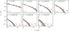 |
Fig. A.1 Radio continuum spectra and best-fit ageing model along the stripped tail of NGC4858, fit only to the 144, 400, and 700 MHz data. Panels follow the same formatting as Fig. 7. |
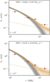 |
Fig. A.2 Radio continuum spectra for distance bins that show an excess of 1.5 GHz emission relative to the ageing model. Data points correspond to observed flux densities, grey shading corresponds to the ageing model, dashed gold line shows the best-fit power-law component, and the gold shading shows the composite ageing plus power-law model. Each panel lists the best-fit SFR required in order to reproduce the observed flux density excess at 1.5 GHz. |
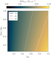 |
Fig. A.3 SFR derived from observed Hα + NII emission in the tail, for a grid of different assumed values for the [NII]-to-Hα- ratio and ƒSF. We also plot 1σ, 2σ, and 3σ contours for the ‘required’ SFRs from the composite fits shown in Fig. A.2. |
In Fig. A.3 we plot the ‘observed’ SFR, derived from the Hα + NII flux in the tail, for a grid of different assumed values for the [NII]-to-Ha ratio and fSF We also plot 1σ, 2σ, and 3σ contours corresponding to the best-fit, total SFR in the tail from the composite fits shown in Fig. A.2. It is possible to account for the best-fit SFR from the observed Hα + NII emission, within the fit uncertainties, but doing so requires both a very large value for ƒSF and a relatively low value for the [NII]-to-Hα ratio. Not impossible, but in tension with most previous constraints on these parameters (e.g. Yagi et al. 2007; Cramer et al. 2019; Poggianti et al. 2019). While it is difficult to account for the full excess 1.5 GHz emission in the tail, for NGC4858, Fig. A.3 shows that a significant portion of this excess could be explained by extraplanar star formation.
Of course, it is paramount to acknowledge the uncertainties beyond the [NII]-to-Hα ratio and ƒSF that go into Fig. A.3. These include uncertainties around internal extinction in star-forming regions in the tail, continuum subtraction in the narrowband, and likely most significant, uncertainties on the calibrations from Hα and 1.5 GHz luminosities to SFR. Not to mention the assumptions that go into the ageing model (see Sect. 5.2) that directly feed into SFRfit. Bearing all this in mind, factor of two uncertainties on the SFRs in this section are likely a minimum. Thus, while we cannot rule out the scenario where extra-planar star formation is driving the 1.5 GHz excess, a stronger statement is not possible. Forthcoming integral field unit (IFU) spectroscopy with the WEAVE Large IFU (PI Roberts) of the ~30 LoTSS jellyfish galaxies (Roberts et al. 2021a) in the Coma Cluster (including NGC4858) and their stripped tails, will alleviate some of the aforementioned uncertainties on the measured SFR in the tail. Deep radio continuum imaging at higher frequencies (e.g. 3 – 5 GHz) will also be important for confirming the existence of excess emission at high frequencies.
Appendix B Plots and images for individual galaxies
In this appendix we include images of all galaxies from our analysis with the disc and tail apertures overlaid. For galaxies that are included in the tail spectral modelling analysis, we also show plots of continuum spectra at various distances along the tail as well as corner plots showing the results of the MCMC fits.
Appendix B.1 NGC4848
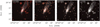 |
Fig. B.1 Radio – optical overlay images for the galaxy NGC4848. Background image is a three-colour grz image from the Legacy Surveys (Dey et al. 2019). Contour levels begin at 2.5 × rms and increase by a factor of three with each step. In the lower left we show the common FWHM beam size of 6.5″. In each panel we also overlay the galaxy disc aperture (dashed ellipse) and the apertures used to measure radio continuum flux densities along the tail (solid rectangles). |
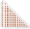 |
Fig. B.3 MCMC fitting results for the ageing model along the tail. |
Appendix B.2 NGC4853
Appendix B.3 NGC4858
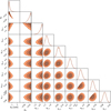 |
Fig. B.7 MCMC fitting results for the ageing model along the tail. |
Appendix B.4 NGC4911
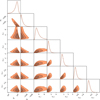 |
Fig. B.10 MCMC fitting results for the ageing model along the tail. |
Appendix B.5 IC3913
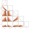 |
Fig. B.13 MCMC fitting results for the ageing model along the tail. |
Appendix B.6 IC3949
Appendix B.7 IC4040
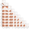 |
Fig. B.17 MCMC fitting results for the ageing model along the tail. |
Appendix B.8 KUG1250+276
Appendix B.9 KUG 1255+275
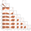 |
Fig. B.21 MCMC fitting results for the ageing model along the tail. |
Appendix B.10 KUG1255+283
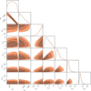 |
Fig. B.24 MCMC fitting results for the ageing model along the tail. |
Appendix B.11 KUG1256+287B
Appendix B.12 KUG1257+288B
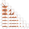 |
Fig. B.28 MCMC fitting results for the ageing model along the tail. |
Appendix B.13 KUG1258+279A
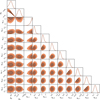 |
Fig. B.31 MCMC fitting results for the ageing model along the tail. |
Appendix Β.14 KUG1258+287
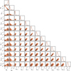 |
Fig. B.34 MCMC fitting results for the ageing model along the tail. |
Appendix Β.15 KUG1259+279
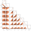 |
Fig. B.37 MCMC fitting results for the ageing model along the tail. |
Appendix Β.16 KUG1259+284
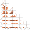 |
Fig. B.40 MCMC fitting results for the ageing model along the tail. |
Appendix B.17 MRK0053
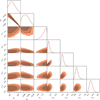 |
Fig. B.43 MCMC fitting results for the ageing model along the tail. |
Appendix B.18 MRK0056
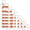 |
Fig. B.46 MCMC fitting results for the ageing model along the tail. |
Appendix B.19 MRK0057
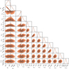 |
Fig. B.49 MCMC fitting results for the ageing model along the tail. |
Appendix B.20 MRK0058
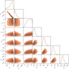 |
Fig. B.52 MCMC fitting results for the ageing model along the tail. |
Appendix B.21 D100
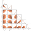 |
Fig. B.55 MCMC fitting results for the ageing model along the tail. |
Appendix B.22 GMP2601
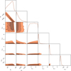 |
Fig. B.58 MCMC fitting results for the ageing model along the tail. |
Appendix B.23 GMP3618
Appendix B.24 GMP5226
References
- Astropy Collaboration (Robitaille, T. P., et al.) 2013, A&A, 558, A33 [NASA ADS] [CrossRef] [EDP Sciences] [Google Scholar]
- Balogh, M. L., Navarro, J. F., & Morris, S. L. 2000, ApJ, 540, 113 [Google Scholar]
- Basu, A., Beck, R., Schmidt, P., & Roy, S. 2015, MNRAS, 449, 3879 [NASA ADS] [CrossRef] [Google Scholar]
- Bell, A. R. 1978, MNRAS, 182, 147 [Google Scholar]
- Biermann, P. L., & Strom, R. G. 1993, A&A, 275, 659 [NASA ADS] [Google Scholar]
- Bigiel, F., Leroy, A. K., Walter, F., et al. 2011, ApJ, 730, L13 [NASA ADS] [CrossRef] [Google Scholar]
- Bogdan, T. J., & Volk, H. J. 1983, A&A, 122, 129 [NASA ADS] [Google Scholar]
- Bonafede, A., Brunetti, G., Rudnick, L., et al. 2022, ApJ, 933, 218 [NASA ADS] [CrossRef] [Google Scholar]
- Boselli, A., Fossati, M., Ferrarese, L., et al. 2018, A&A, 614, A56 [NASA ADS] [CrossRef] [EDP Sciences] [Google Scholar]
- Boselli, A., Lupi, A., Epinat, B., et al. 2021, A&A, 646, A139 [NASA ADS] [CrossRef] [EDP Sciences] [Google Scholar]
- Boselli, A., Fossati, M., & Sun, M. 2022, A&ARv, 30, 3 [NASA ADS] [CrossRef] [Google Scholar]
- Bothun, G. D., & Dressler, A. 1986, ApJ, 301, 57 [NASA ADS] [CrossRef] [Google Scholar]
- Bradley, L., Deil, C., Patra, S., et al. 2022a, https://zenodo.org/records/7259631 [Google Scholar]
- Bradley, L., Sipocz, B., Robitaille, T., et al. 2022b, https://zenodo.org/records/6825892 [Google Scholar]
- Bravo-Alfaro, H., Cayatte, V., van Gorkom, J. H., & Balkowski, C. 2000, AJ, 119, 580 [Google Scholar]
- Briggs, D. S. 1995, AAS Meeting Abstracts, 187, 112.02 [Google Scholar]
- Brown, T., Roberts, I. D., Thorp, M., et al. 2023, ApJ, 956, 37 [NASA ADS] [CrossRef] [Google Scholar]
- CASA Team, Bean, B., Bhatnagar, S., et al. 2022, PASP, 134, 114501 [NASA ADS] [CrossRef] [Google Scholar]
- Chen, H., Sun, M., Yagi, M., et al. 2020, MNRAS, 496, 4654 [CrossRef] [Google Scholar]
- Choi, W., Kim, C.-G., & Chung, A. 2022, ApJ, 936, 133 [NASA ADS] [CrossRef] [Google Scholar]
- Chung, A., van Gorkom, J. H., Kenney, J. D. P., & Vollmer, B. 2007, ApJ, 659, L115 [Google Scholar]
- Chyży, K. T., Ehle, M., & Beck, R. 2007, A&A, 474, 415 [NASA ADS] [CrossRef] [EDP Sciences] [Google Scholar]
- Chyży, K. T., Jurusik, W., Piotrowska, J., et al. 2018, A&A, 619, A36 [NASA ADS] [CrossRef] [EDP Sciences] [Google Scholar]
- Condon, J. J. 1992, ARA&A, 30, 575 [Google Scholar]
- Cortese, L., Boissier, S., Boselli, A., et al. 2012, A&A, 544, A101 [NASA ADS] [CrossRef] [EDP Sciences] [Google Scholar]
- Cramer, W. J., Kenney, J. D. P., Sun, M., et al. 2019, ApJ, 870, 63 [Google Scholar]
- Cramer, W. J., Kenney, J. D. P., Cortes, J. R., et al. 2020, ApJ, 901, 95 [NASA ADS] [CrossRef] [Google Scholar]
- Cramer, W. J., Kenney, J. D. P., Tonnesen, S., et al. 2021, ApJ, 921, 22 [NASA ADS] [CrossRef] [Google Scholar]
- Crowl, H. H., Kenney, J. D. P., van Gorkom, J. H., & Vollmer, B. 2005, AJ, 130, 65 [Google Scholar]
- Dey, A., Schlegel, D. J., Lang, D., et al. 2019, AJ, 157, 168 [Google Scholar]
- Donas, J., Milliard, B., & Laget, M. 1995, A&A, 303, 661 [NASA ADS] [Google Scholar]
- Durret, F., Chiche, S., Lobo, C., & Jauzac, M. 2021, A&A, 648, A63 [NASA ADS] [CrossRef] [EDP Sciences] [Google Scholar]
- Dursi, L. J., & Pfrommer, C. 2008, ApJ, 677, 993 [NASA ADS] [CrossRef] [Google Scholar]
- Ebeling, H., Stephenson, L. N., & Edge, A. C. 2014, ApJ, 781, L40 [Google Scholar]
- Edler, H. W., de Gasperin, F., Shimwell, T. W., et al. 2023, A&A, 676, A24 [NASA ADS] [CrossRef] [EDP Sciences] [Google Scholar]
- Edwards, L. O. V., & Fadda, D. 2011, AJ, 142, 148 [NASA ADS] [CrossRef] [Google Scholar]
- Foreman-Mackey, D., Hogg, D. W., Lang, D., & Goodman, J. 2013, PASP, 125, 306 [Google Scholar]
- Fumagalli, M., Gavazzi, G., Scaramella, R., & Franzetti, P. 2011, A&A, 528, A46 [NASA ADS] [CrossRef] [EDP Sciences] [Google Scholar]
- Gavazzi, G. 1978, A&A, 69, 355 [NASA ADS] [Google Scholar]
- Gavazzi, G. 1987, ApJ, 320, 96 [NASA ADS] [CrossRef] [Google Scholar]
- Gavazzi, G. 1989, ApJ, 346, 59 [NASA ADS] [CrossRef] [Google Scholar]
- Gavazzi, G., & Boselli, A. 1999, A&A, 343, 93 [NASA ADS] [Google Scholar]
- Gavazzi, G., & Jaffe, W. 1987, A&A, 186, L1 [NASA ADS] [Google Scholar]
- Gavazzi, G., Boselli, A., Mayer, L., et al. 2001, ApJ, 563, L23 [Google Scholar]
- Gavazzi, G., Consolandi, G., Gutierrez, M. L., Boselli, A., & Yoshida, M. 2018, A&A, 618, A130 [NASA ADS] [CrossRef] [EDP Sciences] [Google Scholar]
- Ge, C., Sun, M., Liu, R.-Y., et al. 2019, MNRAS, 486, L36 [NASA ADS] [CrossRef] [Google Scholar]
- Godwin, J. G., Metcalfe, N., & Peach, J. V. 1983, MNRAS, 202, 113 [NASA ADS] [CrossRef] [Google Scholar]
- Gregg, M. D., Holden, B. P., & West, M. J. 2003, arXiv e-prints [arXiv:astro-ph/8381459] [Google Scholar]
- Gunn, J. E., & Gott, J. R. III, 1972, ApJ, 176, 1 [NASA ADS] [CrossRef] [Google Scholar]
- Hales, S. E. G., Riley, J. M., Waldram, E. M., Warner, P. J., & Baldwin, J. E. 2007, MNRAS, 382, 1639 [NASA ADS] [Google Scholar]
- Harris, C. R., Millman, K. J., van der Walt, S. J., et al. 2020, Nature, 585, 357 [NASA ADS] [CrossRef] [Google Scholar]
- Heesen, V., Staffehl, M., Basu, A., et al. 2022, A&A, 664, A83 [NASA ADS] [CrossRef] [EDP Sciences] [Google Scholar]
- Hess, K. M., Kotulla, R., Chen, H., et al. 2022, A&A, 668, A184 [NASA ADS] [CrossRef] [EDP Sciences] [Google Scholar]
- Hester, J. A., Seibert, M., Neill, J. D., et al. 2010, ApJ, 716, L14 [Google Scholar]
- Hinton, S. R. 2016, J. Open Source Softw., 1, 00045 [NASA ADS] [CrossRef] [Google Scholar]
- Ho, M., Ntampaka, M., Rau, M. M., et al. 2022, Nat. Astron., 6, 936 [NASA ADS] [CrossRef] [Google Scholar]
- Hunter, J. D. 2007, Comput. Sci. Eng., 9, 90 [NASA ADS] [CrossRef] [Google Scholar]
- Ignesti, A., Vulcani, B., Poggianti, B. M., et al. 2022a, ApJ, 937, 58 [NASA ADS] [CrossRef] [Google Scholar]
- Ignesti, A., Vulcani, B., Poggianti, B. M., et al. 2022b, ApJ, 924, 64 [NASA ADS] [CrossRef] [Google Scholar]
- Ignesti, A., Vulcani, B., Botteon, A., et al. 2023, A&A, 675, A118 [NASA ADS] [CrossRef] [EDP Sciences] [Google Scholar]
- Intema, H. T., van der Tol, S., Cotton, W. D., et al. 2009, A&A, 501, 1185 [NASA ADS] [CrossRef] [EDP Sciences] [Google Scholar]
- Jaffe, W. J., & Perola, G. C. 1973, A&A, 26, 423 [NASA ADS] [Google Scholar]
- Joye, W. A., & Mandel, E. 2003, ASP Conf. Ser., 295, 489 [Google Scholar]
- Junais, Boissier, S., Boselli, A., et al. 2021, A&A, 650, A99 [NASA ADS] [CrossRef] [EDP Sciences] [Google Scholar]
- Kenney, J. D. P., van Gorkom, J. H., & Vollmer, B. 2004, AJ, 127, 3361 [Google Scholar]
- Kennicutt, R. C., Jr. 1998, ApJ, 498, 541 [Google Scholar]
- Kennicutt, R. C., & Evans, N. J. 2012, ARA&A, 50, 531 [NASA ADS] [CrossRef] [Google Scholar]
- Lal, D. V. 2020, ApJS, 250, 22 [NASA ADS] [CrossRef] [Google Scholar]
- Lal, D. V., Lyskova, N., Zhang, C., et al. 2022, ApJ, 934, 170 [NASA ADS] [CrossRef] [Google Scholar]
- Larson, R. B., Tinsley, B. M., & Caldwell, C. N. 1980, ApJ, 237, 692 [Google Scholar]
- Lee, B., Chung, A., Tonnesen, S., et al. 2017, MNRAS, 466, 1382 [NASA ADS] [CrossRef] [Google Scholar]
- Lee, J. H., Lee, M. G., Mun, J. Y., Cho, B. S., & Kang, J. 2022, ApJ, 931, L22 [NASA ADS] [CrossRef] [Google Scholar]
- Longair, M. S. 2011, High Energy Astrophysics (Cambridge: Cambridge University Press) [Google Scholar]
- Mahajan, S., Haines, C. P., & Raychaudhury, S. 2010, MNRAS, 404, 1745 [NASA ADS] [Google Scholar]
- McPartland, C., Ebeling, H., Roediger, E., & Blumenthal, K. 2016, MNRAS, 455, 2994 [Google Scholar]
- Merluzzi, P., Busarello, G., Dopita, M. A., et al. 2013, MNRAS, 429, 1747 [Google Scholar]
- Merluzzi, P., Busarello, G., Dopita, M. A., et al. 2016, MNRAS, 460, 3345 [NASA ADS] [CrossRef] [Google Scholar]
- Miley, G. 1980, ARA&A, 18, 165 [Google Scholar]
- Miller, N. A., Hornschemeier, A. E., & Mobasher, B. 2009a, AJ, 137, 4436 [NASA ADS] [CrossRef] [Google Scholar]
- Miller, N. A., Hornschemeier, A. E., Mobasher, B., et al. 2009b, AJ, 137, 4450 [NASA ADS] [CrossRef] [Google Scholar]
- Molnár, D. C., Serra, P., van der Hulst, T., et al. 2022, A&A, 659, A94 [NASA ADS] [CrossRef] [EDP Sciences] [Google Scholar]
- Moretti, A., Paladino, R., Poggianti, B. M., et al. 2020a, ApJ, 897, L30 [Google Scholar]
- Moretti, A., Paladino, R., Poggianti, B. M., et al. 2020b, ApJ, 889, 9 [Google Scholar]
- Moretti, A., Serra, P., Bacchini, C., et al. 2023, ApJ, 955, 153 [NASA ADS] [CrossRef] [Google Scholar]
- Müller, A., Poggianti, B. M., Pfrommer, C., et al. 2021, Nat. Astron., 5, 159 [Google Scholar]
- Murphy, E. J., Kenney, J. D. P., Helou, G., Chung, A., & Howell, J. H. 2009, ApJ, 694, 1435 [CrossRef] [Google Scholar]
- Niklas, S., Klein, U., & Wielebinski, R. 1997, A&A, 322, 19 [NASA ADS] [Google Scholar]
- Offringa, A. R., McKinley, B., Hurley-Walker, N., et al. 2014, MNRAS, 444, 606 [Google Scholar]
- Pedrini, A., Fossati, M., Gavazzi, G., et al. 2022, MNRAS, 511, 5180 [NASA ADS] [CrossRef] [Google Scholar]
- Peng, Y., Maiolino, R., & Cochrane, R. 2015, Nature, 521, 192 [Google Scholar]
- Pfrommer, C., & Dursi, J. 2010, Nat. Phys., 6, 520 [NASA ADS] [CrossRef] [Google Scholar]
- Poggianti, B. M., Bridges, T. J., Komiyama, Y., et al. 2004, ApJ, 601, 197 [NASA ADS] [CrossRef] [Google Scholar]
- Poggianti, B. M., Fasano, G., Omizzolo, A., et al. 2016, AJ, 151, 78 [Google Scholar]
- Poggianti, B. M., Moretti, A., Gullieuszik, M., et al. 2017, ApJ, 844, 48 [Google Scholar]
- Poggianti, B. M., Gullieuszik, M., Tonnesen, S., et al. 2019, MNRAS, 482, 4466 [Google Scholar]
- Rines, K. J., Geller, M. J., Diaferio, A., & Hwang, H. S. 2016, ApJ, 819, 63 [NASA ADS] [CrossRef] [Google Scholar]
- Roberts, I. D., & Parker, L. C. 2020, MNRAS, 495, 554 [NASA ADS] [CrossRef] [Google Scholar]
- Roberts, I. D., van Weeren, R. J., McGee, S. L., et al. 2021a, A&A, 650, A111 [NASA ADS] [CrossRef] [EDP Sciences] [Google Scholar]
- Roberts, I. D., van Weeren, R. J., McGee, S. L., et al. 2021b, A&A, 652, A153 [NASA ADS] [CrossRef] [EDP Sciences] [Google Scholar]
- Roberts, I. D., Lang, M., Trotsenko, D., et al. 2022a, ApJ, 941, 77 [NASA ADS] [CrossRef] [Google Scholar]
- Roberts, I. D., Parker, L. C., Gwyn, S., et al. 2022b, MNRAS, 509, 1342 [Google Scholar]
- Roberts, I. D., van Weeren, R. J., Timmerman, R., et al. 2022c, A&A, 658, A44 [NASA ADS] [CrossRef] [EDP Sciences] [Google Scholar]
- Roberts, I. D., Brown, T., Zabel, N., et al. 2023, A&A, 675, A78 [NASA ADS] [CrossRef] [EDP Sciences] [Google Scholar]
- Saintonge, A., Catinella, B., Tacconi, L. J., et al. 2017, ApJS, 233, 22 [Google Scholar]
- Salim, S., Lee, J. C., Janowiecki, S., et al. 2016, ApJS, 227, 2 [NASA ADS] [CrossRef] [Google Scholar]
- Salim, S., Boquien, M., & Lee, J. C. 2018, ApJ, 859, 11 [Google Scholar]
- Sawicki, M. 2012, PASP, 124, 1208 [NASA ADS] [CrossRef] [Google Scholar]
- Schaefer, A. L., Croom, S. M., Allen, J. T., et al. 2017, MNRAS, 464, 121 [NASA ADS] [CrossRef] [Google Scholar]
- Schaefer, A. L., Croom, S. M., Scott, N., et al. 2019, MNRAS, 483, 2851 [NASA ADS] [CrossRef] [Google Scholar]
- Schmidt, M. 1959, ApJ, 129, 243 [NASA ADS] [CrossRef] [Google Scholar]
- Shapley, H. 1934, Harvard College Observ. Bull., 896, 3 [NASA ADS] [Google Scholar]
- Shimwell, T. W., Röttgering, H. J. A., Best, P. N., et al. 2017, A&A, 598, A104 [NASA ADS] [CrossRef] [EDP Sciences] [Google Scholar]
- Shimwell, T. W., Tasse, C., Hardcastle, M. J., et al. 2019, A&A, 622, A1 [NASA ADS] [CrossRef] [EDP Sciences] [Google Scholar]
- Shimwell, T. W., Hardcastle, M. J., Tasse, C., et al. 2022, A&A, 659, A1 [NASA ADS] [CrossRef] [EDP Sciences] [Google Scholar]
- Shostak, G. S., Hummel, E., Shaver, P. A., van der Hulst, J. M., & van der Kruit, P. C. 1982, A&A, 115, 293 [NASA ADS] [Google Scholar]
- Smith, R. J., Lucey, J. R., Hammer, D., et al. 2010, MNRAS, 408, 1417 [Google Scholar]
- Smith, R. J., Lucey, J. R., Price, J., Hudson, M. J., & Phillipps, S. 2012, MNRAS, 419, 3167 [NASA ADS] [CrossRef] [Google Scholar]
- Smith, R., Shinn, J.-H., Tonnesen, S., et al. 2022, ApJ, 934, 86 [NASA ADS] [CrossRef] [Google Scholar]
- Steinhauser, D., Schindler, S., & Springel, V. 2016, A&A, 591, A51 [NASA ADS] [CrossRef] [EDP Sciences] [Google Scholar]
- Sun, M., Donahue, M., & Voit, G. M. 2007, ApJ, 671, 190 [Google Scholar]
- Tabatabaei, F. S., Schinnerer, E., Krause, M., et al. 2017, ApJ, 836, 185 [Google Scholar]
- Tasse, C., Hugo, B., Mirmont, M., et al. 2018, A&A, 611, A87 [NASA ADS] [CrossRef] [EDP Sciences] [Google Scholar]
- Terlevich, A. I., Caldwell, N., & Bower, R. G. 2001, MNRAS, 326, 1547 [NASA ADS] [CrossRef] [Google Scholar]
- Tomičić, N., Hughes, A., Kreckel, K., et al. 2018, ApJ, 869, L38 [CrossRef] [Google Scholar]
- Tonnesen, S., & Bryan, G. L. 2010, ApJ, 709, 1203 [NASA ADS] [CrossRef] [Google Scholar]
- Troncoso-Iribarren, P., Padilla, N., Santander, C., et al. 2020, MNRAS, 497, 4145 [Google Scholar]
- Turner, R. J. 2018, MNRAS, 476, 2522 [CrossRef] [Google Scholar]
- Turner, R. J., Shabala, S. S., & Krause, M. G. H. 2018, MNRAS, 474, 3361 [NASA ADS] [CrossRef] [Google Scholar]
- van der Velden, E. 2020, J. Open Source Softw., 5, 2004 [Google Scholar]
- van Haarlem, M. P., Wise, M. W., Gunst, A. W., et al. 2013, A&A, 556, A2 [NASA ADS] [CrossRef] [EDP Sciences] [Google Scholar]
- Venturi, T., Giacintucci, S., Merluzzi, P., et al. 2022, A&A, 660, A81 [NASA ADS] [CrossRef] [EDP Sciences] [Google Scholar]
- Virtanen, P., Gommers, R., Oliphant, T. E., et al. 2020, Nat. Meth., 17, 261 [Google Scholar]
- Vollmer, B., & Huchtmeier, W. 2007, A&A, 462, 93 [NASA ADS] [CrossRef] [EDP Sciences] [Google Scholar]
- Vollmer, B., Beck, R., Kenney, J. D. P., & van Gorkom, J. H. 2004, AJ, 127, 3375 [NASA ADS] [CrossRef] [Google Scholar]
- Vollmer, B., Soida, M., Chung, A., et al. 2010, A&A, 512, A36 [NASA ADS] [CrossRef] [EDP Sciences] [Google Scholar]
- Vollmer, B., Soida, M., Beck, R., et al. 2013, A&A, 553, A116 [NASA ADS] [CrossRef] [EDP Sciences] [Google Scholar]
- Vollmer, B., Fossati, M., Boselli, A., et al. 2021, A&A, 645, A121 [EDP Sciences] [Google Scholar]
- Vulcani, B., Poggianti, B. M., Gullieuszik, M., et al. 2018, ApJ, 866, L25 [Google Scholar]
- Vulcani, B., Poggianti, B. M., Tonnesen, S., et al. 2020, ApJ, 899, 98 [Google Scholar]
- Vulcani, B., Poggianti, B. M., Smith, R., et al. 2022, ApJ, 927, 91 [NASA ADS] [CrossRef] [Google Scholar]
- Wang, J., Xu, W., Lee, B., et al. 2020, ApJ, 903, 103 [NASA ADS] [CrossRef] [Google Scholar]
- Yagi, M., Komiyama, Y., Yoshida, M., et al. 2007, ApJ, 660, 1209 [Google Scholar]
- Yagi, M., Yoshida, M., Komiyama, Y., et al. 2010, AJ, 140, 1814 [Google Scholar]
- Yagi, M., Yoshida, M., Gavazzi, G., et al. 2017, ApJ, 839, 65 [NASA ADS] [CrossRef] [Google Scholar]
- Yoon, H., Chung, A., Smith, R., & Jaffé, Y. L. 2017, ApJ, 838, 81 [Google Scholar]
- Zhu, J., Tonnesen, S., & Bryan, G. L. 2024, ApJ, 960, 54 [NASA ADS] [CrossRef] [Google Scholar]
All Tables
All Figures
|
Fig. 1 One-sigma sensitivity (rms) as a function of frequency for each of the observing bands in this work. All values are measured from images at our working resolution of 6.5″. Data points correspond to the local rms measured around each galaxy. For the L band, the filled markers correspond to galaxies that are covered by the Chen et al. (2020) observations and the open markers correspond to galaxies only covered by the Miller et al. (2009a) observations. Shaded bands correspond to the width of each observing band. For reference, we plot lines corresponding to spectral indices of −0.5, −1, and −1.5 anchored to the lowest-frequency band. |
| In the text | |
|
Fig. 2 Integrated spectral index measurements. Top: tail spectral index versus galaxy disc spectral index. When emission is detected in three or more frequency bands, the spectral index and its error are determined from orthogonal distance regression fits. When emission is only detected in two frequency bands, the spectral index and its error are determined via the direct method (Eq. (1)). For galaxies where emission in the tail is only detected at one frequency (see Table 2), αtail is shown as a 3σ upper limit. Bottom: radio colour-colour diagram for the galaxy discs. The high-frequency spectral index (y-axis) is measured between 700 MHz and 1.5 GHz, and the low-frequency spectral index (x-axis) is measured between 144 and 400 MHz. In both the top and bottom panels, the dashed lines correspond to the one-to-one relation. |
| In the text | |
|
Fig. 3 Spectral index maps for each galaxy disc in our sample. Spectral indices are measured between 144 MHz and νmax, as listed in each figure panel. The dashed ellipse in each panel corresponds to the r-band Petrosian 90% radius, the ‘x’ marks the optical galaxy centre, and the filled circle shows the 6.5″ beam FWHM. In the lower right of each panel, we show an arrow that points in the projected direction of the stripped tail. The typical uncertainties on the spectral index maps are ~0.05 between 144 MHz and 1.5 GHz, ~0.07 between 144 and 700 MHz, and ~0.11 between 144 and 400 MHz. |
| In the text | |
|
Fig. 4 Location of the peak (i.e. flattest) spectral index within each disc, relative to the direction of the radio tail, in polar coordinates. The azimuthal axis shows θflat, and the radial axis shows rflat (see the main text for details). The shaded region corresponds to 3.25″, the half width at half maximum of the beam. Angles greater than 90° correspond to points on the leading half (LH), and angles less than 90° correspond to points on the trailing half (TH). The peak spectral index is systematically found on the leading half (θflat > 0) of ram-pressure-stripped galaxies. |
| In the text | |
|
Fig. 5 Normalized flux-density radial profiles along the stripped tails. Each solid line and markers correspond to an individual galaxy in the sample. Line colours for individual galaxies are consistent across the four panels. The dashed line in each panel shows the best-fit exponential decline for each frequency band. |
| In the text | |
|
Fig. 6 Exponential scale length as a function of frequency for the radial profiles shown in Fig. 5. The solid and dashed lines shows the best-fit model of square-root decline and its 1σ confidence interval. Such a decline is the expectation for the very simple scenario of constant stripping velocity in a uniform magnetic field (see the main text for details). |
| In the text | |
|
Fig. 7 Radio continuum spectra and best-fit ageing model along the stripped tail of MRK0057. Data points show observed flux densities, and the solid black line shows the best-fit (median) ageing model along with the 84, 95, and 99.7% credible regions (shading). Error bars on flux densities are determined following the procedure outlined in Sect. 3, and error bars on the frequency axis correspond to the bandwidth of the observing band. If significant (>3σ) flux density is not detected in an aperture, we show 3σ upper limits. We list the best-fit break frequency (vb) as well as the distance along the stripped tail (ℓ) in each panel. |
| In the text | |
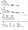 |
Fig. 8 Distributions of offsets (∆v; see Eq. (5)) from best-fit models for each frequency band. |
| In the text | |
|
Fig. 9 Best-fit parameters from the ageing model fits to the stripped tails. Data points are coloured according to galaxy and are consistent between panels. Top: distribution of best-fit injection spectral indices on a galaxy-by-galaxy basis. Error bars correspond to 68% credible regions from the posterior distribution. Bottom: best-fit break frequency as a function of distance along the tail. Each marker corresponds to a single measurement for an individual galaxy, and error bars span the 68% credible region. In the ℓ = 0 bin, upper limits correspond to galaxies with purely power-law spectra and are shown at vb = 10 GHz, which is the upper limit of our prior distribution. To improve readability, in each distance bin data points are randomly shifted along the x-axis according to a Gaussian distribution with µ = 0 and σ = 0.5 kpc. |
| In the text | |
|
Fig. 10 Radiative age versus projected distance along the tail for each of the galaxies in our sample. For each distance bin we plot three estimates of radiative age, corresponding to assumed magnetic field strengths of 1.96 (minimum-loss field), 6, and 10 µG. The radiative age increases monotonically with decreasing magnetic field strength. For each assumed magnetic field strength, we show the best-fit linear relationship between the radiative age and the distance along the tail, which gives an estimate for the projected bulk velocity of cosmic rays along the tail. Data markers and best-fit lines are coloured according to the best-fit projected velocity. |
| In the text | |
|
Fig. A.1 Radio continuum spectra and best-fit ageing model along the stripped tail of NGC4858, fit only to the 144, 400, and 700 MHz data. Panels follow the same formatting as Fig. 7. |
| In the text | |
|
Fig. A.2 Radio continuum spectra for distance bins that show an excess of 1.5 GHz emission relative to the ageing model. Data points correspond to observed flux densities, grey shading corresponds to the ageing model, dashed gold line shows the best-fit power-law component, and the gold shading shows the composite ageing plus power-law model. Each panel lists the best-fit SFR required in order to reproduce the observed flux density excess at 1.5 GHz. |
| In the text | |
|
Fig. A.3 SFR derived from observed Hα + NII emission in the tail, for a grid of different assumed values for the [NII]-to-Hα- ratio and ƒSF. We also plot 1σ, 2σ, and 3σ contours for the ‘required’ SFRs from the composite fits shown in Fig. A.2. |
| In the text | |
|
Fig. B.1 Radio – optical overlay images for the galaxy NGC4848. Background image is a three-colour grz image from the Legacy Surveys (Dey et al. 2019). Contour levels begin at 2.5 × rms and increase by a factor of three with each step. In the lower left we show the common FWHM beam size of 6.5″. In each panel we also overlay the galaxy disc aperture (dashed ellipse) and the apertures used to measure radio continuum flux densities along the tail (solid rectangles). |
| In the text | |
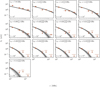 |
Fig. B.2 Tail spectral fitting results for NGC4848. See Fig. 7 for details. |
| In the text | |
|
Fig. B.3 MCMC fitting results for the ageing model along the tail. |
| In the text | |
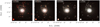 |
Fig. B.4 NGC4853. See Fig. B.1 for details. |
| In the text | |
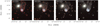 |
Fig. B.5 NGC4858. See Fig. B.1 for details. |
| In the text | |
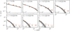 |
Fig. B.6 Tail spectral fitting results for NGC4858. See Fig. 7 for details. |
| In the text | |
|
Fig. B.7 MCMC fitting results for the ageing model along the tail. |
| In the text | |
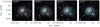 |
Fig. B.8 NGC4911. See Fig. B.1 for details. |
| In the text | |
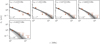 |
Fig. B.9 Tail spectral fitting results for NGC4911. See Fig. 7 for details. |
| In the text | |
|
Fig. B.10 MCMC fitting results for the ageing model along the tail. |
| In the text | |
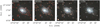 |
Fig. B.11 IC3913. See Fig. B.1 for details. |
| In the text | |
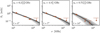 |
Fig. B.12 Tail spectral fitting results for IC3913. See Fig. 7 for details. |
| In the text | |
|
Fig. B.13 MCMC fitting results for the ageing model along the tail. |
| In the text | |
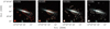 |
Fig. B.14 IC3949. See Fig. B.1 for details. |
| In the text | |
 |
Fig. B.15 IC4040. See Fig. B.1 for details. |
| In the text | |
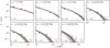 |
Fig. B.16 Tail spectral fitting results for NGC4858. See Fig. 7 for details. |
| In the text | |
|
Fig. B.17 MCMC fitting results for the ageing model along the tail. |
| In the text | |
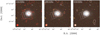 |
Fig. B.18 KUG1250+276. See Fig. B.1 for details. |
| In the text | |
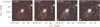 |
Fig. B.19 KUG1255+275. See Fig. B.1 for details. |
| In the text | |
 |
Fig. B.20 Tail spectral fitting results for NGC4858. See Fig. 7 for details. |
| In the text | |
|
Fig. B.21 MCMC fitting results for the ageing model along the tail. |
| In the text | |
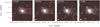 |
Fig. B.22 KUG1255+283. See Fig. B.1 for details. |
| In the text | |
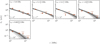 |
Fig. B.23 Tail spectral fitting results for KUG1255+283. See Fig. 7 for details. |
| In the text | |
|
Fig. B.24 MCMC fitting results for the ageing model along the tail. |
| In the text | |
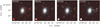 |
Fig. B.25 KUG1256+287B. See Fig. B.1 for details. |
| In the text | |
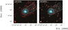 |
Fig. B.26 KUG1257+288B. See Fig. B.1 for details. |
| In the text | |
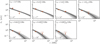 |
Fig. B.27 Tail spectral fitting results for NGC4858. See Fig. 7 for details. |
| In the text | |
|
Fig. B.28 MCMC fitting results for the ageing model along the tail. |
| In the text | |
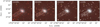 |
Fig. B.29 KUG1258+279A. See Fig. B.1 for details. |
| In the text | |
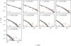 |
Fig. B.30 Tail spectral fitting results for KUG1258+279A. See Fig. 7 for details. |
| In the text | |
|
Fig. B.31 MCMC fitting results for the ageing model along the tail. |
| In the text | |
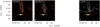 |
Fig. B.32 KUG1258+287. See Fig. B.1 for details. |
| In the text | |
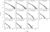 |
Fig. B.33 Tail spectral fitting results for KUG1258+287. See Fig. 7 for details. |
| In the text | |
|
Fig. B.34 MCMC fitting results for the ageing model along the tail. |
| In the text | |
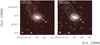 |
Fig. B.35 KUG1259+279. See Fig. B.1 for details. |
| In the text | |
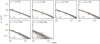 |
Fig. B.36 Tail spectral fitting results for KUG1259+279. See Fig. 7 for details. |
| In the text | |
|
Fig. B.37 MCMC fitting results for the ageing model along the tail. |
| In the text | |
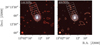 |
Fig. B.38 KUG1259+284. See Fig. B.1 for details. |
| In the text | |
 |
Fig. B.39 Tail spectral fitting results for KUG1259+284. See Fig. 7 for details. |
| In the text | |
|
Fig. B.40 MCMC fitting results for the ageing model along the tail. |
| In the text | |
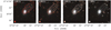 |
Fig. B.41 MRK0053. See Fig. B.1 for details. |
| In the text | |
 |
Fig. B.42 Tail spectral fitting results for MRK0053. See Fig. 7 for details. |
| In the text | |
|
Fig. B.43 MCMC fitting results for the ageing model along the tail. |
| In the text | |
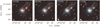 |
Fig. B.44 MRK0056. See Fig. B.1 for details. |
| In the text | |
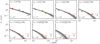 |
Fig. B.45 Tail spectral fitting results for MRK0056. See Fig. 7 for details. |
| In the text | |
|
Fig. B.46 MCMC fitting results for the ageing model along the tail. |
| In the text | |
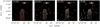 |
Fig. B.47 MRK0057. See Fig. B.1 for details. |
| In the text | |
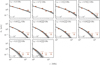 |
Fig. B.48 Tail spectral fitting results for MRK0057. See Fig. 7 for details. |
| In the text | |
|
Fig. B.49 MCMC fitting results for the ageing model along the tail. |
| In the text | |
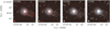 |
Fig. B.50 MRK0058. See Fig. B.1 for details. |
| In the text | |
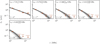 |
Fig. B.51 Tail spectral fitting results for MRK0058. See Fig. 7 for details. |
| In the text | |
|
Fig. B.52 MCMC fitting results for the ageing model along the tail. |
| In the text | |
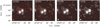 |
Fig. B.53 D100. See Fig. B.1 for details. |
| In the text | |
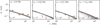 |
Fig. B.54 Tail spectral fitting results for D100. See Fig. 7 for details. |
| In the text | |
|
Fig. B.55 MCMC fitting results for the ageing model along the tail. |
| In the text | |
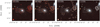 |
Fig. B.56 GMP2601. See Fig. B.1 for details. |
| In the text | |
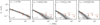 |
Fig. B.57 Tail spectral fitting results for GMP2601. See Fig. 7 for details. |
| In the text | |
|
Fig. B.58 MCMC fitting results for the ageing model along the tail. |
| In the text | |
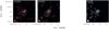 |
Fig. B.59 GMP3618. See Fig. B.1 for details. |
| In the text | |
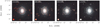 |
Fig. B.60 GMP5226. See Fig. B.1 for details. |
| In the text | |
Current usage metrics show cumulative count of Article Views (full-text article views including HTML views, PDF and ePub downloads, according to the available data) and Abstracts Views on Vision4Press platform.
Data correspond to usage on the plateform after 2015. The current usage metrics is available 48-96 hours after online publication and is updated daily on week days.
Initial download of the metrics may take a while.