| Issue |
A&A
Volume 681, January 2024
|
|
|---|---|---|
| Article Number | A46 | |
| Number of page(s) | 17 | |
| Section | Extragalactic astronomy | |
| DOI | https://doi.org/10.1051/0004-6361/202347413 | |
| Published online | 08 January 2024 | |
Total mass slopes and enclosed mass constrained by globular cluster system dynamics
1
Department of Astrophysics, University of Vienna, Türkenschanzstraße 17, 1180 Vienna, Austria
e-mail: tadeja.versic@univie.ac.at
2
European Southern Observatory, Karl-Schwarzschild Strasse 2, 85748 Garching, Germany
3
AURA for the European Space Agency, ESA Office, Space Telescope Science Institute, 3700 San Martin Drive, Baltimore, MD 21218, USA
Received:
10
July
2023
Accepted:
14
September
2023
We study the total-mass density profiles of early-type galaxies (ETGs: ellipticals and lenticulars) with globular clusters (GCs) as kinematic tracers. The goal of this work is to probe the total mass distribution, parameterised with a double power-law profile, by constraining the parameters of the profile with a flexible modelling approach. To that end, we leverage the extended spatial distribution of GCs from the SLUGGS survey (⟨RGC, max⟩∼8 Re) in combination with discrete dynamical modelling. We use discrete Jeans anisotropic modelling in cylindrical coordinates to determine the velocity moments at the location of the GCs in our sample. Assuming a Gaussian line-of-sight velocity distribution (LOSVD) and a combination of informative and uninformative priors we use a Bayesian framework to determine the best-fit parameters of the total mass density profile and orbital properties of the GCs. We find that the choice of informative priors does not impact the enclosed mass and inner slope measurements. Additionally, the orbital properties (anisotropy and rotation of the dispersion-dominated GC systems) minimally impact the measurements of the inner slope and enclosed mass. A strong presence of dynamically-distinct subpopulations or low numbers of kinematic tracers can bias the results. Owing to the large spatial extent of the tracers our method is sensitive to the intrinsic inner slope of the total mass profile and we find ᾱ = −1.88 ± 0.01 for 12 galaxies with robust measurements. To compare our results with literature values we fit a single power-law profile to the resulting total mass density. In the radial range 0.1–4 Re our measured slope has a value of ⟨γtot⟩= − 2.22 ± 0.14 and is in good agreement with the literature. Due to the increased flexibility in our modelling approach, our measurements exhibit larger uncertainties, thereby limiting our ability to constrain the intrinsic scatter σγ.
Key words: galaxies: halos / galaxies: elliptical and lenticular / cD / galaxies: kinematics and dynamics / galaxies: structure
© The Authors 2023
 Open Access article, published by EDP Sciences, under the terms of the Creative Commons Attribution License (https://creativecommons.org/licenses/by/4.0), which permits unrestricted use, distribution, and reproduction in any medium, provided the original work is properly cited.
This article is published in open access under the Subscribe to Open model. Subscribe to A&A to support open access publication.
1. Introduction
In the current cosmological framework, galaxy formation is driven by the coalescence of gas in the dark matter overdensities of large-scale structures (White & Rees 1978). In the context of ΛCDM cosmology, the total mass of galaxies is dominated by dark matter on large scales, while the inner regions r ≲ 1 − 2 Re1 are dominated by stars (Cappellari et al. 2013). Therefore, in order to understand the mass content of these galaxies we need extended kinematic tracers of the gravitational potential.
Early analytic efforts to characterise the mass distribution within early-type galaxies (ETGs: ellipticals and lenticulars) were based on the dynamical formalism of the Jeans equations (Jeans 1922) and implementing the effects of violent relaxation (Lynden-Bell 1967). With additional assumptions of spherical symmetry and isotropic orbital distribution, the resulting radial density profile for both dark matter and baryons was found to have a power-law distribution ρ(r)∝rγtot with a slope of −2. A similar, isothermal, distribution was also found for gas-rich late-type galaxies (LTGs; see review in Courteau et al. 2014) and it results in the flattening of the circular rotation curves first reported by Rubin et al. (1970).
The first studies with gravitational lensing of ETGs found that the total mass distribution within the Einstein radius (∼Re/2) can be closely approximated by a single power law with a narrow scatter and a profile that is slightly steeper than an isothermal sphere with a slope of −2 (Auger et al. 2010; Barnabè et al. 2011; Sonnenfeld et al. 2013). This trend was initially determined for the strongest gravitational lenses, i.e., the most massive galaxies. Subsequently, a similar trend was confirmed for lower-mass galaxies using dynamical modelling (e.g., Alabi et al. 2016; Poci et al. 2017; Bellstedt et al. 2018, hereafter A16, P17, B18). In the case of ETGs, the apparent tendency that two non-isothermal distributions of stars and dark matter ‘conspire’ in a close-to-isothermal slope has been a point of great discussion. The ‘bulge-halo conspiracy’ was found to hold only on certain mass scales, suggesting that galaxy feedback processes might play a role (Dutton & Treu 2014, and references therein).
The flat velocity dispersion profile found within 1 Re of ETGs has been linked to the dry major mergers as the main formation channels of these gas-poor systems. Through simulated binary mergers, Remus et al. (2013) showed that the inner slope γtot ∼ −2 acts as a natural attractor, and once in place, only a major merger with a high gas fraction can modify the total mass density slope. They found that the larger the fraction of in-situ formed stars the steeper the total density profile. They link this with the dissipationless nature of gas, which sinks in the centre of the merged galaxy to form a new population of more centrally concentrated stars, thereby steepening the total mass slope.
Poci et al. (2017) investigated the correlations between the inner slope and stellar kinematic properties and found for galaxies with log σe ≳ 2.1, the stellar velocity dispersion at 1 Re, that the inner slope is constant. Recently, Zhu et al. (2024) extended the study to late-type galaxies (LTGs) and found morphological and mass dependence of the γtot in the sample of MANGA galaxies. LTGs with log σe < 2.2 show an increasingly shallower total mass density profile in contrast with ETGs. They also found a steeper slope with increasing age of the stellar component at a fixed value of σe.
In LTGs, the cold gas traces the total mass distribution out to few Re, while most ETGs have already depleted their main gas reservoir, and observations of the centrally concentrated inner stellar component are needed to constrain the potential. The stellar surface brightness profile drops rapidly and it becomes observationally challenging to observe beyond a few Re. However, all galaxies have their inner and extended outer halos populated by globular clusters (GCs; Harris 1991, and references therein). Owing to their compact size and high stellar surface brightness they can be observed in nearby galaxy clusters (e.g., Côté et al. 2004; Jordán et al. 2007a) and they probe the gravitational potential in the outer regions of galaxies and clusters (e.g., Chaturvedi et al. 2022). Several literature studies have utilised these tracers to carry out dynamical modelling and used the distinct origin and dynamical properties of the GCs populations to constrain the enclosed mass and to break the mass-anisotropy degeneracy (e.g., Napolitano et al. 2014; Zhu et al. 2016).
In this paper we carry out discrete anisotropic Jeans modelling accounting for the observed flattening of the GC systems (GCS) to investigate the inner slope of the total mass profile and the virial mass. In Sect. 2 we introduce the sample of GCs used throughout the paper and discuss the source of photometry and kinematics. Then we discuss the modelling of the tracer density profile in Sect. 3, one of the key components of the dynamical modelling. We introduce the dynamical modelling approach we adopted, focusing on the Bayesian inference and different modelling set-ups in Sect. 4, followed by a discussion of the results and exploration of potential biases in our modelling approach in Sect. 5. In Sect. 6 we compare the results with literature values, and discuss our results in Sect. 7. Section 8 presents and summarises our main conclusions.
2. Sample of globular cluster systems
In this section we introduce the data used throughout this work. For dynamical modelling, we need kinematic data as well as information on the spatial distribution of the tracer population. We used the sample of the GC radial velocities (RV) from the SAGES Legacy Unifying Globulars and GalaxieS (SLUGGS; Brodie et al. 2014) survey that observed 27 nearby galaxies. First, we discuss the properties of the RV sample and define the kinematic flags based on the visual inspections of the GC velocities. Second, we present the sources of GC photometry for 21 galaxies used to determine the tracer density profile in Sect. 3. The observed properties of the 21 galaxies we modelled in this work are presented in Table 1.
Basic information for the 21 galaxies from the SLUGGS survey modelled in this work.
2.1. Kinematic datasets
The kinematic tracers from the SLUGGS dataset have a typical spatial extent of ∼8 Re up to Rmax ∼ 15 Re and a median of 80 GCs per galaxy, varying from 20 to 600 GCs per individual galaxy. The median error of the radial velocities is 10–15 km s−1, representing around 10% of the typical velocity dispersion of a GCS for SLUGGS galaxies. The SLUGGS catalogue excludes foreground stars and background galaxies based on the phase-space diagram (Forbes et al. 2017). Additionally, ultra-compact dwarfs (UCDs) are flagged, and we excluded them from the following analysis. UCDs can be misidentified as the bright tail of the GCs due to their compact size and magnitude, but they have a different origin, and therefore different spatial distribution and orbital properties (e.g., UCDs in NGC 5128: Dumont et al. 2022).
2.1.1. NGC 5846
A special remark is needed for galaxy NGC 5846, which is the brightest cluster galaxy and has three bright companions (NGC 5846A, NGC 5845, and NGC 5850). The projected phase space distribution of GCs belonging to NGC 5846 from the SLUGGS survey and the locations of all four galaxies are shown in Fig. 1.
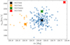 |
Fig. 1. Position of the GCs from the SLUGGS survey are shown as blue and orange points. The orange points are selected based on their position as more likely belonging to NGC 5845, and the blue points show the NGC 5846 GCs used in this work. The positions and systemic velocities shown as coloured crosses for the four galaxies are from Simbad (https://simbad.unistra.fr/simbad/). |
The spatial and velocity distribution of NGC 5846A and NGC 5845 overlap with those of NGC 5846. In Fig. 1 there is a clear elongation of the GCS in the direction of NGC 5845, but the contamination from NGC 5846A is not as apparent in this phase-space diagram. To estimate the contamination of the GC catalogue for NGC 5846 we first estimated the number of GCs for each of these galaxies based on their absolute V-band magnitude. We used the observed correlations between the number of GCs and the absolute V-band magnitude of its host galaxy in a high-density cluster environment (e.g., Zepf et al. 1994; Kissler-Patig 1997). We estimate that NGC 5846A hosts fewer than 100 GCs; for NGC 5845 we estimate ∼300 GCs, and NGC 5846 is expected to host ∼2500 GCs. The GCs from NGC 5845 thus have a much stronger contribution to the contamination than the GCs from NGC 5846A. To remove potential GCs belonging to NGC 5845 we removed clusters at α < 226.52° from the kinematic dataset of NGC 5846. A more sophisticated selection and additional removal of NGC 5846A GCs is beyond the scope of this work.
2.2. Kinematic flags
Strong rotation, substructures (non-relaxed populations), and a small number of kinematic tracers or GC subpopulations with distinct kinematics can bias the results of the dynamical modelling. Before proceeding with the modelling we visually inspected the velocity distribution of the GCS for all galaxies.
We focused on the radial variation of mean velocity and velocity dispersion and on the 2D velocity field of the GCs, similar to the one shown in the left panel of Fig. 2 for NGC 3377. We visually inspected the regularity of the velocity field looking for the presence of strong rotation signatures, cold comoving groups, observationally biased sparse sampling or other peculiar features.
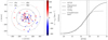 |
Fig. 2. Example of spatial and magnitude distribution of the kinematic tracers. Both were used to determine an observationally unbiased sample of GCs to construct the tracer density profile for each galaxy. The left panel shows the spatial distribution of the GCs in NGC 3377 centred at the coordinates of the host galaxy and aligned with the photometric position angle. The GCs are colour-coded by their velocity corrected for the systemic velocity of the galaxy. The kinematic tracers extend beyond 9 Re. The solid grey line in the right panel shows the GCLF of NGC 3377. The dashed black curve shows the arbitrarily scaled theoretical GCLF; the turn-over magnitude is indicated with a vertical solid black line. The vertical dotted line shows the magnitude completeness of the sample, determined as described in the text. |
Focusing on these features we defined four flags: Good (9/21) and Good w. rot. (4/21) for GCSs showing a highly regular velocity field, and that are either dispersion-dominated or show non-negligible rotation, respectively; Subpop. (subpopulations, 3/21) for galaxies showing distinct kinematic subpopulations (such as the blue and red GC populations in NGC 1407, Romanowsky et al. 2009) or cold comoving groups that can inflate their velocity dispersion; and Pecul. (peculiar, 5/21) for galaxies that have on average the lowest number of GCs among the SLUGGSs galaxies and show an irregular velocity field. The galaxy flags are shown in Col. 10 of Table 1.
2.3. Photometric datasets
One of the inputs for the dynamical modelling is the spatial distribution of the kinematic tracers (i.e., tracer density profile), and photometry is crucial to accurately characterise it. The SLUGGS catalogue provides photometry in the Sloan g and z bands for the 12 galaxies that can be used to construct accurate tracer density profiles. For the remaining galaxies we utilised either literature photometry, when available, or the parameters of the fitted number density profile. With the literature photometric information, we could construct the tracer density profiles for nine additional galaxies. The source of photometry or tracer density profile for each of the galaxies is presented in the last column of Table 1.
Eight galaxies in the SLUGGS survey belong to the Virgo galaxy cluster. This nearby galaxy cluster (d ≃ 16.5 Mpc) was extensively studied with the HST Advanced Camera for Surveys (ACS) as part of the ACS Virgo Cluster Survey (ACSVCS; Côté et al. 2004). We used the photometry in the F475W (≃Sloan g) and F850LP (≃Sloan z) bands of six galaxies in the survey. ACSVCS targeted only the innermost regions of the galaxies and the spatial extent of their tracers is limited to Rmax ∼ 100″, which translates to ∼3 Re for a typical galaxy in our sample. For three of the galaxies that we model, only the best-fitting parameters of the tracer density profile were available.
3. Modelling tracer density profile
The key component of any dynamical modelling is an accurate spatial distribution of the tracer population. For the dynamical modelling approach used in this work, the input tracer density profile is needed in the form of multi-Gaussian expansion (MGE, Emsellem et al. 1994) and in this section, we explain how we constructed MGEs for the SLUGGS galaxies.
We applied the analysis to the 18 SLUGGS galaxies, for which the photometry of the GCs is available in the literature (see Table 1). The sources of photometry used in this work are heterogeneous and assessing the magnitude completeness and observational footprint from the photometric images was not possible. That is why we used the observed GC luminosity function (GCLF) to asses the magnitude completeness and radial variation of PAGCS (position angle) for spatial completeness. The two steps are applied only to the photometric dataset as dynamical modelling is less sensitive to incompleteness in the kinematic sample.
Early-type galaxies show the presence of multiple populations of GCs (Jordán et al. 2007b, and references therein) found in their colour distribution. Fahrion et al. (2020) studied the kinematic properties of GCs in a sample of ETGs from the Fornax 3D survey (Sarzi et al. 2018) in a mass range similar to that of the SLUGGS ETGs. Splitting them into red and blue populations, based on their colour, they found that the velocity dispersions of both populations agreed within their measurement uncertainties. Building on those findings and the work done by A16, Posti & Fall (2021), and Bílek et al. (2019), we treated the red and blue GCs as one population in our dynamical modelling. Notable exceptions where this treatment breaks down are the central dominant galaxies NGC 1407, NGC 4486, and NGC 5846. These galaxies have been shown to have very different accretion histories to other galaxies (e.g., De Lucia & Blaizot 2007; Oliva-Altamirano et al. 2015) and much richer population of GCs (Harris et al. 2017). As Chaturvedi et al. (2022) showed in a study of the central galaxy of the Fornax cluster, these galaxies host a population of blue (metal-poor) GCs that trace better the group or cluster potential. We discuss these three galaxies further in Sect. 7.2.1.
For the three galaxies with literature studies on the GCs number density profile, we used the parameters of the fit. In Sect. 3.4 we focus on a close pair of Leo II galaxies, for which the GC density profile was investigated with two different methods in Kartha et al. (2016).
3.1. Magnitude completeness
We used the observed GCLF to determine the limiting magnitude. Sources fainter than the limiting magnitude are strongly affected by incompleteness. Including them in the analysis of the tracer density profile would introduce a bias by mimicking a shallower profile close to the centre of the galaxy as the galaxy light becomes brighter than the faint GCs.
The GCLF for ETGs is closely approximated by a Gaussian distribution (Rejkuba 2012, and references therein). The mean absolute magnitude of the GCLF, the turn-over magnitude (TOM), is constant for massive ETGs within ±0.2 mag (e.g., Harris et al. 2014; Villegas et al. 2010) and has even been used to determine precise distances to galaxies (e.g., Jordán et al. 2005). The width of the GCLF, σGCLF, depends on the total mass of the galaxy with a significant scatter at the faint end (Villegas et al. 2010).
To determine a magnitude-complete sample of GCs, we compared the observed cumulative GCLF with the theoretical Gaussian function, assuming TOMV = −7.5 mag or TOMz = −8.5 mag and a spread of σGCLF ∼ 1.2 mag computed from the absolute magnitude of the galaxy in the B band and relation found in Jordán et al. (2007b). The theoretical luminosity function is normalised to match the number of clusters up to the limiting magnitude in an iterative approach. For each galaxy we computed the square of the residuals between the observed cumulative GCLF and theoretical function and we set the magnitude limit where the residuals exceed 1σ. This is shown in the right panel of Fig. 2 for NGC 3377. The observed GCLF of this galaxy becomes strongly affected by the incompleteness at the limiting magnitude of 23.8, shown with the grey dotted line in the right panel of Fig. 2. The limiting magnitudes and radial truncation for all of the galaxies are presented in Table 2 together with the results of the Sérsic fit.
Results from the analysis of the tracer density profile fitting and completeness.
3.2. Spatial completeness
After determining the magnitude limit we analysed the radial variation of PAGCS (increasing from north to east) and flattening defined as qGCS = 1 − e = 1 − b/a to understand the spatial completeness and measure both parameters. In the axisymmetric dynamical modelling used in this work, the axis of symmetry has to be aligned with the position angle and can be flattened along the vertical axis.
The analysis was performed in the projected Cartesian coordinate system (x, y), where x is in the direction of west and y is north. For the transformation from the equatorial coordinates of the GCs (αi, δi) we used the following equations from van de Ven et al. (2006):


Here α0, δ0 are the coordinates of the centre of the galaxy. The scale factor r0 = 180/π × 3600 converts x and y from radians to arcsec.
The values of PAGCS and qGCS are computed by constructing an inertial tensor from the GC positions (x, y). The eigenvectors of the tensor are aligned along the semi-major axes. We assume that the intrinsic position angle of each GCS is constant with radius and that any deviations we measure are introduced by the observational footprint in the SLUGGS survey. We take the radius where the PAGCS and qGCS change rapidly as the maximal completeness radius and we present it in Col. (3) of Table 2 in units of Re. Columns (4) and (5) show the recovered PAGCS and qGCS of the spatially and magnitude complete sample.
3.3. Sérsic fits
After establishing a spatially and magnitude complete sample we ere able to bin the photometric data for each galaxy and fit the MGEs to the binned profile. However, binned profiles are stochastic and the number of bins is often small. So instead we chose to fit an analytic Sérsic function to the binned data as an intermediate step. To account for the flattening of the GCS we did not bin in spherical radii; instead, we used the elliptical radius for each GC  .
.
We investigated two binning strategies: logarithmically spaced bins and bins with an equal number of GCs. For each binning strategy we additionally created five different binned profiles, varying the number of bins or number of GCs per bin. This step was motivated by the large variation in the number of GCs per galaxy. It also enabled us to compare the resulting best-fit parameters of the analytic function in order to ensure the binning introduces minimal bias. Then we fitted the analytic Sérsic function to the binned number density Σ [NGC arcsec−2]
where ν0 is the normalisation in the units of NGC arcsec−2, Re is the effective radius, and n is the Sérsic index. For the value of bn we used the asymptotic expansion for bn = 2n − 1/3 + 4/(405n)+46/(25515n2) from Ciotti & Bertin (1999). This approach yields good results even in the presence of low-number statistics with a small number of bins.
To fit the Sérsic function we used a Bayesian framework, with flat priors on the free parameters: nGCS and Re, GCS, and a Gaussian likelihood. The best-fit parameters and the posteriors were sampled using EMCEE (Foreman-Mackey et al. 2013) a Python implementation of the Goodman & Weare (2010) affine-invariant Markov chain Monte Carlo (MCMC) ensemble sampler.
As an example, the best-fit Sérsic model for NGC 3377 is shown in Fig. 3. The black points with respective uncertainties represent the binned data. The solid red line is the best-fit model and grey-shaded regions are 1σ and 3σ uncertainty regions. The full results of the fits are presented in Table 2 in Cols. (6) and (7).
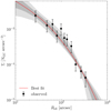 |
Fig. 3. Sérsic fit to the binned tracer density profile for NGC 3377 in elliptical radius. The binned profile is represented by black points. The best-fit model is shown with the solid red line with 1 and 3σ uncertainty regions indicated with dark and light grey shaded regions, respectively. |
3.4. MGE decomposition
The last step is to represent the tracer density profile in the MGE format required for the dynamical models we use later. For the 18 galaxies to which we fitted Sérsic profiles directly, we drew samples of the Sérsic parameters from their posteriors and used them to evaluate the profile at each radius. This step mimics observational noise and provides a more realistic treatment of the tracer density profile. We used mgefit, an implementation of the MGE algorithm by Cappellari (2002).
Three galaxies, NGC 720, NGC 3607, and NGC 3608, only have parameters of the Sérsic profile reported in the literature and do not have GCs photometry available. For these galaxies we did not have posteriors to draw from, so our approach was necessarily different. We generated random samples of n and Re assuming a Gaussian distribution centred at the best-fit values presented in the literature, generated the perturbed Sérsic profile, and proceeded in the same way as before. For these galaxies, we took PAGCS from the main stellar component and qGCS from the literature studies. The information is listed in Table 2.
3.4.1. NGC 3607 and NGC 3608
NGC 3607 and NGC 3608 are part of the Leo II group. They are a close pair with a projected distance of 39 kpc and a relative difference in the systemic velocity of ∼260 km s−1 (Brodie et al. 2014). The velocity dispersion of the GCS, of the order of 150 km s−1 (Kartha et al. 2016), means that membership cannot be assigned based on velocities alone. To this end, we used the results from Kartha et al. (2016), where the properties of GCS were investigated in a systematic way, and two different methods were used to determine the distribution of GCS in the two galaxies (see their Sect. 4).
The authors find that PAGCS and eGCS for NGC 3607 are consistent between the different methods. The recovered PAGCS for NGC 3608 differs by more than 2σ between the two methods. We adopted the results from their major-axis method (see their Sect. 4.2) for both galaxies, and we used the Sérsic parameters computed with this method (Table 2). We found this method better matched our analysis of the PAGCS of NGC 3608 based on the kinematic sample.
4. Discrete dynamical modelling
In this section we introduce the dynamical modelling approach used in this work. First, we present the anisotropic Jeans models followed by the Bayesian inference to find best-fit parameters. The results and robustness tests against the modelling assumptions are presented in the next section.
4.1. Axisymmetric Jeans anisotropic MGE models
Most ETGs in the nearby universe are closely approximated as axisymmetric systems in a steady state. Jeans equations derived from the collisionless Boltzmann equation in cylindrical coordinates (R, z, ϕ) have been used extensively in the literature to determine the dynamical properties and mass profiles of galaxies using a variety of different tracers (PNe, GCs, stellar and gas kinematics). The recent study of simulated GCS by Hughes et al. (2021) investigated the accuracy of Jeans models applied to these discrete potential tracers of LTGs and showed its robustness in recovering the enclosed mass.
The axisymmetric Jeans anisotropic MGE (JAM) formalism was introduced by Cappellari (2008). Within the formalism, the velocity ellipsoid is cylindrically aligned and the velocity anisotropy has the form  . To compute the first velocity moments an additional assumption on the rotation of the dynamical tracers is incorporated through the κ parameter. It encapsulates the relative contributions of ordered and random motions:
  . Through the inclination angle, the intrinsic velocity moments are projected along the line of sight. In this work we assume that the GCS is aligned spatially with the inner stellar component, and use the inclination of the latter as presented in the literature from various sources and summarised in Table 1.
The tracer and mass densities are represented using the MGE method. In this method we represent the number and mass densities as a series of Gaussians. The benefits of this parametrisation are that it is flexible and computationally fast and stable.
The models provide the first and second velocity moments  at a given position on the plane of the sky. The velocity dispersion is given by
  . This enables discrete dynamical modelling, through the assumption of local line-of-sight velocity distribution (LOSVD). There are three main advantages of the discrete approach over binning velocities in radial bins: the number of kinematic data points constraining the model is higher, biases due to an arbitrary binning strategy are removed, and contaminants that could bias binned velocity moments can be self-consistently modelled (e.g., Watkins et al. 2013; Hénault-Brunet et al. 2019). This simplified assumption is reasonable given the quality and size of the dataset, and it has been used in the literature to model discrete kinematic datasets (e.g., Zhu et al. 2016). Read et al. (2021) compared different modelling techniques on simulated datasets (spherical Jeans equations, distribution function models, and higher virial moments) and found good agreement in the recovered mass profile for the different modelling techniques.
4.2. Gravitational potential
In this work the total mass in a galaxy (luminous and dark matter) is assumed to follow a spherical double power-law profile (as done in Cappellari et al. 2013, 2015; Poci et al. 2017; Bellstedt et al. 2018). We assume the functional form
where ρs represents scale density and rs scale radius. The inner total mass slope, parameterised by α, transitions to an outer slope fixed at −3.
4.3. Bayesian inference
We use Bayesian inference to find the best-fit models. Each GC is treated independently and no binning in velocities is used to obtain the mean velocity and velocity dispersion profile.
4.3.1. Likelihood
Given the assumption of a Gaussian LOSVD the likelihood is
where  is the dispersion of the LOSVD at the position of the ith GC convolved with the measurement uncertainty. At the position of each GC, this constitutes the likelihood of the measured velocity (vi, δvi) given the free model parameters θ.
4.3.2. Priors and summary of the modelling set-ups
In this analysis we use both uninformative (flat) priors and informative (Gaussian) priors. The informative priors were necessary to break the degeneracy in the modelled parameters (in particular between ρs and rs) without the need for fixing one of them. The Gaussian function was chosen for its simplicity and symmetry. To test and ensure that the priors are not driving the resulting posteriors, we run two models with different prior widths.
We consider three different model set-ups: models A, B, and C. They differ in the number of free parameters and the widths of Gaussian priors. In models A and B we vary only the three parameters of the total mass profile in Eq. (6) (ρs, rs, α) and change the prior widths between the two models. In model C we additionally vary rotation and velocity anisotropy, and thus have five free parameters:(ρs, rs, α, βz, κ). The modelling set-ups and choices of priors are summarised in Table 3.
Overview of the priors for different set-ups.
The assumption of no rotation and isotropy in models A and B is motivated by the substantial increase in the computational time of the models when βz ≠ 0 and κ ≠ 0. Before proceeding with models A and B we explored the variation in the likelihood on small grid models by varying βz and κ. We found the peak of the likelihood corresponding to very mild radial anisotropy (βz > 0), and the galaxies that were flagged as having strong rotation signatures in Sect. 2.1 have a prominent non-zero peak. We discuss the impact of these assumptions on the recovered parameters of the total mass density in Sect. 5.2.
The parameters ρs and rs can vary by several orders of magnitude; to sample the posterior more efficiently they are sampled in logarithmic space. Other parameters are dimensionless, and even though anisotropy is a strongly asymmetric variable2 we do not reparametrise it as GCSs show only mildly anisotropic orbital distributions, as discussed in Sect. 5.2. The effect our choice of priors has on the posteriors is discussed in Sect. 5.1.
4.3.3. Posterior
Having defined the likelihood and priors, the Bayes theorem gives the expression for the posterior:
Here 𝒫(θ|𝒟) is the posterior for a given set of free parameters θ, ℒ(𝒟i|θ) is the likelihood for the ith GC and p(θ) is the prior.
4.3.4. MCMC set-up
To explore the parameter space and sample the region of best-fitting parameters, we use the EMCEE package, a Python implementation of an affine-invariant ensemble sampler for Markov chain Monte Carlo (MCMC). For models A and B (isotropic and non-rotating) we use 100 walkers and 6000 steps and for model C (free βz and κ) 100 walkers and 2000 steps, due to the increase in the computational time. In both set-ups, 600 steps are discarded as a burn-in phase. We verified that this set-up is longer than several auto-correlation times, and we visually inspected the convergence of the chains. The initial conditions are the same in all runs: log10ρs = −4 [M⊙ pc−3], log10rs = 1.3 [kpc], α = −1.5, and for model C: β = 0.01, κ = 0.1. These initial conditions were informed by prior dynamical modelling of GCs in FCC 167, an ETG of the Fornax galaxy cluster. Given its properties, the modelled galaxy is a good representative of the ETGs in the SLUGGS sample. We explored the robustness of the posteriors against the variations in the initial conditions and found a negligible effect.
5. Results: Fiducial model and robust sample
Now that we have described the dataset and laid out the models we can describe how we applied the models to the data. We applied models A, B, and C to all 21 galaxies in our sample and found that all MCMC chains converged and all posteriors were unimodal. As an example, we show the corner plot for NGC 3377 for the model B set-up in Fig. 4. The parameters ρs and rs are strongly anti-correlated, and the informative priors we imposed help to constrain both but cannot break the degeneracy. The inner slope α is not degenerate with the scale density and radius, but has a tail towards shallower profiles. At such shallow profiles, rs ∼ 1 kpc (within the innermost kinematic tracer), and therefore in these cases the density is effectively a single power-law profile with the slope of −3 (see Eq. (6)).
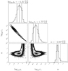 |
Fig. 4. Posterior of model B for NGC 3377. The median and the 1σ percentiles are shown as dashed lines on each of the marginalised posteriors and the corresponding values are given at the top. |
We adopted model B as the fiducial model, following the arguments laid out in this section; the robust sample of galaxies are those with the flags Good and Good w. rot., as introduced in Sect. 2.2. We present the best-fit values of the total mass density profile for the fiducial model in Table 4 for the 19 galaxies we modelled. NGC 1400 and NGC 3607 were not modelled because the literature value of the inclination was not consistent with the projected flattening of their GCSs.
Summary of posterior results from the fiducial set-up, model B.
5.1. Effect of informative priors
To test the robustness of the results against our choice of priors we discuss the marginalised posteriors of models A and B, the two isotropic and non-rotating set-ups, in this section. We focus only on the parameters with informative priors log10ρs and log10rs as the prior for α is the same in both set-ups (see Table 3). The posteriors for the two set-ups are shown in Fig. 5. The top row shows the results for model A and the bottom row for model B (fiducial model), as described in Sect. 4.3. Each column corresponds to a different free parameter of the total density profile: log10ρs on the left and log10rs on the right. The solid grey lines show the marginalised posteriors for each of the modelled galaxies and priors are shown with coloured lines: the blue line shows prior for model A and the orange for model B.
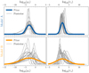 |
Fig. 5. Comparison between informative priors for log10ρs and log10rs as coloured lines for model A and model B and the posteriors for each of the 21 modelled galaxies as grey lines. In fiducial model B the widths of the posteriors are narrower than those of the priors, which indicates that the data is driving the posterior, not the prior. |
The posteriors and priors show similar widths in the top panels for model A making it unclear whether the data or prior are driving the posterior distribution in this case. This motivated us to test the robustness of the informative priors to ensure our choice of prior was not driving the posterior. To this end, we increased the widths of the Gaussian priors on the log10ρs and log10rs parameters, and in the bottom row for model B the prior is wider than the posteriors. This indicates that the data is driving the posterior for this choice of prior. Thus, we adopted model B as the fiducial set-up. This effect is most strongly seen for the log10ρs parameter, while the posteriors in log10rs are narrower than the prior in both instances. For clarity, the inner slope α is not shown in Fig. 5. We compared the values of the slope between the two set-ups and found minimal differences in their posteriors. We performed the same investigation for model C, which includes rotation and anisotropy and found similar behaviour of the posteriors as for model A.
We further explored the impact of informative priors by comparing the resulting enclosed mass for models A and B. To compute the enclosed mass we numerically integrated Eq. (6). We randomly drew 1000 samples from the posterior, computed the enclosed mass profile, and determined the uncertainties at fixed radii: 1 Re, 5 Re and at the radius of the maximum extent of the tracers for literature comparison. In the integration we excluded profiles with α steeper than −3. These result in infinite enclosed mass, and with ≲0.5% of the chains having such extreme values we considered that this selection did not impact our results and conclusions.
The enclosed mass measurements for model B are presented in Table 5 and the comparison between the fiducial and narrow set-up is presented in Fig. 6 within 5 Re. The different symbols correspond to the kinematic flags defined in Sect. 2.2. The black points show galaxies flagged as Good or with strong rotation signatures, the red open symbols denote the galaxies with strong subpopulations, and the blue open symbols are peculiar galaxies with apparent peculiar velocity fields. The dashed line shows the 1–1 relation to guide the eye and is not a fit to the points. This figure demonstrates the negligible effect the prior widths in models A and B have on the enclosed mass. The same is found for enclosed mass at all radii we investigated, with the uncertainties increasing with increasing radius, and it also holds for model C.
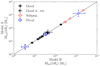 |
Fig. 6. Effect of informative priors on enclosed mass within 5 Re. The black dots and triangles show galaxies flagged as Good and Good w. rot., respectively, as defined in Sect. 2.2. The measurements for these galaxies are robust. The open red diamonds and blue squares are galaxies flagged as Subpop. and Pecul., respectively, and for which the measurements are not robust. The dashed line is a 1–1 line for reference. |
Results from the fiducial run (model B set-up).
5.2. Effects of rotation and velocity anisotropy
After investigating the effects of informative priors on the posterior and enclosed mass here we discuss the impact of anisotropy and rotation of the GCS on the parameters of the total mass distribution. We find the enclosed mass and inner slopes α are consistent between models A, B, and C, suggesting that velocity anisotropy and rotation have a negligible impact on the recovered properties of the total mass profile. A16 studied the GCs of the SLUGGS galaxies and, using a tracer mass estimator (TME, e.g., Watkins et al. 2010)3, they found a minimal contribution (∼6%) to the pressure-supported mass estimate due to rotation (see their Fig. 7) and ∼5% when a different velocity anisotropy for GCs is assumed (see the right panel of their Fig. 5).
This can be seen in Fig. 7 for NGC 3115; we chose to show this galaxy as it shows signs of strong rotation in the kinematics of its GCs. In the figure we compare the velocity moments computed from the best-fit parameters of models B (in black) and C (in red). The blue squares and triangles show the binned velocity dispersion and rotation of the GCs; they are shown for visualisation purposes and were not used in the dynamical modelling. To obtain the binned profiles we assumed a point-symmetric velocity field, characteristic of a relaxed axisymmetric system, and symmetrised the velocities to reduce the noise in each radial bin. We imposed a constant number of GCs in each bin along the semi-major axis and computed the robust mean velocity and velocity dispersion (i.e.,  ) for the kth bin. The drop in the velocity dispersion close to the centre of the galaxy is not realistic, but is due to incompleteness in the radial velocity measurements in the galaxy’s inner region.
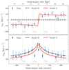 |
Fig. 7. Comparison between the best-fit results from models B and C and the data for NGC 3115 along the semi-major axis of the galaxy. The top panel shows the mean velocity and the bottom the velocity dispersion. The blue triangles and squares show the mean velocity and velocity dispersion of the GCs, respectively. The black dashed line shows the velocity dispersion computed with the best-fit parameters of model B. The solid red line shows the same for model C. The vertical grey lines show multiples of the stellar effective radius for comparison. |
In this galaxy, the rotation of the GCs in the outer parts is  km s−1 and the velocity dispersion is σlos ∼ 130 km s−1. The results for model B are shown as a black dashed line and the velocity moments from CJAM for model C are shown as a solid red curve. In the top panel we see that model C can reproduce the observed rotation well, which by construction is not the case for model B. The velocity dispersion profile is very closely matched by model B in the bottom panel, and model C agrees within the 1σ uncertainties of the data. We can see that in the observing plane, models B and C both agree with the velocity dispersion profile, as seen in the bottom panel.
5.2.1. Velocity anisotropy and rotation measurements
In Fig. 8 we show the anisotropy parameter (top panel) and rotation parameter (bottom panel).
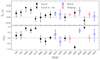 |
Fig. 8. Best-fit velocity anisotropy and rotation from model C. The symbols match those in Fig. 6; the black points are the galaxies with robust measurements and the open symbols those without. The top panel shows the velocity anisotropy for each galaxy and the bottom panel shows the rotation parameter κ. The error bars highlight the 16th and 84th percentile uncertainty on the measurement. The dashed grey line shows the isotropic βz = 0 and non-rotating κ = 0 values for reference. |
We find that most galaxies have a velocity anisotropy consistent with zero, consistent with the assumptions in models A and B. NGC 1023 and 2768 deviate at the level of 3σ, showing more radial orbits (βz > 0). We also find that most GCs are consistent with having negligible rotation, with the exception of those we flagged as having strong rotation signatures (black triangles). Two galaxies were not flagged as showing a strong rotation signature in the velocity field of their individual GCs (NGC 2768 and NGC 4494), but the model prefers strong κ ≠ 0.
5.3. Definition of the robust sample
In this work we present robust results for 12 galaxies out of the initial 21; they are flagged as Good (8 galaxies) and Good w. rot. (4 galaxies) in Table 5. In the rest of the paper we refer to them as ‘robust measurements’.
In our analysis we identified galaxies with strong rotation signatures, a small number of GCs, or a strong presence of subpopulation in their GCS. Three galaxies, NGC 1407, NGC 4486 (M 87), and NGC 5846, are central galaxies in their respective groups, and literature studies have identified a strong presence of dynamically distinct populations. We flagged them as Subpop. (subpopulations) based on the differences in the kinematic properties between the red and blue GCs. We flag four galaxies, NGC 4374, NGC 4459, NGC 4526, and NGC 7457, as Pecul., owing to the peculiar signatures in the kinematics of their GCs. We discuss the individual galaxies with these flags in more detail in Sect. 7.2. In the analysis that follows we show the results for these two classes with open symbols for completeness.
5.4. Single power-law slope of the total mass density
Here we introduce the method used to determine the single power-law slope from Eq. (6); we present the results in Table 6. The key advantage of this work is the large spatial distribution of the tracers, which enables us to place robust constraints on the total mass profile. To compare the inner mass slope obtained in this work with the literature studies, we fit a single power law with slope γtot in different radial ranges to our best-fit models; the results are given in Table 6. The radial ranges were selected based on literature measurements.
Single power-law slope of the total mass density profile in different radial ranges; the kinematic flags are listed in the last column.
To determine the single power-law slope, we first randomly draw 10 000 samples of the total mass parameters from the post-burn-in posterior of each galaxy. This represents 25% of the total posterior sample, and changing the number of samples negligibly affected the final results. For each set of parameters we solve for the single power-law slope by computing the least square solution of equation: log ρ = γtot log r + A, with the logarithmic slope γtot and scaling A. The median and 16th and 84th uncertainty intervals for γtot are then computed; they are given in Table 6 for the five different radial ranges.
To illustrate the method an example of the fit to NGC 3115 is shown in Fig. 9. The red solid line and red shaded regions show the median and 1σ percentiles of the total density profile. The vertical red dashed line shows the location of the median scale radius of the total mass density for reference. For comparison, we chose γtot and A obtained from the fit in the range 0.1 < r/Re < 4 (same as B18). The black solid line shows the power law with the median and grey-shaded regions highlighting the uncertainty. The vertical orange lines show the multiples of the Re, and the small vertical blue lines indicate the projected positions of the GCs.
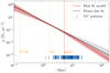 |
Fig. 9. Total mass density of NGC 3115 from the fiducial model. The red solid line with the associated shaded region shows the median, and the 16th and 84th percentiles of the total mass density profile. The red dashed line shows the median scale radius of the total mass density profile. The black solid line and grey shaded regions show the resulting single power-law fit in the region 0.1 < r/Re < 4 and the 1σ uncertainties, as explained in Sect. 5.4. The orange vertical lines show the stellar effective radius and the blue lines indicate the positions of the tracers for reference. |
Depending on the radial region over which we fit the single power-law profile, the resulting power-law slope will vary, as also shown in B18. When considering a larger radial extent, the power-law fit becomes more sensitive to the transition from the inner slope α to the outer slope, fixed to −3. While the profiles agree within the 1σ uncertainty, it is clear that using the single power-law profile will result in a higher density and higher enclosed mass in the outer regions of the galaxy.
6. Comparison with literature
In this section we compare the results from this work with the literature measurements obtained with different dynamical modelling methods and kinematic tracers. We focus on the comparison of the enclosed mass and the slope of the total mass profile. We discuss the results for all 19 galaxies we modelled, but focus on the sample of 12 galaxies with robust measurements determined in Sect. 5.3.
We compare our results with three different studies that systematically investigated the total mass profile of a large subset of SLUGGS galaxies: A16, P17, and B18. Their overlapping science goals, but different kinematic tracers or methodologies, make them uniquely suitable for comparison with our work. A16 determined the enclosed mass with GCs from the SLUGGS survey. They used TME, which assumes spherically symmetric tracer and mass distributions. The inner slope γtot was studied by P17 and B18 with stellar kinematics and axisymmetric JAM. The former used stellar kinematics from the Atlas3D survey (Cappellari et al. 2011) which extends out to 1 Re, and the latter combined the central Atlas3D kinematics with extended stellar kinematics from the SLUGGS survey out to 4 Re. The summary of the literature studies is presented in Table 7.
Properties of the different dynamical studies from the literature in comparison with this work.
6.1. Enclosed mass
We computed the enclosed mass at different radii from model B, as discussed in Sect. 5, and compared it to the literature results from A16. The study modelled 18 of the 19 galaxies presented in this work, and they used GCs with TME. It assumes that both mass density and the tracer density profile are spherically symmetric with a power-law distribution. The slopes are not free parameters in their modelling. Instead, for the GC tracer density slope the authors used literature studies to build an observed correlation between the stellar mass of the host galaxy and the power-law slope of the GCS. To obtain the slope of the total mass density the study uses simulated ETGs and observations to determine the correlation between the logarithmic slope and stellar mass of the galaxy. In their modelling they find that the steeper the slope of either profile, the higher the recovered mass, and thus their treatment of the tracer density profile could result in biased measurements.
Figure 10 shows the enclosed mass within 5 Re as computed from the fiducial set-up described in Sect. 5 on the x-axis, and the values from A16 on the y-axis. We use the A16 masses corrected for flattening, rotation, and presence of kinematic substructures. The dashed line shows the 1–1 line as a guide. The solid black points show galaxies with robust measurements, and we show the galaxies with strong rotation signatures as triangles. These galaxies show no systematic difference in the enclosed mass compared with the galaxies that do not show a strong rotation signature. The greatest outlier is NGC 4564 with a mass measurement that is more than 1σ lower than the literature value. NGC 4365 shows a value that is more than 1σ higher than the total mass.
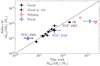 |
Fig. 10. Comparison between the enclosed mass within 5 Re measured using GC kinematics presented in this work and in A16. The measurements on the x-axis were obtained with axisymmetric Jeans models assuming a total mass density profile described by Eq. (6) and on the y-axis the literature study used spherical TME with power-law total mass density distribution. The colours and shapes of the points correspond to those used in other figures. The dashed line is a 1–1 line for comparison and not a fit to the data. We find consistent enclosed mass for galaxies with robust measurements, with the exception of NGC 4564 and NGC 4365, highlighted in the figure, which show more than 1σ lower and higher values, respectively. |
The open red diamonds and blue squares indicate the galaxies with strong subpopulations or other complications in the dynamical modelling. These galaxies deviate most from the 1–1 relation. Blue points indicate three galaxies: NGC 4374, NGC 4526, and NGC 7457. A16 found that NGC 4526 and NGC 7457 have a very large number of GCs in kinematic substructures, 25 out of 107 measured GCs and 6 out of 21, respectively. We did not remove these kinematic substructures, and in the dynamical modelling framework used in this work, the substructures bias the measurements. NGC 4374 is one of the most massive galaxies in the sample, but it has only 41 observed GCs. A16 do not find strong corrections due to rotation, flattening, or kinematic substructures for this galaxy. They compare their measurement with the literature value and find a range of enclosed mass values, suggesting that this galaxy requires great care when inferring its total mass. For our measurement, we conclude that the small number of kinematic tracers is the main driver of the difference with the literature values, but a full investigation is beyond the scope of this work. NGC 4526 shows peculiar kinematics, but has twice the number of GCs than the other two galaxies. With 107 GCs Jeans modelling can reasonably constrain the enclosed mass, but the inner slope is a factor of 2 shallower than the literature studies. Owing to their complex kinematic properties and observational caveats, the measurements of these three galaxies are not robust.
6.2. The power-law slope of the total mass profile
To compare the single power-law profiles with the literature we chose B18 (their model I) and P17 (their model 1). These studies used integrated stellar kinematics in different radial ranges. P17 used central kinematics out to 0.9 Re and B18 extended the measurements to 4 Re. They both used JAM modelling with a cylindrically aligned velocity ellipsoid and the same total mass density profile to which they fit a single power-law slope. The spatial extent of their data does not allow rs to be constrained, so they fix it to 20 kpc. B18 explored how their constraints on the γtot change when rs is left to vary freely. They claim that in this case, the measurements agree within the 1σ uncertainties. Their similar methodology makes these studies ideal for comparison. We find that our results agree within 1σ for the robust sample of galaxies; however, our measurements have a larger spread. We postulate that this could be a consequence of a more flexible modelling approach and fewer data points used to constrain the model.
The comparison of individual galaxies between this work on the x-axis and the literature on the y-axis is shown in Fig. 11. The top panel shows the comparison with P17 for the logarithmic slope within 1 Re and the bottom panel shows the comparison with B18 within 4 Re. The symbols correspond to those in Fig. 6. The black points are the galaxies with robust measurements, and within 1σ uncertainties they agree with the literature values. NGC 1023 is more than 1σ from the dashed 1–1 line and is highlighted in the figure.
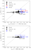 |
Fig. 11. Comparison of the logarithmic slope of the total mass density slope presented in this work on the x-axis and the literature study on the y-axis. The top panel shows the comparison with P17 (model 1) and bottom B18 (model I); the dashed grey line is a 1-to-1 line. The colours and symbols match those in Fig. 6; the solid symbols show robust measurements and the open symbols galaxies excluded from the final analysis. The error bars correspond to the 16th and 84th percentiles, as in Table 6. In both analyses JAM with integrated stellar kinematics was used; this work uses GC kinematics, while the literature studies used stellar kinematics. Within the uncertainties, the measurements of the robust sample agree with the literature values. |
Similarly to the enclosed mass, discussed in Fig. 6, the blue open squares and red open diamonds are systematically lower compared with the literature values. We highlight galaxy NGC 4526, which shows enclosed mass measurements consistent with the literature values in Fig. 10, but the inner slope is more than 1σ shallower than both literature studies. This justifies the exclusion of this galaxy from our robust sample and further supports our initial assignment of kinematic flags.
6.3. Mean value of the inner slope and the intrinsic scatter
After determining the samples with robust measurements we investigate the mean value of the inner slope. We consider both the logarithmic power-law values γtot in different radial ranges and the intrinsic inner slope α. The mean values with respective uncertainties are presented in Table 8 together with a summary of literature results. The first two rows summarise our results followed by the literature values determined using different methodologies and tracers. The first row summarises the results only for galaxies without strong rotation signatures and the second row includes the galaxies with strong rotation signatures of the GCS. The third column shows the mean values and 1σ error for the intrinsic inner total mass density slope α. The fourth column is the mean value of the single power-law fit within 1 Re, for comparison with P17, who determined the inner slope of ⟨γtot⟩1 = −2.193 ± 0.016. The last column shows the mean value for the power-law slope within 0.1–4 Re, comparable with γtot = −2.24 ± 0.05 found by B18.
Mean values of the inner slope and the observed root mean square (rms) scatter for the robust sample of galaxies from this work and the literature studies.
Including only the measured slopes of galaxies flagged as Good results in a slightly shallower slope than when galaxies with strong rotational signatures are included. When investigating the effect of rotation and velocity anisotropy we did not find evidence linking rotation to a steeper profile, and we conclude that our kinematic classification is not linked to the measured values. Our measurements are in broad agreement with these literature studies. Auger et al. (2010) finds slightly shallower slopes, which could be a result of the systematically more massive galaxies that were probed in this study with gravitational lensing. P17 and Yıldırım et al. (2017) use central stellar kinematics, B18 and Cappellari et al. (2015) used extended stellar kinematics, and Serra et al. (2016) combined the central stellar kinematics with extended gas measurements; they all agree within 1σ uncertainties.
The literature studies disagree on the value of the σγtot; Cappellari et al. (2015) and Serra et al. (2016) prefer even smaller intrinsic scatter than Auger et al. (2010) and Serra et al. (2016). This low intrinsic spread has been linked with the universality of the inner total mass slope over several magnitudes in stellar mass. With the novel measurements presented in this work, we attempted to constrain the intrinsic spread of the inner slope σα (e.g., Kirby et al. 2011, Eq. (8)). We find that the measurement uncertainties δα are such that the intrinsic spread cannot be recovered. This is mainly driven by the low average number of GCs per galaxy, which is strongly correlated with the resulting measurement uncertainty, as seen in the left panel of Fig. 12. The figure shows how the δα for each galaxy is correlated with the number of kinematic tracers in the left panel and the median RV error for GCs in the right panel. The measurement uncertainty is strongly correlated with the number of kinematic tracers, while up to the median RV error of 14 km s−1 the δα is not correlated with the velocity errors.
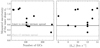 |
Fig. 12. Correlation between the measurement uncertainty of the inner slope (from model B) with the number of GCs per galaxy (left panel) and the median error of the RV (right panel). The grey dashed line indicates the intrinsic scatter of the inner slope of 0.16, as determined by P17 and Auger et al. (2010). In order to constrain the intrinsic slope to the same level, the black solid line indicates the maximum measurement uncertainty needed when using ∼10 galaxies. |
The dashed grey line indicates the literature value of the σγtot ∼ 0.16 consistently found by Auger et al. (2010) and P17. We investigated what limiting precision of α is needed to constrain the intrinsic scatter at the same level with 12 galaxies by artificially scaling δα. The estimate of that limiting precision is shown as the solid black line indicating that at least 100 kinematic tracers per galaxy are needed for sufficient precision. For galaxies with fewer observed GCs the modelling has to be supplemented by stellar kinematics or other halo tracers, such as planetary nebulae, to provide sufficient constraints on the α to recover the intrinsic scatter. Increasing the number of galaxies has an impact on the recoverability of the σα, but more detailed quantification of the observing guidelines is beyond the scope of this work.
6.4. The relation between the inner slope and stellar mass
Several relations have been reported in the literature linking γtot to different properties of the galaxy. Due to the limited number of galaxies with robust measurements, we focus only on the relation between the stellar mass and inner slope; we present our measurements of the intrinsic inner slope α in Fig. 13. The literature values in light blue from P17 were computed with the central stellar kinematics with median radius probed 0.9 Re. Similarly, the orange points show measurements with gravitational lensing (Auger et al. 2010) with median radius probed 0.5 Re.
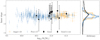 |
Fig. 13. Relation between stellar mass and inner slope (left panel) and distribution of the slopes as determined by this work and literature samples (right panel). The measurements from this work show the intrinsic inner slope α from Eq. (6), those from the literature show the single power-law slope γtot. The black-filled circles and triangles show the galaxies with robust measurements representing the inner mass slope α as measured in this study from the GC kinematics, extending out to ∼8 Re. The symbols are the same as in Fig. 6. Large literature samples focused on the single power-law slope only. They are shown as blue and orange points from Poci et al. (2017) and Auger et al. (2010), respectively. The gravitational lensing from the former study constrained the slope within 0.5 Re, and the latter used stellar kinematics within ∼0.9 Re. The arbitrary scaled distribution of the measurements in the right panel shows the distribution of the slopes with colours corresponding to those in the left panel. |
We do not observe a statistically significant trend of α with the stellar mass. A similar trend is reported by B18 and has also been found in the Magneticum simulations4 (Remus et al. 2017). Tortora et al. (2014) used spherical isotropic Jeans equations to carry out dynamical modelling of SPIDER galaxies over a wide mass range and found that γtot becomes progressively shallower with increasing stellar mass. This trend is not observed by our study or by Cappellari et al. (2015).
The large spatial extent to which the discrete dynamical modelling of GCS is sensitive means that we have tracers beyond the scale radius of the total mass profile. Therefore, the SLUGGS GCs are sensitive to the intrinsic inner total mass slope α and we can compare α to the values from the power-law studies of the inner mass slope, but its interpretation is not straightforward.
7. Discussion
Comparing our results with the literature results from A16, P17, and B18, we investigated various properties of the galaxies for potential trends with the environment (field, group, cluster), baryonic content (stellar mass), (vrot/σ)GCS as reported by A16, flattening of the GCSs, and a number of dynamical tracers on Δγtot. We did not identify any parameters correlated with systematic offset for any of the three literature datasets.
7.1. The link between inner slope and galaxy formation
The apparent universality of the γtot ∼ −2 has been linked to the formation history of the ETGs. Remus et al. (2013) found in merger simulations that dry major mergers redistribute baryonic and dark matter such that the resulting total mass distribution follows a singular isothermal sphere. This configuration is very stable and only the accretion of large amounts of gas can modify the inner slope. Major mergers were more frequent in the earliest phases of galaxy cluster assembly and Derkenne et al. (2021, 2023) recently studied the redshift evolution of γtot finding shallower profiles in cluster galaxies compared to those in intermediate density environments at z ∼ 0.3. The trend persists to z = 0 and galaxies in intermediate density environments, which experience fewer major mergers, show negligible evolution of γtot in the past 3–4 Gyr. Recently, Zhu et al. (2024) showed a strong dependence of the inner slope on the σe and morphological type.
Different galaxy simulations disagree on the values for the inner slope. B18 found that the EAGLE5 simulations (Schaye et al. 2015) produce galaxies with profiles shallower by ∼0.3 − 0.5 than the Magneticum simulations (Remus et al. 2017). Galaxies in the latter simulation additionally show anticorrelation between the stellar mass and the inner slope γtot that is not observed in real galaxies. Moreover, Remus et al. (2017) studied the correlations between the galaxy properties and γtot for three different simulations that vary in whether they incorporate active galactic nuclei (AGN) and star-formation feedback. They find that the AGN feedback in their simulations acts to erase the correlation between the slope and stellar mass of the simulated ETGs. When comparing the results for galaxies from the Magneticum simulation with those from the Oser simulations (Oser et al. 2012) that do not include AGN feedback, they find large discrepancies and systematically steeper values of γtot for Oser simulated ETGs. The study also finds evidence that the slope in simulated galaxies is steeper at higher redshift and that there is a strong anti-correlation between the central stellar surface brightness and γtot.
Literature investigations have repeatedly found a narrow intrinsic spread in γtot (with  ) for ETGs (P17, Auger et al. 2010). Two studies with extended potential tracers found an intrinsic spread of 0.11 for ETGs using stellar kinematics out to 4 Re (Cappellari et al. 2015) and coupling central stellar kinematics with HI circular velocity out to 6 Re (Serra et al. 2016). Studies have found that this bulge–halo conspiracy requires a non-universal stellar initial-mass function and feedback mechanisms to counteract dark matter contraction resulting from dark matter cooling (e.g., Dutton & Treu 2014). However, observations have primarily relied on gravitational lensing or on dynamical modelling based on IFU6. Both provide information well within 1 Re, where the dark matter fraction is on average < 15%. While Auger et al. (2010) used a single power-law slope for the total mass density, P17 had a more realistic double power-law profile with a fixed transition radius. B18 used extended stellar kinematics out to 4 Re. However, the spatial extent of the tracers was not sufficient to freely vary the scale radius of the total mass profile.
Recently, Derkenne et al. (2023) showed that fixing the scale radius has a systematic impact on the recovered slope α. We have also shown that the radial region where the inner slope γtot is fit will impact the recovered value of the parameter, as seen in Table 8, a trend commented on also by B18. With discrete dynamical modelling of the GCs, we have shown in this work that it is possible to recover the intrinsic inner slope of the total mass profile, relaxing the assumption on the scale radius. This opens an avenue for dynamical studies of a larger number of galaxies to probe the intrinsic slope α and better understand the interplay between the baryonic and dark matter physics in the process of galaxy formation.
In this work, we agree with the literature studies and find the mean inner slope γtot is steeper than isothermal, but the exact value of the profile is strongly dependent on the radial range where the profile is fit. Additionally, because of our flexible modelling approach and the large spatial extent of our tracers, our results are sensitive to the intrinsic inner slope of the double power-law profile α. As can be seen in Fig. 9, the projected positions of the GCs in NGC 3115 can also be found around the best-fit scale radius of the total mass profile, meaning that there is enough power in the data to constrain the intrinsic inner slope.
7.2. Limitations of our modelling approach
Discrete dynamical modelling is very flexible, yet great care is needed to understand the intrinsic and observational properties of the GCs. Kinematically cold substructures or biased sampling of the underlying velocity field can result in the biased inference of the modelled parameters, an effect that is strongly dependent on the number of the kinematic tracers.
7.2.1. Effect of subpopulations
A subset of galaxies shows the presence of strong subpopulations that are not relaxed or trace the group or cluster potential instead of the galaxy potential. These galaxies were identified by the rising or constant velocity dispersion out to 7 Re from the centre without a strong presence of rotation. NGC 1407, NGC 4486 (M 87), and NGC 5846 are all the central galaxies of their group. and NGC 4486 is the second brightest galaxy of the Virgo cluster. Their GCS have been extensively studied in the literature.
Zhu et al. (2016) and Napolitano et al. (2014) showed how the velocity dispersion of red GCs in NGC 5846 rises in the outskirts of the galaxy. The red and blue GCs also show distinct orbital anisotropies, with blue showing mild radial anisotropy and red tangential anisotropy in the outskirts. Similarly, Pota et al. (2015) found a kinematically distinct red and blue population of GCs in NGC 1407, with the velocity dispersion of blue GCs increasing towards the outskirts. The Strader et al. (2011) comprehensive kinematic and dynamical study of M 87 (NGC 4486) revealed complexity and a strong presence of substructures in the GCS of the galaxy, pointing to active assembly.
To investigate whether the presence of subpopulations is causing the systematic offsets we modelled separately the blue and red populations of GCS in NGC 1407 as a test case. Romanowsky et al. (2009) carried out a kinematic analysis of the red and blue populations using the colour information (g′−i′) = 0.98 to separate the populations. They found that the dispersion profile decreases until R ∼ 20 kpc and then starts to increase. They report low (vrot/σ)GCS in the outer parts and find signs of misaligned rotation signatures between the red and blue populations with hints of tangentially biased orbits in the outer regions. The blue population shows a presence of a cold moving group around R ∼ 40 kpc.
Following the work by Romanowsky et al. (2009) we separated the two populations of GCs based on their colour. We then carried out the same completeness and tracer density analysis as described in Sect. 3 and re-ran the dynamical modelling. We find that the red population, which is more centrally concentrated and shows declining velocity dispersion in the outer parts, results in a steeper inner slope, in agreement with the literature results. The dispersion profile of the blue population stays flat in the entire radial range, and the resulting inner slope is shallower than that obtained for the red GCs. The enclosed mass measurements from the red population are also in excellent agreement with the literature, while the blue populations result in overestimating the mass by several orders of magnitude. We aim to investigate the other two galaxies and present the results for NGC 1407 in a follow-up study.
7.2.2. Peculiar GCS
A subset of galaxies, NGC 4374, NGC 4459, NGC 4526, and NGC 7457, show peculiar trends in their velocity field. All but NGC 4526 have fewer than 40 GCs sparsely populating their halo. NGC 4526 has a peculiar velocity field in the GCS with the central region showing strong rotation and the outer region showing a velocity offset. This particular galaxy has twice the number of GCs compared with the other galaxies flagged as Subpop., and the recovered enclosed mass is consistent with the literature studies by A16, as highlighted in Fig. 10. However, the inner slope is more sensitive to the peculiar features in the observed GC velocity field, resulting in a biased measurement of the inner slope α shown on Fig. 11.
To understand the discrepancy with the literature studies, we explored trends with the galaxy stellar mass, environment, and rotation parameter as reported by A16, the Sérsic index, and the number of tracers. We found the latter has the strongest impact together with a non-uniform spatial distribution of the tracers. These observational effects result in the shallower profile and overestimated mass when using discrete dynamical modelling. Similar to the galaxies discussed in Sect. 7.2.1 we consider that our measurements for galaxies flagged as Subpop. are not robust.
8. Summary and future work
We carried out the discrete dynamical modelling of a large number of GCSs from the SLUGGS survey. A detailed analysis of the tracer density profile and an investigation of the GC velocity field limited the number of galaxies we modelled from 27 to 21, and we present robust measurements for 12 galaxies. These galaxies have a sufficiently large number of kinematic tracers without a strong observational footprint or presence of subpopulations. We used Bayesian inference and a MCMC sampler to efficiently sample the posterior and find the best-fit parameters. We find that informative priors on log ρs and log rs can help break the degeneracy in these parameters.
We explored three different model set-ups (A, B, C) to investigate how the modelling assumptions impact the best-fit parameters. Models A and B assume non-rotating and isotropic GCs and model C explores the impact of velocity anisotropy and rotation on the recovered parameters of the total mass profile. We find that βz and κ have a negligible impact on the enclosed mass and inner slope. We identify model B as the fiducial model and find the logarithmic inner slope of the 12 galaxies with robust measurements is ⟨γtot⟩= − 2.22 ± 0.14 in the range 0.1–4 Re. These values agree within the uncertainties, but we find that our values are systematically shallower than the literature measurements. This could be a result of our more flexible modelling approach. The large spatial extent of the kinematic tracers in tandem with the discrete modelling approach enables us to constrain the transition radius of the total mass slope and measure the intrinsic inner slope  that is shallower than ⟨γtot⟩.
We find a large rms scatter in the inner slope, which is in part driven by the large measurement uncertainties. We demonstrate that in order to constrain the intrinsic scatter at the level of 0.16 at least 100 kinematic tracers are needed per galaxy.
In Sect. 7.2.1 we have shown that the modelling results of dispersion-dominated systems with CJAM are minimally affected by rotation and anisotropy when the number of tracers is sufficiently large, but providing quantitative guidelines is beyond the scope of this work. When modelling merger remnants and GCS with a strong presence of distinct subpopulations, our results are strongly biased towards overestimating the enclosed mass by several orders of magnitude and a shallower profile.
Simulations and observations both provide strong evidence that the total mass slope cannot be extrapolated with a single power-law profile at a large spatial extent, and new observations will enable both larger photometric and kinematic samples of discrete tracers in the nearby universe. We can use them to characterise the mass distribution on large scales and constrain structure formation models. This work highlights the benefits and caveats of using sparse dynamical tracers in the halos of the galaxies. Combining integrated stellar kinematics in the inner regions with more extended halo tracers can provide stronger constraints on the central mass distribution. Our work can be expanded by including higher Gauss–Hermite moments or assuming an intrinsic 3D Gaussian velocity distribution instead of the 1D projected.
With the upcoming wide-field photometric surveys larger samples of extragalactic GCs will be observed, and this will open an avenue for more studies of these low surface-brightness diffuse halos that contain rich information on the total mass content of galaxies. With the full mass profiles, dark matter content can also be investigated over large galactocentric radii. We would also like to further explore methods to improve the precision of the modelling results and better account for the kinematic substructures.
Acknowledgments
We thank the referee for the helpful comments and suggestions that have improved this manuscript. T.V. thanks Marina Rejkuba, Lucas Valenzuela and Rhea Silvia Remus for their feedback and discussion on the manuscript. This project has received funding from the European Research Council (ERC) under the European Union’s Horizon 2020 research and innovation programme under grant agreement No. 724857 (Consolidator Grant ArcheoDyn). T.V. acknowledges the studentship support from the European Southern Observatory. The computational results presented have been achieved (in part) using the Vienna Scientific Cluster (VSC). This work made use of the following software: NUMPY (Harris et al. 2020), SCIPY (Virtanen et al. 2020), MATPLOTLIB (Hunter 2007), ASTROPY (Astropy Collaboration 2013, 2018, 2022).
References
- Alabi, A. B., Forbes, D. A., Romanowsky, A. J., et al. 2016, MNRAS, 460, 3838 [Google Scholar]
- Astropy Collaboration (Robitaille, T. P., et al.) 2013, A&A, 558, A33 [NASA ADS] [CrossRef] [EDP Sciences] [Google Scholar]
- Astropy Collaboration (Price-Whelan, A. M., et al.) 2018, AJ, 156, 123 [Google Scholar]
- Astropy Collaboration (Price-Whelan, A. M., et al.) 2022, ApJ, 935, 167 [NASA ADS] [CrossRef] [Google Scholar]
- Auger, M. W., Treu, T., Bolton, A. S., et al. 2010, ApJ, 724, 511 [NASA ADS] [CrossRef] [Google Scholar]
- Barnabè, M., Czoske, O., Koopmans, L. V. E., Treu, T., & Bolton, A. S. 2011, MNRAS, 415, 2215 [Google Scholar]
- Bellstedt, S., Forbes, D. A., Romanowsky, A. J., et al. 2018, MNRAS, 476, 4543 [Google Scholar]
- Bílek, M., Samurović, S., & Renaud, F. 2019, A&A, 625, A32 [Google Scholar]
- Brodie, J. P., Romanowsky, A. J., Strader, J., et al. 2014, ApJ, 796, 52 [Google Scholar]
- Cappellari, M. 2002, MNRAS, 333, 400 [NASA ADS] [CrossRef] [Google Scholar]
- Cappellari, M. 2008, MNRAS, 390, 71 [NASA ADS] [CrossRef] [Google Scholar]
- Cappellari, M., Emsellem, E., Krajnović, D., et al. 2011, MNRAS, 413, 813 [Google Scholar]
- Cappellari, M., Scott, N., Alatalo, K., et al. 2013, MNRAS, 432, 1709 [Google Scholar]
- Cappellari, M., Romanowsky, A. J., Brodie, J. P., et al. 2015, ApJ, 804, L21 [NASA ADS] [CrossRef] [Google Scholar]
- Chaturvedi, A., Hilker, M., Cantiello, M., et al. 2022, A&A, 657, A93 [NASA ADS] [CrossRef] [EDP Sciences] [Google Scholar]
- Ciotti, L., & Bertin, G. 1999, A&A, 352, 447 [NASA ADS] [Google Scholar]
- Côté, P., Blakeslee, J. P., Ferrarese, L., et al. 2004, ApJS, 153, 223 [Google Scholar]
- Courteau, S., Cappellari, M., de Jong, R. S., et al. 2014, Rev. Mod. Phys., 86, 47 [Google Scholar]
- De Lucia, G., & Blaizot, J. 2007, MNRAS, 375, 2 [Google Scholar]
- Derkenne, C., McDermid, R. M., Poci, A., et al. 2021, MNRAS, 506, 3691 [NASA ADS] [CrossRef] [Google Scholar]
- Derkenne, C., McDermid, R. M., Poci, A., et al. 2023, MNRAS, 522, 3602 [NASA ADS] [CrossRef] [Google Scholar]
- Dumont, A., Seth, A. C., Strader, J., et al. 2022, ApJ, 929, 147 [NASA ADS] [CrossRef] [Google Scholar]
- Dutton, A. A., & Treu, T. 2014, MNRAS, 438, 3594 [NASA ADS] [CrossRef] [Google Scholar]
- Emsellem, E., Monnet, G., & Bacon, R. 1994, A&A, 285, 723 [NASA ADS] [Google Scholar]
- Fahrion, K., Lyubenova, M., Hilker, M., et al. 2020, A&A, 637, A26 [NASA ADS] [CrossRef] [EDP Sciences] [Google Scholar]
- Forbes, D. A., Almeida, A., Spitler, L. R., & Pota, V. 2014, MNRAS, 442, 1049 [NASA ADS] [CrossRef] [Google Scholar]
- Forbes, D. A., Alabi, A., Brodie, J. P., et al. 2017, AJ, 153, 114 [Google Scholar]
- Foreman-Mackey, D., Hogg, D. W., Lang, D., & Goodman, J. 2013, PASP, 125, 306 [Google Scholar]
- Goodman, J., & Weare, J. 2010, Commun. Appl. Math. Comput. Sci., 5, 65 [Google Scholar]
- Harris, W. E. 1991, ARA&A, 29, 543 [Google Scholar]
- Harris, W. E., Morningstar, W., Gnedin, O. Y., et al. 2014, ApJ, 797, 128 [NASA ADS] [CrossRef] [Google Scholar]
- Harris, W. E., Ciccone, S. M., Eadie, G. M., et al. 2017, ApJ, 835, 101 [NASA ADS] [CrossRef] [Google Scholar]
- Harris, C. R., Millman, K. J., van der Walt, S. J., et al. 2020, Nature, 585, 357 [NASA ADS] [CrossRef] [Google Scholar]
- Hénault-Brunet, V., Gieles, M., Sollima, A., et al. 2019, MNRAS, 483, 1400 [CrossRef] [Google Scholar]
- Hughes, M. E., Jethwa, P., Hilker, M., et al. 2021, MNRAS, 502, 2828 [NASA ADS] [CrossRef] [Google Scholar]
- Humphrey, P. J. 2009, ApJ, 690, 512 [NASA ADS] [CrossRef] [Google Scholar]
- Hunter, J. D. 2007, Comput. Sci. Eng., 9, 90 [NASA ADS] [CrossRef] [Google Scholar]
- Jeans, J. H. 1922, MNRAS, 82, 122 [NASA ADS] [CrossRef] [Google Scholar]
- Jordán, A., Côté, P., Blakeslee, J. P., et al. 2005, ApJ, 634, 1002 [CrossRef] [Google Scholar]
- Jordán, A., Blakeslee, J. P., Côté, P., et al. 2007a, ApJS, 169, 213 [Google Scholar]
- Jordán, A., McLaughlin, D. E., Côté, P., et al. 2007b, ApJS, 171, 101 [CrossRef] [Google Scholar]
- Jordán, A., Peng, E. W., Blakeslee, J. P., et al. 2009, ApJS, 180, 54 [Google Scholar]
- Kartha, S. S., Forbes, D. A., Spitler, L. R., et al. 2014, MNRAS, 437, 273 [NASA ADS] [CrossRef] [Google Scholar]
- Kartha, S. S., Forbes, D. A., Alabi, A. B., et al. 2016, MNRAS, 458, 105 [NASA ADS] [CrossRef] [Google Scholar]
- Kirby, E. N., Cohen, J. G., Smith, G. H., et al. 2011, ApJ, 727, 79 [NASA ADS] [CrossRef] [Google Scholar]
- Kissler-Patig, M. 1997, A&A, 319, 83 [NASA ADS] [Google Scholar]
- Lynden-Bell, D. 1967, MNRAS, 136, 101 [Google Scholar]
- Napolitano, N. R., Pota, V., Romanowsky, A. J., et al. 2014, MNRAS, 439, 659 [NASA ADS] [CrossRef] [Google Scholar]
- Oliva-Altamirano, P., Brough, S., Jimmy, A., et al. 2015, MNRAS, 449, 3347 [CrossRef] [Google Scholar]
- Oser, L., Naab, T., Ostriker, J. P., & Johansson, P. H. 2012, ApJ, 744, 63 [Google Scholar]
- Poci, A., Cappellari, M., & McDermid, R. M. 2017, MNRAS, 467, 1397 [NASA ADS] [Google Scholar]
- Posti, L., & Fall, S. M. 2021, A&A, 649, A119 [NASA ADS] [CrossRef] [EDP Sciences] [Google Scholar]
- Pota, V., Romanowsky, A. J., Brodie, J. P., et al. 2015, MNRAS, 450, 3345 [Google Scholar]
- Read, J. I., Mamon, G. A., Vasiliev, E., et al. 2021, MNRAS, 501, 978 [Google Scholar]
- Rejkuba, M. 2012, Ap&SS, 341, 195 [Google Scholar]
- Remus, R.-S., Burkert, A., Dolag, K., et al. 2013, ApJ, 766, 71 [NASA ADS] [CrossRef] [Google Scholar]
- Remus, R.-S., Dolag, K., Naab, T., et al. 2017, MNRAS, 464, 3742 [Google Scholar]
- Romanowsky, A. J., Strader, J., Spitler, L. R., et al. 2009, AJ, 137, 4956 [NASA ADS] [CrossRef] [Google Scholar]
- Rubin, V. C., Ford, W., & Kent, J. 1970, ApJ, 159, 379 [NASA ADS] [CrossRef] [Google Scholar]
- Sarzi, M., Iodice, E., Coccato, L., et al. 2018, A&A, 616, A121 [NASA ADS] [CrossRef] [EDP Sciences] [Google Scholar]
- Schaye, J., Crain, R. A., Bower, R. G., et al. 2015, MNRAS, 446, 521 [Google Scholar]
- Serra, P., Oosterloo, T., Cappellari, M., den Heijer, M., & Józsa, G. I. G. 2016, MNRAS, 460, 1382 [NASA ADS] [CrossRef] [Google Scholar]
- Sonnenfeld, A., Treu, T., Gavazzi, R., et al. 2013, ApJ, 777, 98 [Google Scholar]
- Strader, J., Romanowsky, A. J., Brodie, J. P., et al. 2011, ApJS, 197, 33 [NASA ADS] [CrossRef] [Google Scholar]
- Tortora, C., La Barbera, F., Napolitano, N. R., et al. 2014, MNRAS, 445, 115 [NASA ADS] [CrossRef] [Google Scholar]
- van de Ven, G., van den Bosch, R. C. E., Verolme, E. K., & de Zeeuw, P. T. 2006, A&A, 445, 513 [NASA ADS] [CrossRef] [EDP Sciences] [Google Scholar]
- Villegas, D., Jordán, A., Peng, E. W., et al. 2010, ApJ, 717, 603 [Google Scholar]
- Virtanen, P., Gommers, R., Oliphant, T. E., et al. 2020, Nat. Methods, 17, 261 [Google Scholar]
- Watkins, L. L., Evans, N. W., & An, J. H. 2010, MNRAS, 406, 264 [Google Scholar]
- Watkins, L. L., van de Ven, G., den Brok, M., & van den Bosch, R. C. E. 2013, MNRAS, 436, 2598 [Google Scholar]
- White, S. D. M., & Rees, M. J. 1978, MNRAS, 183, 341 [Google Scholar]
- Yıldırım, A., van den Bosch, R. C. E., van de Ven, G., et al. 2017, MNRAS, 468, 4216 [Google Scholar]
- Zepf, S. E., Geisler, D., & Ashman, K. M. 1994, ApJ, 435, L117 [NASA ADS] [CrossRef] [Google Scholar]
- Zhu, L., Romanowsky, A. J., van de Ven, G., et al. 2016, MNRAS, 462, 4001 [Google Scholar]
- Zhu, K., Lu, S., Cappellari, M., et al. 2024, MNRAS, 527, 706 [Google Scholar]
All Tables
Basic information for the 21 galaxies from the SLUGGS survey modelled in this work.
Results from the analysis of the tracer density profile fitting and completeness.
Single power-law slope of the total mass density profile in different radial ranges; the kinematic flags are listed in the last column.
Properties of the different dynamical studies from the literature in comparison with this work.
Mean values of the inner slope and the observed root mean square (rms) scatter for the robust sample of galaxies from this work and the literature studies.
All Figures
|
Fig. 1. Position of the GCs from the SLUGGS survey are shown as blue and orange points. The orange points are selected based on their position as more likely belonging to NGC 5845, and the blue points show the NGC 5846 GCs used in this work. The positions and systemic velocities shown as coloured crosses for the four galaxies are from Simbad (https://simbad.unistra.fr/simbad/). |
| In the text | |
|
Fig. 2. Example of spatial and magnitude distribution of the kinematic tracers. Both were used to determine an observationally unbiased sample of GCs to construct the tracer density profile for each galaxy. The left panel shows the spatial distribution of the GCs in NGC 3377 centred at the coordinates of the host galaxy and aligned with the photometric position angle. The GCs are colour-coded by their velocity corrected for the systemic velocity of the galaxy. The kinematic tracers extend beyond 9 Re. The solid grey line in the right panel shows the GCLF of NGC 3377. The dashed black curve shows the arbitrarily scaled theoretical GCLF; the turn-over magnitude is indicated with a vertical solid black line. The vertical dotted line shows the magnitude completeness of the sample, determined as described in the text. |
| In the text | |
|
Fig. 3. Sérsic fit to the binned tracer density profile for NGC 3377 in elliptical radius. The binned profile is represented by black points. The best-fit model is shown with the solid red line with 1 and 3σ uncertainty regions indicated with dark and light grey shaded regions, respectively. |
| In the text | |
|
Fig. 4. Posterior of model B for NGC 3377. The median and the 1σ percentiles are shown as dashed lines on each of the marginalised posteriors and the corresponding values are given at the top. |
| In the text | |
|
Fig. 5. Comparison between informative priors for log10ρs and log10rs as coloured lines for model A and model B and the posteriors for each of the 21 modelled galaxies as grey lines. In fiducial model B the widths of the posteriors are narrower than those of the priors, which indicates that the data is driving the posterior, not the prior. |
| In the text | |
|
Fig. 6. Effect of informative priors on enclosed mass within 5 Re. The black dots and triangles show galaxies flagged as Good and Good w. rot., respectively, as defined in Sect. 2.2. The measurements for these galaxies are robust. The open red diamonds and blue squares are galaxies flagged as Subpop. and Pecul., respectively, and for which the measurements are not robust. The dashed line is a 1–1 line for reference. |
| In the text | |
|
Fig. 7. Comparison between the best-fit results from models B and C and the data for NGC 3115 along the semi-major axis of the galaxy. The top panel shows the mean velocity and the bottom the velocity dispersion. The blue triangles and squares show the mean velocity and velocity dispersion of the GCs, respectively. The black dashed line shows the velocity dispersion computed with the best-fit parameters of model B. The solid red line shows the same for model C. The vertical grey lines show multiples of the stellar effective radius for comparison. |
| In the text | |
|
Fig. 8. Best-fit velocity anisotropy and rotation from model C. The symbols match those in Fig. 6; the black points are the galaxies with robust measurements and the open symbols those without. The top panel shows the velocity anisotropy for each galaxy and the bottom panel shows the rotation parameter κ. The error bars highlight the 16th and 84th percentile uncertainty on the measurement. The dashed grey line shows the isotropic βz = 0 and non-rotating κ = 0 values for reference. |
| In the text | |
|
Fig. 9. Total mass density of NGC 3115 from the fiducial model. The red solid line with the associated shaded region shows the median, and the 16th and 84th percentiles of the total mass density profile. The red dashed line shows the median scale radius of the total mass density profile. The black solid line and grey shaded regions show the resulting single power-law fit in the region 0.1 < r/Re < 4 and the 1σ uncertainties, as explained in Sect. 5.4. The orange vertical lines show the stellar effective radius and the blue lines indicate the positions of the tracers for reference. |
| In the text | |
|
Fig. 10. Comparison between the enclosed mass within 5 Re measured using GC kinematics presented in this work and in A16. The measurements on the x-axis were obtained with axisymmetric Jeans models assuming a total mass density profile described by Eq. (6) and on the y-axis the literature study used spherical TME with power-law total mass density distribution. The colours and shapes of the points correspond to those used in other figures. The dashed line is a 1–1 line for comparison and not a fit to the data. We find consistent enclosed mass for galaxies with robust measurements, with the exception of NGC 4564 and NGC 4365, highlighted in the figure, which show more than 1σ lower and higher values, respectively. |
| In the text | |
|
Fig. 11. Comparison of the logarithmic slope of the total mass density slope presented in this work on the x-axis and the literature study on the y-axis. The top panel shows the comparison with P17 (model 1) and bottom B18 (model I); the dashed grey line is a 1-to-1 line. The colours and symbols match those in Fig. 6; the solid symbols show robust measurements and the open symbols galaxies excluded from the final analysis. The error bars correspond to the 16th and 84th percentiles, as in Table 6. In both analyses JAM with integrated stellar kinematics was used; this work uses GC kinematics, while the literature studies used stellar kinematics. Within the uncertainties, the measurements of the robust sample agree with the literature values. |
| In the text | |
|
Fig. 12. Correlation between the measurement uncertainty of the inner slope (from model B) with the number of GCs per galaxy (left panel) and the median error of the RV (right panel). The grey dashed line indicates the intrinsic scatter of the inner slope of 0.16, as determined by P17 and Auger et al. (2010). In order to constrain the intrinsic slope to the same level, the black solid line indicates the maximum measurement uncertainty needed when using ∼10 galaxies. |
| In the text | |
|
Fig. 13. Relation between stellar mass and inner slope (left panel) and distribution of the slopes as determined by this work and literature samples (right panel). The measurements from this work show the intrinsic inner slope α from Eq. (6), those from the literature show the single power-law slope γtot. The black-filled circles and triangles show the galaxies with robust measurements representing the inner mass slope α as measured in this study from the GC kinematics, extending out to ∼8 Re. The symbols are the same as in Fig. 6. Large literature samples focused on the single power-law slope only. They are shown as blue and orange points from Poci et al. (2017) and Auger et al. (2010), respectively. The gravitational lensing from the former study constrained the slope within 0.5 Re, and the latter used stellar kinematics within ∼0.9 Re. The arbitrary scaled distribution of the measurements in the right panel shows the distribution of the slopes with colours corresponding to those in the left panel. |
| In the text | |
Current usage metrics show cumulative count of Article Views (full-text article views including HTML views, PDF and ePub downloads, according to the available data) and Abstracts Views on Vision4Press platform.
Data correspond to usage on the plateform after 2015. The current usage metrics is available 48-96 hours after online publication and is updated daily on week days.
Initial download of the metrics may take a while.